Abstract
We illustrate how structural equation models (SEMs) can be used to assess the reliability and generalizability of composite and subscale scores, proportions of multiple sources of measurement error, and subscale added value within multivariate designs using data from a popular inventory measuring hierarchically structured personality traits. We compare these techniques between standard SEMs representing congeneric relations between indicators and underlying factors versus SEM-based generalizability theory (GT) designs with simplified essential tau-equivalent constraints. Results strongly emphasized the importance of accounting for multiple sources of measurement error in both contexts and revealed that, in most but not all instances, congeneric designs yielded higher score accuracy, lower proportions of measurement error, greater average subscale score viability, stronger model fits, and differing magnitudes of disattenuated subscale intercorrelations. Extending the congeneric analyses to the item level further highlighted consistent weaknesses in the psychometric properties of negatively versus positively keyed items. Collectively, these findings demonstrate the practical value and advantages of applying GT-based principles to congeneric SEMs that are much more commonly encountered in the research literature and more directly linked to the specific measures being analyzed. We also provide prophecy formulas to estimate reliability and generalizability coefficients, proportions of individual sources of measurement error, and subscale added-value indices for changes made to measurement procedures and offer guidelines and examples for running all illustrated analyses using the lavaan (Version 0.6-17) and semTools (Version 0.5-6) packages in R. The methods described for the analyzed designs are applicable to any objectively or subjectively scored assessments for which both composite and subcomponent scores are reported.
Keywords:
structural equation modeling; generalizability theory; multivariate analysis; factor analysis; reliability; subscale added value; disattenuated correlation coefficients; Big Five Inventory; R programming; confidence intervals MSC:
62P15
1. Introduction
Generalizability theory (G-theory; [1,2,3,4,5,6,7,8,9,10,11,12,13,14,15]) combines concepts from classical test theory and analysis of variance (ANOVA) procedures to form a comprehensive framework for understanding how scores from assessment measures are affected by multiple sources of measurement error and subsequently using that information to evaluate and improve such measures. When objectively scored self-report questionnaires or multiple-choice tests are administered in which all scorers would obtain the same results, persons × items × occasions (pio) designs can be used to reduce confounding of universe scores with hidden sources of measurement error and separate such error into three independent components that reflect inter-person differences in item scores (specific-factor error/method effects), occasion scores (transient error/state effects), and other unrelated error (random-response error/within-occasion “noise” effects; see, e.g., [13,14,15]). Such designs further allow for assessment of results that would be obtained from simpler designs involving just items or just occasions as measurement facets (i.e., persons × items (pi) and/or persons × occasions (po) designs) and for estimating key indices (generalizability coefficients, proportions of measurement error, etc.) when changing numbers of facet conditions (i.e., items and/or occasions here).
Although introduced long ago [4], multivariate G-theory designs have been applied far less often across disciplines than have their univariate counterparts even though multivariate designs provide more appropriate indices of score accuracy for composites, while simultaneously yielding results identical to univariate analyses for each individual subscale. Multivariate G-theory designs can also produce correlations between subscale scores corrected for all relevant sources of measurement error to provide additional evidence of concurrent and construct validity for subscale scores (see, e.g., [10,16,17]).
Historically, G-theory has been applied more often to subjectively than to objectively scored measures, with recent examples spanning disciplines that include educational psychology and measurement [18,19,20,21,22], medical education [23,24,25,26,27,28,29,30,31], school psychology [32,33,34,35,36,37], classroom assessment [38,39], second language education and linguistics [40,41,42], thinking skills and creativity [43], music performance [44], athletic training [45], job performance [46], and many other areas. This makes sense because raters typically change over situations, and focal indices of reliability in G-theory (e.g., generalizability or G coefficients) represent the extent to which results can be generalized to broader domains of all possible raters. However, the notion that items and occasions for objectively scored measures are randomly sampled or exchangeable with those from such broader domains is certainly debatable (see, e.g., [47]). Moreover, the broader focus of G-theory-based indices of score accuracy is at odds with conventional reliability coefficients for objectively scored measures (alpha, omega, test–retest) that relate directly to the specific measures administered and limit inferences to items and occasions that share the same characteristics as those being analyzed.
To increase the flexibility of G-theory techniques, structural equation models (SEMs) can be used to derive indices applicable either to the specific conditions considered in a study or to the broader domains from which items and occasions are sampled [15,48,49,50]. This is typically accomplished by allowing unstandardized factor loadings to vary in congeneric (CON) models but setting them equal in traditional G-theory models to render essential tau-equivalent (ETE) relationships. When applying both frames of reference to univariate [15,48,50] and bifactor model [49] designs, Vispoel and colleagues found that CON models yielded higher reliability coefficients and better fits to the data due primarily to reductions in inter-person item (i.e., specific-factor error/method) effects. However, these techniques have yet to be comprehensively applied to multivariate designs that produce more suitable indices of score accuracy for composite scores by taking subscale representation and interrelationships into account.
Specifically, our goals in this article are to illustrate how multivariate SEMs can be used to (a) evaluate how well models with ETE and CON constraints fit the data at hand, (b) estimate relevant indices of score accuracy and proportions of measurement error within each analyzed design, (c) extend partitioning of observed score variance to the item level within appropriate designs, (d) produce correlation coefficients between subscale scores corrected for all pertinent sources of measurement error, (e) apply techniques to assess value gained when reporting subscales in addition to composite scores, and (f) derive indices of score accuracy and added value when changes are made to numbers of items or occasions within a design and/or when those designs are simplified to include just items or just occasions.
2. Background
2.1. Partitioning of Observed Score Variance within Common Multivariate Designs
To illustrate applications of ETE and CON relationships within multivariate analyses, we will use data for selected scales from the recently revised and expanded form of the Big Five Inventory (BFI-2; [51]) that was completed by a large sample of college students on two occasions, a week apart. Our illustrations represent the global personality domain Extraversion and its nested subdomain facets Assertiveness, Energy Level, and Sociability using a persons × items × occasions (p × i × o) multivariate design. Within this design, subscales are considered fixed because inferences do not extend beyond the constructs measured by those subscales. In more technical terms (see, e.g., [10]), this multivariate design would be formally labeled as a design, with the closed circles indicating that persons and occasions are crossed with subscales (i.e., all persons complete all subscales on all occasions) and the open circle indicating that items are nested within subscales (i.e., different items appear in each subscale). At both subscale and composite score levels for objectively scored self-report measures, the design allows for separation of explained (i.e., trait, person, universe score, or true score) variance () and three independent sources of measurement error variance that are often labeled as specific-factor (), transient (), and random-response error variance (; see e.g., [52,53,54], also see [55]). These sources of measurement error, in turn, limit the extent to which results can be generalized to the targeted domain(s) of interest.
The subscript p in the variance terms for the three components of measurement error described above indicates that such errors are person specific. Specific-factor error represents enduring effects such as understandings of words within items and response options that are unrelated to the targeted construct(s) being measured. Transient error represents effects pervasive within an occasion of assessment but not across occasions that result from respondent dispositions, mindsets, and physiological conditions; their reactions to administration and environmental factors; and other temporary entities that affect overall behavior within an occasion. Random-response error corresponds to fleeting within-occasion “noise” effects that follow no systematic pattern (distractions, momentary lapses in attention, fluctuations in moods, changes in motivation, etc.). In designs illustrated within this article, random-response error also would include any remaining residual error not captured by other components in the design, as reflected in the inclusion of “,e” in the subscript for the random-response error variance component (). In frameworks such as latent state-trait theory [15,56,57], person, specific-factor error, transient error, and random-response error are respectively labeled as trait, method, state, and error effects, with method and/or state effects treated as explained rather than measurement error variance when computing several types of reliability indices reported within that framework (e.g., reliability, common reliability, total consistency; see [15] for an in-depth discussion of relationships between G-theory and latent state-trait theory and parallel labels typically used to describe various indices of score accuracy).
2.2. Multivariate ETE and CON SEMs
In Figure 1, we depict a SEM to represent a multivariate design for the three subdomain-facet subscales (Assertiveness, Energy Level, and Sociability) within the Extraversion personality domain from the BFI-2 that can be adjusted to represent either ETE or CON relationships. The SEM has a separate factor to represent person/trait scores for each subscale, and these factors are allowed to covary/correlate with each other. For each subscale, there are separate factors for each item linked to all occasions, separate factors for each occasion linked to all items within that occasion, and uniquenesses for each item within each occasion. Because all subscales are administered during the same occasion, occasion factors among subscales also are allowed to covary/correlate within, but to the same degree, across occasions. Together, the modeling represents a separate univariate, persons × items × occasions design for each subscale, which are linked together by covariances among the subscale person and occasion factors to create the overall multivariate design. Relationships between subscale scores within the designs are instrumental in deriving appropriate estimates of score accuracy for composites that will generally exceed those in magnitude than when derived for the same composites ignoring subscale representation and interrelationships [see, e.g., [4,58,59]].
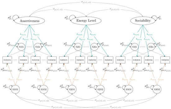
Figure 1.
Structural equation model for S-ETE and CON G-theory designs for Extraversion domain subscales. Note. p = Person; S = Subscale; I = Item; O = Occasion; = person, universe score, or trait variance; = specific-factor error variance; = transient error variance; and = random-response error variance. Symbols linking subscales at the top of the model and linking occasions at the bottom of the model represent covariances. Lines shown in blue and brown respectively represent loadings for items and occasions. For simplified essential tau-equivalent (S-ETE) designs, and are set equal to 1, and and are set equal within a subscale but allowed to vary across subscales. For congeneric (CON) designs, and are set equal to 1, and , β, , and are allowed to differ across items but not across occasions.
To define ETE relationships within the SEM depicted in Figure 1, all factor loadings (λs and βs) are set equal to one, and , , and terms are, respectively, set equal within but not across subscales. Although uniquenesses for each subscale could be allowed to vary within an ETE model, they are set equal here to simplify the calculation of variance components (see, e.g., [16,59]). Consequently, we will call this a simplified essential tau-equivalent (S-ETE) design hereafter. For the corresponding CON design, and terms for each subscale are set equal to one, and , , , and values are allowed to differ within but not across occasions. Once these parameters are estimated, they can be placed in equations shown in Table 1 to derive variance components for persons, specific-factor error, transient error, and random-response error on the item score metric for composite or subscale scores. These variance components, in turn, can be inserted into Equations (1)–(4) to derive proportions of variance due to person/trait, specific-factor error (SFE), transient error (TE), and random-response error (RRE) effects. The proportion of person/trait variance would be equivalent to a generalizability or G coefficient in the context of G-theory. Because item loadings can vary within CON designs, partitioning of explained and measurement error variance also can be extended to the individual item level, as we will demonstrate later in this article.
where SFE = specific-factor error, TE = transient error, and RRE = random-response error.

Table 1.
Formulas for partitioning of variance components for multivariate designs.
2.3. Deriving G Coefficients for More Restricted Universes of Generalization
Once variance components for SFE, TE, and RRE are obtained for a pio univariate or multivariate design, they can be inserted into Equations (5) and (6) to derive G coefficients for pi and po designs. The corresponding multivariate versions of these designs would respectively be labeled as and designs, again because items are nested under subscales and persons and occasions are crossed with subscales. Equations (5) and (6) reveal that TE is treated as part of person/trait variance in the pi design, whereas SFE is treated as part of person/trait variance in the po design. Confounding of effects for persons and TE within pi designs parallels the same confounding of those effects when estimating conventional single occasion reliability coefficients (alpha, omega, split-half). Similarly, confounding of effects for persons and SFE within po designs parallels the same confounding when estimating conventional test–retest coefficients.
where SFE = specific-factor error, TE = transient error, and RRE = random-response error.
2.4. Correcting Subscale Intercorrelation Coefficients for Multiple Sources of Measurement Error
An important advantage of analyzing multivariate designs is that results can be used to correct correlation coefficients between subscale observed scores for multiple sources of measurement error. Such corrections can be interpreted in relation to the classic disattenuation formula shown in Equation (7) first proposed by Spearman ([60]; also see [61]).
where = estimated correlation between true scores for measures and , = observed correlation coefficient between measures and , = reliability coefficient for measure , and = reliability coefficient for measure .
In this formula, the correlation between true scores for measures and is estimated by dividing the correlation between observed scores for the measures by the square root of the product of their reliability coefficients. In G-theory, G coefficients for the measures of interest would be substituted for conventional reliability coefficients, and universe scores would be substituted for true scores (see, e.g., [62,63]). True scores would represent the specific items included in measures and , whereas universe scores based on the same items serve as proxies for all possible items within the domains from which items are sampled. The same relationships would hold if occasions or other measurement facets are included in the design.
2.5. Evaluating Subscale Added Value
A common question addressed when using measures that produce both subscale and composite scores is whether subscale scores provide information or “added value” beyond that provided by composite scores. A useful classical test theory-based method for answering this question originally proposed by Haberman ([64]; also see [65,66,67,68,69]) is to compare proportional reductions in mean squared error (PRMSE) in estimating a subscale’s true scores using observed scores from the subscale versus its associated composite. Vispoel, Lee, Hong, and Chen ([17]; also see [59,70]) noted that Haberman’s procedure also can be readily applied to G-theory designs by substituting universe score for true score estimation. In the present context, these extensions would encompass both S-ETE and CON SEMs.
When interpreting Haberman’s procedure, a subscale would demonstrate added value if its PRMSE exceeds that for its corresponding composite scale. The PRSME for a subscale reduces to its reliability coefficient (either conventional or G-theory-based), whereas the PRSME for the composite scale can be computed using Equation (8).
where = true score, = observed score, = subscale, = composite score, and = composite reliability.
In essence, a PRMSE index represents an estimate of the proportion of true or universe score variance that is accounted for by targeted observed scores (subscale or composite; [67,68]). Once PRMSEs are derived for a subscale and its associated composite scale, they can be placed in Equation (9) to form a value-added ratio (VAR; [69]). Subscale added value is increasingly supported as VARs deviate upwardly from 1.00.
2.6. Estimating Score Accuracy and Subscale Added Value When Changing Measurement Procedures
One of the greatest virtues of G-theory is that it allows for estimation of score accuracy for changes made to a measurement procedure (e.g., including additional items and/or occasions). These techniques can be applied to both the S-ETE and CON multivariate SEMs considered here and further extended to estimation of value-added indices. The main difference between the two approaches again is that inferences for the CON designs would be restricted to items and occasions like those sampled rather than the broader domains from which they are drawn. In Table 2, we present formulas that can be used to estimate score accuracy and value-added indices for changes made to numbers of items and/or occasions for the original and more restricted and designs, and demonstrate their application in later sections.
Table 2.
Prophecy formulas for generalizability/reliability coefficients and value-added ratios.
3. Motivation for and Purpose of the Study
Reliability coefficients routinely reported in research studies (alpha [71], omega [72], also see [73], split-half [61,74], etc.) are limited to single occasions and typically inflated because they do not properly account for all relevant sources of measurement error. This, in turn, can lead to underestimation of relationships between constructs when those reliability coefficients are used to correct for measurement error (see Equation (7)). When reliability coefficients are reported for composite scores in such studies, they often consist of alpha coefficients derived from all item scores ignoring subscale representation and interrelationships, thereby potentially leading to underestimation of composite score reliability in those contexts [4,58,59]). Multivariate G-theory can provide solutions to both problems by producing coefficients of score accuracy that account for all relevant sources of measurement error at both subscale and composite levels and by adjusting for subscale representation and interrelations at the composite level [10,16,17]. Such designs further allow for derivation of correlation coefficients between subscale scores corrected for multiple sources of measurement error and indices for each subscale that reflect their added value beyond the composite.
However, generalizability coefficients in applications of G-theory tend to be conservative in nature because they reflect random equivalence across all possible indicators within the global assessment domain(s) of interest (see, e.g., [1,2,11]). While such indices are often of interest (e.g., when raters repeatedly change across measurements), they are at odds with most conventional reliability coefficients that are catered to the specific conditions (e.g., items) considered for a given assessment procedure. Within multivariate SEMs, measures at hand are represented by CON relationships between indicators and factors, whereas random equivalence across broader domains is represented by corresponding S-ETE relationships.
Our purpose here is to illustrate and contrast both approaches (CON and S-ETE) in relation to model fit, coefficients of score accuracy, partitioning of composite and subscale observed score variance, subscale intercorrelation coefficients, and subscale added-value indices using selected scores from the BFI-2. We further demonstrate how to estimate generalizability/reliability and subscale added-value indices when making changes to the measurement procedures. Within sections to follow, we first describe the participant sample, measures used, and analyses in greater detail; then, present results for comparisons between the S-ETE and CON SEMs; and lastly, illustrate how to use prophecy formulas to estimate generalizability/reliability and value-added indices when increasing numbers of items and/or occasions. Our Supplementary Materials include further instruction and computer code for performing the key analyses.
4. Methods
Participants, Measures, and Procedure
We collected data from 389 college students from a Midwestern Research One institution (71.72% female, 70.95% Caucasian, mean age = 20.38) who completed online versions of the Big Five Inventory (BFI-2; [51]) on two occasions separated by a week. The study was preapproved by the governing Institutional Review Board (ID# 200809738), and all participants provided informed consent before completing the measures. For sake of brevity, we limit results reported here to the Extraversion domain composite and its nested subscale scores Assertiveness, Energy Level, and Sociability, but the same procedures could be applied to the remaining personality domains represented in the BFI-2 or to composite and nested subscale scores for any other assessment procedure. Each BFI-2 composite scale has twelve items, with three nested subscales that each have four items, equally balanced for positive and negative phrasing. Items are answered using a 5-point Likert-style rating scale (1 = Disagree strongly, 2 = Disagree a little, 3 = Neutral, no opinion, 4 = Agree a little, and 5 = Agree strongly).
Evidence supporting the reliability and validity for BFI-2 Extraversion composite and subscale scores reported by Soto and John [51] for college and/or internet samples includes (a) alpha reliability coefficients equaling 0.88 for the composite score and ranging from 0.72 to 0.85 for subscale scores, (b) 8-week test–retest coefficients equaling 0.84 for the composite score and ranging from 0.74 to 0.83 for subscale scores, (c) self-peer agreement correlation coefficients for Extraversion composite and subscales exceeding the same correlation coefficients for other personality domains, (d) correlation coefficients for subscales within the Extraversion domain exceeding those across other personality domains, (e) confirmed patterns of convergent and discriminant validity with scores from other personality and related measures, and (f) adequate model fits for confirmatory correlated factor models for the subscales when controlling for acquiescence bias.
5. Analyses
Preliminary analyses for BFI-2 Extraversion composite and subscale scores included estimation of means, standard deviations, alpha [71] and omega [72] reliability coefficients for each occasion as well as test-retest reliability coefficients across occasions. Main analyses focused on model fit tests, partitioning of observed score variance for the multivariate S-ETE and CON designs in addition to disattenuated correlations and VARs for subscale scores within those designs. We considered model fits for the original designs as adequate when Comparative Fit Index (CFI) and Tucker–Lewis Index (TLI) values equaled or exceeded 0.90 and Root Mean Squared Error of Approximation (RMSEA) values were no higher than 0.08; and as excellent when CFIs and TLIs equaled or exceeded 0.95 and RMSEA values were no higher than 0.06 [75,76,77].
Within each original or restricted design, proportions of observed composite and subscale score variances were derived for universe/factor trait scores and associated sources of measurement error. The same partitioning of explained and measurement error variance was extended to the item level for the CON design to determine which items were most affected by particular sources of error (specific factor, transient, and random response). Disattenuated correlation coefficients between subscale universe or factor trait scores within the S-ETE and CON designs were estimated by dividing the relevant observed score correlation coefficient by the square root of the products of corresponding generalizability/reliability coefficients (see Equation (7)). VARs were derived for each subscale within the original and reduced facet S-ETE and CON designs, with values greater than 1.00 indicative of added value beyond the associated composite. We further demonstrate how formulas from Table 2 can be used to estimate generaliability/reliability coefficients and value-added ratios (VARs) when doubling numbers of items and/or pooling results across two occasions within the , , and multivariate designs. SEMs were analyzed using the lavaan package (Version 0.6-17) in R [78,79] with maximum likelihood (MLM) parameter estimation. Additional code was included to derive disattenuated correlation coefficients and VARs for all subscales and to produce 95% Monte Carlo-based confidence intervals [80] for relevant indices using the semTools package (Version 0.5-6) in R ([81]; see online Supplementary Materials).
6. Results
6.1. Descriptive Statistics and Conventional Reliability Estimates
Table 3 includes means, standard deviations, and conventional reliability estimates for BFI-2 Extraversion composite and subscale scores. Overall, item scale means range from 3.319 to 3.332 (M = 3.326) for composite scores and from 3.187 to 3.562 for subscales (M = 3.326); item scale standard deviations range 0.696 to 0.711 (M = 0.704) for composite scores and from 0.784 to 0.983 (M = 0.861) for subscales; alpha coefficients range from 0.843 to 0.850 (M = 0.847) for composites and from 0.655 to 0.791 (M = 0.731) for subscales; omega coefficients range from 0.848 to 0.855 (M = 0.852) for composites and from 0.685 to 0.793 (M = 0.747) for subscales; and test–retest coefficients equal 0.898 for the composite and range from 0.823 to 0.896 (M = 0.855) for subscales. As would be expected, due to inclusion of more item scores (12 vs. 4), reliability coefficients for composites, on average, exceed those for subscales (0.847 vs. 0.731 for alpha, 0.852 vs. 0.747 for omega, and 0.898. vs. 0.855 for test–retest).
Table 3.
Means, standard deviations, and conventional reliability estimates for BFI-2 Extraversion composite and subscale scores (n = 389).
6.2. Model Fit
CFI, TLI, and RSMEA values for the multivariate designs represented in Figure 1 indicate that the model with CON relationships adequately fits the data (CFI = 0.941, TLI = 0.934, RMSEA = 0.058), but the model with S-ETE relationships does not (CFI = 0.853, TLI = 0.857. RMSEA = 0.085). However, the lack of adequate fit for the S-ETE design does not invalidate its use within G-theory contexts because no assumptions are made in G-theory concerning score dimensionality or other statistical characteristics of item scores [1] (p. 145). Nevertheless, for the data at hand, the less restricted CON model clearly provides a better fit.
6.3. Partitioning of Total Observed Score Variance within the S-ETE and CON Designs
In Table 4, we report estimates of all relevant indices (factor loadings, uniquenesses, variances) needed to derive proportions of universe/factor trait and measurement error variance using formulas shown in Table 1, and report those results for Extraversion composite and subscale scores within the S-ETE and CON designs in Table 5. Consistent with the conventional reliability coefficients previously described, generalizability/reliability coefficients representing multiple sources of measurement error for the designs within Table 5 are uniformly higher for composite scores (0.816 for S-ETE and 0.819 for CON) than for subscale scores (Ms = 0.691 for S-ETE and 0.696 for CON) and higher for the CON design than the S-ETE design for all scales except Sociability. Partitioning of variance for both S-ETE and CON designs underscores the importance of taking all three sources of measurement error into account, with specific-factor, transient, and random-response measurement error, on average, respectively accounting for proportions of observed score variance in the S-ETE/CON designs equaling 0.081/0.080, 0.052/0.050, and 0.050/0.051 at the composite level and 0.164/0.158, 0.040/0.044, and 0.105/0.103 at the subscale level.
Table 4.
Factor loadings, factor variances, residuals, and variance components for BFI-2 Extraversion domain items within the multivariate SEM designs.
Table 5.
Generalizability/reliability coefficients and proportions of measurement error for BFI-2 Extraversion composite and subscale scores within the multivariate SEM designs.
Table 5 also includes proportions of person/trait variance and overall measurement error for composite and subscale scores when measurement facets are restricted to just items ( multivariate designs) or just occasions ( multivariate designs). Due to transient error being treated as part of person/trait variance within the design (see Equation (5)) and specific-factor error being treated as part of person/trait variance within the design (see Equation (6)), generalizability/reliability coefficients in those designs exceed corresponding ones within the designs at both composite and subscale levels in all instances. Additionally, note that reliability coefficients for the restricted CON designs exceed generalizability coefficients for S-ETE designs in most but not all instances.
The 95% confidence intervals for all generalizability/reliability coefficients and nearly all proportions of measurement error in Table 5 fail to capture zero. The only exception is with the confidence interval for the Energy Level subscale’s proportion of transient error within the design that captures zero in the S-ETE design but not in the CON design. As would be expected, proportions of specific-factor and random-response error are noticeably lower for composite than for subscale scores within that design, again likely due to the composite scale having three times as many items. For the same reason, composite score generalizability/reliability coefficients also exceed corresponding subscale score coefficients within the more restricted and designs.
6.4. Item-Level Partitioning of Observed Score Variance within the CON Design
A key advantage of allowing factor loadings to vary across items in the CON design is that partitioning of observed score variance can be extended to the item level. Such information can be extremely useful in instrument development and revision for choosing items that display desired patterns of partitioning for observed score variance. With measures of psychological traits like those considered here, items within the CON design would typically be chosen to maximize explained trait score variance and minimize all relevant sources of measurement error.
To illustrate, we report proportions of trait score and measurement error variance for all items within the Assertiveness, Energy Level, and Sociability subscales in Table 6. Results in the table reveal that the desired pattern of partitioning is realized to a much greater extent with positively than with negatively keyed items. Specifically, in comparison to positively keyed items, negatively keyed items, on average, have noticeably lower proportions of trait score variance (0.224 vs. 0.611), noticeably higher proportions of specific-factor (0.489 vs. 0.170) and random-response (0.278 vs. 0.169) error variance, and somewhat lower proportions of transient error variance (0.010 vs. 0.050). Among the negatively keyed items, Item 51 from the Assertiveness scale comes closest to mirroring the pattern typically displayed by positively keyed items.
Table 6.
Item-level partitioning of observed score variance for Extraversion domain subscales within the congeneric multivariate SEM design.
6.5. Disattenuated Correlation Coefficients
In Table 7, we provide observed and disattenuated correlation coefficients for all pairs of Extraversion subscale scores within the S-ETE and CON designs. For both types of designs, disattenuated correlations noticeably exceed observed correlations, thereby revealing that the underlying constructs are more highly intercorrelated than would otherwise be inferred. Nevertheless, the disattenuated correlation for any pair of subscales is far away from the value of 1.00 that would signify complete redundancy between the constructs being measured. For both observed and disattenuated coefficients, Assertiveness and Energy Level share less in common than do Sociability with either of those constructs.
Table 7.
Observed and disattenuated correlation coefficients between BFI-2 Extraversion subscales within the multivariate designs.
6.6. Subscale Added Value
An important consideration whenever reporting results for assessment measures at both composite and subscale levels is whether scores for each subscale provide unique information beyond what their associated composite score would provide. Results for VARs shown in Table 8 support added value for all Extraversion subscales within both the original and more restricted S-ETE and CON multivariate designs, with VARs exceeding 1.00 in all but one instance (i.e., the Sociability subscale within the CON design). Other than this one exception, these results support reporting of both composite and subscale scores within the BFI-2’s Extraversion domain when taking measurement error for items, occasions, or both into account. Nevertheless, the results also show that added value for specific subscales can change depending on the nature of relationships represented and sources of measurement error accounted for within a given design.
Table 8.
Proportional reduction in mean squared error and value-added ratios for BFI-2 Extraversion domain subscales within the multivariate designs.
6.7. Changing Numbers of Items and/or Occasions within the Multivariate Designs
After analyzing the data, score accuracy and/or value-added ratios may not reach desired levels. To address this problem, the prophecy formulas shown in Table 2 can be used to estimate how generalizability/reliability coefficients and VARs change when altering numbers of items and/or occasions. In Table 9, we illustrate how these indices change for Extraversion composite and subscale scores within the S-ETE and CON multivariate designs when doubling numbers of items and/or pooling results across two occasions. On the basis of indices reported in Table 5, Table 8 and Table 9 for the design, generalizability/reliability coefficients in the S-ETE and CON designs for composites respectively increase from 0.816 to 0.911 and from 0.819 to 0.914, average generalizability/reliability coefficients for subscales increase from 0.691 to 0.843 and from 0.696 to 0.846, and average VARs for subscales increase from 1.089 to 1.192 and from 1.111 to 1.214. Similar patterns of improvements in generalizability/reliability and added-value indices occur within the more restricted and designs when doubling numbers of items or occasions.
Table 9.
Generalizability/reliability and value-added indices for Extraversion composite and subscale scores when doubling numbers of items and/or occasions within the S-ETE and CON designs.
7. Discussion
7.1. Overview
A pivotal influence in the creation of G-theory by Cronbach and colleagues (see, e.g., [1,82]) was Lord’s [83] article introducing the notion of randomly parallel tests. In that article, Lord expanded the idea of random sampling or exchangeability of persons in research studies to encompass random sampling or exchangeability of items in the derivation of reliability coefficients. Cronbach and colleagues later extended that idea to include conditions for any measurement facets (tasks, raters, occasions, etc.) within both univariate and multivariate G-theory designs [1,2,3,4]. These extensions within G-theory designs are manifested in the derivation of variance components from random effects analysis of variance (ANOVA) models to produce G coefficients that reflect the extent to which results can be generalized to the broader domains represented by the measurement facets and that subsequently can be used to correct intercorrelations among subscale scores for multiple sources of measurement error. Within the G-theory SEMs considered here, random sampling or exchangeability of measurement facet conditions (i.e., items and occasions) was operationalized by setting relevant factor loadings, variances, and uniquenesses equal to produce the same results obtained from parallel ANOVA designs (see, e.g., [16,17,50,84,85,86,87,88,89]).
G coefficients and associated disattenuated correlation coefficients within the S-ETE designs analyzed here reflect generalizability of scores across broader domains of measurement facet conditions. Such coefficients are certainly of interest in many situations but much less frequently reported in the research literature than are indices that do not assume random equivalence and take the individual idiosyncrasies of sampled items or occasions into account. This latter approach was taken within the CON SEMs in which factor loadings, item variances, and item uniquenesses were allowed to vary within subscales. Had items been the sole measurement domain of interest, the generalizability/reliability coefficients produced by the present S-ETE and CON models would be, respectively, analogous to the alpha [71] and omega coefficients [72] reported in Table 3. Our intent was to go well beyond simple comparisons of alpha and omega coefficients by contrasting results for model fit, partitioning of explained and measurement error variance, correlation coefficients, and subscale added value between S-ETE and CON multivariate SEMs that simultaneously took both item and occasion effects into account.
7.2. Model Fit
When conducting traditional G-theory analyses, SEMs with S-ETE constraints serve merely as a computational tool to derive the same variance components and related indices produced by ANOVA-based procedures. As is the case with traditional ANOVA applications, tests for overall model fit within G-theory designs are rarely reported. This follows from G-theory requiring no explicit assumptions about either the content within the universe(s) of interest or the statistical characteristics of observed scores [1] (p. 145). The fit tests we provided for the S-ETE multivariate G-theory SEM design represented a model for the measures at hand in which factor loadings and uniquenesses were set equal for all items within a given subscale. Technically and strictly speaking, this model depicts item scores within each subscale as being classically parallel (i.e., all have equal true score and error score variances). However, for most self-report measures, such relationships would rarely hold in practice. We provided model fit indices for the S-ETE design primarily for comparison to those for the CON design in which factor loadings and uniquenesses for items were allowed to vary within subscales. Not surprisingly, the less restricted CON design provided a noticeably better fit to the observed data than did the S-ETE design. Nevertheless, superior model fits for CON models do not necessarily guarantee that score accuracy or viability indices for all subscales will exceed those for S-ETE models.
7.3. Score Accuracy and Partitioning of Variance
Total score level. In keeping with the results just described and with findings from previous studies of univariate [15,48,50] and bifactor model-based SEMs [49], score accuracy coefficients within the multivariate SEMs were generally higher and proportions of measurement error generally lower in the CON design than in the S-ETE design. However, exceptions were found for the Sociability subscale within the , , and S-ETE designs and for the Energy Level subscale within the S-ETE design, in which higher generalizability coefficients and lower proportions of specific-factor, random-response, or overall measurement error were found than for corresponding indices in CON designs. These results demonstrate, as noted above, that generalizability coefficients based on S-ETE relationships can, at times, exceed reliability coefficients based on CON relationships when maximum likelihood parameter estimation is used (see, e.g., [90]). Conceptually, such results imply that estimates of score accuracy for specific samplings of items can be higher or lower that estimates intended to reflect the broader domains from which items and/or occasions were drawn.
Consistent with previous research [15,48,49,50], partitioning of measurement error across both S-ETE and CON designs highlighted the importance of taking all three sources of error into account at both composite and subscale levels. At the composite level, proportions of specific-factor error (0.081 for S-ETE and 0.080 for CON) exceeded those for both random-response error (0.050 for S-ETE and 0.051 for CON) and transient error (0.052 for S-ETE and 0.050 for CON), which were similar in magnitude. For subscales, average proportions of specific-factor error (0.164 for S-ETE and 0.158 for CON) and random-response error (0.105 for S-ETE and 0.103 for CON) were noticeably higher in comparison to transient error (0.040 for S-ETE and 0.044 for CON). The larger proportions of specific-factor and random-response error for subscale compared to composite scores is likely due to the subscales having eight fewer items. The relatively modest proportions of transient error in relation to person variance at both composite and subscale levels make sense when measuring psychological traits like those considered here, because traits are expected to remain reasonably stable over time and especially across short time intervals.
In addition to affecting the magnitude of overall generalizability/reliability coefficients, proportions of multiple sources of measurement error have important implications for the best ways to revise measurement procedures to enhance score accuracy. Specific-factor error is best reduced by adding additional items, transient error by pooling results across additional occasions, and random-response error by doing either. The high levels of both specific-factor and random-response error for subscales indicate that adding items would be an effective and efficient way to improve the generalizability/reliability of scores and underscores the price sometimes paid when subscale scores from self-report measures are based on a small number of items.
Item score level. A further advantage of allowing CON relationships within a multivariate design is that trait score and measurement error variance can be partitioned at the individual item level to provide additional insights into the nature of items and how they might be replaced or revised to better serve the purpose of an assessment procedure. In general, for measures of psychological traits, the most effective items would be those with high proportions of trait score variance and low proportions of pertinent sources of measurement error. The present results for Extraversion subscale items revealed that positively keyed items displayed such patterns to a much greater extent than did negatively keyed items. Balancing proportions of positively and negatively keyed items is common within self-report measures to reduce possible effects of acquiescence bias (see, e.g., [91]). To maximize the effectiveness of negatively phrased items, use of conceptual opposites (e.g., sad vs. happy) rather than negations (e.g., not happy vs. happy) is routinely recommended. However, that was not a prevalent issue with the Extraversion subscales, because only one item (#26) seemed to contain words mildly implying possible negation (i.e., “less active” was used rather than “more passive”). Overall, these results underscore possible challenges in creating negatively keyed items that match positively worded items in psychometric quality and raise the question of whether the benefits of including negatively keyed items within a self-report measure outweigh their drawbacks (see, e.g., [92]).
7.4. Disattenuated Correlation Coefficients
An important advantage that both multivariate S-ETE and CON designs share is to allow for derivation of correlation coefficients between subscale scores that are corrected for multiple sources of measurement error. The major difference between the corrected coefficients from the designs considered here again is that inferences are made to universe scores across the broader domains from which items and occasions are sampled within the S-ETE design and to trait scores for the specific items and occasions sampled within the CON design. Because both observed score correlations and score accuracy coefficients varied across the designs, the resulting disattenuated correlations also differed. However, for both designs, disattenuated correlations noticeably exceeded observed score correlations, thereby highlighting the importance of taking all relevant sources of measurement error into account when interpreting the concurrent and construct validity of subscale scores. The results across both designs revealed anticipated overlap among the measured constructs but sufficient uniqueness for scores within each subscale to merit further evaluation in relation to indices of subscale added value.
7.5. Subscale Added Value
When reporting psychometric results at both composite and subscale levels for psychological traits, evidence should be provided to demonstrate that subscale scores are not wholly redundant with composite scores. We chose to address this question by extending a procedure developed by Haberman [64] to multivariate SEM designs. When applying this procedure, subscale added value is supported when measurement error is reduced more when using subscale rather than composite observed scores to estimate the subscale’s universe or trait scores. Such a relationship is revealed when the value-added ratio (VAR; [69]) for the subscale exceeds 1.00. Except for the Sociability subscale within the CON design, added value was supported for all subscales within both the original and restricted S-ETE and CON designs. When a subscale fails to reach the threshold to support added value, prophecy formulas can be used to determine the number of items and/or occasions that might be needed to support added value as further discussed in the next section (see, e.g., [16,17,70,93]).
7.6. Changing Measurement Procedures
One of the most compelling aspects of G-theory is the application of formulas to estimate how score generalizability might be improved by increasing the number of measurement facet conditions. In this study, we expanded such formulas to encompass reliability coefficients for CON designs and VARs for both S-ETE and CON designs. Results from these formulas can be invaluable when developing or revising measurement procedures in defining ways to reach desired levels for those indices. After relevant variance components are derived, these formulas merely require inserting numbers for measurement facet conditions to determine whether results match or exceed targeted levels for generalizability/reliability or subscale added value. When using those formulas here, generalizability/reliability coefficients and VARs improved noticeably after doubling numbers of items and pooling results across two occasions. If administering a measure over multiple occasions is impractical, these formulas can be adjusted for one occasion by setting equal to 1 and determining the value for that brings generalizability/reliability coefficients or VARs to desired levels. Although not demonstrated explicitly here, the prophecy formulas for generalizability/reliability coefficients also can be easily adjusted to estimate proportions of measurement error when changing numbers of items or occasions by replacing the variance for persons in the numerator with the variance for any relevant source of measurement error (see Equations (2)–(4) and [50,70,87]). In general, prophecy formulas for CON models would be most accurate when added items and/or occasions mirror the characteristics of those originally analyzed.
7.7. Benefits of Using R with Multivariate Designs
In contrast to traditional ANOVA-based programs, the lavaan (Version 0.6-17) [78,79] and semTools (Version 0.5-6) [81] packages in R can be used to analyze both S-ETE and CON SEMs, extend partitioning to item-level scores, and build Monte Carlo-based confidence intervals for key parameters of interest, which included generalizability/reliability coefficients, proportions of measurement error, and correlation coefficients here. Across the present designs and indices, widths of most confidence intervals were narrower in the CON designs than in the S-ETE designs, and only the confidence interval for the proportion of transient error for the Energy Level subscale in the S-ETE design captured zero. Consistent with the model fit results, those for confidence intervals again highlighted the added overall precision often gained when allowing for CON relationships between indicators and the underlying factors of interest within the multivariate SEMs.
8. Summary and Future Directions
A major consideration in preparing this article and Supplementary Materials was to provide readers with practical tools for creating, evaluating, and improving assessment procedures when the focus is either on the specific measures at hand or the broader domains from which measurement conditions are sampled. To this end, we stressed the importance of accounting for all relevant sources of measurement error when assessing the accuracy and validity of composite and subscale scores, when examining the viability of subscale scores, and when determining the best ways to improve measures globally and at individual item levels. Although we confined our examples to self-report measures, the same techniques are applicable to any assessment procedure for which both composite and subscale scores are reported. Our results revealed that, on average, the multivariate CON SEM design yielded higher score accuracy, lower measurement error, stronger overall subscale viability, and better model fits. The primary limitation of that design was that results could only be generalized to items and occasions sharing the same properties as those sampled, in contrast to the broader universes from which those items and occasions were drawn. Such limitations also would hold for prophecy formula results when applied to the CON design.
Informative future extensions of the multivariate SEMs illustrated here would be to (a) analyze them using broader demographic groups beyond the present sample of college students, which was heavily dominated by female and Caucasian participants; (b) apply the procedures to objectively and subjectively scored measures within achievement, aptitude, behavioral, psychomotor, physiological, and other affective domains; (c) incorporate additional designs with different combinations of crossed and nested facets and more than two measurement facets (see, e.g., [14,16,17,89]); (d) use estimation procedures, when warranted, to adjust for scale coarseness effects common when using binary or ordinal level data [13,15,16,49,50,84,88,89,94,95,96]; and (e) derive global and cut-score-specific dependability coefficients when using data for criterion-referencing purposes [13,14,16,17,50,70,87,88,89,95,96,97,98,99,100,101,102]. We encourage researchers and practitioners to take advantage of these techniques to develop better assessment procedures and more thoroughly evaluate the psychometric quality of results obtained from them.
Supplementary Materials
The following supporting information can be downloaded at: https://www.mdpi.com/article/10.3390/math12081164/s1. Supplementary Materials File S1: Instructional Online Supplement to Multivariate Structural Equation Modeling Techniques for Estimating Reliability, Measurement Error, and Subscale Viability When Using Both Composite and Subscale Scores in Practice.
Author Contributions
Conceptualization, W.P.V., H.L. and T.C.; Methodology, W.P.V., H.L. and T.C.; Software, H.L.; Validation, W.P.V., H.L. and T.C.; Formal analysis, W.P.V., H.L. and T.C.; Investigation, W.P.V., H.L. and T.C.; Resources, W.P.V.; Data curation, W.P.V. and H.L.; Writing—original draft, W.P.V., H.L. and T.C.; Writing—review & editing, W.P.V., H.L. and T.C.; Visualization, W.P.V., H.L. and T.C.; Supervision, W.P.V.; Project administration, W.P.V.; Funding acquisition, W.P.V. All authors have read and agreed to the published version of the manuscript.
Funding
This project received no external funding but did receive internal research assistant support from the Iowa Measurement Research Foundation (Grant ID#: 520-14-2581-00000-88395100-5045-000-92045-20-0000).
Data Availability Statement
This study was not preregistered and inquiries about accessibility to the data should be forwarded to the lead author.
Conflicts of Interest
The authors declare no conflicts of interest.
References
- Cronbach, L.J.; Rajaratnam, N.; Gleser, G.C. Theory of generalizability: A liberalization of reliability theory. Br. J. Stat. Psychol. 1963, 16, 137–163. [Google Scholar] [CrossRef]
- Cronbach, L.J.; Gleser, G.C.; Nanda, H.; Rajaratnam, N. The Dependability of Behavioral Measurements: Theory of Generalizability for Scores and Profiles; Wiley: New York, NY, USA, 1972. [Google Scholar]
- Gleser, G.C.; Cronbach, L.J.; Rajaratnam, N. Generalizability of scores influenced by multiple sources of variance. Psychometrika 1965, 30, 395–418. [Google Scholar] [CrossRef] [PubMed]
- Rajaratnam, N.; Cronbach, L.J.; Gleser, G.C. Generalizability of stratified-parallel tests. Psychometrika 1965, 30, 39–56. [Google Scholar] [CrossRef] [PubMed]
- Shavelson, R.J.; Webb, N.M. Generalizability theory: 1973–1980. Brit. J. Math. Stat. Psy. 1981, 34, 133–166. [Google Scholar] [CrossRef]
- Shavelson, R.J.; Webb, N.M. Generalizability Theory: A Primer; Sage: Thousand Oaks, CA, USA, 1991. [Google Scholar]
- Shavelson, R.J.; Webb, N.M.; Rowley, G.L. Generalizability theory. Am. Psychol. 1989, 44, 922–932. [Google Scholar] [CrossRef]
- Brennan, R.L. Elements of Generalizability Theory (Revised Edition); American College Testing: Iowa City, IA, USA, 1992. [Google Scholar]
- Brennan, R.L. Generalizability theory. Educ. Meas.-Issues Pract. 1992, 11, 27–34. [Google Scholar] [CrossRef]
- Brennan, R.L. Generalizability Theory; Springer: New York, NY, USA, 2001. [Google Scholar]
- Brennan, R.L. Generalizability theory and classical test theory. Appl. Meas. Educ. 2010, 24, 1–21. [Google Scholar] [CrossRef]
- Bloch, R.; Norman, G. Generalizability theory for the perplexed: A practical introduction and guide: AMEE Guide No. 68. Med. Teach. 2012, 34, 960–992. [Google Scholar] [CrossRef] [PubMed]
- Vispoel, W.P.; Morris, C.A.; Kilinc, M. Applications of generalizability theory and their relations to classical test theory and structural equation modeling. Psychol. Methods 2018, 23, 1–26. [Google Scholar] [CrossRef] [PubMed]
- Vispoel, W.P.; Morris, C.A.; Kilinc, M. Practical applications of generalizability theory for designing, evaluating, and improving psychological assessments. J. Pers. Assess. 2018, 100, 53–67. [Google Scholar] [CrossRef]
- Vispoel, W.P.; Xu, G.; Schneider, W.S. Interrelationships between latent state-trait theory and generalizability theory in a structural equation modeling framework. Psychol. Methods 2022, 27, 773–803. [Google Scholar] [CrossRef] [PubMed]
- Vispoel, W.P.; Lee, H.; Hong, H. Analyzing multivariate generalizability theory designs within structural equation modeling frameworks [Teacher’s corner]. Struct. Equ. Model. 2023, 1–19, advance online publication. [Google Scholar] [CrossRef]
- Vispoel, W.P.; Lee, H.; Hong, H.; Chen, T. Applying multivariate generalizability theory to psychological assessments. Psychol. Methods 2023, 1–23, advance online publication. [Google Scholar] [CrossRef] [PubMed]
- Bimpeh, Y.; Pointer, W.; Smith, B.A.; Harrison, L. Evaluating human scoring using Generalizability Theory. Appl. Meas. Educ. 2020, 33, 198–209. [Google Scholar] [CrossRef]
- Choi, J.; Wilson, M.R. Modeling rater effects using a combination of Generalizability Theory and IRT. Psychol. Sci. 2018, 60, 53–80. [Google Scholar]
- Hurtz, G.M.; Hertz, N.R. How many raters should be used for establishing cutoff scores with the Angoff method? A Generalizability Theory study. Educ. Psychol. Meas. 1999, 59, 885–897. [Google Scholar] [CrossRef]
- Ten Hove, D.; Jorgensen, T.D.; var der Ark, L.A. Interrater reliability for multilevel data: A generalizability theory approach. Psychol. Methods 2022, 27, 650–666. [Google Scholar] [CrossRef] [PubMed]
- Wiberg, M.; Culpepper, S.; Janssen, R.; González, J.; Molenaar, D. An evaluation of rater agreement indices using Generalizability Theory. In Quantitative Psychology; Wiberg, M., Culpepper, S., Janssen, R., González, J., Molenaar, D., Eds.; The 82nd Annual Meeting of the Psychometric Society: Zurich, Switzerland, 2018; Volume 233, pp. 77–89. [Google Scholar]
- Andersen, S.A.W.; Nayahangan, L.J.; Park, Y.S.; Konge, L. Use of generalizability theory for exploring reliability of and sources of variance in assessment of technical skills: A systematic review and meta-analysis. Acad. Med. 2021, 96, 1609–1619. [Google Scholar] [CrossRef] [PubMed]
- Andersen, S.A.W.; Park, Y.S.; Sørensen, M.S.; Konge, L. Reliable assessment of surgical technical skills is dependent on context: An exploration of different variables using Generalizability Theory. Acad. Med. 2020, 95, 1929–1936. [Google Scholar] [CrossRef] [PubMed]
- Anderson, T.N.; Lau, J.N.; Shi, R.; Sapp, R.W.; Aalami, L.R.; Lee, E.W.; Tekian, A.; Park, Y.S. The utility of peers and trained raters in technical skill-based assessments a generalizability theory study. J. Surg. Educ. 2022, 79, 206–215. [Google Scholar] [CrossRef] [PubMed]
- Blood, A.D.; Park, Y.S.; Lukas, R.V.; Brorson, J.R. Neurology objective structured clinical examination reliability using generalizability theory. Neurology 2015, 85, 1623–1629. [Google Scholar] [CrossRef] [PubMed]
- Jogerst, K.M.; Eurboonyanun, C.; Park, Y.S.; Cassidy, D.; McKinley, S.K.; Hamdi, I.; Phitayakorn, R.; Petrusa, E.; Gee, D.W. Implementation of the ACS/ APDS Resident Skills Curriculum reveals a need for rater training: An analysis using generalizability theory. Am. J. Surg. 2021, 222, 541–548. [Google Scholar] [CrossRef] [PubMed]
- Kreiter, C.D.; Wilson, A.B.; Humbert, A.J.; Wade, P.A. Examining rater and occasion influences in observational assessments obtained from within the clinical environment. Med. Educ. Online 2016, 21, 29279. [Google Scholar] [CrossRef] [PubMed]
- O’Brien, J.; Thompson, M.S.; Hagler, D. Using generalizability theory to inform optimal design for a nursing performance assessment. Eval. Health Prof. 2019, 42, 297–327. [Google Scholar] [CrossRef]
- O’Neill, S.; O’Neill, L. Improving QST Reliability—More raters, tests, or occasions? A multivariate Generalizability study. J. Pain 2015, 16, 454–462. [Google Scholar] [CrossRef] [PubMed]
- Peeters, M.J. Moving beyond Cronbach’s alpha and inter-rater reliability: A primer on Generalizability Theory for pharmacy education. Innov. Pharm. 2021, 12, 14. [Google Scholar] [CrossRef] [PubMed]
- Anthony, C.J.; Styck, K.M.; Volpe, R.J.; Robert, C.R.; Codding, R.S. Using many-facet Rasch measurement and Generalizability Theory to explore rater effects for Direct Behavior Rating–Multi-Item Scales. Sch. Psychol. 2023, 38, 119–128. [Google Scholar] [CrossRef] [PubMed]
- Ford, A.L.B.; Johnson, L.D. The use of generalizability theory to inform sampling of educator language used with preschoolers with autism spectrum disorder. J. Speech Lang. Hear. R. 2021, 64, 1748–1757. [Google Scholar] [CrossRef] [PubMed]
- Graham, S.; Hebert, M.; Sandbank, M.P.; Harris, K.R. Assessing the writing achievement of young struggling writers: Application of generalizability theory. Learn. Disabil. Q. 2016, 39, 72–82. [Google Scholar] [CrossRef]
- Lakes, K.D.; Hoyt, W.T. Applications of Generalizability Theory to clinical child and adolescent psychology research. J. Clin. Child Adolesc. Psychol. 2009, 38, 144–165. [Google Scholar] [CrossRef] [PubMed][Green Version]
- Lei, P.; Smith, M.; Suen, H.K. The use of generalizability theory to estimate data reliability in single-subject observational research. Psychol. Sch. 2007, 44, 433–439. [Google Scholar] [CrossRef]
- Tanner, N.; Eklund, K.; Kilgus, S.P.; Johnson, A.H.; Bowman-Perrott, L. Generalizability of universal screening measures for behavioral and emotional risk. Sch. Psychol. Rev. 2018, 47, 3–17. [Google Scholar] [CrossRef]
- Atilgan, H. Reliability of essay ratings: A study on Generalizability Theory. Eurasian J. Educ. Res. 2019, 19, 1–18. [Google Scholar] [CrossRef]
- Mantzicopoulos, P.; French, B.F.; Patrick, H.; Watson, J.S.; Ahn, I. The stability of kindergarten teachers’ effectiveness: A generalizability study comparing the Framework For Teaching and the Classroom Assessment Scoring System. Educ. Assess. 2018, 23, 24–46. [Google Scholar] [CrossRef]
- Kachchaf, R.; Solano-Flores, G. Rater language background as a source of measurement error in the testing of English language learners. Appl. Meas. Educ. 2012, 25, 162–177. [Google Scholar] [CrossRef]
- Kim, Y. A G-Theory analysis of rater effect in ESL speaking assessment. Appl. Linguist. 2009, 30, 435–440. [Google Scholar] [CrossRef]
- Ohta, R.; Plakans, L.M.; Gebril, A. Integrated writing scores based on holistic and multi-trait scales: A generalizability analysis. Assess. Writ. 2018, 38, 21–36. [Google Scholar] [CrossRef]
- Van Hooijdonk, M.; Mainhard, T.; Kroesbergen, E.H.; Van Tartwijk, J. Examining the assessment of creativity with generalizability theory: An analysis of creative problem solving assessment tasks. Think. Ski. Creat. 2022, 43, 100994. [Google Scholar] [CrossRef]
- Bergee, M.J. Performer, rater, occasion, and sequence as sources of variability in music performance assessment. J. Res. Music Educ. 2007, 55, 344–358. [Google Scholar] [CrossRef]
- Lafave, M.R.; Butterwick, D.J. A generalizability theory study of athletic taping using the Technical Skill Assessment Instrument. J. Athl. Train. 2014, 49, 368–372. [Google Scholar] [CrossRef] [PubMed]
- Murphy, K.R.; Deshon, R. Interrater correlations do not estimate the reliability of job performance ratings. Pers. Psychol. 2000, 53, 873–900. [Google Scholar] [CrossRef]
- Kane, M. Inferences about variance components and reliability-generalizability coefficients in the absence of random sampling. J. Educ. Meas. 2006, 39, 165–181. [Google Scholar] [CrossRef]
- Vispoel, W.P.; Xu, G.; Kilinc, M. Expanding G-theory models to incorporate congeneric relationships: Illustrations using the Big Five Inventory. J. Pers. Assess. 2021, 104, 429–442. [Google Scholar] [CrossRef]
- Vispoel, W.P.; Lee, H.; Xu, G.; Hong, H. Expanding bifactor models of psychological traits to account for multiple sources of measurement error. Psychol. Assess. 2022, 32, 1093–1111. [Google Scholar] [CrossRef] [PubMed]
- Vispoel, W.P.; Hong, H.; Lee, H. Benefits of doing generalizability theory analyses within structural equation modeling frameworks: Illustrations using the Rosenberg Self-Esteem Scale [Teacher’s corner]. Struct. Equ. Model. 2024, 31, 165–181. [Google Scholar] [CrossRef]
- Soto, C.J.; John, O.P. The next Big Five Inventory (BFI-2): Developing and assessing a hierarchical model with 15 facets to enhance bandwidth, fidelity, and predictive power. J. Pers. Soc. Psychol. 2017, 113, 117–143. [Google Scholar] [CrossRef] [PubMed]
- Le, H.; Schmidt, F.L.; Putka, D.J. The multifaceted nature of measurement artifacts and its implications for estimating construct-level relationships. Organ. Res. Methods 2009, 12, 165–200. [Google Scholar] [CrossRef]
- Schmidt, F.L.; Hunter, J.E. Measurement error in psychological research: Lessons from 26 research scenarios. Psychol. Methods 1996, 1, 199–223. [Google Scholar] [CrossRef]
- Schmidt, F.L.; Le, H.; Ilies, R. Beyond alpha: An empirical investigation of the effects of different sources of measurement error on reliability estimates for measures of individual differences constructs. Psychol. Methods 2003, 8, 206–224. [Google Scholar] [CrossRef] [PubMed]
- Thorndike, R.L. Reliability. In Educational Measurement; Lindquist, E.F., Ed.; American Council on Education: Washington, DC, USA, 1951; pp. 560–620. [Google Scholar]
- Steyer, R.; Ferring, D.; Schmitt, M.J. States and traits in psychological assessment. Eur. J. Psychol. Assess. 1992, 8, 79–98. [Google Scholar]
- Geiser, C.; Lockhart, G. A comparison of four approaches to account for method effects in latent state-trait analyses. Psychol. Methods 2012, 17, 255–283. [Google Scholar] [CrossRef] [PubMed]
- Cronbach, L.J.; Schönemann, P.; McKie, D. Alpha coefficients for stratified-parallel tests. Educ. Psychol. Meas. 1965, 25, 291–312. [Google Scholar] [CrossRef]
- Vispoel, W.P.; Lee, H.; Chen, T.; Hong, H. Analyzing and comparing univariate, multivariate, and bifactor generalizability theory designs for hierarchically structured personality traits. J. Pers. Assess. 2023, 1–16, advance online publication. [Google Scholar] [CrossRef] [PubMed]
- Spearman, C. The proof and measurement of association between two things. Am. J. Psychol. 1904, 15, 72–101. [Google Scholar] [CrossRef]
- Spearman, C. Correlation calculated from faulty data. Brit. J. Psychol. 1910, 3, 271–295. [Google Scholar] [CrossRef]
- Morris, C.A. Optimal Methods for Disattenuating Correlation Coefficients under Realistic Measurement Conditions with Single-Form, Self-Report Instruments (Publication No. 27668419). Ph.D. Thesis, University of Iowa, Iowa City, IA, USA, 2020. [Google Scholar]
- Vispoel, W.P.; Morris, C.A.; Kilinc, M. Using generalizability theory to disattenuate correlation coefficients for multiple sources of measurement error. Multivar. Behav. Res. 2018, 53, 481–501. [Google Scholar] [CrossRef] [PubMed]
- Haberman, S.J. When can subscores have value? J. Educ. Behav. Stat. 2008, 33, 204–229. [Google Scholar] [CrossRef]
- Haberman, S.J.; Sinharay, S. Reporting of subscores using multidimensional item response theory. Psychometrika 2010, 75, 209–227. [Google Scholar] [CrossRef]
- Sinharay, S. Added value of subscores and hypothesis testing. J. Educ. Behav. Stat. 2019, 44, 25–44. [Google Scholar] [CrossRef]
- Feinberg, R.A.; Jurich, D.P. Guidelines for interpreting and reporting subscores. Educ. Meas.-Issues Pract. 2017, 36, 5–13. [Google Scholar] [CrossRef]
- Hjärne, M.S.; Lyrén, P.E. Group differences in the value of subscores: A fairness issue. Front. Educ. 2020, 5, 55. [Google Scholar] [CrossRef]
- Feinberg, R.A.; Wainer, H. A simple equation to predict a subscore’s value. Educ. Meas.-Issues Pract. 2014, 33, 55–56. [Google Scholar] [CrossRef]
- Vispoel, W.P.; Lee, H.; Chen, T.; Hong, H. Extending applications of generalizability theory-based bifactor model designs. Psych 2023, 5, 545–575. [Google Scholar] [CrossRef]
- Cronbach, L.J. Coefficient alpha and the internal structure of tests. Psychometrika 1951, 16, 297–334. [Google Scholar] [CrossRef]
- McDonald, R.P. Test Theory: A Unified Approach; Lawrence Erlbaum Associates Publishers: Mahwah, NJ, USA, 1999. [Google Scholar]
- Bentler, P.M. Alpha-maximized factor analysis (alphamax): Its relation to alpha and canonical factor analysis. Psychometrika 1968, 33, 335–345. [Google Scholar] [CrossRef] [PubMed]
- Brown, W. Some experimental results in the correlation of mental abilities. Brit. J. Psychol. 1910, 3, 296–322. [Google Scholar]
- Hu, L.T.; Bentler, P.M. Fit indices in covariance structure modeling: Sensitivity to underparameterized model misspecification. Psychol. Methods 1998, 3, 424–453. [Google Scholar] [CrossRef]
- Hu, L.T.; Bentler, P.M. Cutoff criteria for fit indexes in covariance structure analysis: Conventional criteria versus new alternatives. Struct. Equ. Model. 1999, 6, 1–55. [Google Scholar] [CrossRef]
- Yu, C.Y. Evaluating Cutoff Criteria of Model Fit Indices for Latent Variable Models with Binary and Continuous Outcomes; University of California: Los Angeles, CA, USA, 2002. [Google Scholar]
- Rosseel, Y. lavaan: An R package for structural equation modeling. J. Stat. Softw. 2012, 48, 1–36. [Google Scholar] [CrossRef]
- Rosseel, Y.; Jorgensen, T.D.; De Wilde, L. Package ‘lavaan’. R Package Version (0.6-17). 2023. Available online: https://cran.r-project.org/web/packages/lavaan/lavaan.pdf (accessed on 10 February 2024).
- Preacher, K.J.; Selig, J.P. Advantages of Monte Carlo confidence intervals for indirect effects. Commun. Methods Meas. 2012, 6, 77–98. [Google Scholar] [CrossRef]
- Jorgensen, T.D.; Pornprasertmanit, S.; Schoemann, A.M.; Rosseel, Y. semTools: Useful Tools for Structural Equation Modeling. R Package Version 0.5-6. 2022. Available online: https://CRAN.R-project.org/package=semTools (accessed on 10 February 2024).
- Cronbach, L.J.; Shavelson, R.J. My current thoughts on coefficient alpha and successor procedures. Educ. Psychol. Meas. 2004, 64, 391–418. [Google Scholar] [CrossRef]
- Lord, F.M. Estimating test reliability. Educ. Psychol. Meas. 1955, 15, 325–336. [Google Scholar] [CrossRef]
- Jorgensen, T.D. How to estimate absolute-error components in structural equation models of generalizability theory. Psych 2021, 3, 113–133. [Google Scholar] [CrossRef]
- Marcoulides, G.A. Estimating variance components in generalizability theory: The covariance structure analysis approach. Struct. Equ. Model. 1996, 3, 290–299. [Google Scholar] [CrossRef]
- Raykov, T.; Marcoulides, G.A. Estimation of generalizability coefficients via a structural equation modeling approach to scale reliability evaluation. Int. J. Test. 2006, 6, 81–95. [Google Scholar] [CrossRef]
- Vispoel, W.P.; Hong, H.; Lee, H.; Jorgensen, T.R. Analyzing complete generalizability theory designs using structural equation models. Appl. Meas. Educ. 2023, 36, 372–393. [Google Scholar] [CrossRef]
- Vispoel, W.P.; Lee, H.; Chen, T.; Hong, H. Using structural equation modeling techniques to reproduce and extend ANOVA-based generalizability theory analyses for psychological assessments. Psych 2023, 5, 249–273. [Google Scholar] [CrossRef]
- Lee, H.; Vispoel, W.P. A robust indicator mean-based method for estimating generalizability theory absolute error indices within structural equation modeling frameworks. Psych 2024, 6, 401–425. [Google Scholar] [CrossRef]
- Deng, L.; Chan, W. Testing the difference between reliability coefficients alpha and omega. Educ. Psychol. Meas. 2017, 77, 185–203. [Google Scholar] [CrossRef] [PubMed]
- Paulhus, D.L. Measurement and control of response bias. In Measures of Social Psychological Attitudes; Robinson, J.P., Shaver, P.R., Wrightsman, L.S., Eds.; Academic Press: San Diego, CA, USA, 1991; Volume 1, pp. 17–59. [Google Scholar]
- Zeng, B.; Wen, H.; Zhang, J. How does the valence of wording affect features of a scale? The method effects in the Undergraduate Learning Burnout Scale. Front. Psychol. 2020, 11, 585179. [Google Scholar] [CrossRef]
- Vispoel, W.P.; Lee, H.; Chen, T. Determining when subscale scores from assessment measures provide added value. Biomed. J. Sci. Tech. Res. 2023, 53, 45111–45113. [Google Scholar] [CrossRef]
- Ark, T.K. Ordinal Generalizability Theory Using an Underlying Latent Variable Framework. Ph.D. Thesis, University of British Columbia, Vancouver, BC, Canada, 2015. Available online: https://open.library.ubc.ca/soa/cIRcle/collections/ubctheses/24/items/1.0166304 (accessed on 21 November 2023).
- Vispoel, W.P.; Morris, C.A.; Kilinc, M. Using generalizability theory with continuous latent response variables. Psychol. Methods 2019, 24, 153–178. [Google Scholar] [CrossRef] [PubMed]
- Vispoel, W.P.; Lee, H.; Xu, G.; Hong, H. Integrating bifactor models into a generalizability theory structural equation modeling framework. J. Exp. Educ. 2023, 91, 718–738. [Google Scholar] [CrossRef]
- Brennan, R.L.; Kane, M.T. An index of dependability for mastery tests. J. Educ. Meas. 1977, 14, 277–289. [Google Scholar] [CrossRef]
- Brennan, R.L. Examining the dependability of scores. In R. A. Berk A Guide to Criterion-Referenced Test Construction; John Hopkins University Press: Baltimore, MD, USA, 1984; pp. 293–332. [Google Scholar]
- Kane, M.T.; Brennan, R.L. Agreement coefficients as indices of dependability for domain-referenced tests. Appl. Psychol. Meas. 1980, 4, 105–126. [Google Scholar] [CrossRef]
- Webb, N.M.; Shavelson, R.J.; Haertel, E.H. 4 reliability coefficients and generalizability theory. Handb. Stat. 2006, 26, 81–124. [Google Scholar]
- Vispoel, W.P.; Tao, S. A generalizability analysis of score consistency for the Balanced Inventory of Desirable Responding. Psychol. Assess. 2013, 25, 94–104. [Google Scholar] [CrossRef] [PubMed]
- Vispoel, W.P.; Xu, G.; Schneider, W.S. Using parallel splits with self-report and other measures to enhance precision in generalizability theory analyses. J. Personal. Assess. 2022, 104, 303–319. [Google Scholar] [CrossRef] [PubMed]

Disclaimer/Publisher’s Note: The statements, opinions and data contained in all publications are solely those of the individual author(s) and contributor(s) and not of MDPI and/or the editor(s). MDPI and/or the editor(s) disclaim responsibility for any injury to people or property resulting from any ideas, methods, instructions or products referred to in the content. |
© 2024 by the authors. Licensee MDPI, Basel, Switzerland. This article is an open access article distributed under the terms and conditions of the Creative Commons Attribution (CC BY) license (https://creativecommons.org/licenses/by/4.0/).