Abstract
Recent advancements in optical and electronic sensor technologies, coupled with the proliferation of computing devices (such as GPUs), have enabled real-time autonomous driving systems to become a reality. Hence, research in algorithmic advancements for advanced driver assistance systems (ADASs) is rapidly expanding, with a primary focus on enhancing robust lane detection capabilities to ensure safe navigation. Given the widespread adoption of cameras on the market, lane detection relies heavily on image data. Recently, CNN-based methods have attracted attention due to their effective performance in lane detection tasks. However, with the expansion of the global market, the endeavor to achieve reliable lane detection has encountered challenges presented by diverse environmental conditions and road scenarios. This paper presents an approach that focuses on detecting lanes in road areas traversed by vehicles equipped with cameras. In the proposed method, a U-Net based framework is employed for training, and additional lane-related information is integrated into a four-channel input data format that considers lane characteristics. The fourth channel serves as the edge attention map (E-attention map), helping the modules achieve more specialized learning regarding the lane. Additionally, the proposition of an approach to assign weights to the loss function during training enhances the stability and speed of the learning process, enabling robust lane detection. Through ablation experiments, the optimization of each parameter and the efficiency of the proposed method are demonstrated. Also, the comparative analysis with existing CNN-based lane detection algorithms shows that the proposed training method demonstrates superior performance.
MSC:
68T45
1. Introduction
As electronic sensor technology evolves, computing devices (such as GPUs) are becoming more ubiquitous and advancements in computer vision and machine learning algorithms (such as CNNs) are progressing. Accordingly, the potential for real-time autonomous driving systems has increased significantly. As a result, algorithmic research on advanced driver assistance systems (ADASs) is accelerating, with reliable lane detection playing a crucial role in ensuring safe driving.
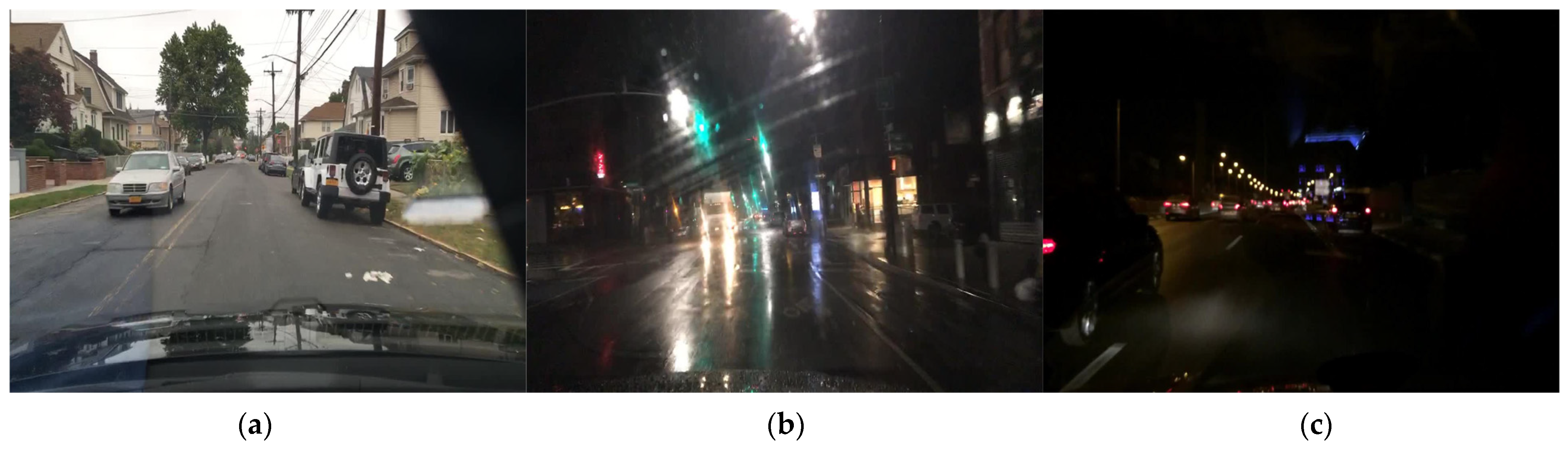
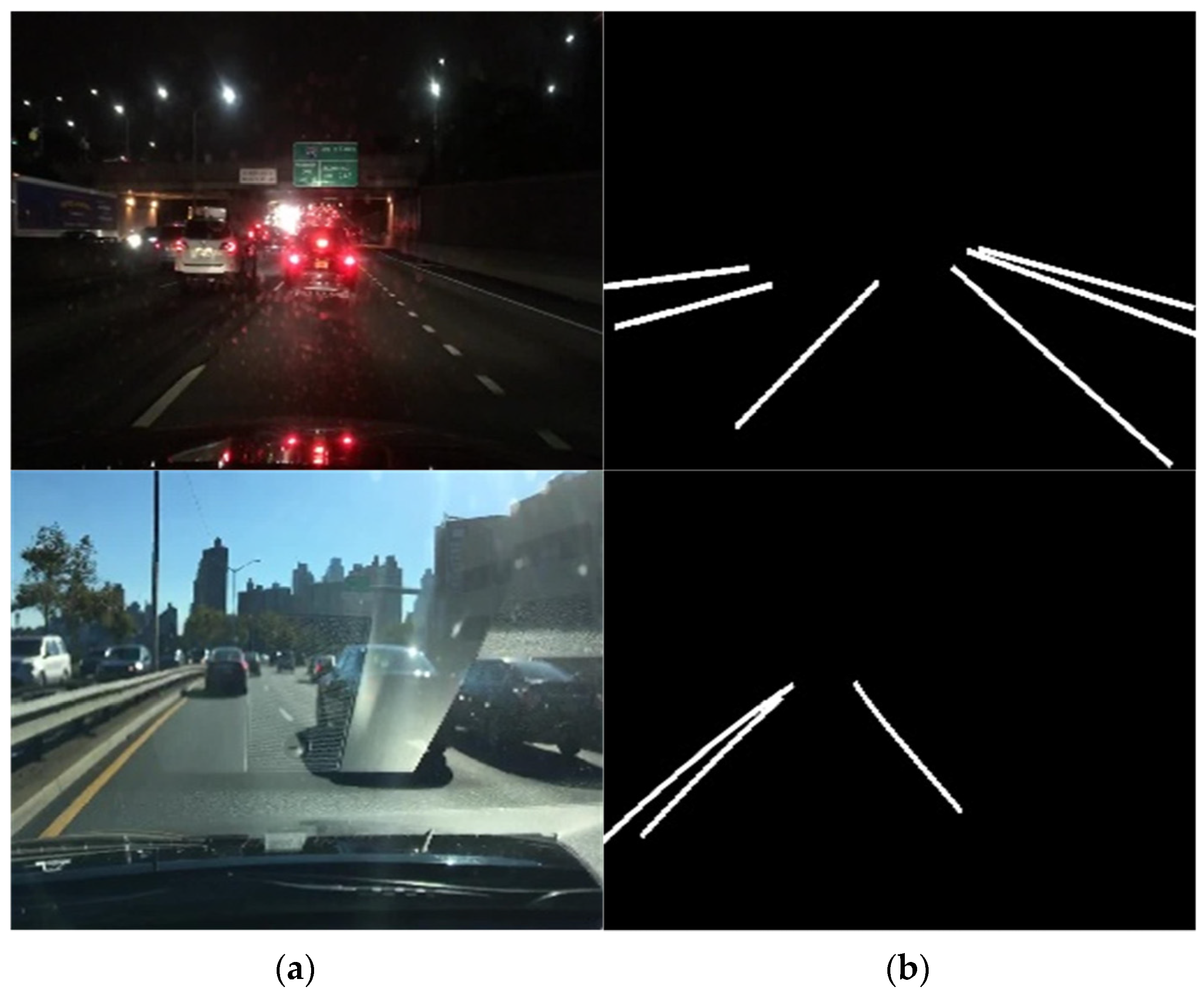
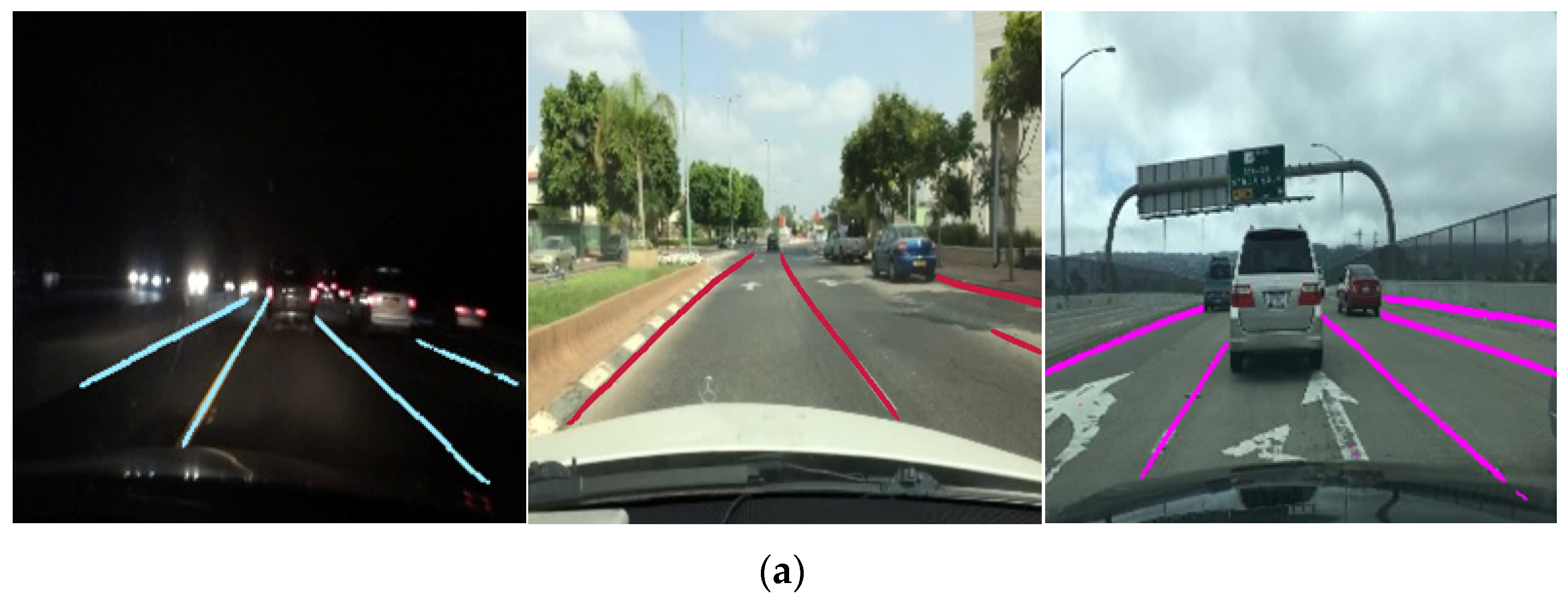
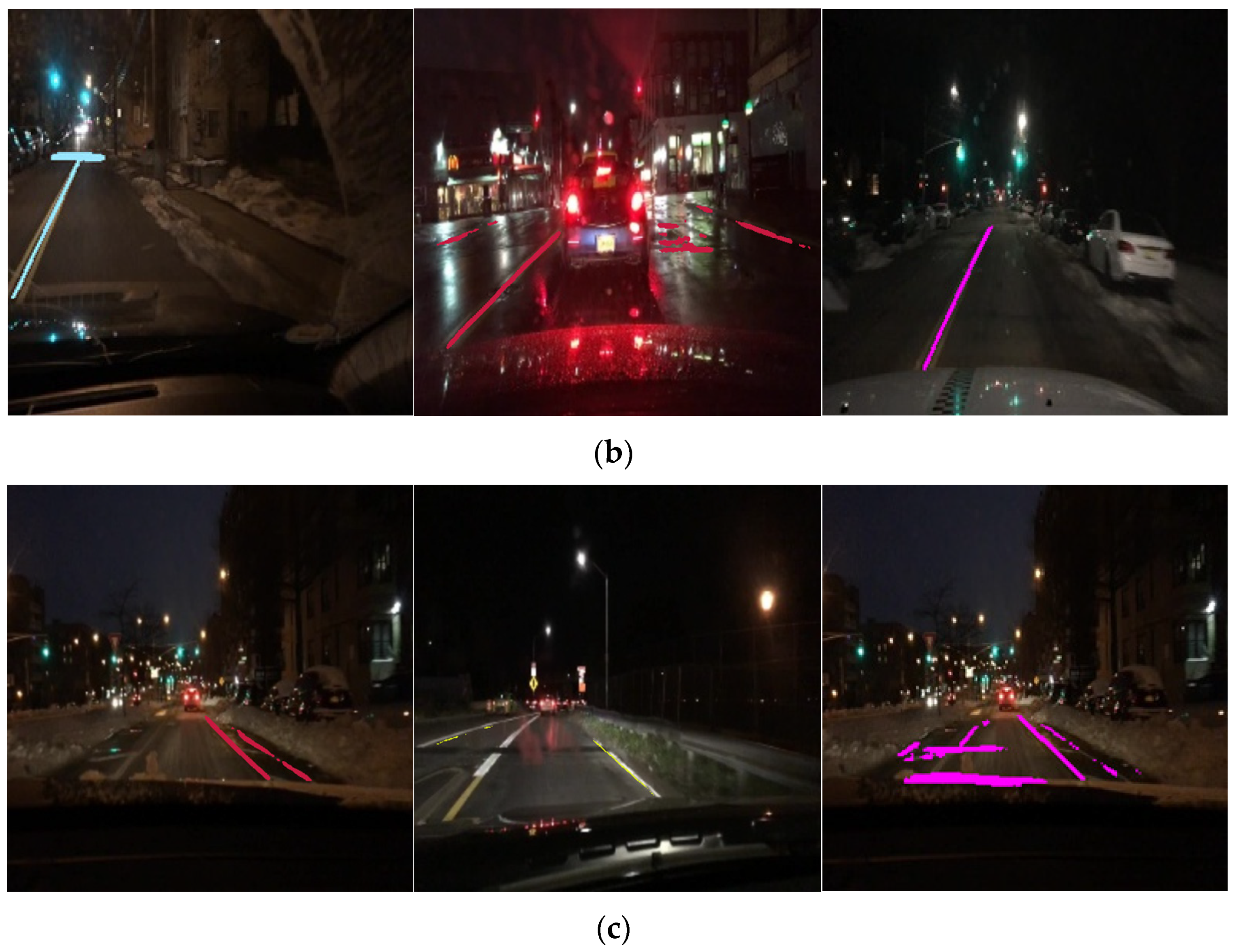
Autonomous driving systems primarily employ a range of sensors, including cameras and Lidar. Cameras are used to detect and analyze various elements (such as lanes, vehicles, and pedestrians) from captured images. In contrast, Lidar is used to perceive and assess driving situations by capturing distance information within the surrounding environment. Cameras are mainly used due to their relatively low cost and widespread availability, meaning image-based ADASs are more prevalent. However, market expansion has meant that ensuring reliable lane detection in diverse countries and environments has become a challenging task. Figure 1 demonstrates the diversity in road conditions, temporal and meteorological-dependent variables, and the heterogeneous driving environments observed across different nations. These intricate factors pose obstacles to reliable lane detection.

Figure 1.
Various environments during driving: (a) lane marking is severely deteriorated; (b) lane markings are nearly erased due to rainwater; (c) lighting conditions are insufficient, making the lane markings barely visible.
Recently, numerous approaches have been introduced that employ camera images for lane detection. In particular, deep learning algorithms have garnered significant attention following the success of AlexNet in the ImageNet competition, resulting in the widespread adoption of lane detection using trained models based on this CNN architecture [1,2,3,4]. In this study, lane detection methods are primarily categorized into two types: heuristics-based lane detection methods that predate the introduction of CNNs, and methods that apply CNNs. The heuristic-based methods mainly involve detecting lanes using empirical rules or expert knowledge. However, during vehicle operation, various environmental factors should be considered, because certain elements (such as fog, nighttime conditions, vehicle headlights, and lighting from other vehicles) and factors (such as taillights) can impede image-based lane detection. To mitigate these influences, techniques such as filtering, color space transformations, and region-of-interest delineation are employed [5]. Lane detection using CNNs includes the image-to-image approach, where an autoencoder learns from a segmentation map as the target [6]. Here, the U-Net architecture adopts a strategy that minimizes information loss by connecting the encoder and decoder through Skip connections [7]. Das et al. proposed a method utilizing a U-Net-based architecture to detect driver drowsiness by monitoring the state of the driver’s eyes, thereby enhancing road safety [8]. Additionally, a method utilizing YOLO has been developed that treats lanes as single objects for detection [9]. Furthermore, a stable training method has been proposed that uses generative adversarial networks (GANs), which are typically used for image generation, to reduce complex post-processing in semantic segmentation problems [10].
In this study, an algorithm that focuses intensively on learning the lane regions for various driving conditions is proposed. Detecting lanes that are obscured due to lighting or obstacles is a challenging task. However, this problem can be addressed by inputting additional edge information on the lanes being driven during training and focusing on learning them during loss calculations. Furthermore, refining the training data and adjusting the module structure enable stable learning. To summarize, our study adds the following important contributions:
- To train a modified U-Net architecture for detecting lane markings in the driving area through setting up a custom dataset.
- To remove unnecessary information from images and extract only the required data through data preprocessing.
- To ensure the robustness of loss calculation and to reflect information across different tasks, weight maps are assigned to areas where lane markings may potentially exist during the calculation of the loss function, while dynamic hyperparameters are incorporated into the loss function.
- To demonstrate the learning safety and usability of the proposed method, we validate it through ablation experiments and comparison experiments.
In the remainder of this paper, related research is introduced in Section 2, and the proposed method is explained in detail in Section 3. Section 4 demonstrates the effectiveness of the proposed method through comparative experiments with other approaches. Finally, Section 5 presents the summary, improvements, and future research directions.
2. Related Works
To achieve stable autonomous driving, various challenges need to be addressed, such as detecting obstacles, pedestrians, and lanes. Research on lane detection from images obtained through cameras mounted on vehicles started in the 1990s [11,12]. Since AlexNet’s triumph in the ImageNet competition, deep learning algorithms have been recognized as promising tools, resulting in the widespread adoption of lane detection using models trained with CNN architectures. Lane detection methods can be broadly divided into heuristic- and CNN-based techniques.
2.1. Heuristic-Based Lane Detection
Heuristic-based lane detection methods are primarily employed in traditional computer vision techniques, where detecting lanes is based on empirical rules or expert knowledge. One of these methods is the Hough transform, which is a technique for detecting geometric shapes in images. It detects lines by mapping them from the coordinate space to the parameter space [13] and is commonly applied under the assumption that most lanes consist of straight lines. However, not all lanes are straight. To address this problem, research has been conducted on addressing the curved shapes of lanes. Ding et al. [14] proposed a method for detecting curved lanes using a bird’s-eye view. Additionally, Duong et al. [15] suggested segmenting curves into straight lines from a microscopic perspective and applied the Hough transform to detect the lanes. Another approach was presented by Wang et al. [16], who used the Catmull–Rom spline to form arbitrary shapes through control points, describing a wider range of lane structures to detect curved lanes. Another method was based on the B-snake for lane detection and tracking algorithms, where arbitrary shapes were formed by a set of control points of a B-Spline to explain the lane structure [17]. In addition, Jung et al. [18] proposed a method for tracking curved lanes using a linear parabolic lane model.
Since vehicle-mounted cameras are exposed to the external environment, they can be susceptible to water droplets forming on the lens surface (due to rain or humidity) and contamination from dust. Moreover, images captured during driving can exhibit irregular lighting components and significant glare due to the vehicle’s headlights and taillights. These internal and external camera issues contribute a considerable amount of noise in the captured images. Srivastava et al. [19] proposed an effective noise removal method for lane detection using Median, Wiener, and hybrid filters. Wang et al. [20] suggested restricting the road area to the Region of Interest (ROI) and improving image quality through histogram equalization. ROI identification involves blocking out non-road information before enhancing poor lighting conditions through image processing. Javeed et al. [21] proposed detecting lanes using the ROI and Otsu’s method, while Yeongho et al. [22] suggested blocking out factors due to unnecessary lighting in the ROI using adaptive thresholding, leaving only lane information. The images acquired during driving are prone to color distortion due to the headlights and taillights of the vehicle and noise from the camera. By converting from RGB to a different color space and performing image processing, such distortion can be prevented. Lee et al. [23] proposed a method of preventing distortion by converting RGB to the CIELab space and then separating only the luminance channel for image processing. Lane markings are typically displayed in clear white or yellow colors on dark road backgrounds to ensure visibility in the driver’s line of sight. By employing this characteristic, the boundaries of lanes can be extracted through Sobel and Canny edge filters [24]. Alternatively, there are lane detection methods that use algorithms such as RANSAC to build mathematical models based on pixel positions as datasets [25]. After detection, lanes are usually tracked on a frame-by-frame basis. One of the representative lane tracking techniques involves the use of the Kalman filter, which recursively corrects the estimated value of the current state based on the predicted value of the previous state, allowing real-time lane tracking [26].
2.2. CNN-Based Lane Detection
Image-to-image learning is a prominent lane detection method based on CNNs that generates a segmentation map from driving images. This approach requires pairs of driving and label images that label the lanes from the driving images. U-Net is a method that uses this approach, connecting the encoder and decoder with skip connections to preserve information while detecting lanes [27]. Qin et al. [28] proposed a lane detection learning method by replacing U-Net’s skip connection with long short-term memory (LSTM), allowing finer control of information transmission from the encoder to the decoder when detecting lanes. Lee et al. [29] suggested a real-time lane detection method that replaced U-Net’s convolution layer with a Depthwise separable convolution layer, reducing the number of parameters used in training and achieving a lightweight structure. Feng et al. [30] proposed a lane detection method using ResNet, which is similar to U-Net and prevents information loss during backpropagation through skip connections between the encoder and decoder. However, unlike U-Net, ResNet does not decrease or increase the size of the input data in the encoder and decoder. Another approach is to find drivable areas instead of lanes, which involves using a segmentation map of drivable regions as the label image instead of a segmentation map of the lanes. Lyu et al. [31] proposed a method for segmenting road areas by training with distributed LSTM layers instead of convolution layers. Another approach involves treating lanes as objects rather than segmentation and then detecting them as objects. Xiang et al. [9] proposed a method that uses YOLO v3 to treat lanes as objects, which are then detected. Another approach involves using a generative adversarial network (GAN). Mohsen et al. [10] used Embedding Loss GAN (EL-GAN) to make the output of semantic segmentation networks more realistic and structurally preserved. This approach enhances the similarity between the actual labels and the output, simplifies the post-processing stage, and achieves higher accuracy.
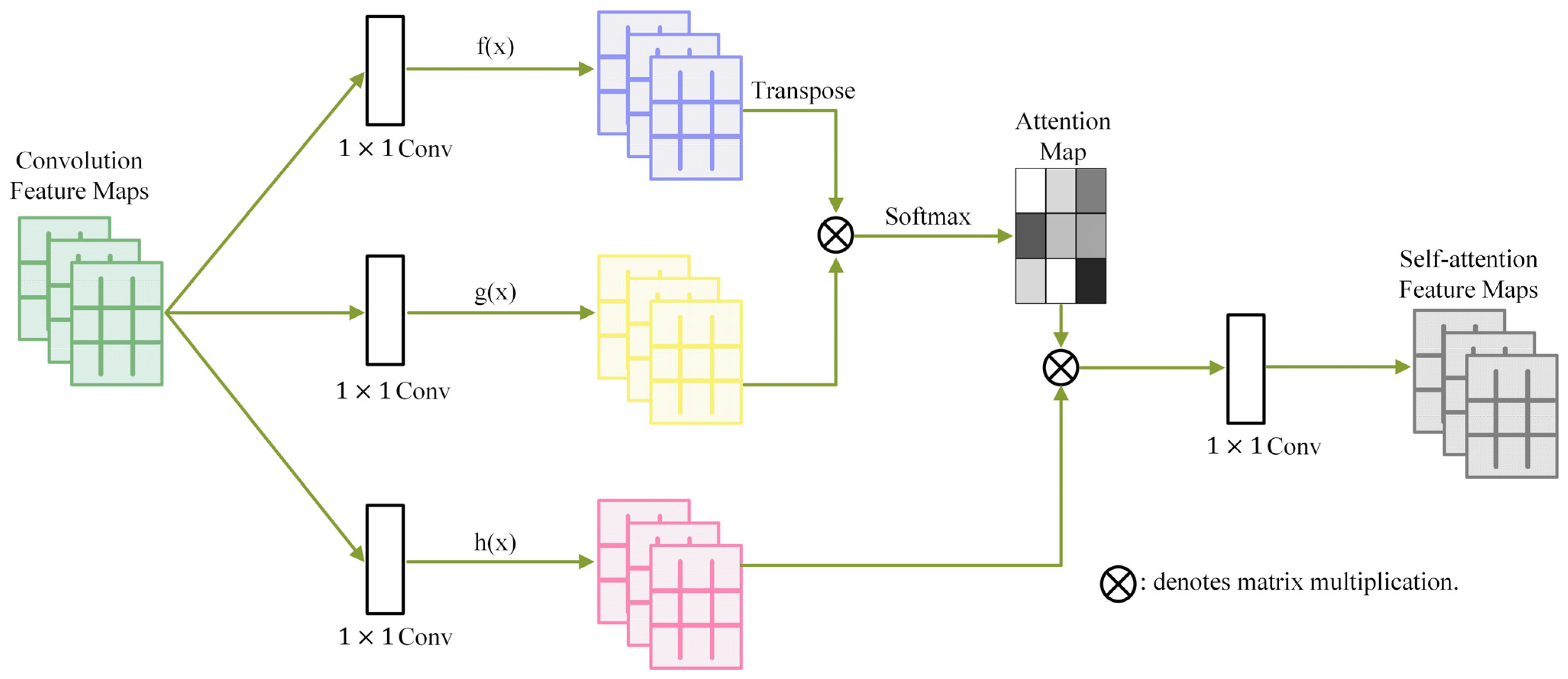
An attention map visually represents the model’s focus level on given inputs and is used in deep learning models to concentrate on specific parts or emphasize features. The attention mechanism has the potential to enhance the detection performance of modules [32]. Li et al. [33] generated an attention map associated with prediction results to focus on the most important parts of the image. They also designed a spatial feature transformer (SFT) to extract discriminative features from the attention map and proposed a new dual-channel CNN architecture for fusing features extracted from the RGB stream and attention map. Zhang et al. [34] proposed a learning model called self-attention GAN, which adds structure to modules to focus attention on complex areas relevant to image generation tasks, increasing the efficiency of learning. In self-attention GAN, a CNN structure is added to create the attention map, as illustrated in Figure 2. Here, f(x) and g(x) represent different feature spaces, and h(x) is used to control the weights for synthesizing the attention map from f(x) and g(x). The research in this paper emphasizes the directional edge filter instead of feature maps created through training to generate an edge image highlighting the left and right lanes of the driving area for the attention map. These attention maps are then integrated into the input data of the training as the fourth channel, resulting in the creation of four-channel input data.
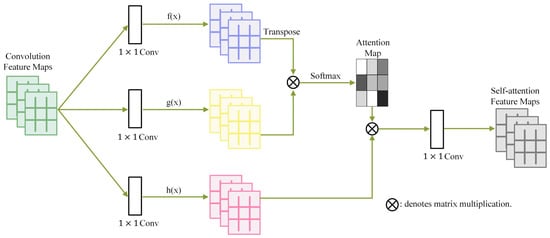
Figure 2.
Self-attention generative adversarial networks. (f(x), g(x), h(x): feature space).
3. Proposed Method
3.1. Overview of Proposed Method
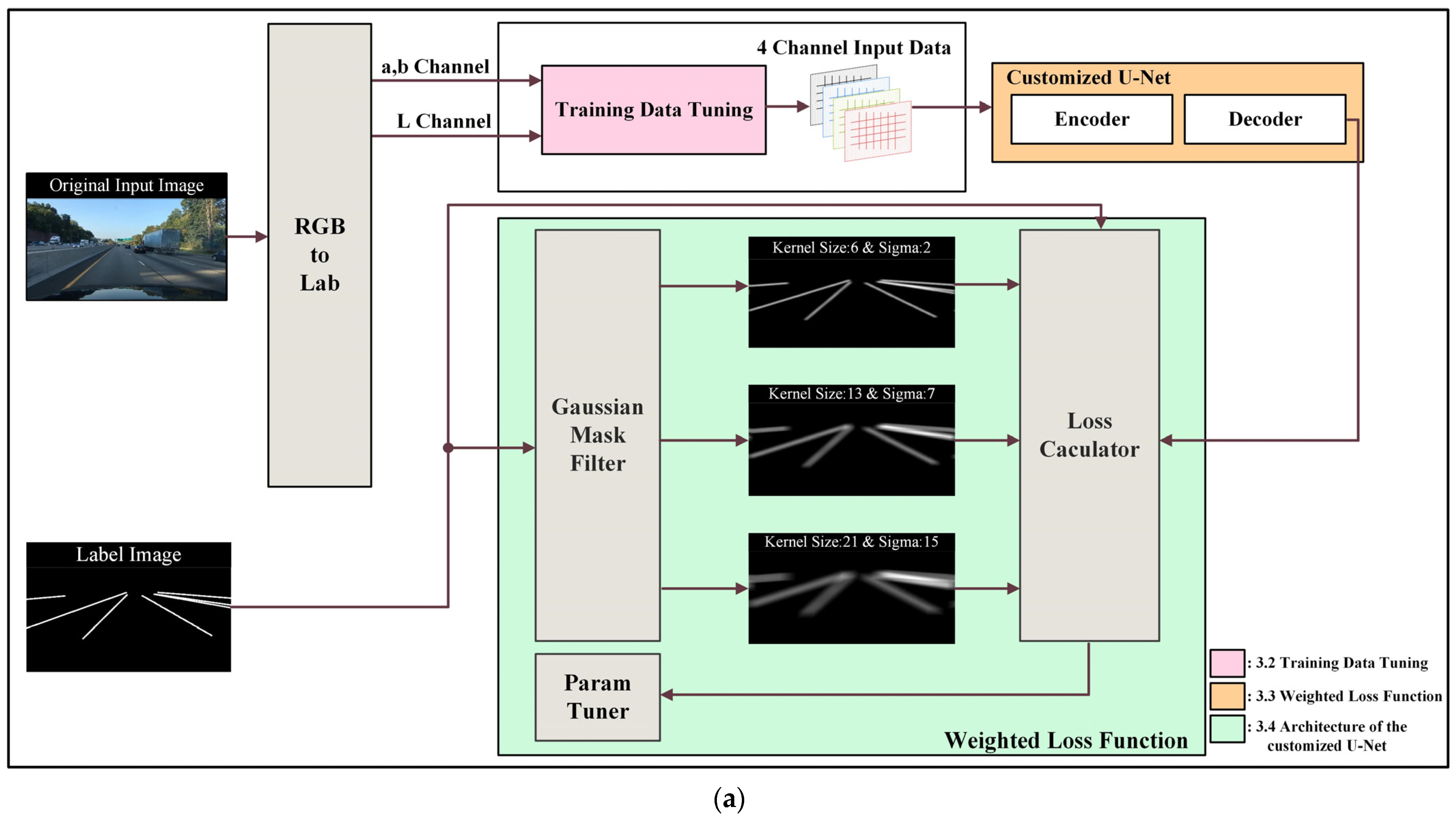
Figure 3 illustrates the overall process flow of the proposed learning algorithm. Figure 3a displays the entire structure, including preprocessing and post-processing for training, while Figure 3b presents the module structure used in training.

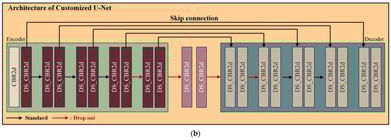
Figure 3.
Overview of flow chart: (a) framework of the proposed method, and (b) detailed structure of customized U-Net (L channel represent brightness, a channel represents the color between red and green, b channel represents the color between yellow and blue).
In this study, the Lab color space is utilized for preprocessing the training data. The luminance channel undergoes bilateral filtering and multiscale Retinex (MSR) processing to remove noise and enhance local contrast, resulting in an improved image. Additionally, a directional edge filter is applied to generate an edge index image that emphasizes the left and right lanes of the roadway area during driving. These processed images are then combined with the RGB image to create training input data that comprises four channels. Subsequently, the U-Net architecture is modified to accommodate the four-channel tensor, and an additional layer is added before and after the neck stage of the U-Net. However, adding these layers increases the parameter count by a factor of approximately four, resulting in issues such as overfitting, excessive memory usage, and increased training time. To address this problem, the standard convolution layer is replaced with the Depthwise separable convolution layer proposed by Francois et al. [35] to reduce the parameters. Additionally, dropout is employed to substitute for the input and output of the added layers to prevent overfitting. The loss comprises a total of four components: a binary cross-entropy (BCE) loss and three mean absolute error (MAE) losses. The weights of the loss are then adjusted using a param-tuner. Each subsequent section is explained block by block in the following order: Section 3.2—Training Data Tuning, Section 3.3—Weighted Loss Function, and Section 3.4—Architecture of Customized U-Net.
3.2. Training Data Tuning
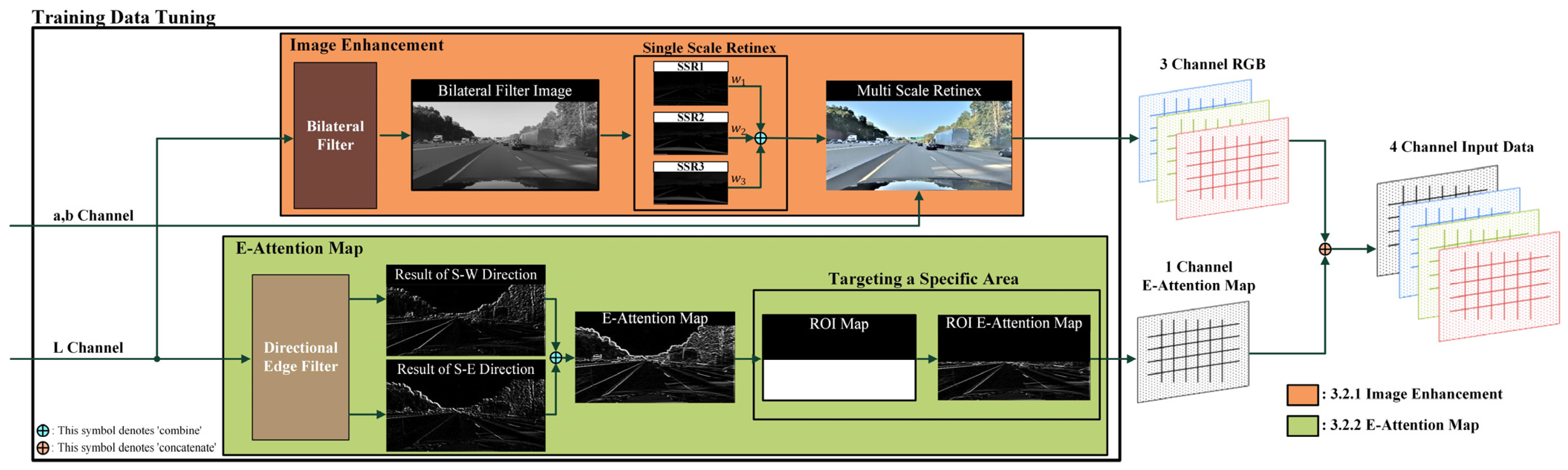
Data preprocessing for training is explained in Figure 4. The input data are transformed into the Lab color space. Moreover, by only using the luminance information while preserving the color information of image channels a and b, any loss in color information is minimized. The L channel input undergoes two main processes. The first involves removing noise, and lanes are highlighted to acquire the RGB image through bilateral filtering and the MSR process. In the second process, an attention map is generated to focus on lanes during training. The edge attention map (E-attention map) is formed by the directional edge filter and the ROI to establish the target lane of the road. The input data consist of three RGB channels and one directional edge image channel, which are combined to generate four-channel input data.
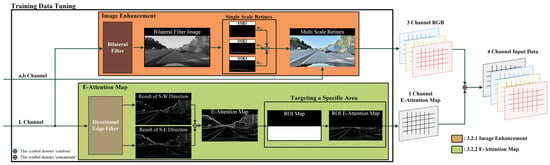
Figure 4.
Process of training data tuning (L channel represent brightness, a channel represents the color between red and green, b channel represents the color between yellow and blue).
3.2.1. Image Enhancement
The first image enhancement step involves applying a bilateral filter to the input L channel, removing noise while enhancing the local contrast of the lane with MSR. Unlike a Gaussian filter, the bilateral filter consists of two sigma parameters that can adjust the extent and range of applied blurring by using each range of sigma and spatial sigma. These characteristics can be understood by comparing the equations of Gaussian and bilateral filters.
where Equation (1) represents a two-dimensional Gaussian function, where denotes the probability density function for and . Terms and represent the standard deviations in the and directions, respectively, while and denote the means in the and directions. These parameters determine the width and height of the Gaussian function, controlling the degree of blur. Term represents the output value at position in the bilateral filter, where is a normalization constant ensuring that the total weight sum is 1. Terms and indicate the standard deviations for the spatial differences, with representing the difference between and , and representing the difference between and . Term is the standard deviation for brightness differences, representing the brightness variation between adjacent pixels. Adjusting this parameter determines the extent of the blur applied.
The bilateral filter has three adjustable parameters: the size of the kernel, the spatial sigma determining the degree of blur, and the range sigma (which controls the extent of blur). It is necessary to apply each sigma option differently depending on the time of day (i.e., day or night). The luminance information in the image allows for measuring the overall brightness of the scene. Lee et al. [23] proposed a method for determining the day and night in an image based on the measured average value, and then configuring parameters suitable for daytime and nighttime accordingly.
Applying Retinex theory to each sigma value to generate single-scale Retinex (SSR) images allows for obtaining optimized results that effectively suppress noise while minimizing contrast degradation. The concept of Retinex originates from the understanding that human vision is more sensitive to relative illumination than the overall background. When Gaussian blur is applied to the original image, only the background components remain. Subtracting these background components from the original image extracts the relative illumination component. After undergoing this process for each Gaussian sigma value, multiple SSR images are generated, which are then combined into a single multiscale Retinex image with weighted fusion. This process is illustrated in Equations (3) and (4).
where represents the SSR value of image , denoting the corrected brightness value of each pixel, while represents the pixel value of the input image, where indicates the coordinates of the image. Moreover, denotes the natural logarithm value of the pixel value of the input image, while represents the spatial weight, which comprises a Gaussian filter that is used to smooth the brightness around the pixel. Finally, computes the spatial average for each pixel of input image , obtaining the illumination component by subtracting it from the original image. After multiplying the calculated single-scale by each weight and summing them, an MSR image is generated. The synthesized L-channel MSR image is then combined with the preserved a and b information and converted from the Lab space to the RGB color space. The detailed image enhancement procedure is shown in Algorithm 1.
| Algorithm 1 Image Enhancement |
| 1: Input: 2: Initialize: 3: 4: 5: for do 6: 7: 8: end for 9: Output: |
3.2.2. E-Attention Map and Targeting a Specific Area
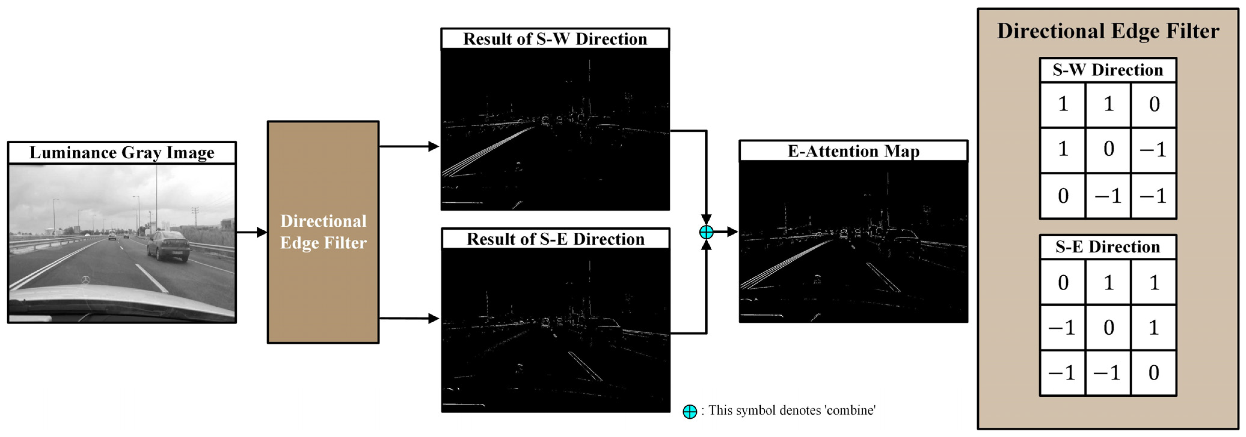
To some extent, it is possible to predict the angle of the lane lines in the road area where the vehicle is currently driving from the camera installed on the vehicle [23]. Accordingly, we set up filters to extract only the edge information of the lane lines in a specific direction (the directional edge filter) to emphasize both the left and right lane lines. Using this designed directional edge filter, edge images emphasizing the left and right lane lines are generated separately and then combined into one image through normalization and summation. The entire process is illustrated in Figure 5.
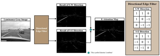
Figure 5.
The process of creating an E-attention map using a directional edge filter.
The generated edge images only retain information about the road area, while the sky area is considered unnecessary and is removed entirely using the ROI. Subsequently, these edge images are incorporated as the fourth channel of the RGB image generated in the first step, resulting in the final creation of four-channel input data. The detailed procedure is shown in Algorithm 2.
| Algorithm 2 E-Attention Map and Targeting a Specific Area |
| 1: Input: , 2: for do 3: for do 4: 5: 6: end for 7: end for 8: 9: = 10: 11: Output: |
3.3. Weighted Loss Function
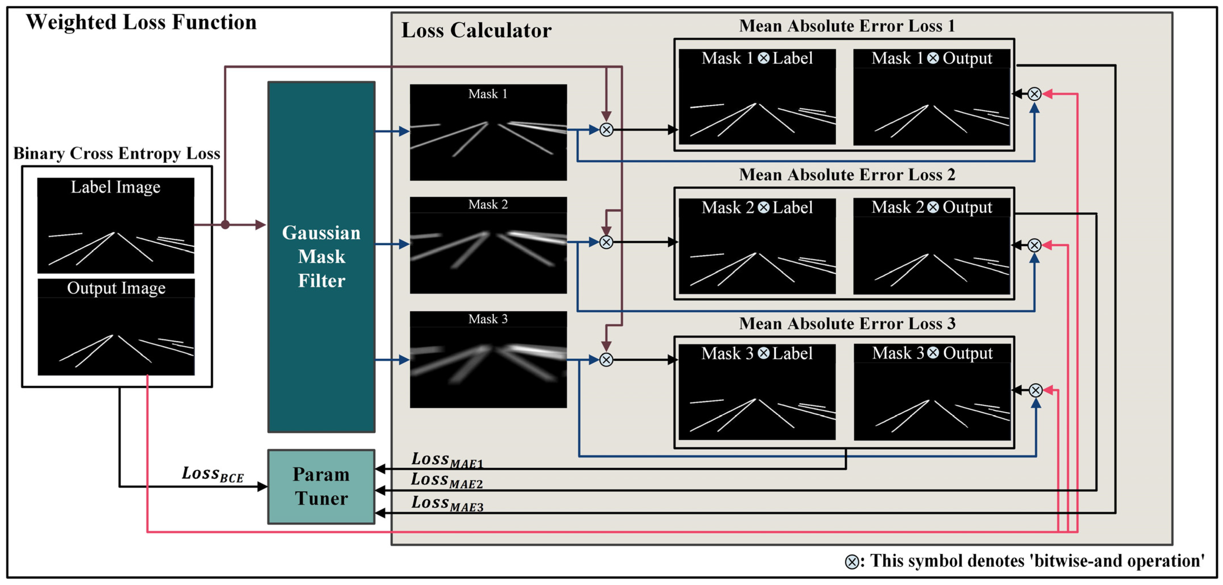
Comparing regions where the likelihood of lane absence is high could degrade the performance of the loss function. Therefore, we propose a method to enhance lane detection accuracy by introducing a weighted map with Gaussian-filtered loss functions. The aim is to facilitate more precise training by adding information about potential lane areas to the label image during training. Specifically, Gaussian masks with different sigma values are applied to the label image to highlight areas where lanes could exist. During loss function computation, individual loss terms for each blurred label image are calculated separately and treated as separate loss functions. The sigma values of the Gaussian filters are used differently to induce the model to learn various levels of lane information, helping to focus on local details and capture the lanes more effectively.
As illustrated in Figure 6, the process involves using Gaussian masks with different sigma values that are generated from the label image through the Gaussian mask builder. These masks (denoted as Gaussian masks 1, 2, and 3) are employed to compute various MAE losses between the model’s output image and the original label image. Additionally, BCE losses are computed from the original label image and output image, and all adjusted loss functions are processed through a parameter tuner.

Figure 6.
Process of weighted loss function (Mask 1: kernel size 6 and sigma 2; Mask 2: kernel size 13 and sigma 7; Mask 3: kernel size 21 and sigma 15).
Four loss functions are employed in this process. The binary cross-entropy (BCE) loss is applied to the original label image and the output image, while the mean absolute error (MAE) loss is used for the label image with the Gaussian filter applied and the output image. The BCE loss is commonly used in binary classification problems for measuring the difference between the output image and the target label image, considering whether a pixel value exists at a given location. In contrast, the MAE loss computes the absolute difference between the predicted and ground truth values for each sample. This is calculated for the result passed through the Gaussian mask, considering the potential positions of the lanes, by summing the differences for all samples and then computing the average. Equations (5) and (6) represent these two processes.
where refers to the BCE loss function, N represents the total number of data points, and represents the actual label, indicating the actual label of each data point in binary classification as either 0 or 1. Term represents the probability of the label being 1 predicted by the model for each data point. The BCE loss function calculates the error between the model’s predicted values and the actual values for each data point. The model is trained in the direction of minimizing this error. Term refers to the MAE loss function, where N represents the total number of data points, represents the actual label, and represents the probability of 1 being predicted by the model. The MAE loss function measures the absolute error between the actual and predicted values for each data point and averages the errors over all data points.
where represents the loss between the output predicted by the model and the target label, which is set as an exponentiated value of the exponential function. Terms and represent the loss between the label passed through the Gaussian masks according to each sigma value and the output, which are set as exponentiated values of the exponential function. This is designed to accelerate learning based on the softmax function. The parameter tuning formula adjusts the terms where the loss is small to be more heavily weighted during the loss calculation, while terms where the loss is high are weighted less. Parameter adjustment can accelerate learning to some extent. The detailed procedure is shown in Algorithm 3.
| Algorithm 3 Weighted Loss Function |
| 1: Input: 2: 3: for do 4: 5: 6: 7: end for 8: 9: 10: 11: Output: |
3.4. Architecture of the Customized U-Net
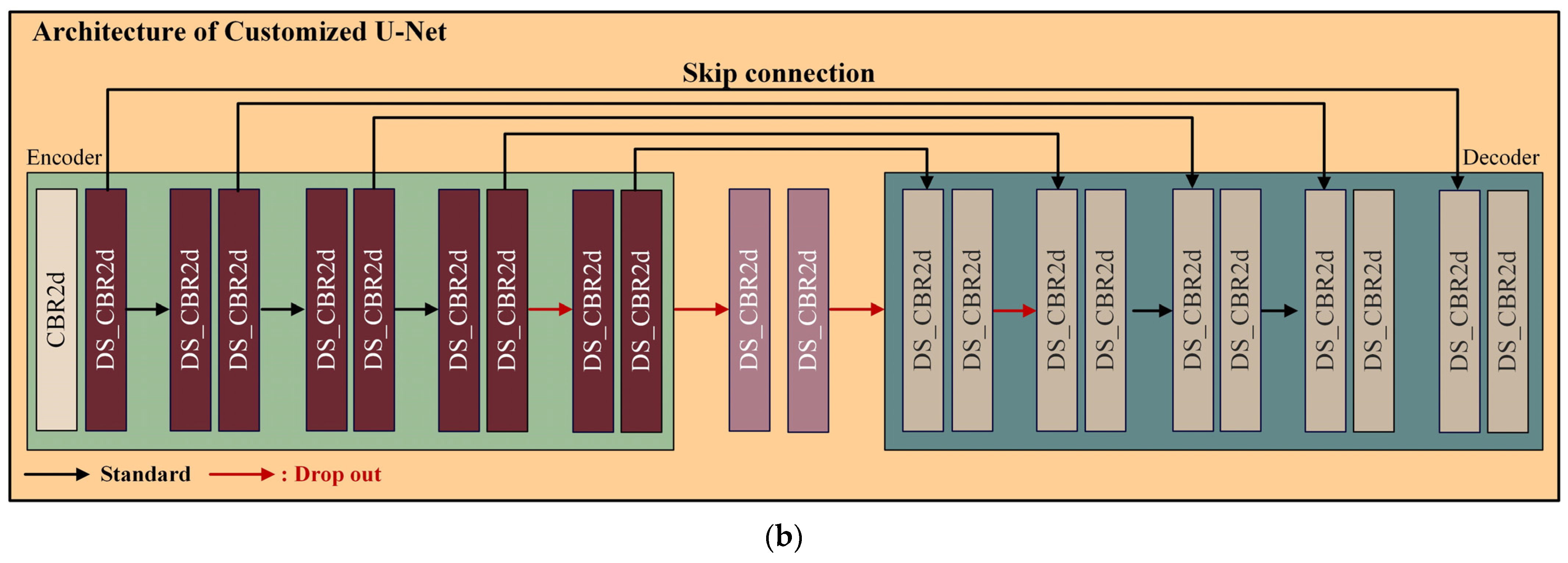
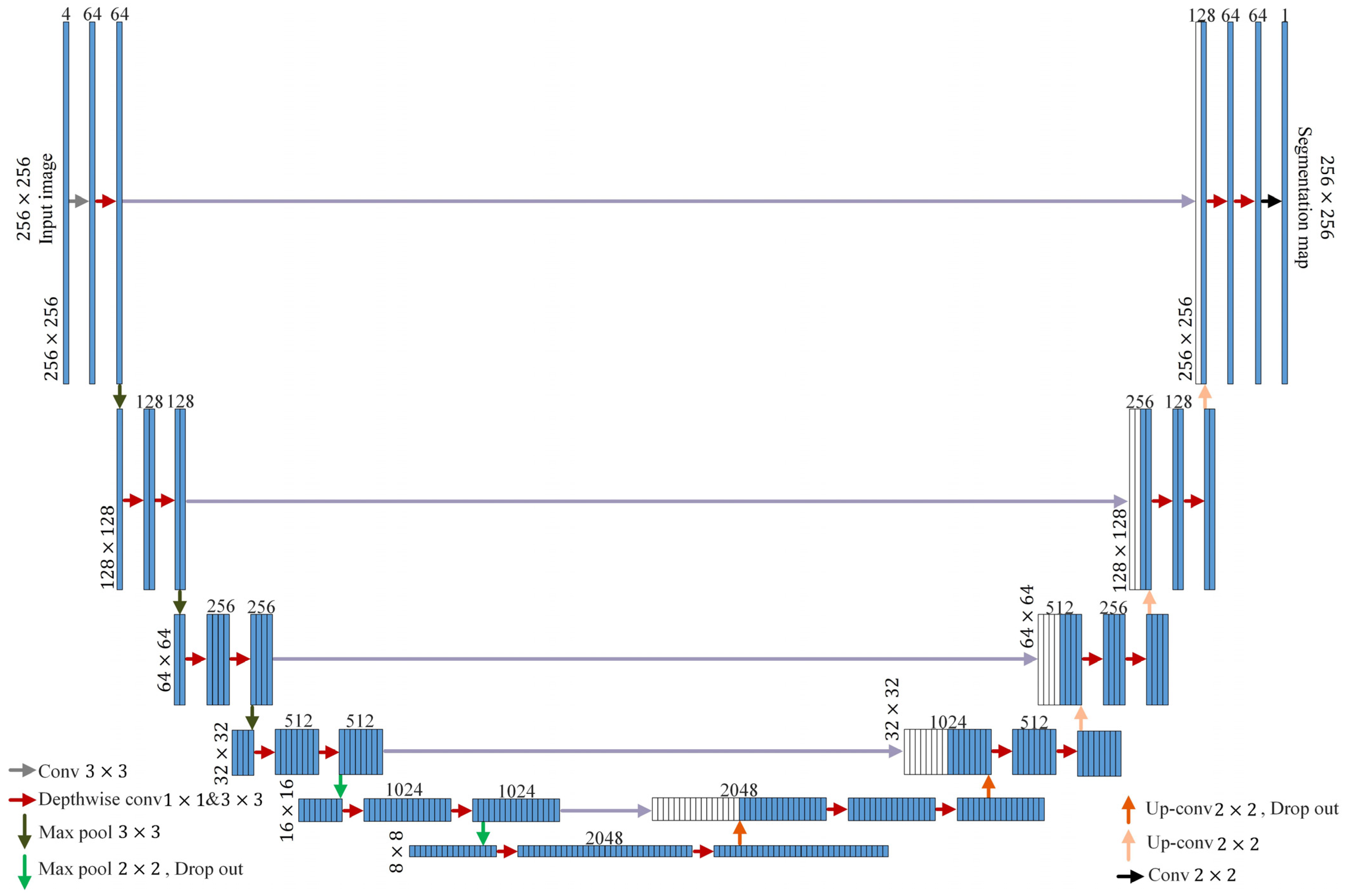
In this paper, training is conducted based on U-Net. The 4-channel input data require a larger amount processing compared to the 3-channel input data. To process the four-channel input data effectively, each layer in the encoder and decoder of the original U-Net is augmented by one layer. An additional layer was added to the encoder part just before entering the neck, and similarly, an extra layer was added to the decoder immediately after coming out from the neck. Adding just one layer significantly increases the number of parameters to be trained nearly fourfold. Therefore, as the structure becomes deeper with added layers, overfitting can occur. As the layers deepen, the phenomenon of gradient vanishing occurs, and as the number of parameters to be trained increases, optimization only occurs in the training data. To mitigate this problem, the inputs and outputs of the additional layers are replaced with dropout. Dropout is a regularization technique in neural networks aimed at reducing overfitting by randomly removing some neurons during training. This can reduce network dependency and improve generalization performance. Furthermore, increasing the number of parameters extends the training time and requires more memory. Therefore, it is necessary to reduce the number of parameters while minimizing performance degradation. Depthwise separable convolution was proposed by Francois et al. [35] to accomplish this aim. Figure 7 illustrates the modified U-Net structure.
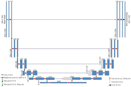
Figure 7.
Architecture of customized U-Net.
4. Experiments and Results
4.1. Settings
The performance validation experiments for the proposed approach were conducted in two parts. The first experiment involved optimizing the parameters of the proposed modules and demonstrating the efficiency of each block by applying the modules to individual blocks. In the second experiment, the proposed method was compared with different approaches to showcase its efficiency. For the training, a randomly selected subset of 30,000 images was used from the BDD100k dataset. All the training images were resized to 256 × 256. Figure 8 illustrates the input and label pair data used for the training. The test was conducted using both the BDD100k dataset, which was not used in the training samples, and data directly captured by a camera model named 99250AR010, which provides FHD quality. The options for the modules used in training were consistent across all cases: batch size = 24, epoch = 120, and a learning rate of 2 × 10⁻⁴. The training and experiments were implemented on an RTX 4090 GPU (Nvidia, Santa Clara, CA, USA) and an i7-13700 CPU (Intel, Santa Clara, CA, USA).

Figure 8.
Training data pair set: (a) RGB scene data and (b) label data.
4.2. Evaluation Metric
First, we describe the evaluation method for lane detection. The aim of this study was not to create a segmentation map identical to the label data. The objective was to detect the lanes in the roadway area where the vehicle was driving. To achieve this, unnecessary information was restricted and only essential information was injected into the training. Therefore, evaluating the difference between the label image and the output image in terms of true positive, false positive, and false negative would not align with the goal of this study. Only the lanes in the driving area were considered for evaluation. Figure 9 illustrates cases where both the left and right lanes were accurately detected, as well as cases where only the left or right lane was accurately detected.
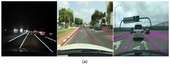

Figure 9.
Example of ground truth for evaluation criteria: (a) both lanes’ detection, (b) left lane detection, and (c) right lane detection.
4.3. Ablation Experiments for Option Adjustment
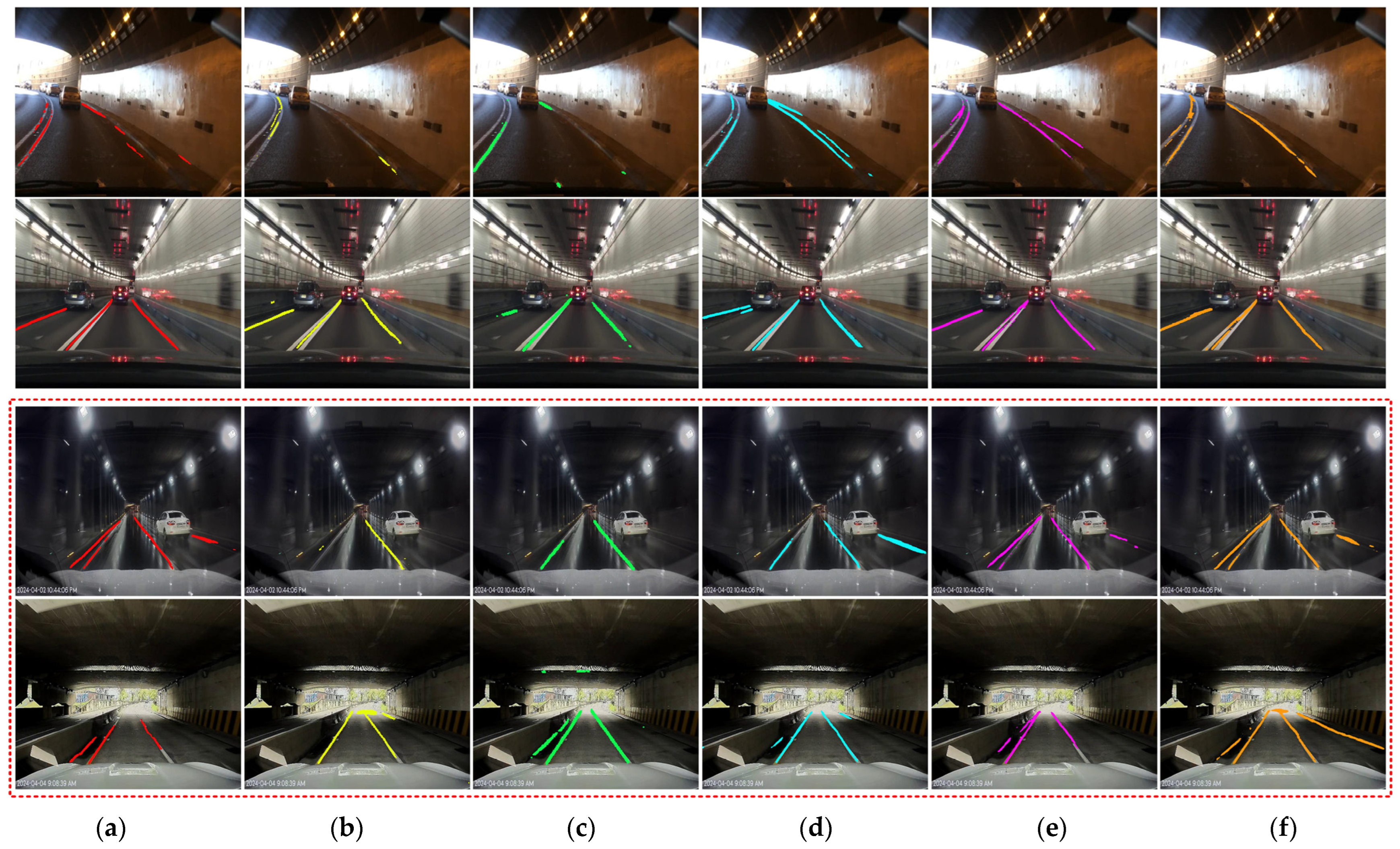
In this section, blocks were progressively applied to test the performance of each block. The experiment was defined through six cases. Case 1 represents the result where all the proposed blocks are applied. Case 2 involves training with 3-channel input data instead of 4-channel input data to validate the effectiveness of the 4-channel input data. Case 3 involves comparing with the case where lane direction is not considered, using the Sobel filter instead of the directional edge filter to generate the 4th channel edge image. Case 4 uses a simple vertically and horizontally separated ROI weight map instead of the loss weight map to demonstrate the effectiveness of the Gaussian mask builder. Case 5 involves uniformly combining and , and without weighting to demonstrate the effectiveness of the param-tuner. Case 6 involves the numerator of beta1 and beta2 being exchanged in the param-tuner to determine whether the training will be accelerated or decelerated when the weights are determined. By conducting experiments in various environments, the reliability of the experiments is increased. The experiments are conducted in five scenarios, each comprising 100 images: (1) daytime conditions; (2) conditions where lane detection is challenging due to reflections from sunlight or rainwater; (3) nighttime conditions; (4) conditions where lane detection is challenging due to reflections from other vehicles, streetlights, or billboards during the night and rainy conditions; and (5) indoor environments such as bridges and tunnels. Table 1 presents the detection rate. Figure 10, Figure 11, Figure 12, Figure 13 and Figure 14 illustrate the results of each case.

Table 1.
Evaluation table.
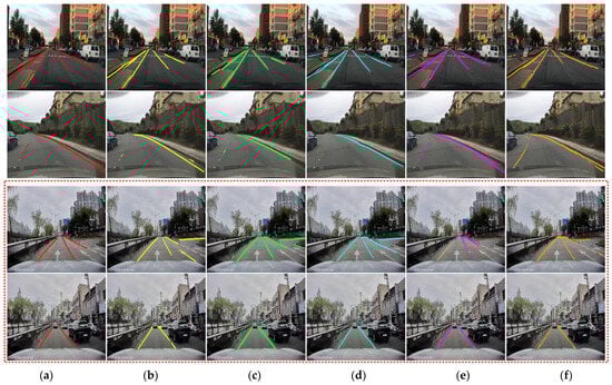
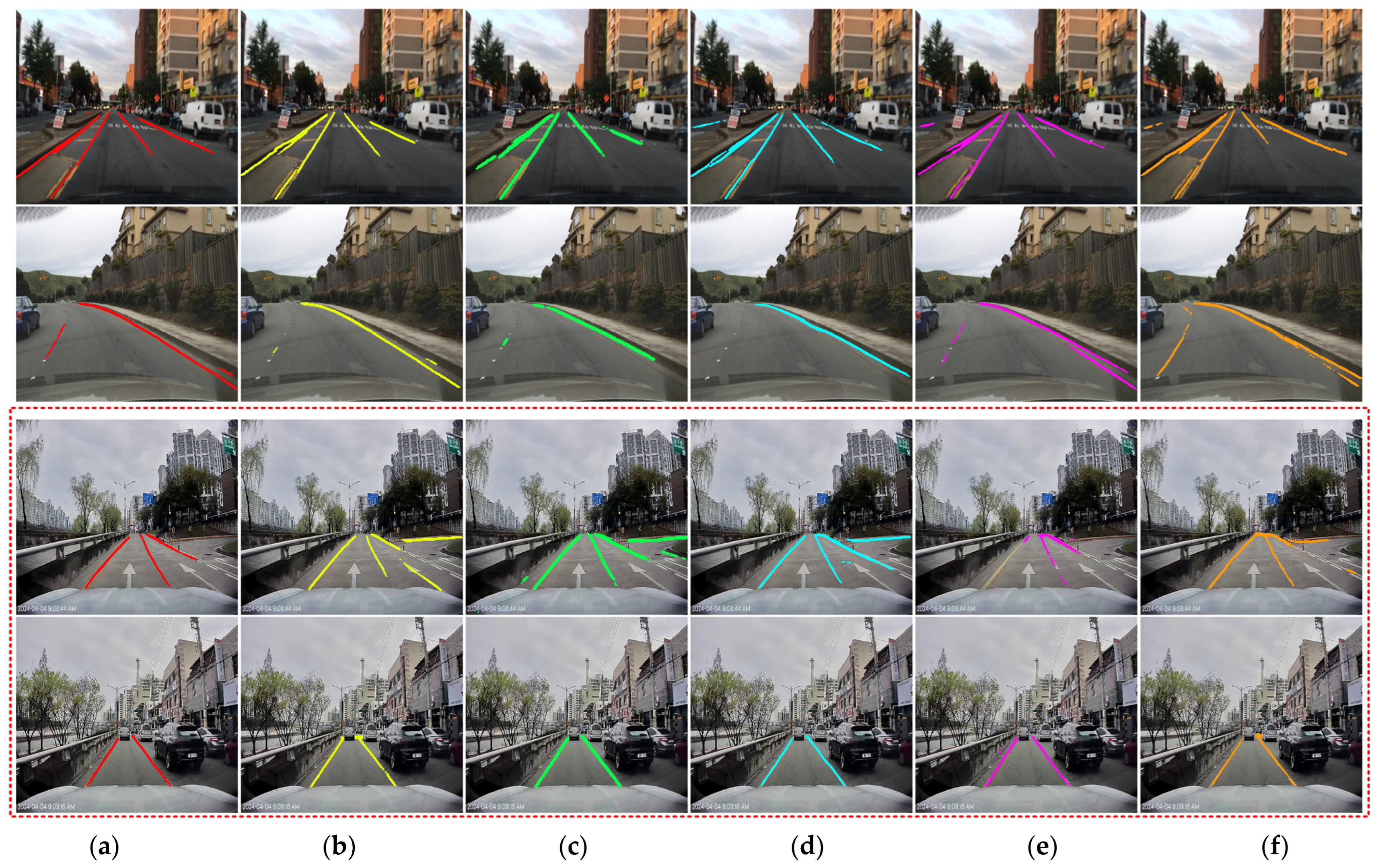
Figure 10.
The result of the evaluation in scenario 1 (the red dotted box represents the Lab. dataset): (a) proposed method (Case 1), (b) Case 2, (c) Case 3, (d) Case 4, (e) Case 5, and (f) Case 6.
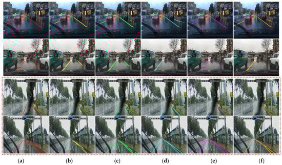
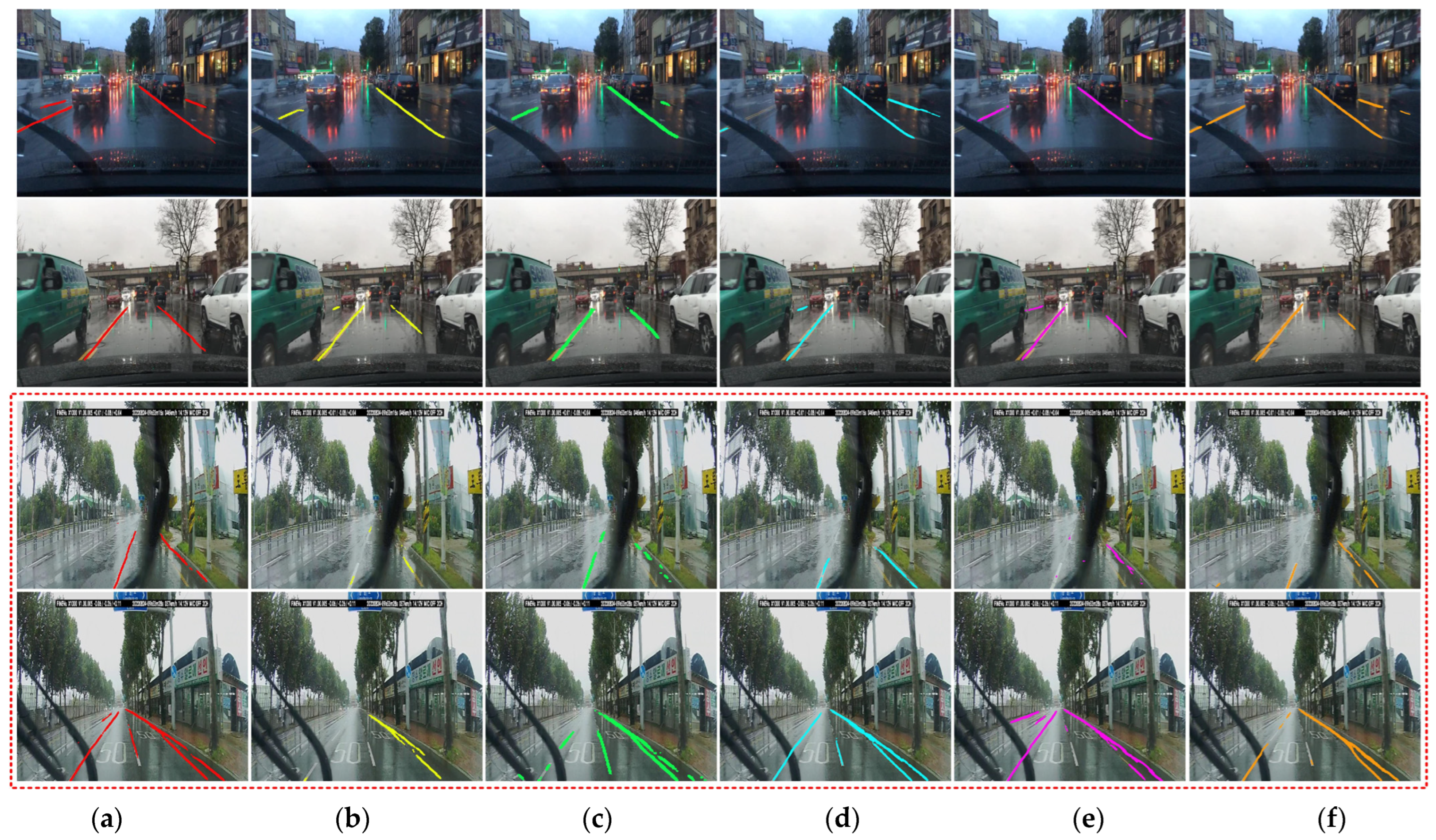
Figure 11.
The result of the evaluation in scenario 2 (the red dotted box represents the Lab. dataset): (a) proposed method (Case 1), (b) Case 2, (c) Case 3, (d) Case 4, (e) Case 5, and (f) Case 6.
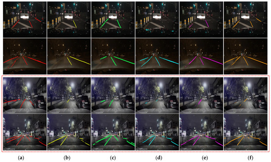
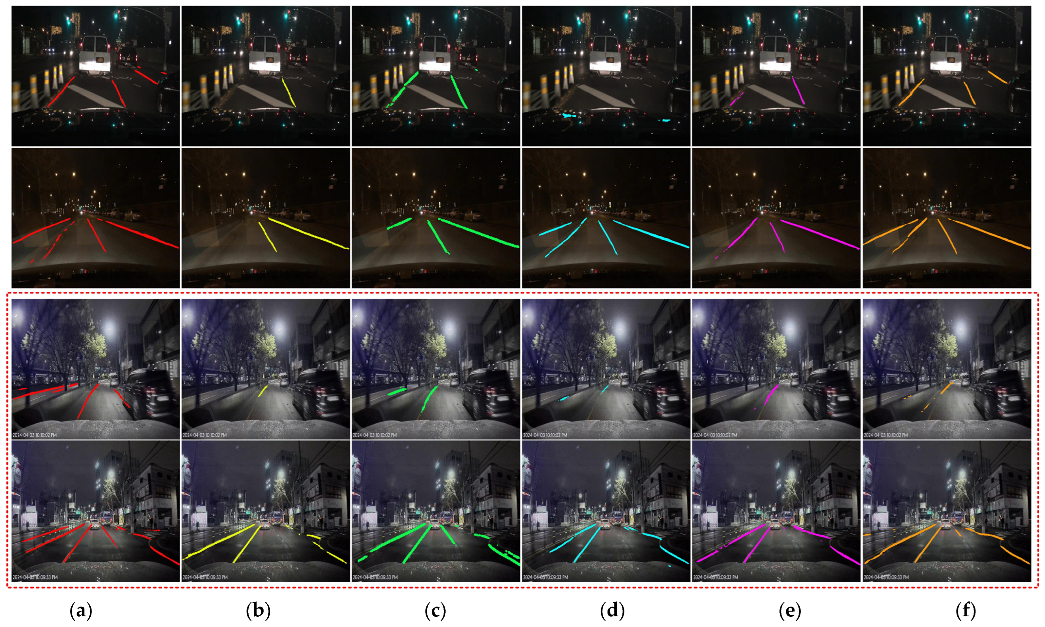
Figure 12.
The result of the evaluation in scenario 3 (the red dotted box represents the Lab. dataset): (a) proposed method (Case 1), (b) Case 2, (c) Case 3, (d) Case 4, (e) Case 5, and (f) Case 6.
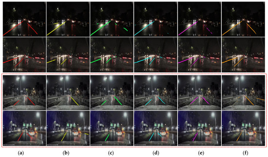
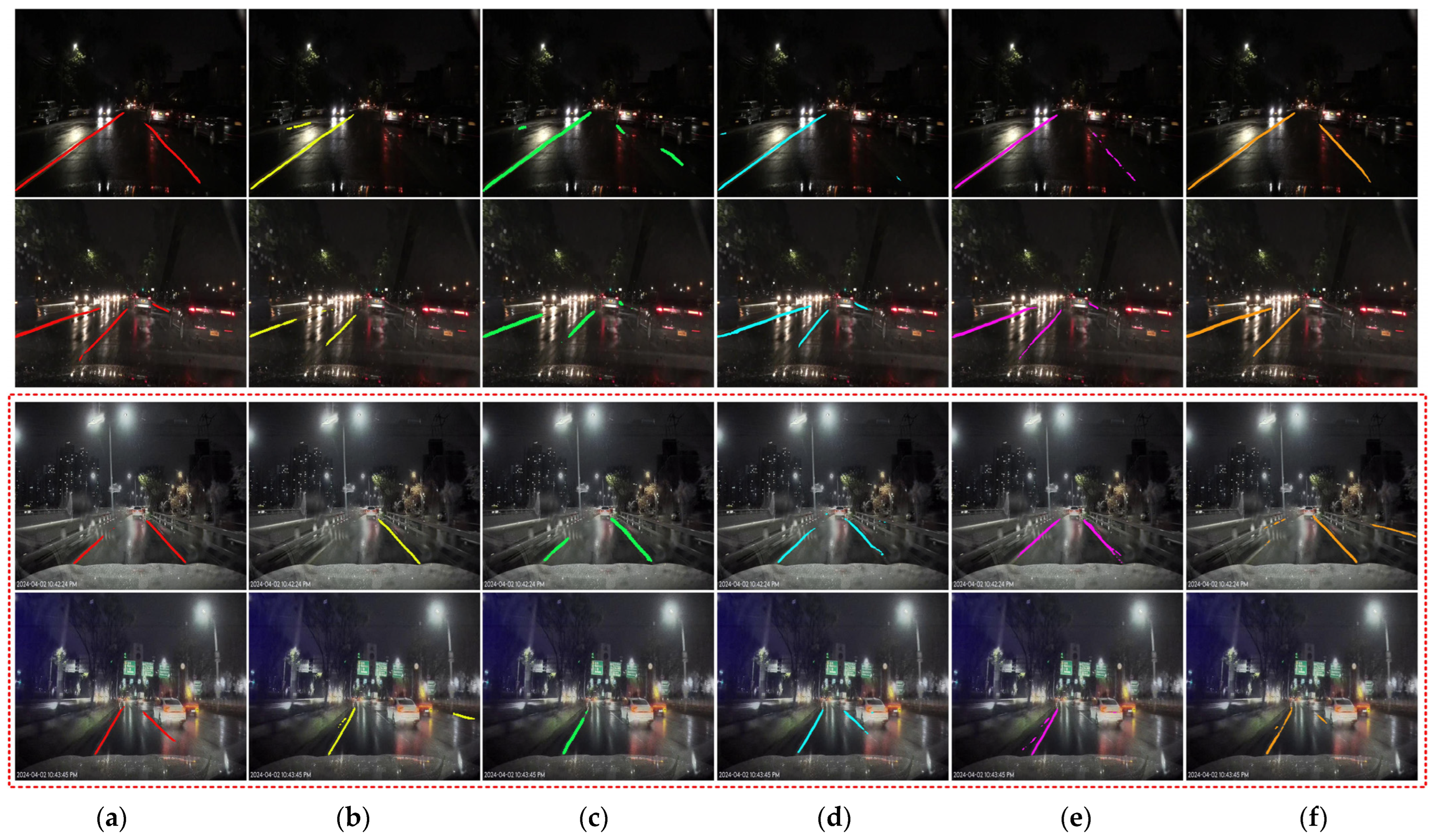
Figure 13.
The result of the evaluation in scenario 4 (the red dotted box represents the Lab. dataset): (a) proposed method (Case 1), (b) Case 2, (c) Case 3, (d) Case 4, (e) Case 5, and (f) Case 6.
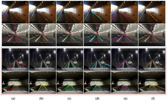
Figure 14.
The result of the evaluation in scenario 5 (the red dotted box represents the Lab. dataset): (a) proposed method (Case 1), (b) Case 2, (c) Case 3, (d) Case 4, (e) Case 5, and (f) Case 6.
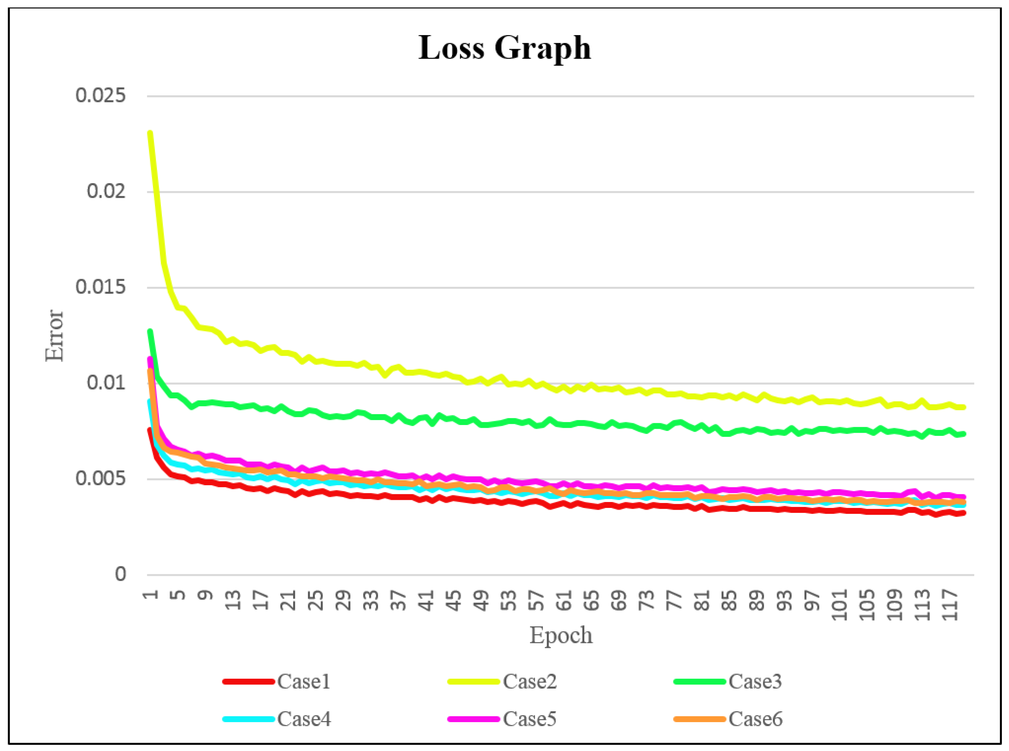
The loss for each case is represented in Figure 15. From the graph, it is evident that Case 1 exhibited the most stable decrease in loss. This result indicated that the 4-channel input was significantly more stable in terms of learning compared to the 3-channel input. This implies that providing additional information about the lanes during training ensured stable learning.
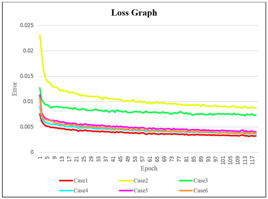
Figure 15.
Loss graph displaying evaluation.
4.4. Results of Performance Comparison Experiments
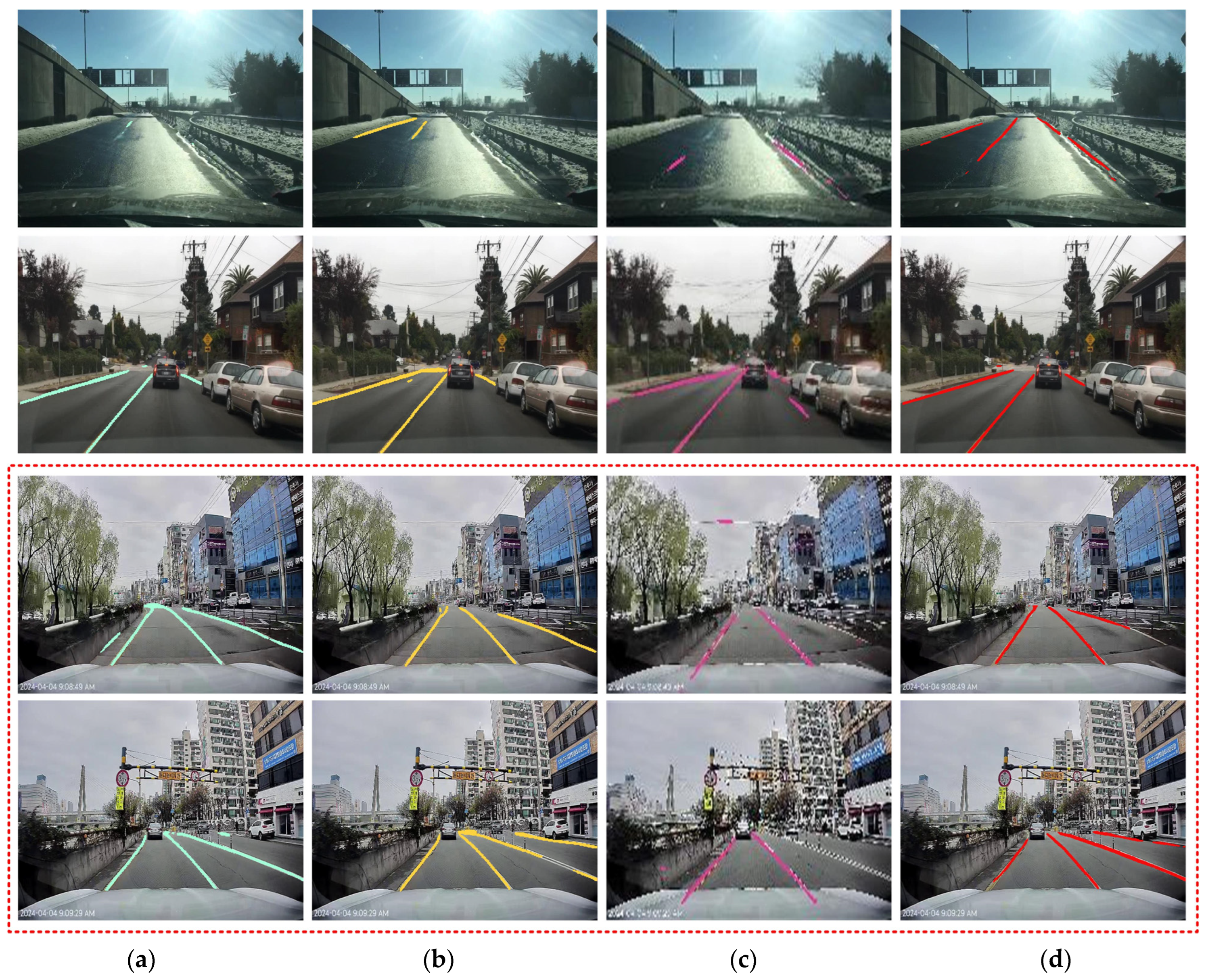
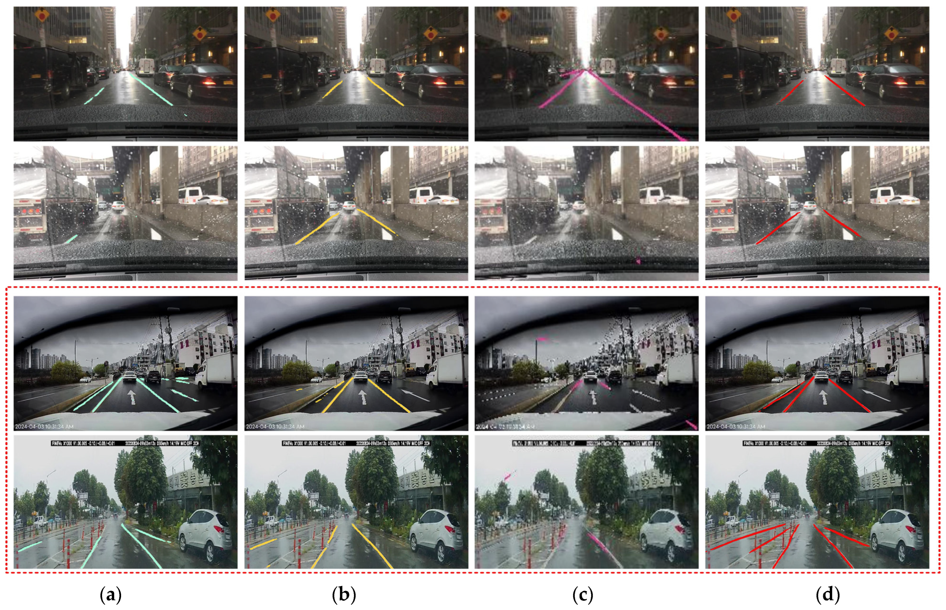
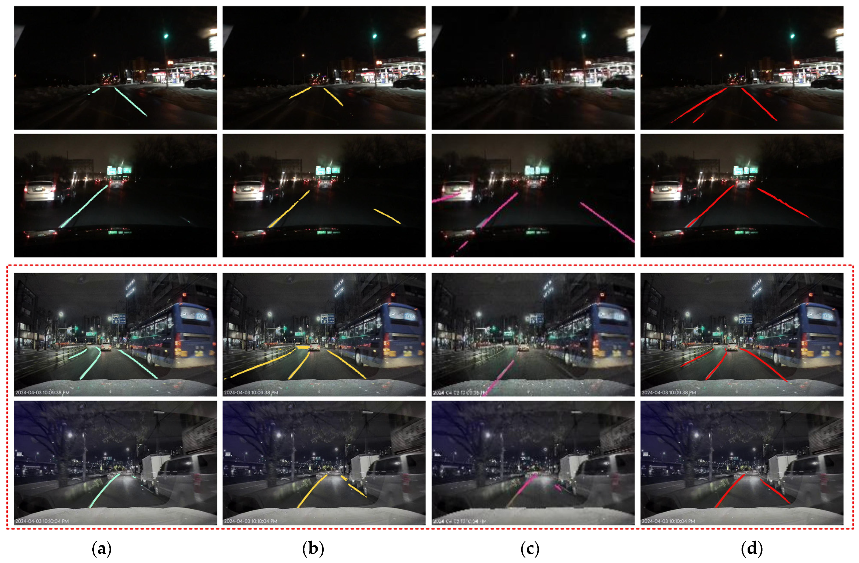
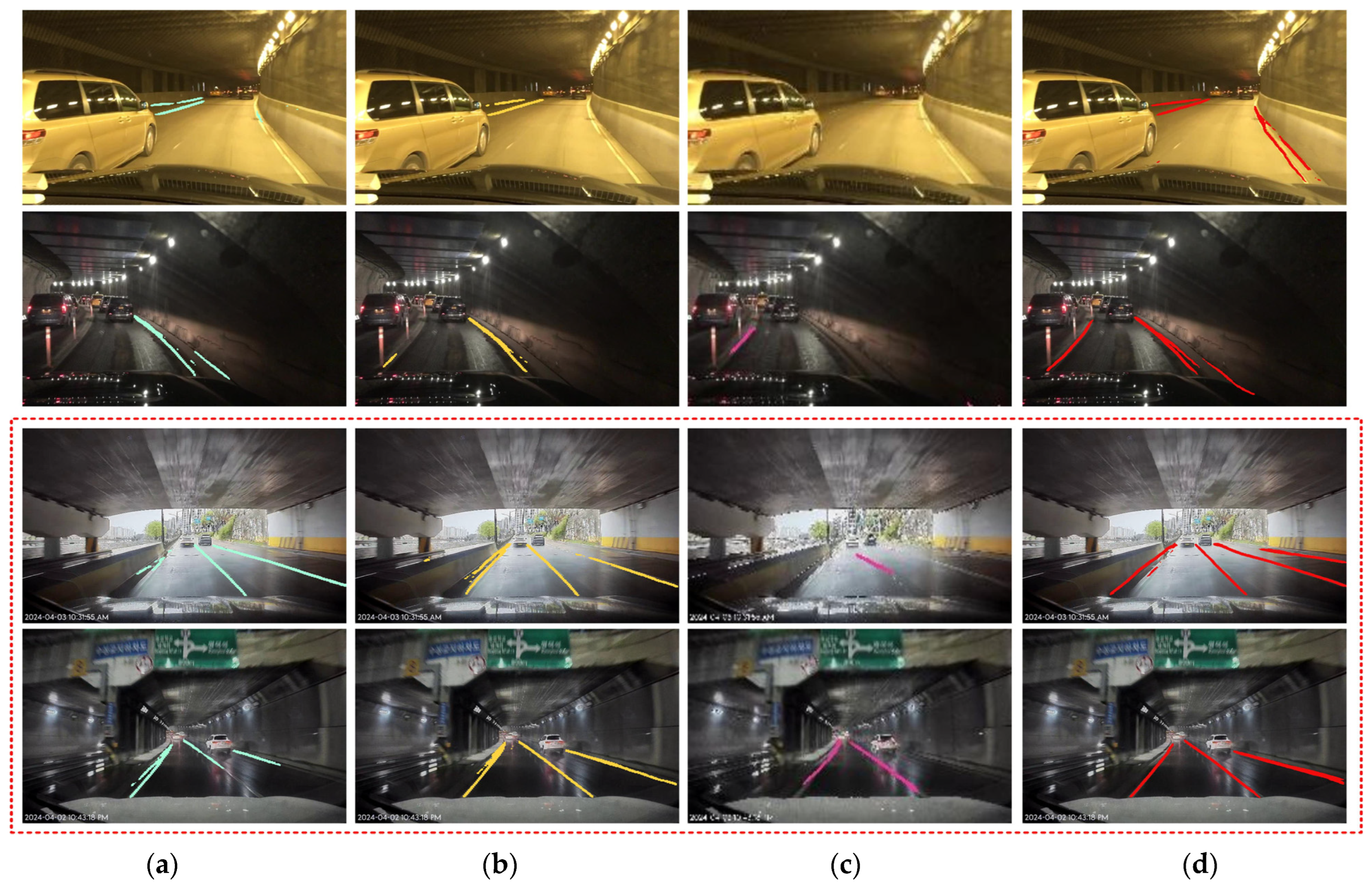
In this section, the superiority of the proposed method is demonstrated by comparing the results with those obtained using different approaches. All the experiments were conducted using the same set of 30,000 training data samples. The learning rate was set to 2 × , the batch size was 24, and the number of epochs was 120. Table 2 presents a comparison of the accuracies. U-Net [7], DSU-Net [29], ConvLSTM [28], and the proposed method were compared. It is evident that the detection rate of the proposed method was higher in both the left and right lane categories. For performance evaluation, comparison experiments were conducted in five scenarios, each comprising 100 images, to increase the reliability of the experiments. Table 2 and Figure 16, Figure 17, Figure 18, Figure 19 and Figure 20 depict the results of each case. Despite the deterioration in image quality due to the structural limitation of the U-Net ConvLSTM model, which outputs only at 256 × 128 resolution, lane detection can still be visually confirmed. Since there are environmental differences between day and night, the comparison was split accordingly. Lee at al. proposed a method that applies Depthwise separable convolution to the conventional U-Net architecture, significantly reducing parameters by nearly four times for real-time operation [29]. Similarly, our approach also employs Depthwise separable convolution to reduce parameters; however, to enhance detection rates, we increased the depth of the existing standard U-Net architecture. As a result, the parameters required for training increased nearly fourfold.
Table 2.
Comparison experiments with other algorithms.
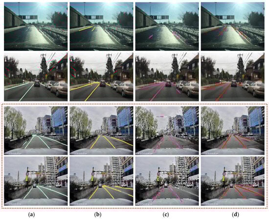
Figure 16.
The result of the comparison in scenario 1 (the red dotted box represents the Lab. dataset): (a) U-Net lane detection, (b) Depthwise separable U-Net, (c) U-Net ConvLSTM, and (d) proposed method.
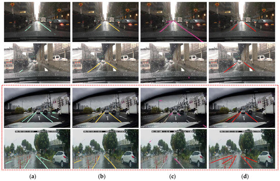
Figure 17.
The result of the comparison in scenario 2 (the red dotted box represents the Lab. dataset): (a) U-Net lane detection, (b) Depthwise separable U-Net, (c) U-Net ConvLSTM, and (d) proposed method.
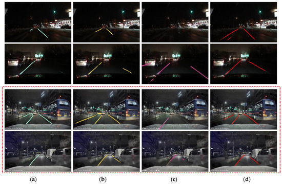
Figure 18.
The result of the comparison in scenario 3 (the red dotted box represents the Lab. dataset): (a) U-Net lane detection, (b) Depthwise separable U-Net, (c) U-Net ConvLSTM, and (d) proposed method.
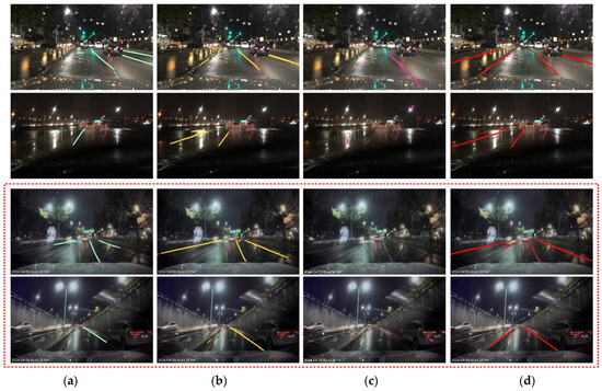
Figure 19.
The result of the comparison in scenario 4 (the red dotted box represents the Lab. dataset): (a) U-Net lane detection, (b) Depthwise separable U-Net, (c) U-Net ConvLSTM, and (d) proposed method.
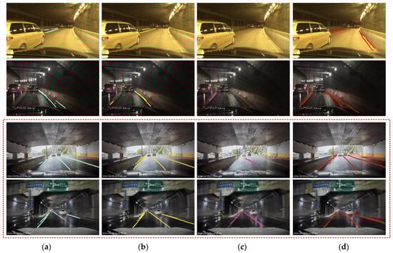
Figure 20.
The result of the comparison in scenario 5 (the red dotted box represents the Lab. dataset): (a) U-Net lane detection, (b) Depthwise separable U-Net, (c) U-Net ConvLSTM, and (d) proposed method.
5. Conclusions
In this paper, a learning approach for stable lane detection in various environments was proposed. First, the training dataset was refined, where the RGB color space was transformed into the Lab color space and only the L channel information was used to prevent color distortion. Situation-appropriate bilateral filters and MSR were applied to suppress noise and increase contrast, refining images captured in harsh road environments for lane detection. Additionally, a method was proposed for enhancing efficiency in training by combining edge images passed through a directional edge filter (emphasizing lane information) as the fourth channel. Directional edge filters were employed to emphasize the left and right lanes in the edge image. The refined training dataset was referred to as four-channel input data. To train with the four-channel input data, the structure of U-Net was modified, with layers added for deeper learning. In addition, the input and output of the added layers were disregarded to prevent overfitting. Furthermore, the Depthwise separable convolutions technique was applied to reduce the number of parameters, providing overall lightening of the model. Finally, to prevent unnecessary areas outside the lane from affecting the loss calculation, the loss was only computed in regions where lanes potentially existed. Adjusting the impact of loss through a parameter tuner accelerated the learning. The proposed learning approach demonstrated more stable training and better detection rates compared to other methods, as evidenced by loss graphs, comparison tables, and result images. However, as this method was only evaluated on a single structure based on U-Net, it will be necessary to evaluate this new learning approach on a wider range of modules. Furthermore, our proposed method cannot operate in real-time, due to the increased number of parameters for higher detection rates. In future research, we will explore ways to reduce the parameter count while maintaining high detection rates to enable real-time operation. Additionally, our goal is to continue researching by experimenting with real-time lane detection using embedded ASIC boards. Future research should consider both lane detection and other vehicle recognition tasks, along with a consideration of real-time operation by embedding systems into vehicles.
Author Contributions
Conceptualization, S.-H.L. (Sung-Hak Lee); methodology, S.-H.L. (Seung-Hwan Lee) and S.-H.L. (Sung-Hak Lee); software, S.-H.L. (Seung-Hwan Lee); validation, S.-H.L. (Seung-Hwan Lee) and S.-H.L. (Sung-Hak Lee); formal analysis, S.-H.L. (Seung-Hwan Lee) and S.-H.L. (Sung-Hak Lee); investigation, S.-H.L. (Seung-Hwan Lee) and S.-H.L. (Sung-Hak Lee); resources, S.-H.L. (Seung-Hwan Lee) and S.-H.L. (Sung-Hak Lee); data curation, S.-H.L. (Seung-Hwan Lee) and S.-H.L. (Sung-Hak Lee); writing—original draft preparation, S.-H.L. (Seung-Hwan Lee); writing—review and editing, S.-H.L. (Sung-Hak Lee); visualization, S.-H.L. (Seung-Hwan Lee); supervision, S.-H.L. (Sung-Hak Lee); project administration, S.-H.L. (Sung-Hak Lee); funding acquisition, S.-H.L. (Sung-Hak Lee). All authors have read and agreed to the published version of the manuscript.
Funding
This research was supported by the Basic Science Research Program through the National Research Foundation of Korea (NRF), funded by the Ministry of Education, Korea (NRF-2021R1I1A3049604, 50%) and supported by Innovative Human Resource Development for Local Intellectualization program through the Institute of Information & Communications Technology Planning & Evaluation (IITP) grant funded by the Korea government (MSIT) (IITP-2024-RS-2022-00156389, 50%).
Data Availability Statement
The data presented in this study are openly available in https://bair.berkeley.edu/blog/2018/05/30/bdd/ (accessed on 20 March 2024) and the data presented in this study are available on request from the corresponding author.
Conflicts of Interest
The authors declare no conflict of interest.
References
- Iandola, F.N.; Han, S.; Moskewicz, M.W.; Ashraf, K.; Dally, W.J.; Keutzer, K. SqueezeNet: AlexNet-Level Accuracy with 50x Fewer Parameters and <0.5MB Model Size. arXiv 2016, arXiv:1602.07360. [Google Scholar]
- Li, J.; Mei, X.; Prokhorov, D.; Tao, D. Deep Neural Network for Structural Prediction and Lane Detection in Traffic Scene. IEEE Trans. Neural Netw. Learn. Syst. 2017, 28, 690–703. [Google Scholar] [CrossRef] [PubMed]
- Tian, Y.; Zhang, Y.; Zhang, H. Recent Advances in Stochastic Gradient Descent in Deep Learning. Mathematics 2023, 11, 682. [Google Scholar] [CrossRef]
- Oros, G.I.; Dzitac, S. Applications of Subordination Chains and Fractional Integral in Fuzzy Differential Subordinations. Mathematics 2022, 10, 1690. [Google Scholar] [CrossRef]
- Zhou, Y.; Xu, R.; Hu, X.; Ye, Q. A Robust Lane Detection and Tracking Method Based on Computer Vision. Meas. Sci. Technol. 2006, 17, 736–745. [Google Scholar] [CrossRef]
- Tang, J.; Li, S.; Liu, P. A Review of Lane Detection Methods Based on Deep Learning. Pattern Recognit. 2021, 111, 107623. [Google Scholar] [CrossRef]
- Ronneberger, O.; Fischer, P.; Brox, T. U-Net: Convolutional Networks for Biomedical Image Segmentation. In Proceedings of the Medical Image Computing and Computer-Assisted Intervention—MICCAI 2015, Munich, Germany, 5–9 October 2015; Navab, N., Hornegger, J., Wells, W.M., Frangi, A.F., Eds.; Springer International Publishing: Cham, Switzerland, 2015; pp. 234–241. [Google Scholar]
- Das, S.; Pratihar, S.; Pradhan, B.; Jhaveri, R.H.; Benedetto, F. IoT-Assisted Automatic Driver Drowsiness Detection through Facial Movement Analysis Using Deep Learning and a U-Net-Based Architecture. Information 2024, 15, 30. [Google Scholar] [CrossRef]
- Zhang, X.; Yang, W.; Tang, X.; Liu, J. A Fast Learning Method for Accurate and Robust Lane Detection Using Two-Stage Feature Extraction with YOLO V3. Sensors 2018, 18, 4308. [Google Scholar] [CrossRef] [PubMed]
- Ghafoorian, M.; Nugteren, C.; Baka, N.; Booij, O.; Hofmann, M. EL-GAN: Embedding Loss Driven Generative Adversarial Networks for Lane Detection. In Lecture Notes in Computer Science (Including Subseries Lecture Notes in Artificial Intelligence and Lecture Notes in Bioinformatics); Spring: Berlin/Heidelberg, Germany, 2019; Volume 11129, pp. 256–272. [Google Scholar] [CrossRef]
- Kenue, S.K. Lanelok: Detection of Lane Boundaries and Vehicle Tracking Using Image-Processing Techniques-Part II: Template Matching Algorithms. In Proceedings of the Mobile Robots IV, Philadelphia, PA, USA, 6–7 November 1989; Chun, W.H., Wolfe, W.J., Eds.; SPIE: Bellingham, WA, USA, 1990; Volume 1195, pp. 234–245. [Google Scholar]
- Goldbeck, J.; Huertgen, B. Lane Detection and Tracking by Video Sensors. In Proceedings of the 199 IEEE/IEEJ/JSAI International Conference on Intelligent Transportation Systems, Tokyo, Japan, 5–8 October 1999; pp. 74–79. [Google Scholar] [CrossRef]
- Illingworth, J.; Kittler, J. A Survey of the Hough Transform. Comput. Vis. Graph. Image Process. 1988, 44, 87–116. [Google Scholar] [CrossRef]
- Ding, Y.; Xu, Z.; Zhang, Y.; Sun, K. Fast Lane Detection Based on Bird’s Eye View and Improved Random Sample Consensus Algorithm. Multimed. Tools Appl. 2017, 76, 22979–22998. [Google Scholar] [CrossRef]
- Duong, T.T.; Pham, C.C.; Tran, T.H.P.; Nguyen, T.P.; Jeon, J.W. Near Real-Time Ego-Lane Detection in Highway and Urban Streets. In Proceedings of the 2016 IEEE International Conference on Consumer Electronics-Asia (ICCE-Asia), Seoul, Republic of Korea, 26–28 October 2016; pp. 1–4. [Google Scholar] [CrossRef]
- Wang, Y.; Shen, D.; Teoh, E. Lane Detection Using Catmull-Rom Spline. In Proceedings of the IEEE International Conference on Intelligent Vehicles, Stuttgart, Germany, 28–30 October 1998; pp. 51–57. [Google Scholar]
- Wang, Y.; Teoh, E.K.; Shen, D. Lane Detection and Tracking Using B-Snake. Image Vis. Comput. 2004, 22, 269–280. [Google Scholar] [CrossRef]
- Jung, C.R.; Kelber, C.R. Lane Following and Lane Departure Using a Linear-Parabolic Model. Image Vis. Comput. 2005, 23, 1192–1202. [Google Scholar] [CrossRef]
- Srivastava, S.; Singal, R.; Lumba, M. Efficient Lane Detection Algorithm Using Different Filtering Techniques. Int. J. Comput. Appl. 2014, 88, 6–11. [Google Scholar] [CrossRef]
- Wang, J.; Wu, Y.; Liang, Z.; Xi, Y. Lane Detection Based on Random Hough Transform on Region of Interesting. In Proceedings of the 2010 IEEE International Conference on Information and Automation, Harbin, China, 20–23 June 2010; pp. 1735–1740. [Google Scholar] [CrossRef]
- Javeed, M.A.; Ghaffar, M.A.; Ashraf, M.A.; Zubair, N.; Metwally, A.S.M.; Tag-Eldin, E.M.; Bocchetta, P.; Javed, M.S.; Jiang, X. Lane Line Detection and Object Scene Segmentation Using Otsu Thresholding and the Fast Hough Transform for Intelligent Vehicles in Complex Road Conditions. Electronics 2023, 12, 1079. [Google Scholar] [CrossRef]
- Son, Y.; Lee, E.S.; Kum, D. Robust Multi-Lane Detection and Tracking Using Adaptive Threshold and Lane Classification. Mach. Vis. Appl. 2019, 30, 111–124. [Google Scholar] [CrossRef]
- Lee, S.H.; Kwon, H.J.; Lee, S.H. Enhancing Lane-Tracking Performance in Challenging Driving Environments through Parameter Optimization and a Restriction System. Appl. Sci. 2023, 13, 9313. [Google Scholar] [CrossRef]
- Phueakjeen, W.; Jindapetch, N.; Kuburat, L.; Suvanvorn, N. A Study of the Edge Detection for Road Lane. In Proceedings of the 8th Electrical Engineering/Electronics, Computer, Telecommunications and Information Technology (ECTI) Association of Thailand—Conference 2011, Khon Kaen, Thailand, 17–19 May 2011; pp. 995–998. [Google Scholar] [CrossRef]
- Guo, J.; Wei, Z.; Miao, D. Lane Detection Method Based on Improved RANSAC Algorithm. In Proceedings of the 2015 IEEE Twelfth International Symposium on Autonomous Decentralized Systems, Taichung, Taiwan, 25–27 March 2015; pp. 285–288. [Google Scholar] [CrossRef]
- Borkar, A.; Hayes, M.; Smith, M.T. Robust Lane Detection and Tracking with Ransac and Kalman Filter. In Proceedings of the 16th IEEE International Conference on Image Processing (ICIP), Cairo, Egypt, 7–10 November 2009; pp. 3261–3264. [Google Scholar] [CrossRef]
- Tran, L.A.; Le, M.H. Robust U-Net-Based Road Lane Markings Detection for Autonomous Driving. In Proceedings of the 2019 International Conference on System Science and Engineering (ICSSE), Dong Hoi, Vietnam, 20–21 July 2019; pp. 62–66. [Google Scholar] [CrossRef]
- Zou, Q.; Jiang, H.; Dai, Q.; Yue, Y.; Chen, L.; Wang, Q. Robust Lane Detection from Continuous Driving Scenes Using Deep Neural Networks. IEEE Trans. Veh. Technol. 2020, 69, 41–54. [Google Scholar] [CrossRef]
- Lee, D.H.; Liu, J.L. End-to-End Deep Learning of Lane Detection and Path Prediction for Real-Time Autonomous Driving. Signal Image Video Process. 2023, 17, 199–205. [Google Scholar] [CrossRef]
- Feng, J.; Wu, X.; Zhang, Y. Lane Detection Base on Deep Learning. In Proceedings of the 2018 11th International Symposium on Computational Intelligence and Design, Hangzhou, China, 8–9 December 2018; Volume 1, pp. 315–318. [Google Scholar] [CrossRef]
- Lyu, Y.; Bai, L.; Huang, X. Road Segmentation Using CNN and Distributed LSTM. In Proceedings of the 2019 IEEE International Symposium on Circuits and Systems, Sapporo, Japan, 26–29 May 2019. [Google Scholar] [CrossRef]
- Li, L.; Xu, M.; Wang, X.; Jiang, L.; Liu, H. Attention Based Glaucoma Detection: A Large-Scale Database and CNN Model. In Proceedings of the 2019 IEEE/CVF Conference on Computer Vision and Pattern Recognition, Long Beach, CA, USA, 15–20 June 2019; pp. 10563–10572. [Google Scholar] [CrossRef]
- Li, J.; Lin, D.; Wang, Y.; Xu, G.; Zhang, Y.; Ding, C.; Zhou, Y. Deep Discriminative Representation Learning with Attention Map for Scene Classification. Remote Sens. 2020, 12, 1366. [Google Scholar] [CrossRef]
- Zhang, H.; Goodfellow, I.; Metaxas, D.; Odena, A. Self-Attention Generative Adversarial Networks. In Proceedings of the Proceedings of the 36th International Conference on Machine Learning, Long Beach, CA, USA, 9–15 June 2019; Chaudhuri, K., Salakhutdinov, R., Eds.; PMLR: New York, NY, USA, 2019; Volume 97, pp. 7354–7363. [Google Scholar]
- Chollet, F. Xception: Deep Learning With Depthwise Separable Convolutions. In Proceedings of the IEEE Conference on Computer Vision and Pattern Recognition (CVPR), Honolulu, HI, USA, 21–26 July 2017. [Google Scholar]

Disclaimer/Publisher’s Note: The statements, opinions and data contained in all publications are solely those of the individual author(s) and contributor(s) and not of MDPI and/or the editor(s). MDPI and/or the editor(s) disclaim responsibility for any injury to people or property resulting from any ideas, methods, instructions or products referred to in the content. |
© 2024 by the authors. Licensee MDPI, Basel, Switzerland. This article is an open access article distributed under the terms and conditions of the Creative Commons Attribution (CC BY) license (https://creativecommons.org/licenses/by/4.0/).