

Fixed/Preassigned-Time Synchronization of Fuzzy Memristive Fully Quaternion-Valued Neural Networks Based on Event-Triggered Control


Abstract
1. Introduction
- (1)
- Building on the foundational insights of established methods like the lexicographic order method and the metric function method [40,41,42], this paper embarks on a novel journey within the realm of quaternion analysis by redefining fuzzy rules. It further fortifies this innovation by rigorously analyzing and validating the accuracy and efficacy of the lemmas tied to the fuzzy rules, thereby setting a new benchmark in theoretical exploration.
- (2)
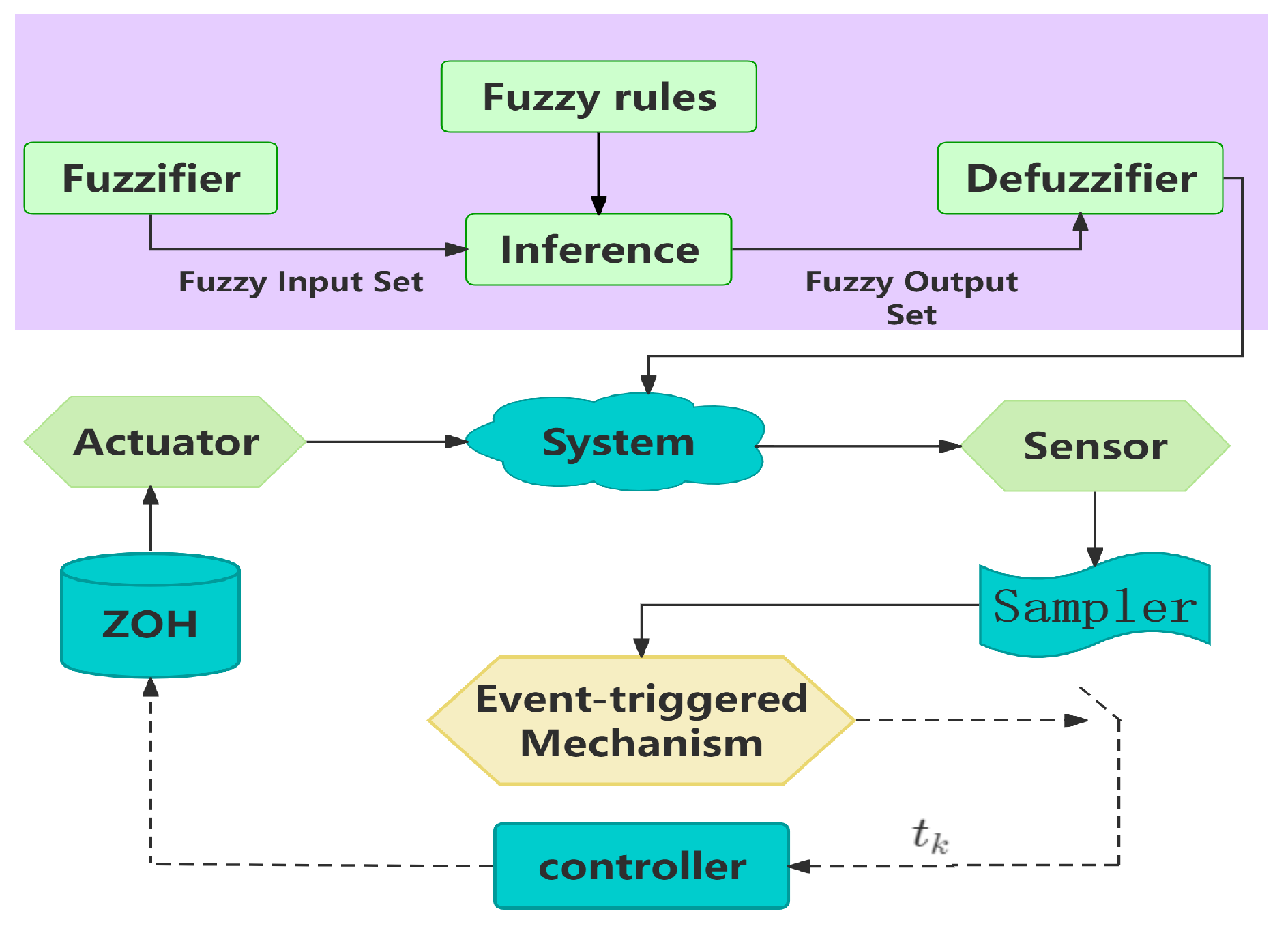
- Moving beyond traditional static event-triggering control mechanisms [43,44] with an eye towards enhancing communication efficiency, this paper introduces an innovative approach through the formulation of quaternion-valued dynamic event-triggering control strategies devoid of linear components. This strategic framework is designed to guarantee both FITS and PETS within the context of QVFMNNs. Additionally, the paper adeptly eliminates the potential for Zeno phenomena within the system by employing a methodical application of the proof by contradiction.
- (3)
- Different from the conventional separation technique, the FITS and PETS of QVFMNN are discussed through a direct analytical approach. Consequently, several flexible criteria are established for achieving FITS and PETS of QVFMNN and the upper bound of the setting time is provided explicitly.
2. Model Description and Preliminaries
3. Main Results
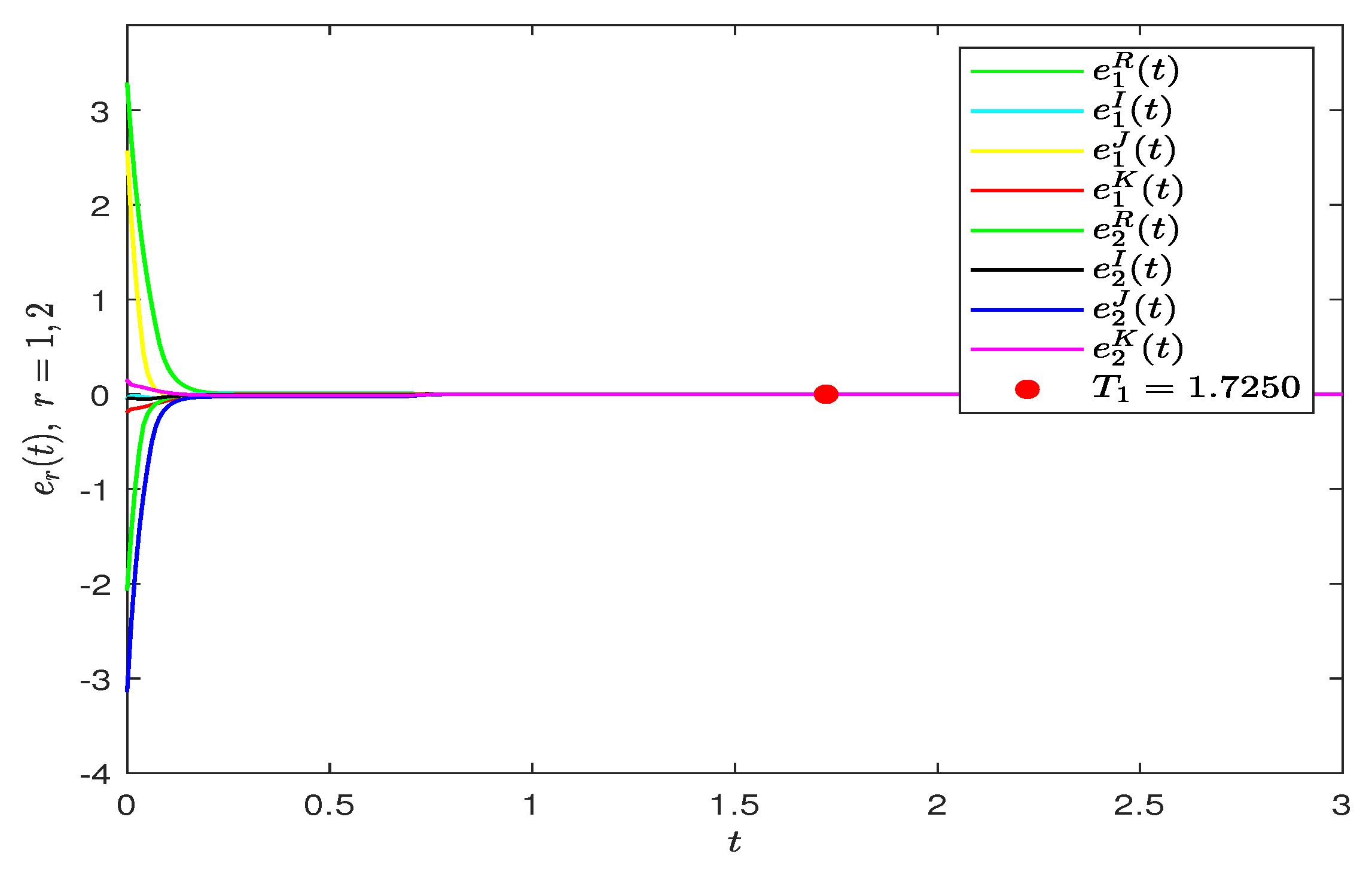
3.1. FITS
- (1)
- If , the FITS of QVFMNNs (1) and (3) can be realized and the ST is estimated by
- (2)
- If then for in which
- (3)
- If and then for in which
- (1)
- When , ,
- (2)
- When , ,
- (3)
- When , ,
- (4)
- When , ,
- (1)
- If , the FITS of systems (14) and (15) can be realized and the ST is estimated by
- (2)
- If then for where
- (3)
- If and then for where
- (1)
- If , the FITS of systems (18) and (19) can be realized and the ST is estimated by
- (2)
- If then for where
- (3)
- If and then for where
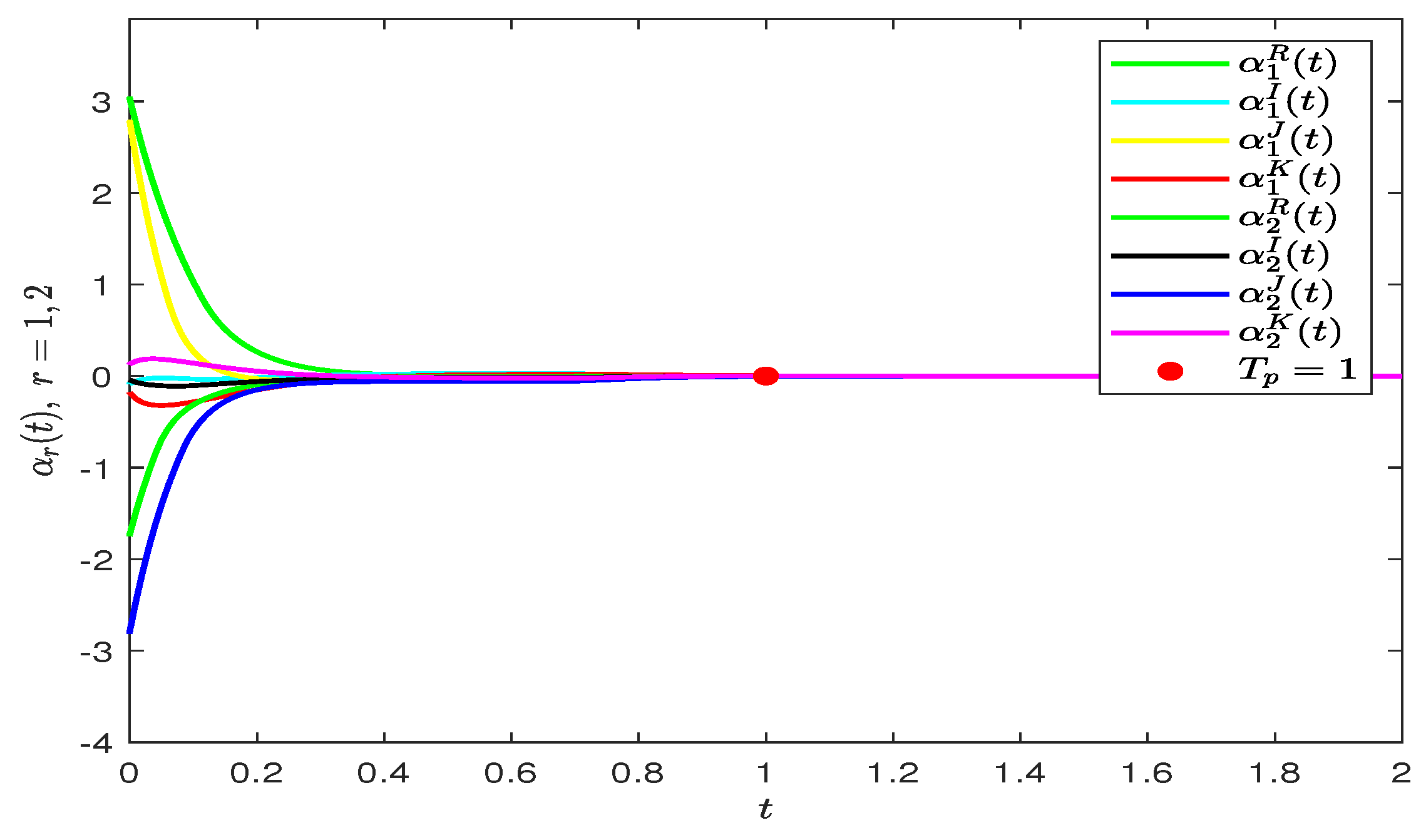
3.2. PETS
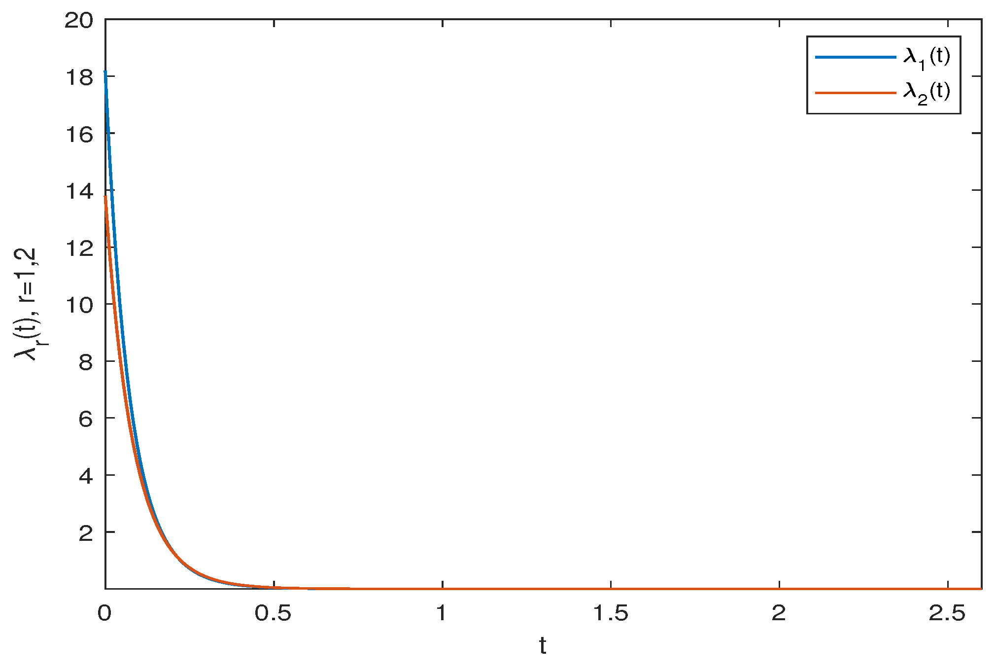
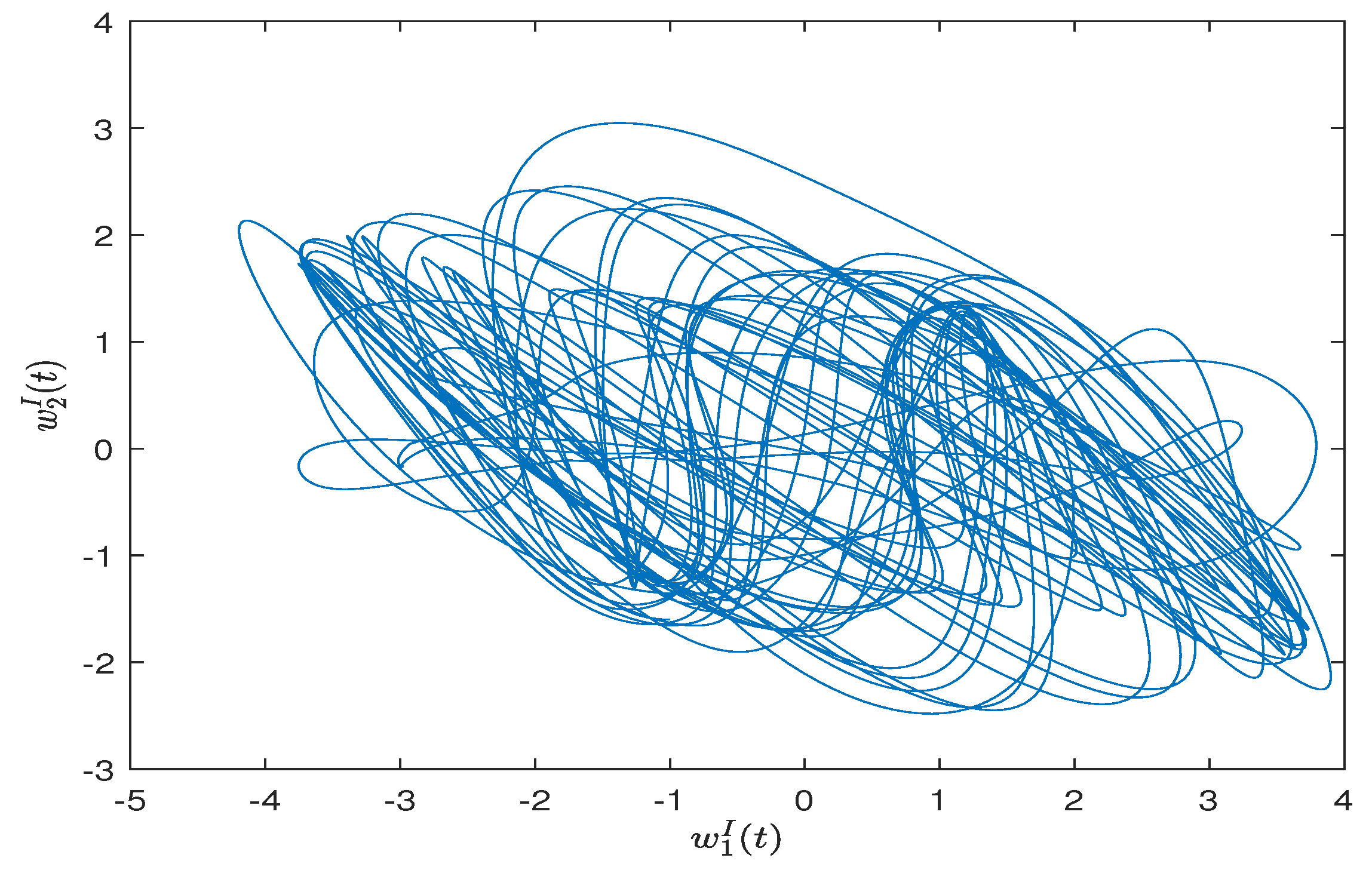
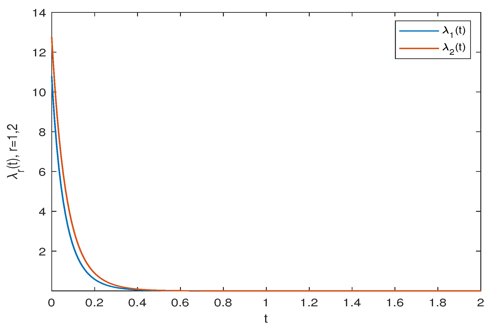
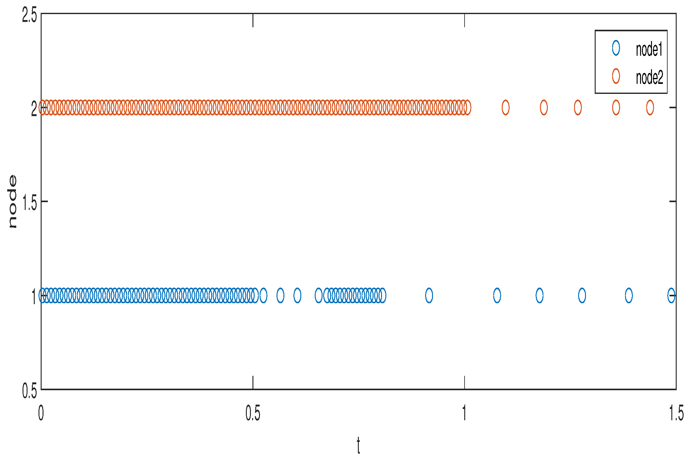
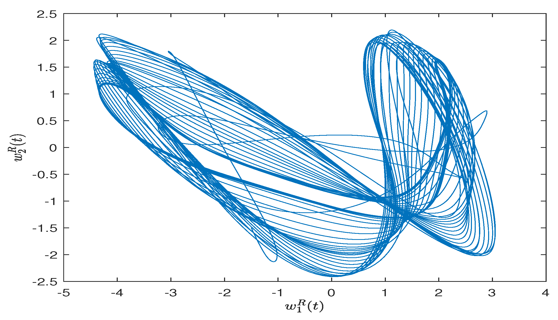
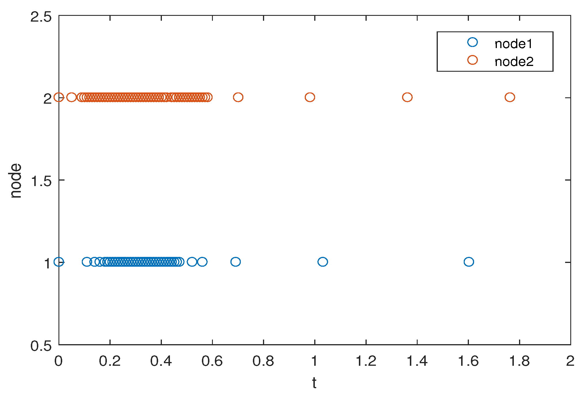
4. Numerical Simulations
5. Conclusions
Author Contributions
Funding
Data Availability Statement
Conflicts of Interest
Abbreviations
| The quaternion set | |
| The n-dimensional real number vector set | |
| The n-dimensional quaternion number vector set | |
| for any |
| The left limit of discontinuous function | |
| at point | |
| The right limit of discontinuous function | |
| at point | |
| The minimum of | |
| The maximum of | |
| , | |
References
- Liu, F.; Meng, W.; Lu, R. Anti-synchronization of discrete-time fuzzy memristive neural networks via impulse sampled-data communication. IEEE Trans. Cybern. 2023, 53, 4122–4133. [Google Scholar] [CrossRef] [PubMed]
- Wei, H.; Li, R. Exponential synchronization control of reaction-diffusion fuzzy memristive neural networks: Hardy-Poincare inequality. IEEE Trans. Neural Netw. Learn. Syst. 2023; online ahead of print. [Google Scholar] [CrossRef]
- Gong, S.; Guo, Z.; Wen, S. Finite-time synchronization of T-S fuzzy memristive neural networks with time delay. Fuzzy Sets Syst. 2022, 459, 67–81. [Google Scholar] [CrossRef]
- Wang, L.; Li, H.; Hu, C.; Hu, J.; Wang, Q. Synchronization and settling-time estimation of fuzzy memristive neural networks with time-varying delays: Fixed-time and preassigned-time control. Fuzzy Sets Syst. 2023, 470, 108654. [Google Scholar] [CrossRef]
- Davila-Meza, E.; Bayro-Corrochano, E. Quaternion and split quaternion neural networks for low-light color image enhancement. IEEE Access 2023, 11, 108257–108280. [Google Scholar] [CrossRef]
- Frants, V.; Agaian, S.; Panetta, K. QSAM-Net: Rain streak removal by quaternion neural network with self-attention module. IEEE Trans. Multimed. 2023, 26, 789–798. [Google Scholar] [CrossRef]
- Ni, H.; Xie, S.; Xu, P.; Fang, X.; Sun, W.; Fang, R. QMGR-Net: Quaternion multi-graph reasoning network for 3D hand pose estimation. Int. J. Mach. Learn. Cybern. 2023, 14, 4029–4045. [Google Scholar] [CrossRef]
- Shi, Y.; Chen, X.; Zhu, P. Dissipativity for a class of quaternion-valued memristor-based neutral-type neural networks with time-varying delays. Math. Methods Appl. Sci. 2023, 46, 18166–18194. [Google Scholar] [CrossRef]
- Aouiti, C.; Touati, F. Global dissipativity of quaternion-valued fuzzy cellular fractional-order neural networks with time delays. Neural Process. Lett. 2022, 55, 481–503. [Google Scholar] [CrossRef]
- Chen, Y.; Xue, Y.; Yang, X.; Zhang, X. A direct analysis method to Lagrangian global exponential stability for quaternion memristive neural networks with mixed delays. Appl. Math. Comput. 2022, 439, 127633. [Google Scholar] [CrossRef]
- Liu, Y.; Zhang, D.; Lou, J.; Lu, J.; Cao, J. Stability analysis of quaternion-valued neural networks: Decomposition and direct approaches. IEEE Trans. Neural Netw. Learn. Syst. 2018, 29, 4201–4211. [Google Scholar] [CrossRef]
- Liu, Y.; Zheng, Y.; Lu, J.; Cao, J.; Rutkowski, L. Constrained quaternion-variable convex optimization: A quaternion-valued recurrent neural network approach. IEEE Trans. Neural Netw. Learn. Syst. 2020, 31, 1022–1035. [Google Scholar] [CrossRef]
- Peng, T.; Wu, Y.; Tu, Z.; Alofi, A.; Lu, J. Fixed-time and prescribed-time synchronization of quaternion-valued neural networks: A control strategy involving Lyapunov functions. Neural Netw. 2023, 160, 108–121. [Google Scholar] [CrossRef] [PubMed]
- Shang, W.; Zhang, W.; Chen, D.; Cao, J. New criteria of finite time synchronization of fractional-order quaternion-valued neural networks with time delay. Appl. Math. Comput. 2022, 436, 127484. [Google Scholar] [CrossRef]
- Zhang, L.; Wei, R.; Cao, J.; Ding, X. Synchronization control of quaternion-valued inertial memristor-based neural networks via adaptive method. Math. Methods Appl. Sci. 2024, 47, 581–599. [Google Scholar] [CrossRef]
- Zhang, T.; Jian, J. Quantized intermittent control tactics for exponential synchronization of quaternion-valued memristive delayed neural networks. ISA Trans. 2021, 126, 288–299. [Google Scholar] [CrossRef] [PubMed]
- Lin, D.; Chen, X.; Yu, G.; Li, Z.; Xia, Y. Global exponential synchronization via nonlinear feedback control for delayed inertial memristor-based quaternion-valued neural networks with impulses. Appl. Math. Comput. 2021, 401, 126093. [Google Scholar] [CrossRef]
- Aouiti, C.; Jallouli, H. New feedback control techniques of quaternion fuzzy neuralnetworks with time-varying delay. Int. J. Robust Nonlinear Control 2021, 31, 2783–2809. [Google Scholar] [CrossRef]
- Wang, P.; Li, X.; Wang, N.; Li, Y.; Shi, K.; Lu, J. Almost periodic synchronization of quaternion-valued fuzzy cellular neural networks with leakage delays. Fuzzy Sets Syst. 2021, 426, 46–65. [Google Scholar] [CrossRef]
- Narayanan, G.; Ali, M.; Alam, M.; Rajchakit, G.; Boonsatit, N.; Kumar, P.; Hammachukiattikul, P. Adaptive fuzzy feedback controller design for finite-time mittag-leffler synchronization of fractional-order quaternion-valued reaction-diffusion fuzzy molecular modeling of delayed neural networks. IEEE Access 2021, 9, 130862–130883. [Google Scholar] [CrossRef]
- Tang, Q.; Qu, S.; Zheng, W.; Du, X.; Tu, Z. New fixed-time stability criterion and fixed-time synchronization of neural networks via non-chattering control. Neural Comput. Appl. 2022, 35, 6029–6041. [Google Scholar] [CrossRef]
- Chouhan, S.; Kumar, U.; Das, S.; Cao, J. Fixed time synchronization of octonion valued neural networks with time varying delays. Eng. Appl. Artif. Intell. 2022, 118, 105684. [Google Scholar] [CrossRef]
- Wang, D.; Li, L. Fixed-time synchronization of delayed memristive neural networks with impulsive effects via novel fixed-time stability theorem. Neural Netw. 2023, 163, 75–85. [Google Scholar] [CrossRef] [PubMed]
- Jia, T.; Chen, X.; Zhao, F.; Cao, J.; Qiu, J. Adaptive fixed-time synchronization of stochastic memristor-based neural networks with discontinuous activations and mixed delays. J. Frankl. Inst. 2022, 360, 3364–3388. [Google Scholar] [CrossRef]
- Hu, C.; He, H.; Jiang, H. Fixed/Preassigned-time synchronization of complex networks via improving fixed-yime stability. IEEE Trans. Cybern. 2021, 51, 2882–2892. [Google Scholar] [CrossRef]
- Rezaie, A.; Mobayen, S.; Ghaemi, M.; Fekih, A.; Zhilenkov, A. Design of a fixed-time stabilizer for uncertain chaotic systems subject to external disturbances. Mathematics 2023, 15, 3273. [Google Scholar] [CrossRef]
- Yang, W.; Xiao, L.; Huang, J.; Yang, J. Fixed-time synchronization of neural networks based on quantized intermittent control for image protection. Mathematics 2021, 23, 3086. [Google Scholar] [CrossRef]
- Pang, L.; Hu, C.; Yu, J.; Jiang, H. Fixed-time synchronization for fuzzy-based impulsive complex networks. Mathematics 2022, 9, 1533. [Google Scholar] [CrossRef]
- Liu, H.; Cheng, J.; Cao, J.; Katib, I. Preassigned-time synchronization for complex-valued memristive neural networks with reaction-diffusion terms and Markov parameters. Neural Netw. 2023, 169, 520–531. [Google Scholar] [CrossRef] [PubMed]
- Zhou, X.; Cao, J.; Wang, X. Predefined-time synchronization of coupled neural networks with switching parameters and disturbed by Brownian motion. Neural Netw. 2023, 160, 97–107. [Google Scholar] [CrossRef]
- Yuan, J.; Zhang, C.; Chen, T. Command filtered adaptive neural network synchronization control of nonlinear stochastic systems with Lévy noise via event-triggered mechanism. IEEE Access 2021, 9, 146195–146202. [Google Scholar] [CrossRef]
- Yao, W.; Wang, C.; Sun, Y.; Gong, S.; Lin, H. Event-triggered control for robust exponential synchronization of inertial memristive neural networks under parameter disturbance. Neural Netw. 2023, 164, 67–80. [Google Scholar] [CrossRef] [PubMed]
- Bao, Y.; Zhang, Y.; Zhang, B. Fixed-time synchronization of coupled memristive neural networks via event-triggered control. Appl. Math. Comput. 2021, 411, 126542. [Google Scholar] [CrossRef]
- Zhu, S.; Bao, H. Event-triggered synchronization of coupled memristive neural networks. Appl. Math. Comput. 2022, 415, 126715. [Google Scholar] [CrossRef]
- Ge, C.; Liu, X.; Liu, Y.; Hua, C. Event-triggered exponential synchronization of the switched neural networks with frequent asynchronism. IEEE Trans. Neural Netw. Learn. Syst. 2024, 35, 1750–1760. [Google Scholar] [CrossRef] [PubMed]
- Guo, H.; Liu, J.; Ahn, C.; Wu, Y.; Li, W. Dynamic event-triggered impulsive control for stochastic nonlinear systems with extension in complex networks. IEEE Trans. Circuits Syst. I Regul. Pap. 2022, 69, 2167–2178. [Google Scholar] [CrossRef]
- Sun, J.; Wang, Y.; Wu, Y.; Zhou, Y.; Liu, J. Dynamic event-triggered control for fixed-time synchronization of Kuramoto-Oscillator networks with and without a pacemaker. Intell. Control Appl. 2023, 111, 10147–10162. [Google Scholar] [CrossRef]
- Ge, C.; Chang, C.; Liu, Y.; Hua, C. Dynamic event-triggered exponential synchronization for neural networks with random controller gain perturbations. Int. J. Control Autom. Syst. 2023, 21, 2927–2937. [Google Scholar] [CrossRef]
- Jia, S.; Hu, C.; Jiang, H. Fixed/Preassigned-time synchronization of fully quaternion-valued cohen–grossberg neural networks with generalized time delay. Mathematics 2023, 11, 4825. [Google Scholar] [CrossRef]
- Li, R.; Cao, J. Dissipativity and synchronization control of quaternion-valued fuzzy memristive neural networks: Lexicographical order method. Fuzzy Sets Syst. 2021, 443, 70–89. [Google Scholar] [CrossRef]
- Li, R.; Gao, X.; Cao, J. Quasi-state estimation and quasi-synchronization control of quaternion-valued fractional-order fuzzy memristive neural networks: Vector ordering approach. Appl. Math. Comput. 2019, 362, 124572. [Google Scholar] [CrossRef]
- Li, R.; Cao, J.; Li, N. Quasi-synchronization control of quaternion-valued fuzzy memristive neural networks. Fuzzy Sets Syst. 2023, 472, 108701. [Google Scholar] [CrossRef]
- Zhang, Z.; Wang, S.; Wang, X.; Wang, Z.; Lin, C. Event-triggered synchronization for delayed quaternion-valued inertial fuzzy neural networks via nonreduced order approach. IEEE Trans. Fuzzy Syst. 2023, 31, 3000–3014. [Google Scholar] [CrossRef]
- Wei, R.; Cao, J. Synchronization control of quaternion-valued memristive neural networks with and without event-triggered scheme. Cogn. Neurodyn. 2019, 13, 489–502. [Google Scholar] [CrossRef] [PubMed]
- Clarke, F. Optimization and Nonsmooth Analysis; Wiley: New York, NY, USA, 1983. [Google Scholar]
- Filippov, A. Differential Equations with Discontinuous Right-Hand Sides; Kluwer: Boston, MA, USA, 1988. [Google Scholar]
- Huang, L.; Guo, Z.; Wang, J. Theory and Applications of Differential Equations with Discontinuous Right-Hand Sides; Science Press: Beijing, China, 2011. [Google Scholar]
- Aubin, J.; Frankowska, H. Set-Valued Analysis; Birkhäuser: Boston, MA, USA, 1990. [Google Scholar]
- Wei, W.; Hu, C.; Yu, J.; Jiang, H. Fixed/preassigned-time synchronization of quaternion-valued neural networks involving delays and discontinuous activations: A direct approach. Acta Math. Sci. 2022, 43, 1439–1461. [Google Scholar] [CrossRef]


| Parameter Selection Steps in Theorem 1. |
|---|
| Step 1: the value of is calculated by using the parameters and . |
| Step 2: choose control parameters and in the controller (5) and (6). |
| Step 3: estimate the setting time . |
| Step 4: draw the simulation result of FITS. |
Disclaimer/Publisher’s Note: The statements, opinions and data contained in all publications are solely those of the individual author(s) and contributor(s) and not of MDPI and/or the editor(s). MDPI and/or the editor(s) disclaim responsibility for any injury to people or property resulting from any ideas, methods, instructions or products referred to in the content. |
© 2024 by the authors. Licensee MDPI, Basel, Switzerland. This article is an open access article distributed under the terms and conditions of the Creative Commons Attribution (CC BY) license (https://creativecommons.org/licenses/by/4.0/).
Share and Cite
Jia, S.; Hu, C.; Jiang, H. Fixed/Preassigned-Time Synchronization of Fuzzy Memristive Fully Quaternion-Valued Neural Networks Based on Event-Triggered Control. Mathematics 2024, 12, 1276. https://doi.org/10.3390/math12091276
Jia S, Hu C, Jiang H. Fixed/Preassigned-Time Synchronization of Fuzzy Memristive Fully Quaternion-Valued Neural Networks Based on Event-Triggered Control. Mathematics. 2024; 12(9):1276. https://doi.org/10.3390/math12091276
Chicago/Turabian StyleJia, Shichao, Cheng Hu, and Haijun Jiang. 2024. "Fixed/Preassigned-Time Synchronization of Fuzzy Memristive Fully Quaternion-Valued Neural Networks Based on Event-Triggered Control" Mathematics 12, no. 9: 1276. https://doi.org/10.3390/math12091276
APA StyleJia, S., Hu, C., & Jiang, H. (2024). Fixed/Preassigned-Time Synchronization of Fuzzy Memristive Fully Quaternion-Valued Neural Networks Based on Event-Triggered Control. Mathematics, 12(9), 1276. https://doi.org/10.3390/math12091276