A Weighted Skew-Logistic Distribution with Applications to Environmental Data

Abstract

Skewness and bimodality properties are frequently observed when analyzing environmental data such as wind speeds, precipitation levels, and ambient temperatures. As an alternative to modeling data exhibiting these properties, we propose a flexible extension of the skew-logistic distribution. The proposal corresponds to a weighted version of the skewed logistic distribution, defined by a parametric weight function that allows shapes with up to three modes for the resulting density. Parameter estimation via the maximum likelihood approach is discussed. Simulation experiments are carried out to evaluate the performance of the estimators. Applications to environmental data illustrating the utility of the proposal are presented.

1. Introduction

The skew-logistic distribution is a continuous probability distribution used in the modeling of skewed unimodal data. Considering a logistic baseline distribution, the skew-logistic distribution can be understood as a member of the skewed distributions class proposed by Azzalini [1]. Specifically, the random variable X follows a skew-logistic distribution if its probability density function (PDF) is given by

$$\begin{array}{ccc}\hfill f_X\left(x\right)& =& \frac{2e^{-x}}{{\left(1+e^{-x}\right)}^2\left(1+e^{-\lambda x}\right)},x\in \mathbb{R},\hfill \end{array}$$

(1)

where $\lambda \in \mathbb{R}$ is a skewness parameter. This is usually denoted as $X\sim \mathrm{SLOG}\left(\lambda \right)$.

The PDF in (1) is characterized by having a flared shape that can be symmetric or asymmetric, depending on $\lambda$. If $\lambda <0$, then a left-skewed PDF is achieved. If $\lambda >0$, then a right-skewed PDF is achieved. If $\lambda =0$, then the PDF is symmetric and reduces to the PDF of the classic logistic distribution.

The r-th moment of $X\sim \mathrm{SLOG}\left(\lambda \right)$ can be written as $\mathbb{E}\left(X^r\right)=2{\mathbb{I}}_r\left(\lambda \right)$, where

$$\begin{array}{ccc}\hfill {\mathbb{I}}_r& =& {\int }_0^1{\left[-\log \left(\frac{1-u}{u}\right)\right]}^r\frac{u^{\lambda }}{u^{\lambda }+{(1-u)}^{\lambda }}du,r=1,2,\dots \hfill \end{array}$$

(2)

The skew-logistic distribution is considered a natural alternative to generalized logistic distributions discussed in Johnson et al. [2]. A comprehensive description of the mathematical properties of the skew-logistic distribution can be found in Nadarajah [3] and Gupta and Kundu [4].

Although the skew-logistic distribution can perform appropriately in a wide variety of settings where the data exhibit unimodality, it performs poorly in the presence of multimodality; that is, when there are multiple modes or peaks in the empirical distribution. The presence of multimodality can be explained by different reasons, including the existence of multiple groups or sub-populations with unique characteristics, or the existence of latent variables that significantly influence the distribution of the population. In such cases, a mixture distribution is one of the first alternatives considered for modeling; however, its use involves dealing with the non-identifiability problem. An extensive discussion of the logistic mixture model can be found in Rost [5]. Details of the non-identifiability problem in mixture models can be consulted in Aitkin and Rubin [6] and McLachlan et al. [7].

Various methods to introduce new flexible probability distributions can be found in the statistical literature. There are many examples that we could mention, but the approaches proposed in Elal-Olivero [8], Gómez et al. [9], Venegas et al. [10] and Bolfarine et al. [11] are especially attractive when trying to propose a new bimodal distribution.

A very popular methodology in the literature is that of weighted distributions proposed by Fisher [12] and Rao [13]. Suppose that X is a random variable with probability function $f\left(x\right)$. The weighted random variable $X_w$ has PDF

$$\begin{array}{c}\hfill f_{X_w}\left(x\right)=\frac{w\left(x\right)f\left(x\right)}{{\mu }_w},\end{array}$$

(3)

where $w(·)$ is a nonnegative weight function and ${\mu }_w=\mathbb{E}\left[W\left(X\right)\right]<\infty$.

A particularly outstanding case of weighted distributions is obtained by considering $w\left(x\right)=x$, which defines a size-biased (or length-biased) distribution. Size-biased distributions arise naturally in applied fields, such as reliability and survival analysis, when individuals or mechanical units are sampled with unequal probability due to the design of the experiment or due to the existing unequal probability of detection.

In this paper, we propose a weighted version of the skew-logistic distribution that can present asymmetric shapes with up to three modes. The new distribution arises from Equation (3), considering that $f(·)$ is the PDF of the skew-logistic distribution and $w(·)$ is a parametric function that we will describe in Section 2. We provide evidence that the performance of the new distribution, being flexible both in skewness and in shapes involving bimodality, can outperform important distributions in the literature, even outperform the logistic mixture model.

The rest of this article is organized as follows. In Section 2, fundamental properties of the new distribution, such as the PDF, cumulative distribution function, raw moments, and Fisher’s skewness coefficient, are derived. In Section 3, parameter estimation via the maximum likelihood method is discussed. In Section 4, an application example that considers two environmental datasets illustrates the usefulness of the proposal. Finally, Section 5 reports some concluding remarks.

2. The New Distribution and Its Properties

This section proposes the new probability distribution and studies some of its fundamental properties, such as the PDF, the cumulative distribution function (CDF), and the raw moments. In addition, a detailed description of the PDF shapes is developed.

2.1. Weighted Skew-Logistic Distribution

The following proposition presents the PDF of the new distribution.

Proposition 1.

Let $X\sim \mathrm{SLOG}\left(\lambda \right)$ and $w(·)$ be a parametric function given by

$$w\left(x\right)=\frac{1}{1+\alpha {\kappa }_{\lambda }}\left[1+\alpha {\left(\frac{x-{\mu }_{\lambda }}{{\sigma }_{\lambda }}\right)}^4\right],x,\lambda \in \mathbb{R},\alpha >0,$$

where

$$\begin{array}{ccc}\hfill {\mu }_{\lambda }=\mathbb{E}\left(X\right)& =& 2{\mathbb{I}}_1,\hfill \\ \hfill {\sigma }_{\lambda }^2=\mathbb{V}ar\left(X\right)& =& 2\left({\mathbb{I}}_2-2{\mathbb{I}}_1^2\right),\hfill \\ \hfill {\kappa }_{\lambda }=\mathbb{K}\left(X\right)& =& \frac{{\mathbb{I}}_4-8{\mathbb{I}}_1{\mathbb{I}}_3+24{\mathbb{I}}_1^2{\mathbb{I}}_2-24{\mathbb{I}}_1^4}{2{\left({\mathbb{I}}_2-2{\mathbb{I}}_1^2\right)}^2},\hfill \end{array}$$

(4)

such that ${\mathbb{I}}_r\left(\lambda \right)$, with $r=1,2,3,4$, is as in Equation (2). Then, the PDF of the weighted random variable $X_w$ is

$$\begin{array}{c}\hfill f_{X_w}(x;\lambda ,\alpha )=\frac{2}{1+\alpha {\kappa }_{\lambda }}\left[1+\alpha {\left(\frac{x-{\mu }_{\lambda }}{{\sigma }_{\lambda }}\right)}^4\right]\frac{e^{-x}}{{(1+e^{-x})}^2(1+e^{-\lambda x})},\end{array}$$

(5)

where $x\in \mathbb{R}$, $\lambda \in \mathbb{R}$ and $\alpha >0$.

Proof. 

If $w\left(x\right)=\{1+\alpha {[(x-{\mu }_{\lambda })/{\sigma }_{\lambda }]}^4\}/(1+\alpha {\kappa }_{\lambda })$, the result in (5) is obtained directly by substituting (1) into (3).    □

Remark 1. 

1. 

Considering that ${\kappa }_{\lambda }=\mathbb{K}\left(X\right)>4$, see [3], we note that $w\left(x\right)=\frac{1}{1+\alpha {\kappa }_{\lambda }}[1+\alpha {\left(\frac{x-{\mu }_{\lambda }}{{\sigma }_{\lambda }}\right)}^4]$ is a positive function for all $\alpha >0$ and $x,\lambda \in \mathbb{R}$.

2. 

From Equation (5), considering $C_0=1/(1+\alpha {\kappa }_{\lambda })$, it is verified that

$$\begin{array}{ccc}\hfill {\int }_{-\infty }^{\infty }{f}_{X_w}(x;\lambda ,\alpha )dx& =& {\int }_{-\infty }^{\infty }{C}_0\left[1+\alpha {\left(\frac{x-{\mu }_{\lambda }}{{\sigma }_{\lambda }}\right)}^4\right]f_{X_w}(x;\lambda )dx\hfill \\ & =& C_0\left[{\int }_{-\infty }^{\infty }{f}_{X_w}(x;\lambda ,\alpha )dx+{\int }_{-\infty }^{\infty }\alpha {\left(\frac{x-{\mu }_{\lambda }}{{\sigma }_{\lambda }}\right)}^4{f}_{X_w}(x;\lambda ,\alpha )dx\right]\hfill \\ & =& C_0\left\{1+\alpha \mathbb{E}\left[{\left(\frac{X-{\mu }_{\lambda }}{{\sigma }_{\lambda }}\right)}^4\right]\right\}\hfill \\ & =& C_0(1+\alpha {\kappa }_{\lambda })\hfill \\ & =& 1.\hfill \end{array}$$

Definition 1.

Let $X_w$ be a random variable with PDF given in (5), then we say that $X_w$ follows a weighted skew-logistic distribution. We will denote this as $X_w\sim \mathrm{WSLOG}(\lambda ,\alpha )$.

Corollary 1.

If $X_w\sim \mathrm{WSLOG}(\lambda ,\alpha )$, then the random variable $Y=\mu +\sigma X_w$, with $\mu \in \mathbb{R}$ and $\sigma >0$, follows the weighted skew-logistic distribution with location parameter μ and scale parameter σ. The PDF of Y is given by

$$\begin{array}{ccc}\hfill f_Y(y;\mu ,\sigma ,\lambda ,\alpha )& =& \frac{2}{\sigma (1+\alpha {\kappa }_{\lambda })}\left[1+\alpha {\left(\frac{y-{\mu }_1^{\prime }}{{\sigma }_1}\right)}^4\right]\hfill \\ \hfill & & \times \frac{e^{-z}}{{(1+e^{-z})}^2(1+e^{-\lambda z})},\hfill \end{array}$$

(6)

where $y\in \mathbb{R}$, $z=\frac{y-\mu }{\sigma }$, $\lambda \in \mathbb{R}$, $\alpha >0$, ${\mu }_1^{\prime }=2\sigma {\mathbb{I}}_1+\mu$ and ${\sigma }_1^2=2{\sigma }^2({\mathbb{I}}_2-2{\mathbb{I}}_1^2)$, such that ${\mathbb{I}}_j$, $j=1,2$ is as in (2).

We denote this as $Y\sim \mathrm{WSLOG}(\mu ,\sigma ,\lambda ,\alpha )$.

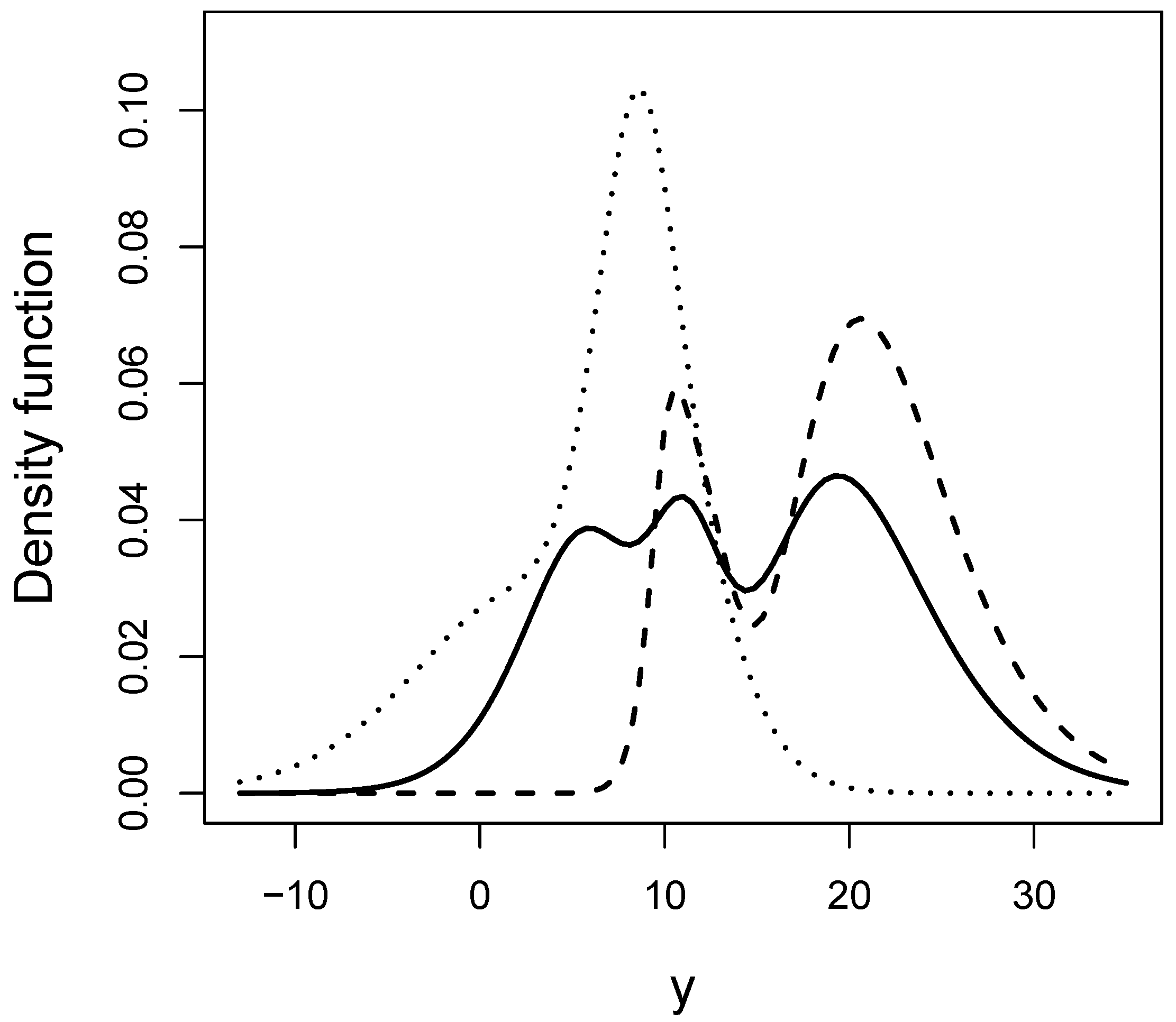
Figure 1 shows some PDF curves of the WSLOG distribution for different values of its parameters. In the figure, it can be seen that the WSLOG PDF can display shapes with up to three modes. These shapes will be described in more detail in Section 2.4.

2.2. Special Cases

The following proposition details the relationship between the WSLOG distribution with the logistic and SLOG distributions.

Proposition 2.

Let $X_w\sim \mathrm{WSLOG}(\lambda ,\alpha )$. Then,

1. 

${\displaystyle \underset{\alpha \to 0}{\lim }{f}_{X_w}(x,0,\alpha )=\frac{e^{-x}}{{(1+e^{-x})}^2}}$.

2. 

${\displaystyle \underset{\alpha \to 0}{\lim }{f}_{X_w}(x,\lambda ,\alpha )=\frac{2e^{-x}}{{\left(1+e^{-x}\right)}^2\left(1+e^{-\lambda x}\right)}}$.

3. 

${\displaystyle f_{X_w}(x,0,\alpha )=\left[1+\alpha {\left(\frac{x-{\mu }_0}{{\sigma }_0}\right)}^4\right]\frac{e^{-x}}{{(1+e^{-x})}^2}}$.

Proof. 

These results are the direct consequence of analyzing the limit case $\alpha \to 0$ of the WSLOG distribution, together with the special case $\lambda =0$ of the SLOG distribution.    □

Part (1) of Proposition 2 shows that WSLOG PDF tends to SLOG PDF as $\alpha \to 0$. Part (2) shows that the WSLOG PDF tends to the logistic PDF as $\alpha \to 0$ and $\lambda =0$. Part (3) presents a new PDF that can be understood as a bimodal extension of the logistic distribution. This new PDF is capable of displaying bimodal shapes while inheriting the symmetry feature of the logistic PDF.

2.3. Distribution Function and Related

In this section, we derive the cumulative distribution function (CDF) of the WSLOG distribution. This result will be used to compute goodness-of-fit tests in the application example of Section 4.

Proposition 3.

Let $Y\sim \mathrm{WSLOG}(\mu ,\sigma ,\lambda ,\alpha )$. Then, the CDF of Y is

$$\begin{array}{c}\hfill F_Y(y;\mu ,\sigma ,\lambda ,\alpha )=\frac{{\sigma }_1^4{F}_X(y;\mu ,\sigma ,\lambda )+2\alpha \mathbb{J}(y;\mu ,\sigma ,\lambda )}{{\sigma }_1^4(1+\alpha {\kappa }_{\lambda })},\end{array}$$

(7)

where $F_X(·;·,·,·)$ is the CDF of the location and scale version of the SLOG distribution, ${\sigma }_1$ y ${\kappa }_{\lambda }$ are as in Equation (6) and $\mathbb{J}(·;·,·,·)$ is given by

$$\begin{array}{c}\hfill \mathbb{J}(y;\mu ,\sigma ,\lambda )={\int }_{-\infty }^{\frac{y-\mu }{\sigma }}\frac{{(t\sigma +\mu -{\mu }_1)}^4}{(1+e^{-\lambda t})}\frac{e^{-t}}{{(1+e^{-t})}^2}dt.\end{array}$$

Proof. 

Denoting as $f_X(x;\mu ,\sigma ,\lambda )$ and $F_X(x;\mu ,\sigma ,\lambda )$ the PDF and the CDF of the SLOG distribution, respectively, from Equation (6), it is obtained that

$$\begin{array}{ccc}\hfill F_Y(y;\mu ,\sigma ,\lambda ,\alpha )& =& {\int }_{-\infty }^y{f}_Y(u;\mu ,\sigma ,\lambda ,\alpha )du\hfill \\ & =& \frac{1}{1+\alpha {\kappa }_{\lambda }}{\int }_{-\infty }^y\left[1+\alpha {\left(\frac{z-{\mu }_1}{{\sigma }_1}\right)}^4\right]f_X(u;\mu ,\sigma ,\lambda )du\hfill \\ & =& \frac{1}{{\sigma }_1^4(1+\alpha {\kappa }_{\lambda })}\left[{\sigma }_1^4{F}_X(y;\mu ,\sigma ,\lambda )+2\alpha {\int }_{-\infty }^{\frac{y-\mu }{\sigma }}\frac{{(t\sigma +\mu -{\mu }_1)}^4}{(1+e^{-\lambda t})}\frac{e^{-t}}{{(1+e^{-t})}^2}dt\right],\hfill \end{array}$$

and denoting the above integral as $\mathbb{J}(y;\mu ,\sigma ,\lambda )$, the result in (7) is obtained.    □

The following results are a direct consequence of the Proposition 3 and the Corollary 1.

Corollary 2.

If $Y\sim \mathrm{WSLOG}(\mu ,\sigma ,\lambda ,\alpha )$, the survival function (SF) of Y is

$$\begin{array}{ccc}\hfill S_Y(y;\mu ,\sigma ,\lambda ,\alpha )& =& 1-F_Y(y;\mu ,\sigma ,\lambda ,\alpha )\hfill \\ & =& 1-\frac{{\sigma }_1^4{F}_X(y;\mu ,\sigma ,\lambda )+2\alpha \mathbb{J}(y;\mu ,\sigma ,\lambda )}{{\sigma }_1^4(1+\alpha {\kappa }_{\lambda })}.\hfill \end{array}$$

Corollary 3.

If $Y\sim \mathrm{WSLOG}(\mu ,\sigma ,\lambda ,\alpha )$, the hazard rate function (HRF) of Y is

$$\begin{array}{ccc}\hfill h_Y(y;\mu ,\sigma ,\lambda ,\alpha )& =& \frac{f_Y(y;\mu ,\sigma ,\alpha ,\lambda )}{1-F_Y(y;\mu ,\sigma ,\lambda ,\alpha )}\hfill \\ & =& \frac{[{\sigma }_1^4+\alpha {(y-{\mu }_1)}^4]f_X(y;\mu ,\sigma ,\lambda )}{{\sigma }_1^4{F}_X(y;\mu ,\sigma ,\lambda )+2\alpha \mathbb{J}(y;\mu ,\sigma ,\lambda )}.\hfill \end{array}$$

Figure 2 presents some curves for the HRF of the WSLOG distribution for different parameter values. In the figure, it is possible to see that this function can present a roller coaster shape (increasing–decreasing–increasing).

2.4. Shapes

In order to provide more details regarding the shapes of the WSLOG distribution, this section provides analytical expressions that allow the identification of local maximum (minimum) values and inflection points for the WSLOG PDF. The behavior of these expressions is illustrated by means of some graphical representations.

If $X_w\sim \mathrm{WSLOG}(\lambda ,\alpha )$, to obtain the partial derivatives of the PDF of $X_w$, we rewrite Equation (5) as

$$f_{X_w}(x;\lambda ,\alpha )=\mathcal{C}{x}_1{x}_2{x}_3,$$

where

$$\mathcal{C}=\frac{2}{1+\alpha {\kappa }_{\lambda }},x_1=\frac{e^{-x}}{{(1+e^{-x})}^2},x_2=\frac{1}{1+e^{-x}},x_3=1+\alpha {\left(\frac{x-{\mu }_{\lambda }}{{\sigma }_{\lambda }}\right)}^4.$$

So, the first and second partial derivative of the WSLOG PDF is

$$\begin{array}{ccc}\hfill \frac{\mathsf{\partial }{f}_{X_w}(x;\lambda ,\alpha )}{\mathsf{\partial }x}& =& \mathcal{C}\lambda x_1{x}_3{x}_4+\frac{4\alpha \mathcal{C}(x-{\mu }_{\lambda })}{{\sigma }_{\lambda }^4}{x}_1{x}_2+\mathcal{C}{x}_1^{\prime }{x}_2{x}_3,\hfill \end{array}$$

(8)

$$\begin{array}{ccc}\hfill \frac{{\mathsf{\partial }}^2{f}_{X_w}(x;\lambda ,\alpha )}{\mathsf{\partial }{x}^2}& =& \frac{8\mathcal{C}\alpha }{{\sigma }_{\lambda }^4}{(x-{\mu }_{\lambda })}^3{x}_1{x}_4+\frac{12\mathcal{C}\alpha }{{\sigma }_{\lambda }^4}{(x-{\mu }_{\lambda })}^2{x}_1{x}_2+\mathcal{C}\lambda x_3{x}_4{x}_1^{\prime }\hfill \\ \hfill & & +\frac{8\mathcal{C}\alpha }{{\sigma }_{\lambda }^4}{(x-{\mu }_{\lambda })}^3{x}_1^{\prime }{x}_2+\mathcal{C}{\lambda }^2{x}_1{x}_3{x}_4^{\prime }+\mathcal{C}{x}_1^{″}{x}_2{x}_3,\hfill \end{array}$$

(9)

where

$$x_1^{\prime }=\frac{e^{-x}(e^{-x}-1)}{{(1+e^{-x})}^3},x_1^{″}=\frac{e^{-x}(1-4e^{-x}+e^{-2x})}{{(1+e^{-x})}^4},x_4^{\prime }=\frac{\lambda e^{-\lambda x}(e^{-\lambda x}-1)}{{(1+e^{-\lambda x})}^3}.$$

The modes, antimodes and abscissas of the inflection points of the WSLOG PDF can be obtained by calculating the roots of Equations (8) and (9). The analytical complexity of these equations makes it difficult to obtain closed analytical expressions for these quantities. However, once $\lambda$ and $\alpha$ are known, it is possible to obtain approximations of the roots using numerical procedures such as the Newton–Raphson method.

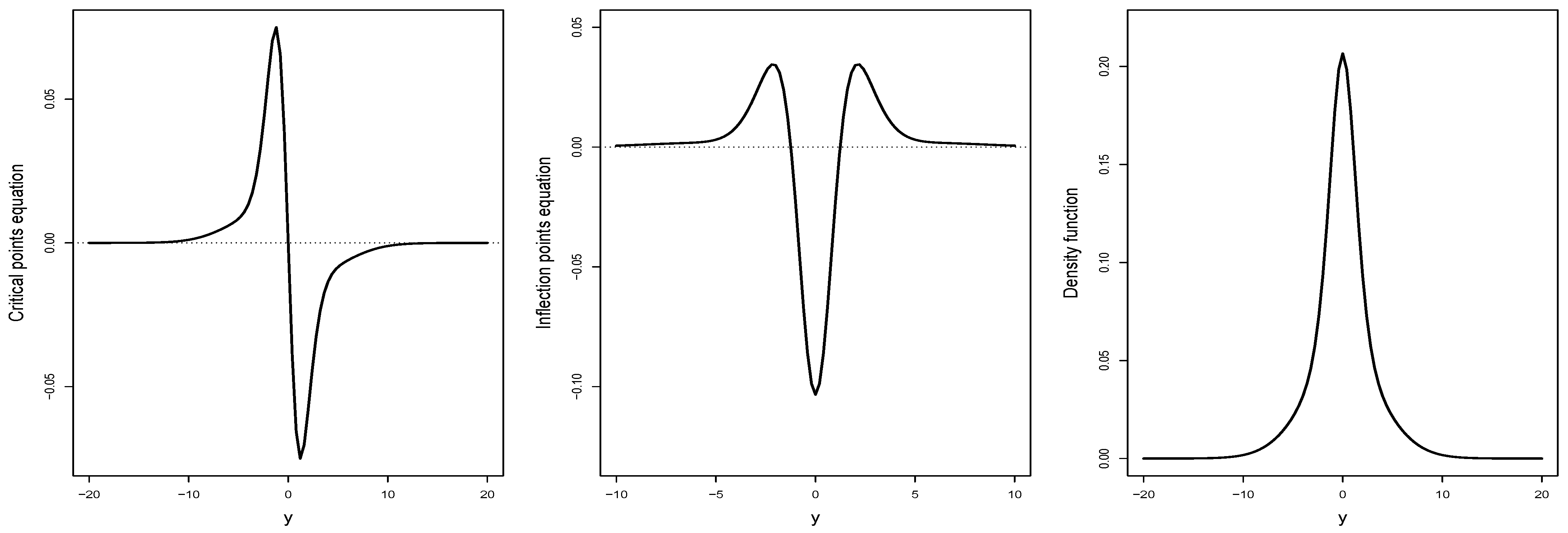
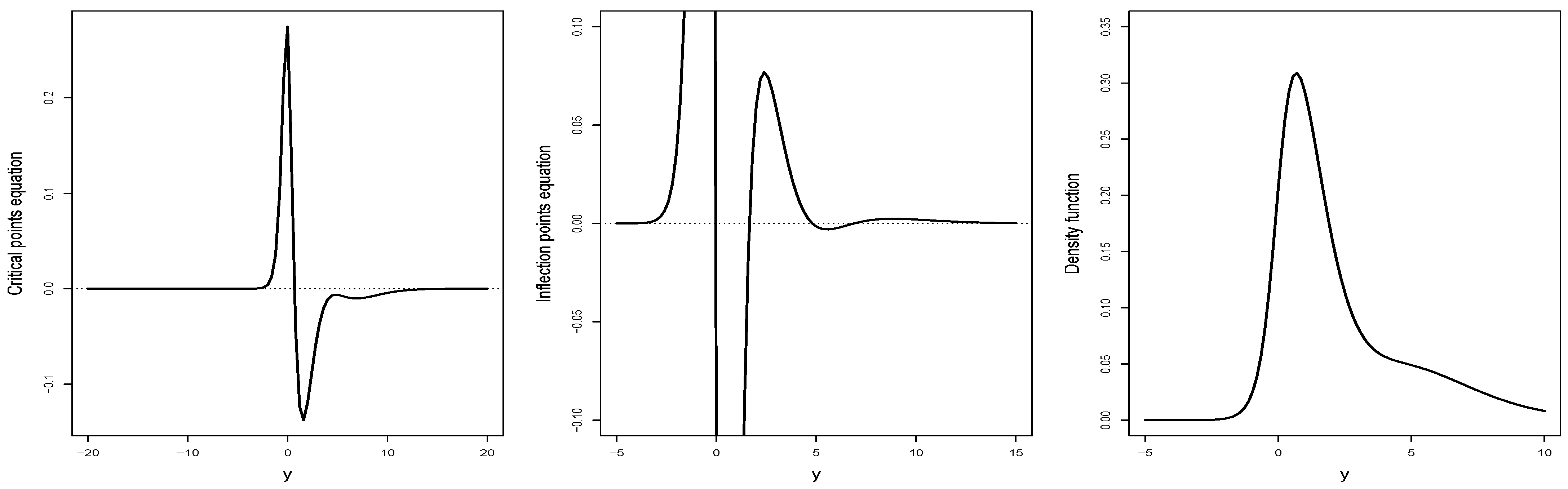
Figure 3, Figure 4, Figure 5, Figure 6 and Figure 7 present profiles of the critical points and inflection points equations (Equations (8) and (9)) and the WSLOG PDF curves considering different choices of $\lambda$ and $\alpha$. In the figures, it can be seen that the WSLOG PDF can present a unimodal shape with two, four, or six inflection points, a bimodal shape with four inflection points and a trimodal shape with six inflection points.

Considering $\lambda \in [-5,5]$ and $\alpha \in [0,5]$, Figure 8 illustrates the behavior of the WSLOG PDF in terms of the number of modes it presents. The figure reveals three differentiated regions; unimodality region, bimodality region, and a region where the PDF has three modes. Taking into account that $\lambda$ is a skewness parameter inherited from the SLOG distribution, we observe that when $\lambda =0$ (symmetric case), the WSLOG PDF is unimodal or trimodal. On the other hand, bimodal shapes are obtained when $\alpha >0$ and $\lambda \ne 0$.

2.5. Moments and Skewness Behavior

In this section, the moments of the WSLOG distribution are derived and, from these, the behavior of the skewness is described.

Proposition 4.

Let $Y\sim \mathrm{WSLOG}(\mu ,\sigma ,\lambda ,\alpha )$. Hence, for $r=1,2,3,\dots$, we have

$$\begin{array}{ccc}\hfill \mathbb{E}\left[Y^r\right]& =& \frac{1}{1+\alpha {\kappa }_{\lambda }}\left[\left(1+\frac{\alpha {\mu }_1^{\prime 4}}{{\sigma }_1^4}\right){\mu }_r^{\prime }\right.\hfill \\ \hfill & & \left.+\frac{\alpha }{{\sigma }_1^4}\left({\mu }_{r+4}^{\prime }-4{\mu }_1^{\prime }{\mu }_{r+3}^{\prime }+6{\mu }_1^{\prime 2}{\mu }_{r+2}^{\prime }-4{\mu }_1^{\prime 3}{\mu }_{r+1}^{\prime }\right)\right],\hfill \end{array}$$

(10)

where ${\kappa }_{\lambda }$ is as in Equation (4), ${\sigma }_1^2=2{\sigma }^2({\mathbb{I}}_2-{\mathbb{I}}_1^2)$ and ${\mu }_r^{\prime }={\sum }_{j=0}^r\left(\genfrac{}{}{0pt}{}{r}{j}\right){\sigma }^j{\mathbb{I}}_j{\mu }^{r-j}$, such that ${\mathbb{I}}_0=1$ and  ${\mathbb{I}}_j$, $j=1,\dots ,r$, is as in Equation (2).

Proof. 

From Equation (6), we see that

$$\begin{array}{ccc}\hfill \mathbb{E}\left[Y^r\right]& =& {\int }_{-\infty }^{\infty }\frac{y^r}{1+\alpha {\kappa }_{\lambda }}\left[1+\alpha {\left(\frac{y-{\mu }_1^{\prime }}{{\sigma }_1}\right)}^4\right]\frac{2e^{-z}}{\sigma {\left(1+e^{-z}\right)}^2\left(1+e^{-\lambda z}\right)}dy\hfill \\ & =& {\int }_{-\infty }^{\infty }\frac{1}{1+\alpha {\kappa }_{\lambda }}\left[y^r+\frac{\alpha }{{\sigma }_1^4}\left(y^{r+4}-4y^{r+3}{\mu }_1^{\prime }+6y^{r+2}{\mu }_1^{\prime 2}-4y^{r+1}{\mu }_1^{\prime 3}+y^r{\mu }_1^{\prime 4}\right)\right]\hfill \\ & & \times \frac{2e^{-z}}{\sigma {\left(1+e^{-z}\right)}^2\left(1+e^{-\lambda z}\right)}dy.\hfill \end{array}$$

Recognizing in the previous integral the r-th moment of the SLOG distribution, ${\mu }_r^{\prime }={\sum }_{j=0}^r\left(\genfrac{}{}{0pt}{}{r}{j}\right){\sigma }^j{\mathbb{I}}_j{\mu }^{r-j}$, such that ${\mathbb{I}}_r$ is as in Equation (2), we obtain that

$$\begin{array}{ccc}\hfill \mathbb{E}\left[Y^r\right]& =& \frac{1}{1+\alpha {\kappa }_{\lambda }}\left[{\mu }_r^{\prime }+\frac{\alpha }{{\sigma }_1^4}\left({\mu }_{r+4}^{\prime }-4{\mu }_{r+3}^{\prime }{\mu }_1^{\prime }+6{\mu }_{r+2}^{\prime }{\mu }_1^{\prime 2}-4{\mu }_{r+1}^{\prime }{\mu }_1^{\prime 3}+{\mu }_r^{\prime }{\mu }_1^{\prime 4}\right)\right]\hfill \\ & =& \frac{1}{1+\alpha {\kappa }_{\lambda }}\left[\left(1+\frac{\alpha {\mu }_1^{\prime 4}}{{\sigma }_1^4}\right){\mu }_r^{\prime }+\frac{\alpha }{{\sigma }_1^4}\left({\mu }_{r+4}^{\prime }-4{\mu }_1^{\prime }{\mu }_{r+3}^{\prime }+6{\mu }_1^{\prime 2}{\mu }_{r+2}^{\prime }-4{\mu }_1^{\prime 3}{\mu }_{r+1}^{\prime }\right)\right].\hfill \end{array}$$

which is the result given in Equation (10).    □

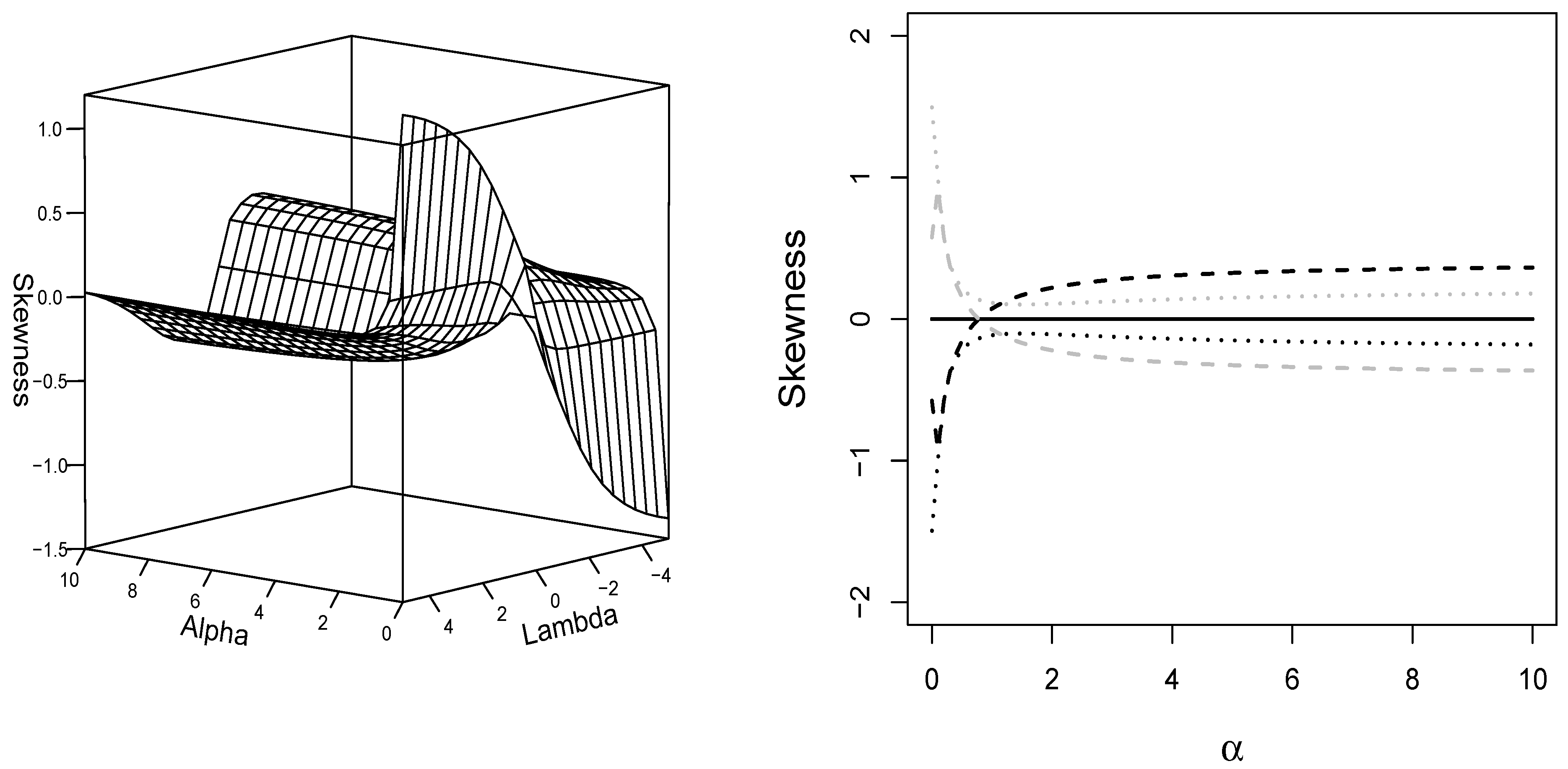
Corollary 4.

Let $Y\sim \mathrm{WSLOG}(\mu ,\sigma ,\lambda ,\alpha )$. Then, the mean ($\mathbb{E}\left(Y\right)$), variance ($\mathbb{V}ar\left(Y\right)$), and Fisher’s skewness (S) and kurtosis (K) coefficients of Y are

$$\begin{array}{ccc}\hfill \mathbb{E}\left(Y\right)& =& {\mu }_1,\hfill \\ \hfill \mathbb{V}ar\left(Y\right)& =& {\mu }_2-{\mu }_1^2,\hfill \\ \hfill S& =& \frac{{\mu }_3-3{\mu }_1{\mu }_2+2{\mu }_1^3}{{({\mu }_2-{\mu }_1^2)}^{3/2}}\hfill \\ \hfill \mathit{and}\\ \hfill K& =& \frac{{\mu }_4-4{\mu }_1{\mu }_3+6{\mu }_1^2{\mu }_2-3{\mu }_1^4}{{({\mu }_2-{\mu }_1^2)}^2},\hfill \end{array}$$

where

$$\begin{array}{ccc}\hfill {\mu }_1& =& \frac{1}{1+\alpha {\kappa }_{\lambda }}\left[\left(1+\frac{\alpha {\mu }_1^{\prime 4}}{{\sigma }_1^4}\right){\mu }_1^{\prime }+\frac{\alpha }{{\sigma }_1^4}\left({\mu }_5^{\prime }-4{\mu }_1^{\prime }{\mu }_4^{\prime }+6{\mu }_1^{\prime 2}{\mu }_3^{\prime }-4{\mu }_1^{\prime 3}{\mu }_2^{\prime }\right)\right],\hfill \end{array}$$

$$\begin{array}{ccc}\hfill {\mu }_2& =& \frac{1}{1+\alpha {\kappa }_{\lambda }}\left[\left(1+\frac{\alpha {\mu }_1^{\prime 4}}{{\sigma }_1^4}\right){\mu }_2^{\prime }+\frac{\alpha }{{\sigma }_1^4}\left({\mu }_6^{\prime }-4{\mu }_1^{\prime }{\mu }_5^{\prime }+6{\mu }_1^{\prime 2}{\mu }_4^{\prime }-4{\mu }_1^{\prime 3}{\mu }_3^{\prime }\right)\right],\hfill \\ \hfill {\mu }_3& =& \frac{1}{1+\alpha {\kappa }_{\lambda }}\left[\left(1+\frac{\alpha {\mu }_1^{\prime 4}}{{\sigma }_1^4}\right){\mu }_3^{\prime }+\frac{\alpha }{{\sigma }_1^4}\left({\mu }_7^{\prime }-4{\mu }_1^{\prime }{\mu }_6^{\prime }+6{\mu }_1^{\prime 2}{\mu }_5^{\prime }-4{\mu }_1^{\prime 3}{\mu }_4^{\prime }\right)\right],\hfill \\ \hfill {\mu }_4& =& \frac{1}{1+\alpha {\kappa }_{\lambda }}\left[\left(1+\frac{\alpha {\mu }_1^{\prime 4}}{{\sigma }_1^4}\right){\mu }_4^{\prime }+\frac{\alpha }{{\sigma }_1^4}\left({\mu }_8^{\prime }-4{\mu }_1^{\prime }{\mu }_7^{\prime }+6{\mu }_1^{\prime 2}{\mu }_6^{\prime }-4{\mu }_1^{\prime 3}{\mu }_5^{\prime }\right)\right],\hfill \end{array}$$

such that ${\mu }_j^{\prime }$, with $j=1,2,3,4$, is as in Equation (10).

Figure 9 presents 3-D and 2-D perspectives for the Fisher’s skewness coefficient of the WSLOG distribution. From the figure, we note the following: (1) From the 2-D perspective, it can be seen that if $\lambda =0$, then the WSLOG PDF is symmetric. (2) From the 3-D perspective, it can be seen that the highest skewness values are obtained when considering small values of $\alpha$ (close to 0) and high values of $\lambda$; that is, in the unimodal case, by complementing this with the results obtained from Figure 8. (3) In both perspectives, it can be seen that for a fixed $\lambda$, the skewness can increase or decrease as $\alpha$ grows. However, we can note that $\alpha$ has a smooth effect on the skewness.

2.6. Possible Application Scenarios

Focusing on the PDF shapes described in Section 2.4, we next consider some possible application scenarios for the WSLOG distribution.

For the unimodal case, there are many possible scenarios of application that we can mention. We considered the following: (1) Hydrology: to model hydrological variables such as river flows and water levels. These variables often exhibit unimodality and asymmetry. (2) Economy and Finance: to model asset returns, volatility, and other financial data that may exhibit unimodal and asymmetric behavior. (3) Environment: to model data related to air pollution, concentrations of chemical substances, and other types of environmental data. (4) Demography and Social Sciences: to model data such as the age distribution of a population, migration rates, and other demographic variables.

In general, the WSLOG distribution, in its unimodal shape, can be considered an alternative distribution for data modeling in scenarios where the skew-logistic distribution is used. The fact that the PDF WSLOG can have more than two inflection points (in its unimodal shape) can lead to better fits of datasets whose frequency distributions are unimodal but with extravagant shapes.

Focusing on the bimodal shapes, we believe that the WSLOG distribution can be considered a viable alternative for modeling data associated with environmental variables. When analyzing this type of variable, it is common to find data that exhibit bimodality due to factors such as special geographic characteristics and seasonality. For example, the wind speed in the Canary Islands may exhibit bimodality due to the interaction of the trade winds with the mountainous and volcanic topography of this region. This can cause local disturbances in certain areas, which increases the wind speed in those specific areas, see [14]. Another example that we can mention is related to the behavior of the distribution of rainfall in Central America. In this region, precipitation shows a bimodal behavior related to the influence of the rainy seasons in the Caribbean and the Pacific, see [15].

Both in the bimodal and trimodal case, the WSLOG distribution can be used to analyze data in scenarios where it is possible to identify sub-populations with differentiated behavior with respect to the characteristic of interest studied in the population. In this case, the WSLOG distribution can be considered an alternative to the popular mixture models, especially the logistic mixture model.

3. Parameter Estimation

The problem of estimating parameters for the WSLOG distribution using the maximum likelihood method is discussed in this section. In addition, simulation experiments are carried out to assess the performance of the estimators.

3.1. Maximum Likelihood Estimators

For a random sample $Y_1,\dots ,Y_n$ of the $\mathrm{WSLOG}\left(\mathit{\theta }\right)$ distribution, with $\mathit{\theta }=(\mu ,\sigma ,\lambda ,\alpha )$. Then, the log-likelihood function associated with $\mathit{\theta }$ is written as

$$\begin{array}{ccc}\hfill \mathsf{\ell }(\mathit{\theta };\mathbf{y})& =& n\log \left(2\right)-n\log \left(\sigma \right)-n\log (1+\alpha {\kappa }_{\lambda })+\sum _{i=1}^n\log \left(1+\alpha z_{1i}^4\right)\hfill \\ \hfill & & -\sum _{i=1}^n{z}_i-2\sum _{i=1}^n\log \left(1+e^{-z_i}\right)-\sum _{i=1}^n\log (1+e^{-\lambda z_i}),\hfill \end{array}$$

(11)

where $\mathbf{y}={(y_1,\dots ,y_n)}^{\top }$ are the vector of observed values, $z_i=(y_i-\mu )/\sigma$ and $z_{1i}=(y_i-{\mu }_1^{\prime })/{\sigma }_1$, for $i=1,\dots ,n$. Thus, the elements of the score vector associated with the log-likelihood function (11) are given by

$$\begin{array}{ccc}\hfill \frac{\mathsf{\partial }\mathsf{\ell }(\mathit{\theta };\mathbf{y})}{\mathsf{\partial }\mu }& =& -\frac{4\alpha }{\sqrt{2{\sigma }^2({\mathbb{I}}_2-2{\mathbb{I}}_1^2)}}\sum _{i=1}^n\frac{z_{1i}^3}{(1+\alpha z_{1i}^4)}-\frac{2}{\sigma }\sum _{i=1}^n\frac{\exp (-z_i)}{(1+\exp (-z_i))}\hfill \\ & & -\frac{\lambda }{\sigma }\sum _{i=1}^n\frac{\exp (-\lambda z_i)}{(1+\exp (-\lambda z_i))}+\frac{n}{\sigma },\hfill \\ \hfill \frac{\mathsf{\partial }\mathsf{\ell }(\mathit{\theta };\mathbf{y})}{\mathsf{\partial }\sigma }& =& -\frac{n}{\sigma }+\sum _{i=1}^n\frac{z_i}{\sigma }-\frac{2}{\sigma }\sum _{i=1}^n\frac{z_i\exp (-z_i)}{(1+\exp (-z_i))}\hfill \\ & & -\frac{\lambda }{\sigma }\sum _{i=1}^n\frac{z_i\exp (-\lambda z_i)}{(1+\exp (-\lambda z_i))}-\frac{4\alpha }{\sqrt{2{\sigma }^2({\mathbb{I}}_2-2{\mathbb{I}}_1^2)}}\sum _{i=1}^n\frac{z_{1i}^3{z}_i}{(1+\alpha z_{1i}^4)},\hfill \\ \hfill \frac{\mathsf{\partial }\mathsf{\ell }(\mathit{\theta };\mathbf{y})}{\mathsf{\partial }\lambda }& =& \sum _{i=1}^n\frac{z_i\exp (-\lambda z_i)}{(1+\exp (-\lambda z_i))},\hfill \\ \hfill \frac{\mathsf{\partial }\mathsf{\ell }(\mathit{\theta };\mathbf{y})}{\mathsf{\partial }\alpha }& =& \sum _{i=1}^n\frac{z_{1i}^4}{(1+\alpha z_{1i}^4)}-\frac{n{\kappa }_{\lambda }}{(1+\alpha {\kappa }_{\lambda })}.\hfill \end{array}$$

Since the ML estimators of $\mu$, $\sigma$, $\alpha$, and $\lambda$ do not have closed expressions, it is necessary to use numerical procedures such as Newton–Raphson.

The standard errors of the ML estimators can be obtained as the square roots of the elements of the diagonal of the matrix

$$\begin{array}{ccc}\hfill {\mathbf{K}}^{-1}\left(\widehat{\mathit{\theta }}\right)& =& {\left\{-\frac{{\mathsf{\partial }}^2\mathsf{\ell }(\mathit{\theta };\mathbf{y})}{\mathsf{\partial }\mathit{\theta }\mathsf{\partial }{\mathit{\theta }}^{\top }}{|}_{\begin{array}{c}\mathit{\theta }=\widehat{\mathit{\theta }}\end{array}}\right\}}^{-1},\hfill \end{array}$$

where ${\mathsf{\partial }}^2\mathsf{\ell }(\mathit{\theta };\mathbf{y})/\mathsf{\partial }\mathit{\theta }\mathsf{\partial }{\mathit{\theta }}^{\top }$ is the Hessian matrix.

Alternatively, it is possible to solve the problem of maximizing Equation (11) with the help of some numerical optimization routine such as the function stats:optim() of the R programming language [16]. In this case, minimizing the negative log-likelihood, this function returns the ML estimates and the numerical Hessian matrix. The R code used is available at https://github.com/isaaccortes1989/WSLOG-ARTICLE, accessed on 20 March 2024.

3.2. Simulation Study

In this section, we carry out a simulation study aimed at evaluating the behavior of the ML estimators of the parameters of the WSLOG distribution.

3.2.1. Simulation Algorithm

We used the accept-reject method to generate pseudo-random numbers from the WSLOG distribution. The results in a sequence of n pseudo-random numbers were stored inside an array that we called $n_{vector}$. We considered the envelope function $g\left(x\right)=cf(x;m,s)$, where $f(x;m,s)=e^{-(x-m)/s}{[1+e^{-(x-m)/s}]}^{-2}$, $x,m\in \mathbb{R}$, $s>0$, is the PDF of the logistic distribution. Thus, from Equation (6), to determine the value of the constant c, we calculated the root of the equation

$$\begin{array}{ccc}\hfill 0& =& \frac{\mathsf{\partial }}{\mathsf{\partial }x}\frac{\left[1+\alpha {\left(\frac{x-{\mu }_1^{\prime }}{{\sigma }_1}\right)}^4\right]e^{-\frac{x-\mu }{\sigma }}{\left(1+e^{-\frac{x-m}{s}}\right)}^2}{{\left(1+e^{-\frac{x-\mu }{\sigma }}\right)}^2\left(1+e^{-\lambda \frac{x-\mu }{\sigma }}\right)e^{-\frac{x-m}{s}}}.\hfill \end{array}$$

(12)

In addition to the parameters $\mu$, $\sigma$, $\lambda$ and $\alpha$ of the WSLOG distribution, to build the algorithm (Algorithm 1), we needed to define:

• n: The length of the $n_{vector}$.
• $\mu$, $\sigma$, $\lambda$ y $\alpha$: The parameters of the WSLOG distribution.
• m y s: The location and scale parameters of the logistic distribution.
• $f_Y(·;\mu ,\sigma ,\lambda ,\alpha )$: The WSLOG PDF whit $\mu \in \mathbb{R}$, $\sigma >0$, $\lambda \in \mathbb{R}$ and $\alpha >0$.
• $f(·;m,s)$: The logistic PDF with $m\in \mathbb{R}$ and $s>0$.
• $U_1$: A random variable with a uniform$(0,1)$ distribution.
• $U_2$: A random variable with a uniform$(0,1)$ distribution.

Algorithm 1: Accept-Reject Algorithm to Generate Pseudo Random Numbers from the WSLOG$(\mu ,\sigma ,\lambda ,\alpha )$ Distribution.

3.2.2. Simulation Scenarios

We focused on two different choices for the parameter vector $\theta =(\mu ,\sigma ,\lambda ,\alpha )$ of the WSLOG distribution, thus defining the following simulation scenarios:

• Scenario A, $\theta =(10,2,-0.3,0.2)$: this choice of $\theta$ leads to a PDF with an asymmetric unimodal shape, with six inflection points. To generate pseudo-random numbers from the WSLOG distribution, we solved Equation (12) considering $m=6$ and $s=10$, obtaining $c=3.284$.
• Scenario B, $\theta =(30,3,-3,5)$: this choice of $\theta$ leads to a PDF with an asymmetric bimodal shape. In this case, we solved the Equation (12) considering $m=18$ and $s=5.4$, obtaining $c=2.0436$.

The values of the parameters that give rise to Scenarios 1 and 2 were selected through a graphical inspection of the WSLOG PDF, so that the simulation aims to consider pseudo-random numbers that come from an asymmetric unimodal population (Scenario 1) and an asymmetric bimodal population (Scenario 2).

Figure 10 presents the WSLOG PDF curves with the envelope functions considered in both simulation scenarios.

3.2.3. Results

We generated 1000 pseudo-random samples from the WSLOG distribution for the scenarios described above, under the sample sizes n = 100, 150, 200, …, and 750, respectively. Subsequently, we obtained the ML estimates with their corresponding standard errors and squared errors.

Figure 11 and Figure 12 illustrate the behavior of the mean estimate (Mean), standard deviation (SD), root mean square error (RMSE), asymptotic standard error (SE), and probability of coverage (CP) of the 95% asymptotic confidence intervals that were obtained under the different sample sizes considered in the two simulation scenarios. In the figures, it can be seen that, as the sample size increases, the mean estimates get closer to the true values of the parameters and the SDs, SEs, and RMSEs decrease and tend to be close to each other, which suggests the asymptotic consistency of the estimators. In addition, we observe that the CPs approach nominal values as the sample size increases.

4. Data Analysis

Environmental data allow us to monitor the state of our natural environment, including air quality, water quality, biodiversity, temperature, among other factors. Continuous probability distributions have played an important role in the analysis of problems involving environmental variables. For example, Kassem et al. [17] investigated the wind characteristics and available wind energy for three urban regions in Northern Cyprus using the Weibull distribution; Rad et al. [18] proposed a mixture of multimodal skewed von Mises to model the wind direction in different geographic regions of interest under a Bayesian approach; Suleiman et al. [19] proposed the odd beta prime-logistic distribution to evaluate magnesium concentrations for groundwater quality.

This section illustrates the usefulness of the WSLOG distribution by fitting two real datasets associated with environmental variables.

4.1. Fitted Distributions

We compared the performance of the WSLOG distribution with that of the logistic mixture model and other bimodal distributions popular in the literature. Below is the PDF of each distribution considered:

• Logistic mixture (MLOG) PDF [5]

  $$\begin{array}{c}\hfill f(x;\mu ,\sigma ,{\mu }_2,{\sigma }_2,\alpha )=\frac{\alpha }{\sigma }\frac{e^{\frac{x-\mu }{\sigma }}}{{\left(1+e^{\frac{x-\mu }{\sigma }}\right)}^2}+\frac{1-\alpha }{{\sigma }_2}\frac{e^{\frac{x-{\mu }_2}{{\sigma }_2}}}{{\left(1+e^{\frac{x-{\mu }_2}{{\sigma }_2}}\right)}^2},x\in \mathbb{R},\end{array}$$

  where $\mu ,{\mu }_2\in \mathbb{R}$ are the locations of the mixture components, $\sigma ,{\sigma }_2>0$ are the scales of the mixture components, and $\alpha \in (0,1)$ is the mixing parameter.
• Skew bimodal-logistic (SBLOG) PDF [20]

  $$\begin{array}{c}\hfill f(x;\mu ,\sigma ,\lambda ,\alpha )=\frac{6}{{\sigma }^3}\left(\frac{{\sigma }^2+\alpha {(x-\mu )}^2}{3+{\pi }^2\alpha }\right)\frac{e^{\frac{x-\mu }{\sigma }}}{{\left(1+e^{\frac{x-\mu }{\sigma }}\right)}^2}\frac{e^{\lambda \frac{x-\mu }{\sigma }}}{(1+e^{\lambda \frac{x-\mu }{\sigma }})},x\in \mathbb{R},\end{array}$$

  where $\mu \in \mathbb{R}$ is a location parameter, $\sigma >0$ is a scale parameter, $\lambda \in \mathbb{R}$, and $\alpha >0$ are shape parameters that control skewness and uni/bi-modality.
• Skew flexible normal (SFN) PDF [9]

  $$\begin{array}{c}\hfill f(x;\mu ,\sigma ,\lambda ,\alpha )=\frac{c_{\alpha }}{\sigma }\varphi \left(\left|\frac{x-\mu }{\sigma }\right|+\alpha \right)\Phi \left(\lambda \frac{x-\mu }{\sigma }\right),x\in \mathbb{R},\end{array}$$

  where $\mu \in \mathbb{R}$ is a location parameter, $\sigma >0$ is a scale parameter, $\alpha ,\lambda \in \mathbb{R}$ are shape parameters that control skewness and uni/bi-modality, $c_{\alpha }^{-1}=[1-\Phi \left(\alpha \right)]$ is a normalizing constant, and $\varphi (·)$ and $\Phi (·)$ are the PDF and CDF of the standard normal distribution, respectively.
• Asymmetric bimodal power normal (ABPN) PDF [11]

  $$\begin{array}{c}\hfill f(x;\mu ,\sigma ,\lambda ,\alpha )=\frac{2\alpha c_{\alpha }}{\sigma }\varphi \left(\frac{x-\mu }{\sigma }\right)\Phi {\left(\left|\frac{x-\mu }{\sigma }\right|\right)}^{\alpha -1}\Phi \left(\lambda \frac{x-\mu }{\sigma }\right),x\in \mathbb{R},\end{array}$$

  where $\mu \in \mathbb{R}$ is a location parameter, $\sigma >0$ is a scale parameter, $\lambda \in \mathbb{R}$ and $\alpha >0$ are shape parameters that control skewness and uni/bi-modality, $c_{\alpha }=2^{\alpha -1}/(2^{\alpha }-1)$ is a normalizing constant, and $\varphi (·)$ and $\Phi (·)$ are the PDF and CDF of the standard normal distribution, respectively.

The PDFs described above exhibit uni/bimodal asymmetric shapes depending on the values assumed by their shape parameters. Note, however, that the MLOG distribution has a larger parameter dimension, which translates into more shape flexibility for the PDF, but at the cost of investing more effort in parameter estimation. On the other hand, the SBLOG, SFN, and ABPN distributions have the same parameter dimension as the WSLOG distribution, so the WSLOG distribution can be considered a natural alternative for data modeling in scenarios where the SBLOG, SFN, and ABPN distributions are employed.

4.2. Fit Measurements

We used the Anderson–Darling (AD) and Cramér-von Mises (CvM) goodness-of-fit tests to assess the quality of fit of the WSLOG distribution. For this, we used the functions goftest::ad.test() and goftest::cvm.test() in the R programming language, see [21]. To assess comparative performance, we considered the Akaike Information Criterion (AIC) [22], the Corrected Akaike Information Criterion (CAIC) [23], and the Bayesian Information Criterion (BIC) [24]. These criteria are defined as $\mathrm{AIC}=2k-2\mathsf{\ell }$, $\mathrm{CAIC}=k\left[\log \right(n)+1]-2\mathsf{\ell }$, $\mathrm{BIC}=k\log \left(n\right)-2\mathsf{\ell }$, respectively, where k is the number of parameters to be estimated, n is the sample size, and ℓ is the maximum log-likelihood value.

4.3. Unimodality Test

In order to achieve a deep understanding of the behavior of empirical frequency distributions, in addition to justifying the relevance of postulating the WSLOG distribution as a viable candidate for data modeling, we tested the hypothesis ${\mathrm{H}}_0$: the data have exactly one mode, versus the hypothesis ${\mathrm{H}}_1$: the data have at least two modes. For this, we consider the excess mass test using the function multimode::modetest() in the R programming language, see [25] and [26].

4.4. Data Description

Details of the analyzed datasets are provided below.

4.4.1. Geometric Features of Pollen Grains

The pollen grain is a fundamental structure in the reproduction of flowering plants. Its cellular and structural composition allows it to transport male genetic material to the female reproductive organs of the flower. Geometric characteristics of the pollen grain, such as its shape, size, and presence of surface structures, play an important role in studies on the growth of flowering plants. For this reason, we studied 481 observations on the measurement of a surface feature (ridge) along a direction in a certain type of pollen grain. These data are available on the website http://lib.stat.cmu.edu/datasets/pollen.data, accessed on 20 March 2024. Specifically, the data correspond to the observations of the variable “Ridge” in the data file POLLEN1.DAT.

Computing some descriptive measures, we saw that the minimum and maximum observations were −19.4687 and 21.4066, respectively, and that Fisher’s skewness coefficient was 0.0246, a smooth skewness level. In the excess mass test, we obtained an observed statistic of value 0.219, with a corresponding p-value equal to 0.164, which led us to conclude (at a significance level of 5%) that the frequency distribution of the data was unimodal. Taking these results into account, we explored the performance of the WSLOG distribution in fitting this dataset.

4.4.2. Temperature of Administrative Regions with Prevalence of Dengue

Dengue is a viral disease transmitted mainly by mosquitoes of the Aedes genus, endemic in many tropical and subtropical areas of the world. Ambient temperature plays a crucial role in the spread and incidence of dengue, since it affects both the vector mosquitoes and the virus; high temperatures positively influence the rate of development and reproduction of mosquitoes and favor the replication of the virus in them. We analyzed a dataset containing 1998 observations on the average temperature in administrative areas where occurrences of dengue virus have been documented. For more information regarding this dataset, please consult [27], or access it within the “dengue” database under the identifier “temp“ in the R software, version 4.3.1, as indicated in [28].

In the excess mass test, the observed statistic was equal to 0.048, with a p-value less than 0.01, which allowed us to conclude with a significance level of 1% that the temperature data are at least bimodal. Adding to the above the fact that the Fisher skewness coefficient was −0.728, a negative skewness level, we believe that the WSLOG distribution is a viable alternative for fitting the temperature data.

4.5. Results

Table 1. ML estimates for the parameters of the distributions fitted to the data described in Section 4.4.

Ridge Variable
Estimate	WSLOG	MLOG	SBLOG	SFN	ABPN
$\widehat{\mu }$	−1.458 (0.396)	−1.207 (1.050)	2.612 (0.796)	2.464 (0.725)	−1.294 (0.156)
$\widehat{\sigma }$	1.558 (0.065)	3.231 (0.307)	2.241 (0.150)	6.176 (0.543)	7.528 (0.831)
${\widehat{\mu }}_2$	-	7.279 (1.702)	-	-	-
${\widehat{\sigma }}_2$	-	1.996 (0.801)	-	-	-
$\widehat{\lambda }$	0.182 (0.067)	-	−0.264 (0.107)	−0.417 (0.158)	0.353 (0.088)
$\widehat{\alpha }$	0.255 (0.034)	0.831 (0.135)	0.376 (0.092)	−0.214 (0.189)	0.363 (0.270)
AIC	3141.8	3151.9	3148.4	3150.8	3149.5
CAIC	3162.5	3177.8	3169.1	3171.5	3170.2
BIC	3158.5	3172.8	3165.1	3167.5	3166.2
Temp Variable
$\widehat{\mu }$	27.604 (0.082)	12.529 (0.395)	15.736 (0.206)	28.177 (0.092)	28.120 (0.093)
$\widehat{\sigma }$	2.746 (0.046)	3.842 (0.141)	2.553 (0.040)	16.202 (1.081)	14.010 (0.375)
${\widehat{\mu }}_2$	-	25.230 (0.131)	-	-	-
${\widehat{\sigma }}_2$	-	1.248 (0.071)	-	-	-
$\widehat{\lambda }$	−5.948 (0.474)	-	0.202 (0.022)	−22.942 (2.461)	−19.224 (1.856)
$\widehat{\alpha }$	0.119 (0.007)	0.530 (0.021)	1.671 (0.187)	0.644 (0.178)	$6.967\times {10}^{-4}$ (0.189)
AIC	13,031.1	13,182.3	13,650.2	13,220.1	13,205.2
CAIC	13,057.5	13,215.3	13,676.6	13,246.5	13,231.6
BIC	13,053.5	13,210.3	13,672.6	13,242.5	13,227.6

reports the ML estimates of the parameters of the distributions fitted to the data described in Section 4.4. In the tables, it can be seen that the WSLOG distribution presents the lowest values of AIC, CAIC, and BIC, which suggests that this distribution should be selected to fit both datasets.

Table 2. Goodness-of-fit tests for the WSLOG distribution fitted to the data described in Section 4.4.

Data	AD Test		CvM Test
	Statistic	$\mathit{p}$-Value	Statistic	$\mathit{p}$-Value
Ridge variable	3.578	0.272	0.703	0.228
Temp variable	3.076	0.683	0.530	0.778

shows the results of the AD and CvM goodness-of-fit tests for the WSLOG distribution fitted to the data. From the table, it can be concluded (with a significance level of 1%) that the data come from a WSLOG population with parameters specified in Table 1. Figure 13 shows the histograms of the datasets along with the fitted PDFs. Here, it is evident that the observed relative frequencies closely align with the density values of the WSLOG distribution.

The datasets and results presented in this section can be accessed at https://github.com/isaaccortes1989/WSLOG-ARTICLE, accessed on 20 March 2024.

5. Final Comments

We have proposed an extension of the skew-logistic distribution capable of presenting asymmetric shapes with up to three modes for its PDF. The new distribution corresponds to a weighted version of the skew-logistic distribution, defined by a weight function that induces an extra shape parameter. Thus, the new distribution, which we call the weighted skew-logistic (WSLOG) distribution, has two shape parameters that lead to a more flexible PDF than the skew-logistic PDF. This flexibility allows for overcoming the limitation of the use of the skew-logistic distribution to unimodal data, being the WSLOG distribution capable of modeling data that exhibit bimodality and even trimodality.

We described some possible application scenarios of the WSLOG distribution, of which we highlight its possible use in the modeling of bimodal data associated with environmental variables. Also, we derived fundamental properties such as the cumulative distribution function and raw moments. In addition, we described the behavior of the skewness of the distribution and determine the approximate regions of uni/bi and trimodality in the two-dimensional parameter space associated with the shape parameters of the distribution. Furthermore, we observed that the shape parameter inherited from the skew-logistic distribution had an important effect on the skewness of the distribution, while the shape parameter induced by the weight function had an important effect on the number of modes that the distribution presents.

We explored the issue of parameter estimation for the WSLOG distribution using the maximum likelihood approach. We carried out a simulation study to empirically evaluate the performance of the estimators. Overall, we found that the maximum likelihood method yields were satisfactory.

Finally, we presented two applications for real data associated with environmental variables; ambient temperature in administrative regions in which dengue virus cases have been recorded, and the measurement of a surface characteristic of a certain type of pollen grain. The performance of the WSLOG distribution was compared to that of some bimodal skewed distributions in the literature, including a logistic mixture model. The results suggest that the WSLOG distribution performs better in fitting both data sets, illustrating the utility of the new distribution in modeling environmental data.