Article

Fast Eigenvalue Decomposition of Arrowhead and Diagonal-Plus-Rank-k Matrices of Quaternions

by
Thaniporn Chaysri
,
Nevena Jakovčević Stor
and
Ivan Slapničar
*
Faculty of Electrical Engineering, Mechanical Engineering and Naval Architecture, University of Split, Rudjera Boškovića 32, 21000 Split, Croatia
*
Author to whom correspondence should be addressed.
Mathematics 2024, 12(9), 1327; https://doi.org/10.3390/math12091327
Submission received: 21 February 2024 / Revised: 19 April 2024 / Accepted: 23 April 2024 / Published: 26 April 2024
(This article belongs to the Section Computational and Applied Mathematics)

Abstract

:
Quaternions are a non-commutative associative number system that extends complex numbers, first described by Hamilton in 1843. We present algorithms for solving the eigenvalue problem for arrowhead and DPRk (diagonal-plus-rank-k) matrices of quaternions. The algorithms use the Rayleigh Quotient Iteration with double shifts (RQIds), Wielandt’s deflation technique and the fact that each eigenvector can be computed in O ( n ) operations. The algorithms require O ( n 2 ) floating-point operations, n being the order of the matrix. The algorithms are backward stable in the standard sense and compare well to the standard QR method in terms of speed and accuracy. The algorithms are elegantly implemented in Julia, using its polymorphism feature.

1. Introduction and Definitions

In linear algebra, there are various methods for computing eigenvalues and eigenvectors of real and complex matrices. When this problem extends to matrices of quaternions, many researchers attempt to solve it [1,2,3,4,5,6,7,8]. For the matrices of quaternions, the majority of classic methods need to be modified since quaternions are non-commutative systems and matrices of quaternions do not have the characteristic polynomial. In this paper, we use the Rayleigh Quotient Iteration with double shifts and a deflation method to solve the eigenvalue problem for the arrowhead and DPRk (diagonal-plus-rank-k) matrices of quaternions. Such matrices appear in many applications and they are parts of many significant linear algebra algorithms (see [9,10,11,12,13,14] for more information).
This paper is organized as follows. In Section 1, we give basic definitions and preliminary results. In Section 2, we give methods for the eigenvalue decomposition of matrices of quaternions. We first briefly describe the standard quaternion QR method for general matrices from [1]. We then describe our new method for arrowhead and DPRk matrices in detail. In Section 3, we analyze the error of our algorithms and show that they are backward stable. In Section 4, we give the numerical examples and compare our method with the standard quaternion QR method. We also present a discussion and conclusions in Section 5.

1.1. Quaternions

Quaternions are a non-commutative associative number system that extends complex numbers, introduced by Hamilton [15,16]. For basic quaternions  i , j and  k , the quaternions have the form
q = a + b i + c j + d k , a , b , c , d , R .
The multiplication table of basic quaternions is the following:
× i j k i 1 k j j k 1 i k j i 1
Conjugation is given by
q ¯ = a b i c j d k .
Then,
q ¯ q = q q ¯ = | q | 2 = a 2 + b 2 + c 2 + d 2 .
Also, the real and the imaginary parts of q are defined by
real ( q ) = q + q ¯ 2 = a , imag ( q ) = q q ¯ 2 ,
respectively.
The dot product of two vectors of quaternions p , q H n , is defined in the standard manner:
p · q = i = 1 n p ¯ i q i .
Let f ( x ) be a complex analytic function. The value f ( q ) , where q H , is computed by evaluating the extension of f to the quaternions at q (see [17]). All of the above is implemented in the Julia [18] package Quaternions.jl [19]. Quaternions are homomorphic to C 2 × 2 :
q a + b i c + d i c + d i a b i C ( q ) ,
with eigenvalues q s and q ¯ s .

1.2. Matrices of Quaternions

Let H be a set of quaternions. Any matrix A = B 1 + B 2 i + B 3 j + B 4 k H n × n , where B i R n × n , i = 1 , 2 , 3 , 4 can be uniquely expressed as
( B 1 + B 2 i ) + ( B 3 + B 4 i ) j A 1 + A 2 j , A 1 , A 2 C n × n .
Similarly, matrices of quaternions are homomorphic to C 2 n × 2 n :
A A 1 A 2 A 2 ¯ A 1 ¯ .
Notice that
A 1 = real ( A ) real ( A i ) i , A 2 = real ( A j ) real ( A k ) i .
The right eigenvalues and the standard right eigenvalues of the matrix A are defined by:
Λ ( A ) = { λ H : A x = x λ for some x H n , x 0 } , Λ s ( A ) = { λ C : A x = x λ for some x H n , x 0 , imag ( λ ) 0 } .
Let ( λ , x ) be the right eigenpair of A where λ is the standard eigenvalue. Then, λ is invariant under similarity with complex numbers: if
A x = x λ ,
then
A ( x a ) = ( x a ) 1 a λ a = ( x a ) λ ,
for any non-zero a C .

1.3. Arrowhead and Diagonal-Plus-Rank-k Matrices

Let A * and x * denote the adjoints of matrix A and vector x, respectively.
The arrowhead matrix (Arrow) is a matrix of the form
A = D u v * α Arrow ( D , u , v , α ) ,
where D is a diagonal matrix with diagonal elements d i D i i H , diag ( D ) , u , v H n 1 and  α H or any symmetric permutation of such matrix.
The diagonal-plus-rank-k matrix (DPRk) is a matrix of the form
A = Δ + x ρ y *
where Δ is diagonal matrix with diagonal elements δ i = Δ i i H , diag ( Δ ) H n , x , y H n × k and  ρ H k × k .
The diagonal-plus-rank-one matrix (DPR1) is a special case of a DPRk matrix for k = 1 .

1.4. Fast Multiplication and Inverses of Arrow and DPRk Matrices

The fast multiplication can be computed in O ( n ) operations and the product is written in the form w = A z . It can be calculated using the following lemma.
Lemma 1
([20], Lemma 1).  Let A = A r r o w ( D , u , v , α ) H n × n be an Arrow matrix with the tip at position A i i = α and let z be a vector. Then, w = A z , where
w j = d j z j + u j z i , j = 1 , 2 , , i 1 w i = v 1 : i 1 * z 1 : i 1 + α z i + v i : n 1 * z i + 1 : n w j = u j 1 z i + d j 1 z j , j = i + 1 , i + 2 , , n .
Further, let A = D P R k ( Δ , x , y , ρ ) H n × n be a DPRk matrix, k 1 and let β = ρ ( y * z ) ρ ( y · z ) . Then, w = A z , where
w i = δ i z i + x i β , i = 1 , 2 , , n .
Inverses of Arrow and DPRk matrices are computed in O ( n ) and O ( n k 2 ) operations, respectively, and can be calculated using the following lemmas (we usually consider cases where k < < n , so we can use O ( n ) instead of O ( n k 2 ) ).
Lemma 2
([20], Lemma 4).  Let A = A r r o w ( D , u , v , α ) H n × n be a non-singular arrow matrix with the tip at the position A i i = α and let P be the permutation matrix of the permutation p = ( 1 , 2 , , i 1 , n , i , i + 1 , , n 1 ) .
If all d j 0 , then the inverse of A is a DPR1 matrix
A 1 = DPR1 ( Δ , x , y , ρ ) = Δ + x ρ y * ,
where
Δ = P D 1 0 0 0 P T , x = P D 1 u 1 , y = P D * v 1 , ρ = ( α v * D 1 u ) 1 .
If d j = 0 , then the inverse of A is an arrow matrix with the tip of the arrow at position ( j , j ) and zero at position A i i (the tip and the zero on the shaft change places). In particular, let P ^ be the permutation matrix of the permutation p ^ = ( 1 , 2 , , j 1 , n , j , j + 1 , , n 1 ) . Partition D, u and v as
D = D 1 0 0 0 0 0 0 0 D 2 , u = u 1 u j u 2 , v = v 1 v j v 2 .
Then
A 1 = P D ^ u ^ v ^ * α ^ P T ,
where
D ^ = D 1 1 0 0 0 D 2 1 0 0 0 0 , u ^ = D 1 1 u 1 D 2 1 u 2 1 u j 1 , v ^ = D 1 * v 1 D 2 * v 2 1 v j 1 , α ^ = v j * α + v 1 * D 1 1 u 1 + v 2 * D 2 1 u 2 u j 1 .
Lemma 3
([20], Lemma 5).  Let A = D P R k ( Δ , x , y , ρ ) H n × n be a non-singular DPRk matrix.
If all δ j 0 , then the inverse of A is a DPRk matrix
A 1 = DPRk ( Δ ^ , x ^ , y ^ , ρ ^ ) = Δ ^ + x ^ ρ ^ y ^ * ,
where
Δ ^ = Δ 1 , x ^ = Δ 1 x , y ^ = Δ * y , ρ ^ = ρ ( I + y * Δ 1 x ρ ) 1 .
If k = 1 and δ j = 0 , then the inverse of A is an arrow matrix with the arrow tip at position ( j , j ) . In particular, let P be the permutation matrix of the permutation p = ( 1 , 2 , , j 1 , n , j , j + 1 , , n 1 ) . Partition Δ, x and y as
Δ = Δ 1 0 0 0 0 0 0 0 Δ 2 , x = x 1 x j x 2 , y = y 1 y j y 2 .
Then,
A 1 = P D u v * α P T ,
where
D = Δ 1 1 0 0 Δ 2 1 , u = Δ 1 1 x 1 Δ 2 1 x 2 x j 1 , v = Δ 1 * y 1 Δ 2 * y 2 y j 1 , α = y j * ρ 1 + y 1 * Δ 1 1 x 1 + y 2 * Δ 2 1 x 2 x j 1 .

2. Methods for Eigenvalue Decomposition

In this section, we first describe the standard QR method for general matrices of quaternions from [1]. In Section 4, we will compare our algorithm with this method. We then describe the method that will be used to compute individual eigenpairs, the Rayleigh Quotient Iteration with double shifts. In Section 2.4, we describe the basic deflation algorithm (Wielandt’s deflation) and its adjustment for arrow and DPRk matrices. For each type of matrix, we describe the fast method to compute all eigenvectors and give a complete algorithm.

2.1. A Quaternion QR Algorithm

In [1], the authors proposed a QR type method for computing the Schur decomposition of a general matrix of quaternions. The matrix uses only unitary transformations and is thus stable.
To compute the eigenvalues decomposition of a general matrix of quaternions, we propose the following four-step algorithm based on the algorithm from [1]:
Given a matrix A H n × n ,  Algorithm 1 has four steps:
Algorithm 1 Computing all eigenpairs of a quaternion matrix
  • Require: a general matrix A H n × n
  •   1. Reduce A to Hessenberg form by Householder reflectors, X * A X = H , where X is unitary and H is an upper Hessenberg matrix.
  •   2. Compute the Schur decomposition of H, Q * H Q = T , where Q is unitary and T is upper triangular matrix with eigenvalues of A on the diagonal, Λ = diag ( T ) .
  •   3. Compute the eigenvectors V of T by solving the Sylvester equation, T V V Λ = 0 . Then, V 1 T V = Λ .
  •   4. Multiply U = X * Q * V . Then, U 1 A U = Λ is the eigenvalue decomposition of A.
The reduction of a quaternionic matrix to Hessenberg form and the solution of the Sylvester equation are computed similarly to the real or complex case. Details of the Hessenberg reduction can be found in ([1], Appendix, Algorithms 1–3).
Consider a matrix A H n × n and the shift μ H . Set
M ( A , μ ) = A 2 ( μ + μ ¯ ) A + μ μ ¯ I .
If A x = x λ , then x is also an eigenvector of M ( A , μ ) :
M ( A , μ ) x = ( A 2 ( μ + μ ¯ ) A + μ μ ¯ I ) x = x λ 2 x ( μ + μ ¯ ) λ + x μ μ ¯ = x ( λ 2 ( μ + μ ¯ ) λ + μ μ ¯ ) .
Further, for the perfect shift, μ = λ , M ( A , μ ) has a zero eigenvalue:
λ 2 ( μ + μ ¯ ) λ + μ μ ¯ = λ 2 ( λ + λ ¯ ) λ + λ λ ¯ = 0 .
The QR method from [1] applies non-real shift μ to an upper-Hessenberg matrix H by standard use of Francis double-shift on the matrix M ( H , μ ) and applying it implicitly on H. Details of the algorithm can be found in ([1], Appendix, Algorithm 4).
Since Algorithm 1 is used for general matrices, it requires O ( n 3 ) operations. The algorithm is stable and we use it in Section 4 for comparison with our method.
Julia [18] implementation of Algorithm 1 is given in the file BGBM.jl, which is available from the GitHub repository [21].

2.2. Rayleigh Quotient Iterations

The standard Rayleigh Quotient Iteration (RQI) produces sequences of shifts, approximate eigenvalues and vectors: for k = 0 , 1 , 2 ,
λ k = 1 x k * x k x k * A x k , μ k = real ( λ k ) , y k = ( A μ k I ) 1 x k , x k + 1 = y k y k .
Since the eigenvalues of matrices of quaternions are not shift-invariant, only real shifts can be used. However, this works due to the following: let the matrix A μ I , μ R , have purely imaginary standard eigenvalue i ν :
( A μ I ) x = x ( i ν ) , μ , ν R .
Then
A x = μ x + x i ν = x ( μ + i ν ) ,
so, λ = μ + i ν is an eigenvalue of A and x is its eigenvector.
The method converges, but, since only real shifts are used, the convergence is rather slow and requires a large number of iterations, so “it is too restrictive to limit shifts to real numbers” ([1], p. 89).
Due to the fast computation of inverses from Section 1.4, one step of the RQI requires O ( n ) operations for arrow and DPRk matrices. For both methods, λ k λ and x k x , where ( λ , x ) is an eigenpair of A, provided that λ has a unique real part.
The iterations are terminated when
A x k x k λ k τ ,
where τ is a user-prescribed tolerance.

2.3. Rayleigh Quotient Iterations with Double Shifts

In order to speed the convergence up, we enhance the RQI with non-real double shifts, using the approach from [1] and Section 2.1.
The Rayleigh Quotient Iteration with Double Shifts (RQIds) produces sequences of shifts and vectors
μ k = 1 x k * x k x k * A x k , y k = [ M ( A , μ k ) ] 1 x k , x k + 1 = y k y k , k = 0 , 1 , 2 , ,
where M ( A , μ k ) is defined by (5). Therefore, vector y k is the solution of the system M ( A , μ k ) y k = x k , that is
( A 2 α ^ A + β I ) y k = x k , α ^ = μ k + μ ¯ k , β = μ k μ ¯ k .
Notice that α ^ and β are real.
In order to have a fast method which requires O ( n 2 ) operations to compute all eigenvalues and eigenvectors, the RQIds should compute one eigenpair in O ( n ) operations. Therefore, Equation (7) must be solved in O ( n ) operations.
If A is an arrowhead matrix, one step of the method requires O ( n ) operations: let x k = x ξ . Then:
D u v * α D u v * α α ^ D u v * α + β I 0 0 1 y k = x χ .
Therefore,
D 2 + u v * D u + u α v * D + α v * v * u + α 2 α ^ D u v * α + β I 0 0 1 y k = x χ ,
so
D 2 α ^ D + β I + u v * D u + u ( α α ^ ) v * D + ( α α ^ ) v * v * u + ( α α ^ ) α + β y k = x χ .
The matrix C = D 2 α ^ D + β I + u v * is a DPRk (DPR1) matrix,
C = DPRk ( D 2 α ^ D + β I , u , v , 1 ) .
Multiplication of Equation (8) by the block matrix C 1 1 from the left yields
I C 1 ( D u + u ( α α ^ ) ) v * D + ( α α ^ ) v * v * u + ( α α ^ ) α + β y k = C 1 x ξ .
Let B denote the matrix on the left hand side of Equation (9). Then, B is an arrowhead matrix and, finally, y k = B 1 C 1 x ξ . Due to fast computation of inverses of arrowhead and DPRk matrices from Lemmas 2 and 3, respectively, one step of the RQIds method requires O ( n ) operations.
If A is a DPRk matrix, Equation (7) becomes
[ ( Δ + x ρ y * ) ( Δ + x ρ y * ) α ^ ( Δ + x ρ y * ) + β I ] y k = x k ,
or
[ Δ ( Δ α ^ I ) + β I + x ρ y * Δ + ( Δ x + x ρ ( y * x ) α ^ x ) ρ y * ] y k = x k .
Similarly to the arrowhead case, we solve Equation (10) accurately in two steps: let Δ ^ = Δ ( Δ α ^ I ) + β I and let
C = Δ ^ + x ρ y * Δ DPRk ( Δ ^ , x , Δ * y , ρ ) .
Then, Equation (10) becomes
C 1 M y k = C 1 x k ,
or
D y k = x ^ k ,
where D = C 1 M and x ^ k = C 1 x k , provided C is non-singular. Notice that D is a DPRk matrix,
D = DPRk ( I , C 1 [ Δ x + x ρ ( y * x ) α ^ x ] , y , ρ ) .
Since both C and D are DPRk matrices, due to the fast computation of inverses of DPRk matrices from Lemma 3, one step of the RQIds method requires O ( n ) operations.

2.4. Wielandt’s Deflation

Theorem 1.
Let A H n × n and ( λ , u ) be a right eigenpair of A. Choose z such that z * u = 1 , say z * = 1 / u 1 0 0 . Compute the deflated matrix A ˜ = ( I u z * ) A . Then, ( 0 , u ) is an eigenpair of A ˜ . Further, if  ( μ , v ) is an eigenpair of A, then ( μ , v ˜ ) , where v ˜ = ( I u z * ) v is an eigenpair of A ˜ .
Proof. 
The proof can be found in [13], but we repeat it for the sake of completeness. Using A u = u λ and z * u = 1 , the first statement holds since
A ˜ u = ( I u z * ) A u = A u u z * A u = u λ u z * u λ = 0 .
Further,
A ˜ v ˜ = ( I u z * ) A ( I u z * ) v = ( I u z * ) A v A u z * v + u z * A u z * v = ( I u z * ) v μ u λ z * v + u z * u λ z * v = v ˜ μ .
   □

2.5. Deflation for Arrow Matrices

Lemma 4.
Let A H n × n be an arrow matrix partitioned as
A = δ 0 χ 0 Δ x υ ¯ y * α ,
where χ, υ and α are scalars, x and y are vectors and Δ is a diagonal matrix. Let λ , ν u ψ , where ν and ψ are scalars and u is a vector, be an eigenpair of A. Then, the deflated matrix A ˜ has the form
A ˜ = 0 0 T w A ^
where
w = u 1 ν δ ψ 1 ν δ + υ ¯ ,
and A ^ is an arrow matrix
A ^ = Δ u 1 ν χ + x y * ψ 1 ν χ + α .
Proof. 
We have
A ˜ = 1 0 T 0 0 I 0 0 0 T 1 ν u ψ 1 ν 0 T 0 δ 0 χ 0 Δ x υ ¯ y * α = 0 0 T 0 u 1 ν I 0 ψ 1 ν 0 T 1 δ 0 χ 0 Δ x υ ¯ y * α = 0 0 T 0 u 1 ν δ Δ u 1 ν χ + x ψ 1 ν δ + υ ¯ y * ψ 1 ν χ + α ,
as desired.    □
Lemma 5.
Let A and A ^ be as in Lemma 4. If  μ , z ^ ξ ^ is an eigenpair of A ^ , then the eigenpair of A is
μ , ζ z ^ + u 1 ν ζ ξ ^ + ψ 1 ν ζ ,
where ζ is the solution of the scalar Sylvester equation
δ + χ ψ 1 ν ζ ζ μ = χ ξ ^ .
Proof. 
If μ is an eigenvalue of A ^ , it is also an eigenvalue of A ˜ and then also of A. Assume that the corresponding eigenvector of A is partitioned as ζ z ξ . By combining (11)–(13), we have
0 0 T 0 u 1 ν δ Δ u 1 ν χ + x ψ 1 ν δ + υ ¯ y * ψ 1 ν χ + α 0 0 T 0 u 1 ν I 0 ψ 1 ν 0 T 1 ζ z ξ = 0 0 T 0 u 1 ν I 0 ψ 1 ν 0 T 1 ζ z ξ μ ,
or
0 0 T 0 u 1 ν δ Δ u 1 ν χ + x ψ 1 ν δ + υ ¯ y * ψ 1 ν χ + α 0 u 1 ν ζ + z ψ 1 ν ζ + ξ = 0 u 1 ν ζ + z ψ 1 ν ζ + ξ μ .
Since the bottom right 2 × 2 matrix is A ^ , the above equation implies
z ^ ξ ^ = u 1 ν ζ + z ψ 1 ν ζ + ξ ,
which proves (14). It remains to compute ζ . The first component of equality
A ζ z ξ = δ 0 χ 0 Δ x υ ¯ y * α ζ z ξ = ζ z ξ μ
implies
δ ζ + χ ξ = ζ μ ,
or
δ ζ + χ ξ ^ + ψ 1 ν ζ = ζ μ ,
which is exactly Equation (15).    □

2.5.1. Computing the Eigenvectors of Arrow Matrices

Let λ , ν u ψ be an eigenpair of the matrix A partitioned according to Lemma 4, that is
δ 0 χ 0 Δ x υ ¯ y * α ν u ψ = ν u ψ λ .
If λ and ψ are known, then the other components of the eigenvector are solutions of scalar Sylvester equations
δ ν ν λ = χ ψ , Δ i i u i u i λ = x i ψ , i = 1 , , n 2 .
By setting
γ = δ + χ ψ 1 ν
the Sylvester Equation (15) becomes
γ ζ ζ μ = χ ξ ^ .
Dividing first the equation in (16) by ν from the right and combining with the expression for γ  gives
γ = ν λ 1 ν .

2.5.2. Complete Algorithm for Arrow Matrices

In the first (forward) pass, the absolute largest eigenvalue and its eigenvector are computed by RQIds in each step. The first element of the current vector x and the first and the last elements of the current eigenvector are stored. The current value γ is computed using (18) and stored. The deflation is then performed according to Lemma 4.
The eigenvectors are reconstructed bottom-up, that is from the smallest matrix to the original one (a backward pass). In each iteration, we need to have access to the first element of the vector x which was used to define the current arrow matrix, its absolutely largest eigenvalue and the first and the last elements of the corresponding eigenvector.
In the ith step, for each j = i + 1 , , n the following steps are performed:
  • Equation (17) is solved for ζ (the first element of the eigenvector of the larger matrix). The quantity ξ ^ is the last element of the eigenvectors and was stored in the forward pass.
  • The first element of the eigenvector of the super-matrix is updated (set to ζ ).
  • The last element of the eigenvectors of the super-matrix is updated using (14).
All iterations are completed in O ( n 2 ) operations. After all iterations are completed, we have:
  • the absolutely largest eigenvalue and its eigenvector (unchanged from the first run of the RQIds);
  • all other eigenvalues and the last elements of their corresponding eigenvectors.
The rest of the elements of the remaining eigenvectors are computed using the procedure in Section 2.5.1. This step also requires O ( n 2 ) operations.
Finally, due to floating-point error in operations with quaternions, the computed eigenpairs have larger residuals that required. This is successfully remedied by running again few steps of the RQIds, but starting from the computed eigenvectors. This has the effect of using nearly perfect shifts, so typically just a few additional iterations are needed to attain the desired accuracy. This step also requires O ( n 2 ) operations.
Algorithm 2 is implemented in the function eigen() in the Code section of the notebook ED_Arrow.jl, which is available from the GitHub repository [21]. The file also contains the code which is used to generate and run examples which are presented in Section 4. The implementation is written in the programming language Julia [18], which enables elegant and efficient manipulation with quaternions.
Algorithm 2 Computing all eigenpairs of an arrow matrix
  • Require: an arrow matrix A H n × n
  •   Compute and store the first eigenpair ( λ 1 , u ) using RQIds
  •   Compute the deflated matrix A ^ according to Lemma 4
  •   Compute γ = ν λ 1 ν
  •   Compute and store ν , χ , ψ according to Lemma 4
  •   for  i = 2 , 3 , , n 1   do
  •       Compute g = 1 ν χ
  •       Compute w from (12): w = x u g
  •       Compute the new matrix A ^ from (12)
  •       Compute and store an eigenpair ( λ i , u ) of A ^ using RQIds
  •       Update and store γ i , ν i , χ i , ψ i according to Lemma 4
  •   end for
  •   Compute and store the last eigenvalue
  •   for  i = n 1 , n 2 , , 1   do
  •       for  j = i + 1 , i + 2 , , n  do
  •           Solve the Sylvester equation γ i ζ ζ λ j = χ i ψ j for ζ
  •           Update ν j and ψ j , the first and the last element of the eigenvector of
  •              the super-matrix, respectively:
    ν j = ζ , ψ j = ψ j + ψ i ζ ν i
  •       end for
  •   end for
  •   Reconstruct all eigenvectors from the computed eigenvalues and respective
  •      first and last elements using (16)
  •   Correct the computed eigenpairs by running few steps of RQIds with nearly perfect shifts.

2.6. Deflation for DPRk Matrices

Lemma 6.
Let A H n × n be a DPRk matrix partitioned as
A = δ 0 T 0 Δ + χ x ρ υ ¯ y * ,
and let λ , ν u be the eigenpair of A. Then, the deflated matrix A ˜ has the form
A ˜ = 0 0 T w A ^
where
w = u 1 ν δ u 1 ν χ ρ υ ¯ + x ρ υ ¯
and A ^ is a DPRk matrix
A ^ = Δ + x ^ ρ y * , x ^ = x u 1 ν χ .
Proof. 
We have
A ˜ = 1 0 T 0 I ν u 1 ν 0 T δ 0 T 0 Δ + χ x ρ υ ¯ y * = 0 0 T u 1 ν I · δ + χ ρ υ ¯ χ ρ y * x ρ υ ¯ Δ + x ρ y * = 0 0 T u 1 ν δ u 1 ν χ ρ υ ¯ + x ρ υ ¯ u 1 ν χ ρ y * + Δ + x ρ y * ,
as desired.    □
Lemma 7.
Let A, A ˜ and  A ^ be as in Lemma 6. If  ( μ , z ^ ) is an eigenpair of A ^ , then the eigenpair of A is
μ , ζ z ^ + u 1 ν ζ ,
where ζ is the solution of the Sylvester equation
( δ + χ ρ υ ¯ + χ ρ y * u 1 ν ) ζ ζ μ = χ ρ y * z ^ .
Proof. 
If μ is an eigenvalue of A ^ , it is also an eigenvalue of A ˜ and then also of A. Assume that the corresponding eigenvector of A is partitioned as ζ z . By combining (19) and (21) and the previous results, it must hold that
0 0 T w A ^ 0 0 T u 1 ν I ζ z = 0 0 T u 1 ν I ζ z μ ,
or
0 0 T w A ^ 0 u 1 ν ζ + z = 0 u 1 ν ζ + z μ .
Therefore, z ^ = u 1 ν ζ + z or 
z = z ^ + u 1 ν ζ ,
and it remains to compute ζ . From the equality
δ 0 T 0 Δ + χ x ρ υ ¯ y * ζ z = ζ z μ
it follows that
δ + χ ρ υ ¯ χ ρ y * x ρ υ ¯ Δ + x ρ y * ζ z = ζ z μ .
Equating the first elements and using (23) gives
( δ + χ ρ υ ¯ ) ζ + χ ρ y * z ^ + χ ρ y * u 1 ν ζ = ζ μ ,
which is exactly the Sylvester Equation (22).    □

2.6.1. Computing the Eigenvectors of DPRk Matrices

Let the DPRk matrix A and its eigenpair be defined as in Lemma 6. Let x be partitioned row-wise as
x = x 1 x 2 x n 1 .
Set α = ρ υ ¯ y * ν u . From 
δ 0 T 0 Δ + χ x ρ υ ¯ y * ν u = ν u λ ,
it follows that the elements of the eigenvector satisfy scalar Sylvester equations
δ ν ν λ = χ α , Δ i i u i u i λ = x i α , i = 1 , , n 1 .
If λ , ν and the first k 1 components of u are known, then α is computed from the first k equations in (24), that is, by solving the system
χ x 1 x k 1 α = ν λ δ ν u 1 λ Δ 11 u 1 u k 1 λ Δ k 1 , k 1 u k 1 ,
and u i , i = k , , n 1 are computed by solving the remaining Sylvester equations in (24).
In special cases, for DPR1 matrices, we can compute their eigenvectors via the following method: let the DPR1 matrix A and its eigenpair be defined as in Lemma 6. Set α = ρ υ ¯ y * ν u . From 
δ 0 T 0 Δ + χ x ρ υ ¯ y * ν u = ν u λ ,
it follows that the elements of the eigenvector satisfy the scalar Sylvester equations
δ ν ν λ = χ α , Δ i i u i u i λ = x i α , i = 1 , , n 1 .
If λ and ν are known, then α is computed from the first equation in (25),
α = 1 χ ( ν λ δ ν ) ,
and u i , i = 1 , , n 1 are computed by solving the remaining Sylvester equations in (25).
Lemma 8.
Assume A and its eigenpair are given as in Lemma 6 and  A ^ and its eigenpair are given as in Lemma 7. Set in (22)
γ = δ + χ ρ υ ¯ + χ ρ y * u 1 ν , α = ρ y * z ^ .
Then,
γ = ν λ 1 ν
and α is the solution of the system
x 1 u 1 1 ν χ x k u k 1 ν χ α = z ^ 1 μ Δ 11 z ^ 1 z ^ k μ Δ k k z ^ k .
Proof. 
The formula for γ follows by multiplying the first elements of the equation
δ 0 T 0 Δ + χ x ρ υ ¯ y * ν u = ν u λ
with 1 ν from the right.
Consider the equation A ^ z ^ = z ^ μ , that is,
[ Δ + ( x u 1 ν χ ) ρ y * ] z ^ = z ^ μ .
The i-th component is
Δ i i z ^ i + ( x i u i 1 ν χ ) α = z ^ i μ ,
which gives (27).    □

2.6.2. Complete Algorithm for DPRk Matrices

Lemmas 6 and 8 are used as follows. In the first (forward) pass, the absolute largest eigenvalue and its eigenvector are computed by RQIds in each step. The first two elements of the current vector x and the current eigenvector are stored. The current value γ is computed using (26) and stored. The deflation is then performed according to Lemma 6.
The eigenvectors are reconstructed bottom-up, that is from the smallest 2 × 2 matrix to the original one (a backward pass). In each iteration, we need to have access to the first two elements of the vector x which was used to define the current DPRk matrix, its absolutely largest eigenvalue and the first two elements of the corresponding eigenvector.
In the i-th step, for each j = i + 1 , , n , the following steps are performed:
  • The value α is computed from (27).
  • The Equation (22), which now reads γ ζ ζ μ = χ α , is solved for ζ (the first element of the eigenvector of the larger matrix).
  • First element of the eigenvector of super-matrix is updated (set to ζ ).
Iterations are completed in O ( k n 2 ) operations. After all iterations are completed, we have:
  • The absolutely largest eigenvalue and its eigenvector (unchanged from the first run of the RQIds);
  • All other eigenvalues and the first elements of their corresponding eigenvectors.
The rest of the elements of the remaining eigenvectors are computed using the procedure described in Section 2.6.1. This step requires O ( n 2 ) operations.
Algorithm 3 is implemented in the function eigen() in the Code section of the notebook ED_DPRk.jl, which is available from the GitHub repository [21]. The file also contains the code which is used to generate and run examples which are presented in Section 4.
Algorithm 3 Computing all eigenpairs of a DPRk matrix
  • Require: a DPRk matrix A H n × n
  •   Compute and store the first eigenpair ( λ 1 , u ) using RQIds
  •   Compute the deflated matrix A ^ according to Lemma 6
  •   Compute γ = ν λ 1 ν
  •   Compute and store ν , u 1 , χ according to Lemma 6
  •   for  i = 2 , 3 , , n   do
  •       Compute g = 1 ν χ .
  •       Compute x ^ from (20): x ^ = x u g
  •       Compute A ^ = Δ + x ^ ρ y *
  •       Compute and store an eigenpair ( λ i , u ) of A ^ using RQIds
  •       Update and store γ i , ν i , χ i , u 1 i , x 1 i according to Lemma 6
  •   end for
  •   for  i = n 1 , n 2 , , 1   do
  •       for  j = i + 1 , i + 2 , , n  do
  •           Compute α from (27): α = 1 x 1 i u 1 i 1 ν i χ i ( ν j λ j Δ i + 1 ν j )
  •           Solve the Sylvester equation γ i ζ ζ λ j = χ i α for ζ
  •           Update the first element of the eigenvector of the super-matrix: ν j = ζ
  •       end for
  •   end for
  •   Reconstruct all eigenvectors from the computed eigenvalues and respective
  •      first elements using (25)
  •   Correct the computed eigenpairs by running few steps of RQIds with nearly perfect shifts.

3. Perturbation Theory, Error Analysis and Error Bounds

In this section, we first state several Bauer–Fike-type perturbation results for eigenpairs and complete eigenvalue decompositions of matrices of quaternions. In Section 3.2, we give errors of basic operation with quaternions (addition and multiplication of two quaternions), the dot product of two vectors of quaternions and the multiplication of two matrices of quaternions. In Section 3.3, we combine results from Section 3.1 and Section 3.2 and obtain residual error bounds which can be efficiently used to check the accuracy of the computed eigenvalue decomposition.

3.1. Perturbation Theory

In 2021, Ahmad et al. [2] stated and proved the Bauer–Fike-type theorem for the right eigenvalues of a perturbed quaternionic matrix.
Theorem 2
([2], Theorem 3.7).  Let A H n × n be a diagonalizable matrix, with  A = X D X 1 , where X H n × n is invertible and Λ = diag ( λ 1 , , λ n ) with λ i being the standard right eigenvalues of A. If μ is a standard right eigenvalue of A + Δ A , then
dist ( μ , Λ s ( A ) ) = min λ i Λ s ( A ) { | λ i μ | } κ ( X ) Δ A 2 .
Moreover, we have
dist ( ξ , Λ ( A ) ) = inf η j Λ ( A ) { | η j ξ | } κ ( X ) Δ A 2 ,
where ξ Λ ( A + Δ A ) and κ ( · ) is the condition number with respect to the matrix 2-norm.
The following corollary and theorem are given when a matrix is normal or Hermitian, respectively.
Corollary 1
([2], Corollary 3.8). Let A H n × n be a normal matrix and let μ be a standard right eigenvalue of the perturbed quaternionic matrix A + Δ A . Then,
dist ( μ , Λ s ( A ) ) = min λ i Λ s ( A ) { | λ i μ | } Δ A 2 .
Moreover, we have
dist ( ξ , Λ ( A ) ) = inf η j Λ ( A ) { | η j ξ | } Δ A 2 ,
where ξ Λ ( A + Δ A ) .
Theorem 3
([2], Theorem 3.12). Let A H n × n be a Hermitian matrix. For some μ ˜ R and x ˜ H n with x ˜ 2 = 1 , define the residual vector r = A x ˜ μ ˜ x ˜ . Then, | μ ˜ μ | r 2 for some μ Λ ( A ) .
We now prove two residual bounds for general (non-Hermitian) matrices:
Theorem 4.
Let ( λ ˜ , x ˜ ) be the approximate eigenpair of the matrix A, where x ˜ 2 = 1 . Let
r = A x ˜ x ˜ λ ˜ , Δ A = r x ˜ * .
Then, ( λ ˜ , x ˜ ) is the eigenpair of the matrix A + Δ A and Δ A 2 r 2 .
Proof. 
We have
( A + Δ A ) x ˜ x ˜ λ ˜ = A x ˜ x ˜ λ ˜ + Δ A x ˜ = r r ( x ˜ * x ˜ ) = r r = 0 ,
which proves the first statement. Obviously,
Δ A 2 r 2 x ˜ 2 = r 2 .
   □
In the case of several computed eigenvalues and corresponding eigenvectors, we have the following result:
Theorem 5.
Let ( λ ˜ i , x ˜ i ) , i = 1 , , m be approximate eigenpairs of the matrix A, where x ˜ i 2 = 1 . Set Λ ˜ = diag ( λ ˜ 1 , , λ ˜ m ) and X ˜ = x ˜ 1 x ˜ m . We assume that eigenvectors are linearly independent. Let
R = A X ˜ X ˜ Λ ˜ , Δ A = R ( X ˜ * X ˜ ) 1 X ˜ * .
Then, ( λ ˜ i , x ˜ i ) , i = 1 , , m are the eigenpairs of the matrix A + Δ A and
Δ A 2 R 2 ( X ˜ * X ˜ ) 1 X ˜ * 2 .
Proof. 
We have
( A + Δ A ) X ˜ X ˜ λ ˜ = A X ˜ X ˜ λ ˜ + Δ A X ˜ = R + [ R ( X ˜ * X ˜ ) 1 X ˜ * ] X ˜ = R R ( X ˜ * X ˜ ) 1 ( X ˜ * X ˜ ) = R R = 0 ,
which proves the first statement. Obviously,
Δ A 2 R ( X ˜ * X ˜ ) 1 X ˜ * 2 = R 2 ( X ˜ * X ˜ ) 1 X ˜ * 2 .
   □

3.2. Errors of Basic Operations

We are assuming the standard model of floating-point arithmetic [9]: for { + , * , / } , we have
f l ( a b ) = ( 1 + ε ) ( a b ) , | ε | ε ,
where a and b are floating-point numbers and ε is the machine precision (twice the round-off unit).
An error of the addition of quaternions is bounded as follows:
| f l ( ( p + q ) ( p + q ) | 2 | p + q | ε ,
or, equivalently
f l ( p + q ) = p + q + γ , | γ | 2 | p + q | ε .
An error of the product of two quaternions is bounded as follows [22]:
Lemma 9
([22], Lemma 1).  Let p , q H . Then
| f l ( p q ) p q | ( 5.75 ε + ε 2 ) | p | | q | .
Using (28) and (30), we obtain the following error bound for the dot product of two vectors of quaternions:
Lemma 10.
Let p , q H n , that is, p = ( p 1 , p 2 , , p n ) and q = ( q 1 , q 2 , , q n ) , where p i , q i H for i = 1 , , n . Let | p | ( | p 1 | , | p 2 | , , | p n | ) and | q | ( | q 1 | , | q 2 | , , | q n | ) denote the corresponding vectors of component-wise absolute values. Then
| f l ( p · q ) p · q | ( 2 n + 5.75 ) ε | p | · | q | + O ( ε 2 ) .
Proof. 
From (30), for each n it follows that
f l ( p ¯ n · q n ) = p ¯ n q n + ζ n , | ζ n | 5.75 ε | p n | | q n | + O ( ε 2 ) .
The proof is by induction on n. For n = 1 , the bound (31) follows from (32). Assume that the bound (31) holds for all vectors of length n 1 .
From the assumption and (31), it follows that
f l i = 1 n 1 p ¯ i q i = i = 1 n 1 p ¯ i q i + η n 1 , | η n 1 | ( 2 ( n 1 ) + 5.75 ) ε i = 1 n 1 | p i | | q i | + O ( ε 2 ) .
Using (29)–(33), we have
f l i = 1 n p ¯ i q i = f l i = 1 n 1 p ¯ i q i + p ¯ n q n = f l f l i = 1 n 1 p ¯ i q i + f l ( p ¯ n q n ) = f l i = 1 n 1 p ¯ i q i + η n 1 + p ¯ n q n + ζ n = i = 1 n p ¯ i q i + η n 1 + ζ n + γ n i = 1 n p ¯ i q i + η n ,
where γ n accounts for the final addition. Using (33), (32) and (29) for addition, we have
| η n | | η n 1 | + | ζ n | + | γ n | ( 2 ( n 1 ) + 5.75 ) ε i = 1 n 1 | p i | | q i | + 5.75 ε | p n | | q n | + 2 i = 1 n p ¯ i q i + η n 1 + ζ n ε + O ( ε 2 ) 2 ( n 1 ) ε i = 1 n 1 | p i | | q i | + 2 ε i = 1 n | p i | | q i | + 5.75 ε i = 1 n 1 | p i | | q i | + 5.75 ε | p n | | q n | + O ( ε 2 ) 2 n ε i = 1 n | p i | | q i | + 5.75 ε i = 1 n | p i | | q i | + O ( ε 2 ) ,
as desired.    □
We can extend the above lemma for matrices of quaternions as follows:
Corollary 2.
Let A , B H n × n be matrices of quaternions and ε and let | A | and | B | denote the corresponding matrices of component-wise absolute values. Then
| f l ( A · B ) A · B | ( 2 n + 5.75 ) ε | A | · | B | + O ( ε 2 ) .

3.3. Error Bounds for Algorithms 2 and 3

Since the errors of basic operations with quaternions from Section 3.2 are of the same order as the errors in the real or complex cases, we can use these bounds to analyze Algorithms 2 and 3. To estimate the accuracy of the computed eigenvalues, these error bounds can further be plugged into the perturbation bounds of Section 3.1 (Theorems 2 and 3, Corollary 1).
However, since the algorithms use deflation, this analysis would be too cumbersome and useless. Instead, we can estimate the accuracy of the computed eigenvalues a posteriori by using residual bounds from Theorems 4 and 5 and inserting those bounds into Theorem 2, Corollary 1 or Theorem 3, respectively.
For example, let ( μ ˜ , x ˜ ) be the computed eigenpair of the matrix A, where μ ˜ is in the standard form and x ˜ 2 = 1 . Then, we can compute the residual r as in Theorems 2 and 4; this implies that
min λ i Λ s ( A ) { | λ i μ ˜ | } κ ( X ) r 2 .
We can use the bound effectively if the matrix is diagonalizable and we can approximate the condition of the eigenvector matrix κ ( X ) by the condition of the computed eigenvector matrix X ˜ .
If we computed all eigenvalues and all eigenvectors of a diagonalizable matrix, Λ ˜ = diag ( λ ˜ 1 , , λ ˜ n ) and X ˜ , respectively, then we can compute the residual R as in Theorem 5. Inserting the bound for Δ A 2 from Theorem 5 into Theorem 2 yields
max j min λ i Λ s ( A ) { | λ i λ ˜ j | } κ ( X ˜ ) R 2 ( X ˜ * X ˜ ) 1 X ˜ * 2 .
If the matrix is normal or Hermitian, then, instead of Theorem 2, we can use Corollary 1 of Theorem 3, yielding sharper bounds.
We demonstrate the efficacy of the bounds in the experiments in the next section.

4. Numerical Results

In this section, we present the results of tests performed on several sets of moderate-size random matrices ( n = 10 , 20 , 40 , 100 ). For the smaller dimensions ( n 20 ), the actual errors are computed by comparing the eigenvalues computed using Julia’s 64-bit arithmetic (Float64) with the eigenvalues computed using Julia’s type BigFloat. When using BigFloat type, all operations are computed with a 512 bit mantissa. This is equivalent to computing with some 77 decimal digits, that is, with the machine precision equal to ε 1.7272 × 10 77 .
Experiments were performed on an Intel Omen computer with Intel(R) Core(TM) i7-8700K CPU @ 3.70 GHz processor and 16 GB RAM.
Errors are computed as
max i | λ i F l o a t 64 λ i B i g F l o a t | | λ i B i g F l o a t | ,
where care was taken to properly order the eigenvalues. In each case, the residual R was computed in a standard manner as in Theorem 5 and the error bound was computed by plugging in Δ A from Theorem 5 and the condition of the computed eigenvector matrix X ˜ into Theorem 2. The Julia notebooks used to run the experiments and make graphs and tables in this section are located in the GitHub repository [21] (see the files ED_Arrow.jl, ED_DPRk.jl and Plotting.jl).
The results for arrow matrices, displayed in Figure 1 and Table 1, are obtained as follows: we generated 10 random quaternionic arrow matrices of each size and computed their eigenvalue decompositions using Algorithm 2 and Algorithm 1 for comparison.
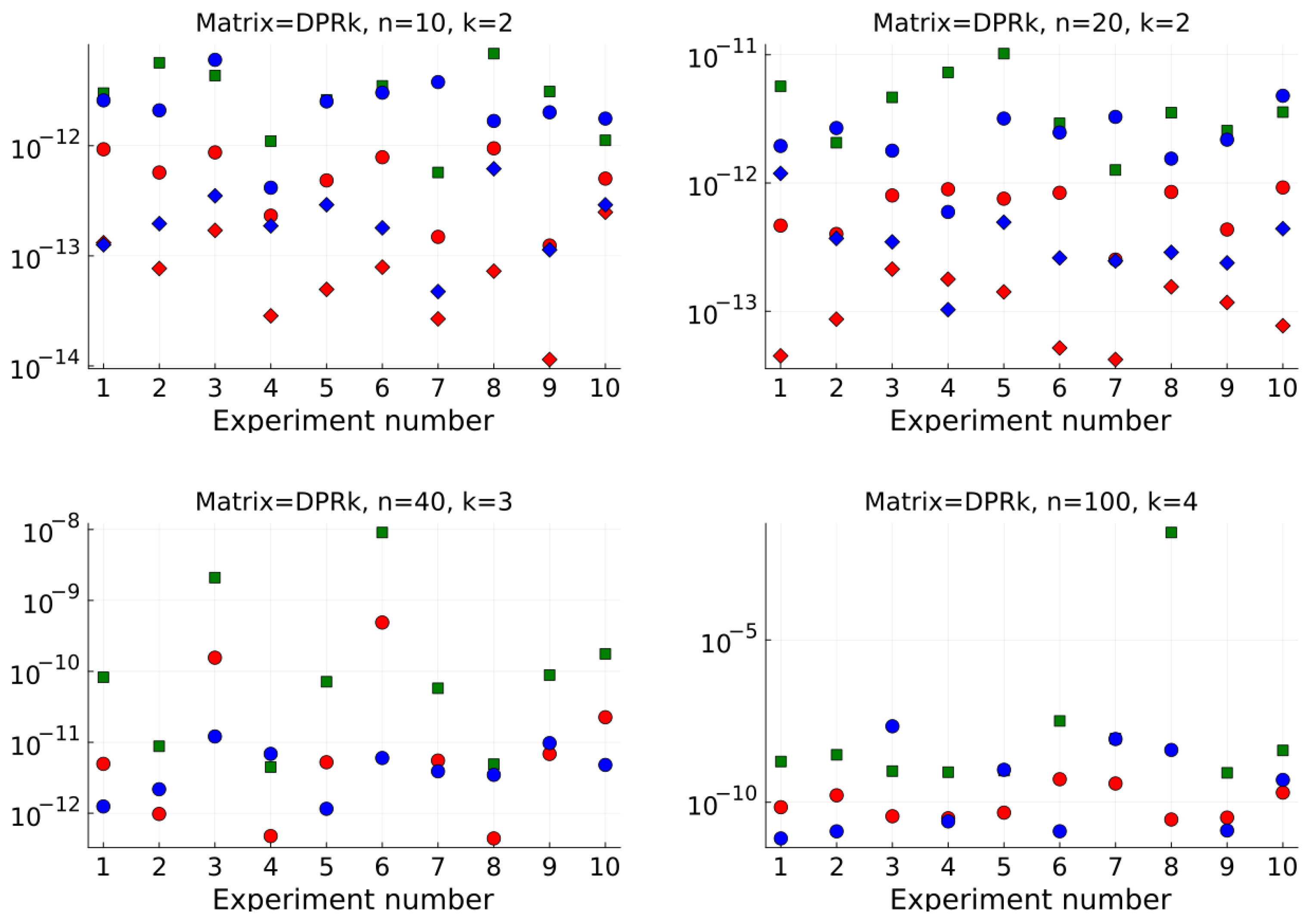
The results for DPRk matrices, displayed in Figure 2 and Table 2, are obtained by generating 10 random quaternionic DPRk matrices of each size, with  k { 2 , 3 , 4 } and we computed their eigenvalue decompositions using Algorithm 3 and Algorithm 1 for comparison. In all examples, the tolerance was set to 1 × 10 12 .

5. Discussion and Conclusions

From Figure 1 and Figure 2, we conclude that the errors approximately coincide with the tolerance and are smaller than the respective residuals, which are, in turn, smaller, but well approximated by the computed error bounds. Since the computations using BigFloat type are slow, the actual errors are computed only for the dimensions n = 10 and n = 20 . We can also conclude that residuals and error of our methods from Algorithms 2 and 3 are similar to (or even slightly smaller than) those of the quaternion QR method from Algorithm 1.
In Table 1 and Table 2, we see that the running time of our algorithms grows approximately with the square of the dimension, as expected by the O ( n 2 ) algorithm, while the running time for the quaternion QR method increases with the cube of the dimension, as expected from the general O ( n 3 ) algorithm.
The key contributions of the paper are the following:
  • Efficient algorithms for computing eigenvalue decompositions of arrow and DPRk matrices of quaternions;
  • The algorithms require O ( n 2 ) arithmetic operations, n being the order of the matrix;
  • Algorithms have proven error bounds;
  • Experiments demonstrate that the computable residual is a good estimate of actual errors;
  • Experiments demonstrate that actual errors are even smaller than predicted by the residuals;
  • In all experiments, errors and residuals are of the order of tolerance from Algorithms 2 and 3;
  • Experiments demonstrate that Rayleigh Quotient Iteration with double-shifts is efficient for non-Hermitian matrices;
  • Algorithms 2 and 3 compare favorably in terms of accuracy and speed to the quaternion QR method for general matrices from Algorithm 1.

Author Contributions

Conceptualization, N.J.S. and I.S.; formal analysis, T.C., N.J.S. and I.S.; funding acquisition, I.S.; investigation, T.C., N.J.S. and I.S.; project administration, I.S.; resources, T.C., N.J.S. and I.S.; software, T.C., N.J.S. and I.S.; writing—original draft, T.C., N.J.S. and I.S.; writing—review & editing, T.C., N.J.S. and I.S. All authors have read and agreed to the published version of the manuscript.

Funding

This work has been fully supported by the Croatian Science Foundation under project IP-2020-02-2240.

Data Availability Statement

The notebooks which contain the codes for Algorithms 2 and 3 and are used to run the experiments and make graphs and tables from Section 4 are located in the GitHub repository https://github.com/ivanslapnicar/MANAA/, accessed on 9 February 2024.

Acknowledgments

The authors wish to express their thanks to the editor and the reviewers for their succinct and valuable comments.

Conflicts of Interest

The authors declare no conflicts of interest.

References

  1. Bunse-Gerstner, A.; Byers, R.; Mehrmann, V. A quaternion QR algorithm. Numer. Math. 1989, 55, 83–95. [Google Scholar]
  2. Ahmad, S.S.; Ali, I.; Slapničar, I. Perturbation analysis of matrices over a quaternion division algebra. Electron. Trans. Numer. Anal. 2021, 54, 128–149. [Google Scholar] [CrossRef]
  3. Baker, A. Right eigenvalues for quaternionic matrices: A topological approach. Linear Algebra Appl. 1999, 286, 303–309. [Google Scholar] [CrossRef]
  4. Farenick, D.R.; Pidkowich, B.A. The spectral theorem in quaternions. Linear Algebra Appl. 2003, 371, 75–102. [Google Scholar] [CrossRef]
  5. Jia, Z.; Wang, Q.; Pang, H.K.; Zhao, M. Computing Partial Quaternion Eigenpairs with Quaternion Shift. J. Sci. Comput. 2023, 97, 41:1–41:21. [Google Scholar] [CrossRef]
  6. Lee, H.C. Eigenvalues and canonical forms of matrices with quaternion coefficients. Proc. R. Irish. Acad. 1949, 52, 253–260. [Google Scholar]
  7. De Leo, S.; Scolarici, G. Right eigenvalue equation in quaternionic quantum mechanics. J. Phys. A 2000, 33, 2971–2995. [Google Scholar]
  8. Tisseur, F.; Meerbergen, K. Quadratic eigenvalue problem. SIAM Rev. 2001, 43, 235–286. [Google Scholar] [CrossRef]
  9. Golub, G.H.; Van Loan, C.F. Matrix Computations, 4th ed.; The John Hopkins University Press: Baltimore, MD, USA, 2013. [Google Scholar]
  10. Najafi, H.S.; Edalatpanah, S.A.; Gravvanis, G.A. An efficient method for computing the inverse of arrowhead matrices. Appl. Math. Lett. 2014, 33, 1–5. [Google Scholar] [CrossRef]
  11. Jakovčević Stor, N.; Slapničar, I.; Barlow, J.L. Accurate eigenvalue decomposition of real symmetric arrowhead matrices and applications. Linear Algebra Appl. 2015, 464, 62–89. [Google Scholar] [CrossRef]
  12. Jakovčević Stor, N.; Slapničar, I.; Barlow, J.L. Forward stable eigenvalue decomposition of rank-one modifications of diagonal matrices. Linear Algebra Appl. 2015, 487, 301–315. [Google Scholar] [CrossRef]
  13. Saad, Y. Numerical Methods for Large Eigenvalue Problems; Society for Industrial and Applied Mathematics: Philadelphia, PA, USA, 2011. [Google Scholar] [CrossRef]
  14. Watkins, D.S. Unsymmetric Matrix Eigenvalue Techniques. In Handbook of Linear Algebra; Hogben, L., Ed.; CRC Press: Boca Raton, FL, USA, 2014; Chapter 56; pp. 1–12. [Google Scholar] [CrossRef]
  15. Hamilton, W.R., Sr. Lectures on Quaternions; Hodges and Smith: London, UK, 1853. [Google Scholar]
  16. Hamilton, W.R., Sr. Elements of Quaternions; Longmans, Green and Co.: London, UK, 1866. [Google Scholar]
  17. Sudbery, A. Quaternionic analysis. Math. Proc. Camb. Philos. Soc. 1979, 85, 199–225. [Google Scholar] [CrossRef]
  18. The Julia Language. Version 1.10.2. Available online: http://julialang.org/ (accessed on 9 February 2024).
  19. Quaternions.jl. Version 0.7.4. Available online: https://github.com/JuliaGeometry/Quaternions.jl (accessed on 9 February 2024).
  20. Jakovčević Stor, N.; Slapničar, I. Fast multiplication, determinants and inverses of arrowhead and diagonal-plus-rank-one matrices over associative fields. arXiv 2022, arXiv:2212.10966. [Google Scholar]
  21. Matrix Algorithms for Non-Commutative Associative Algebras. Available online: https://github.com/ivanslapnicar/MANAA/ (accessed on 9 February 2024).
  22. Joldeş, M.; Muller, J.-M. Algorithms for manipulating quaternions in floating-point arithmetic. In Proceedings of the 2020 IEEE 27th Symposium on Computer Arithmetic (ARITH), Portland, OR, USA, 7–10 June 2020; pp. 48–55. [Google Scholar] [CrossRef]
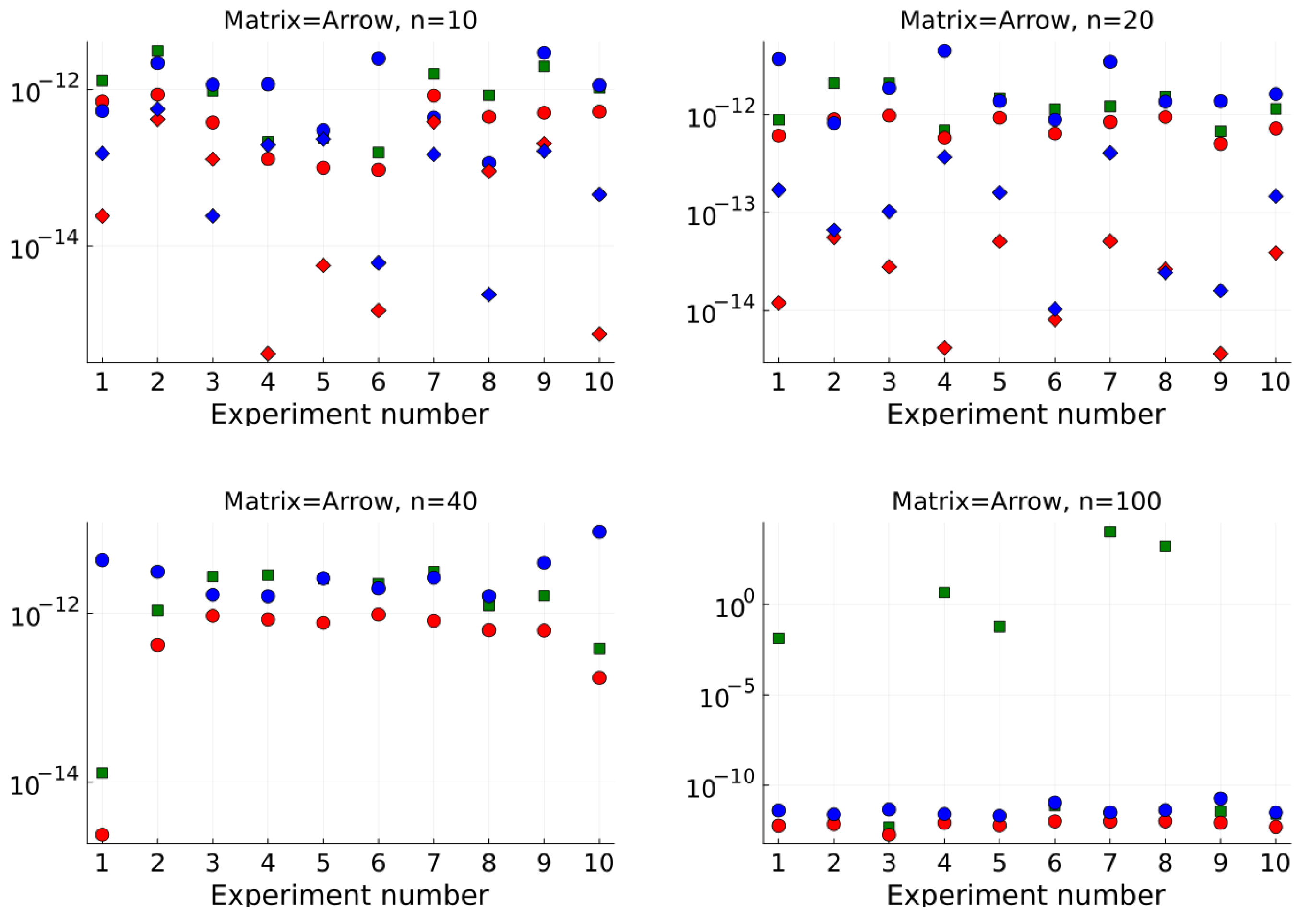
Figure 1. Error bounds (green squares), residuals and actual errors computed by Algorithm 2 (red dots and diamonds, respectively) and residuals and actual errors computed by Algorithm 1 (blue dots and diamonds, respectively). For n = 40 and n = 100 , the actual errors are not computed.
Mathematics 12 01327 g001
Figure 2. Error bounds (green squares), residuals and actual errors computed by Algorithm 2 (red dots and diamonds, respectively) and residuals and actual errors computed by Algorithm 3 (blue dots and diamonds, respectively). For n = 40 and n = 100 the actual errors are not computed.
Mathematics 12 01327 g002
Table 1. Mean number of iterations per eigenvalue and mean total running times for arrow matrices of orders n = 10 , 20 , 40 , 100 , using Algorithm 2 (RQIds) and Algorithm 1 (QR), respectively.
Mean Number of Iterations per EigenvalueMean Total Running Time (s)
nRQIdsnRQIdsQR
108100.000810.00079
209200.00260.011
4016400.0140.039
100321000.170.47
Table 2. Mean number of iterations per eigenvalue and mean total running times for DPRk matrices of orders n = 10 , 20 , 40 , 100 , using Algorithm 3 (RQIds) and Algorithm 1 (QR), respectively.
Mean Number of Iterations per EigenvalueMean Total Running Time (s)
nkRQIdsnkRQIdsQR
10271020.00180.00075
20292020.00770.011
403164030.0310.071
10042710040.250.85
Disclaimer/Publisher’s Note: The statements, opinions and data contained in all publications are solely those of the individual author(s) and contributor(s) and not of MDPI and/or the editor(s). MDPI and/or the editor(s) disclaim responsibility for any injury to people or property resulting from any ideas, methods, instructions or products referred to in the content.