Advancing Green TFP Calculation: A Novel Spatiotemporal Econometric Solow Residual Method and Its Application to China’s Urban Industrial Sectors
Abstract
1. Introduction
2. Redefining Green TFP Calculation: Innovations from the Solow Residual Method to the Spatiotemporal Econometric Solow Residual Method (STE-SRM)
2.1. Preliminary Extension of the Solow Residual Method: Incorporating Undesired Outputs
2.2. Further Extension: Defining the STE-SRM with Consideration of Three Types of Spillover Effects
3. Applying the New Method to Calculate China’s Urban Industrial Green TFPs
3.1. Configuration of the Empirical Production Function Model
3.2. Variables and Data Overview
3.3. Development of the Spatiotemporal Weight Matrix
3.4. Estimation and Model Selection for the Empirical Production Function
3.5. Calculation of China’s Urban Industrial Green TFPs Using the STE-SRM
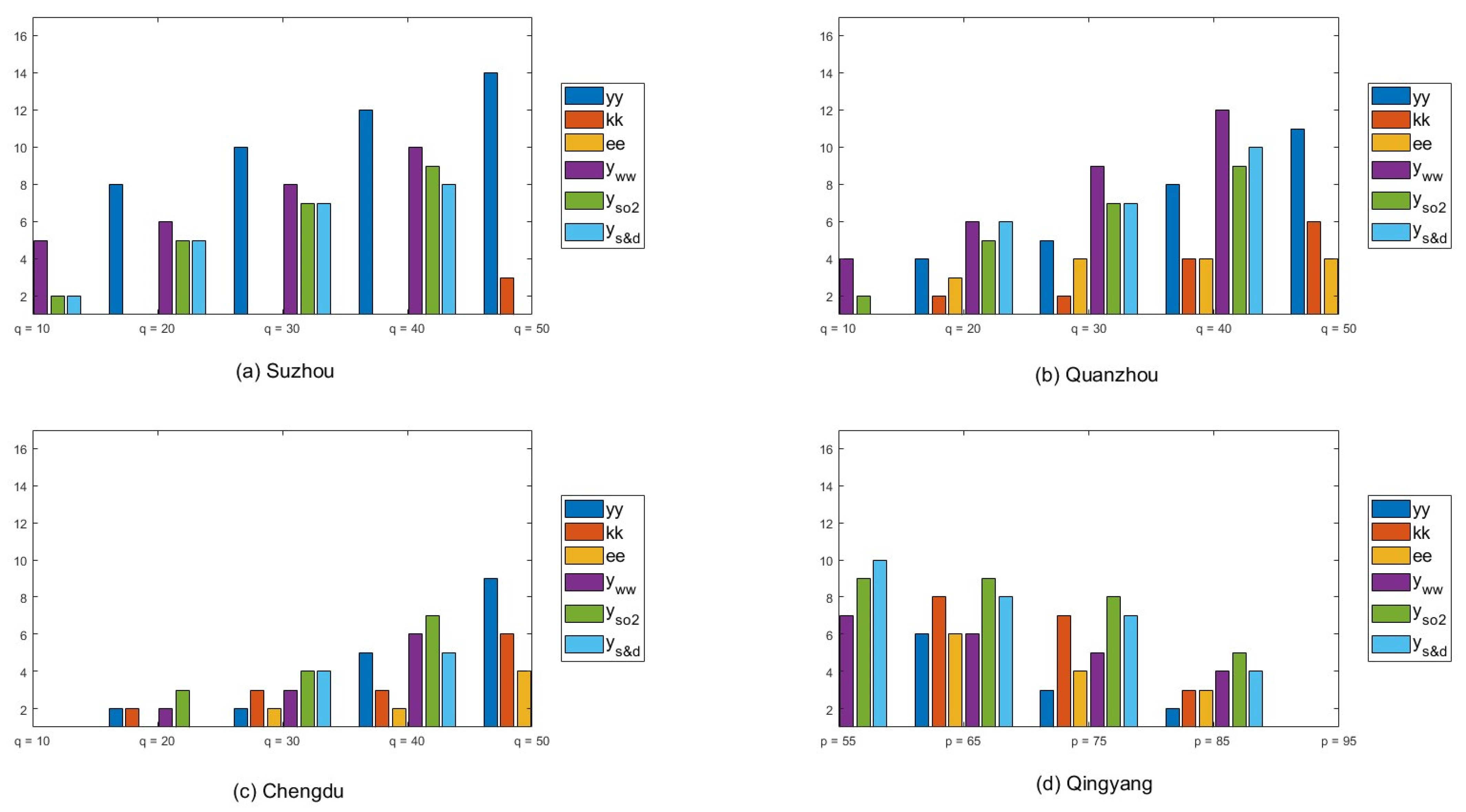
3.6. Sensitivity Analysis of the Calculated Results
4. Assessing the Accuracy of STE-SRM: Comparative Analysis with DEA-SBM and Bayesian SFA
4.1. Reassessment of China’s Urban Industrial Green TFPs Using DEA-SBM
4.2. Revised Calculation of China’s Urban Industrial Green TFPs Using Bayesian SFA
4.2.1. Fundamental Logic of Bayesian SFA in Calculating Green TFPs
4.2.2. China’s Urban Industrial Green TFPs Re-calculated by the Bayesian SFA
4.2.3. Comparative Analysis of Three Methods and Accuracy Assessment of the STE-SRM
5. Advanced Analysis of China’s Urban Industrial Green TFPs Calculated by STE-SRM: Examining Spatial Heterogeneity and Convergence
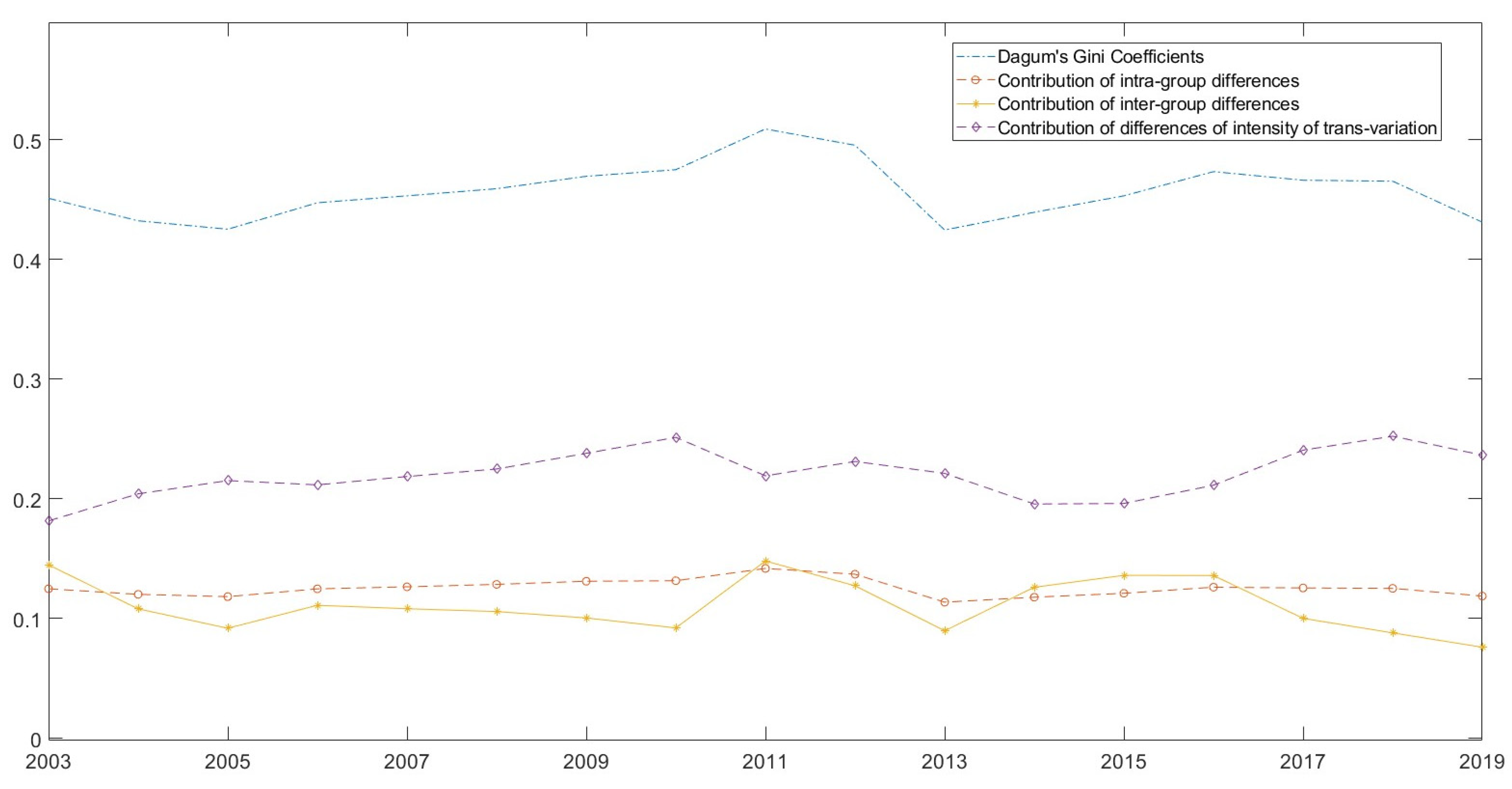
5.1. Spatial Heterogeneity Analyzed Using Dagum’s Gini Coefficient
5.2. Analyzing Spatial Convergence through Sigma and Beta Convergence Methods
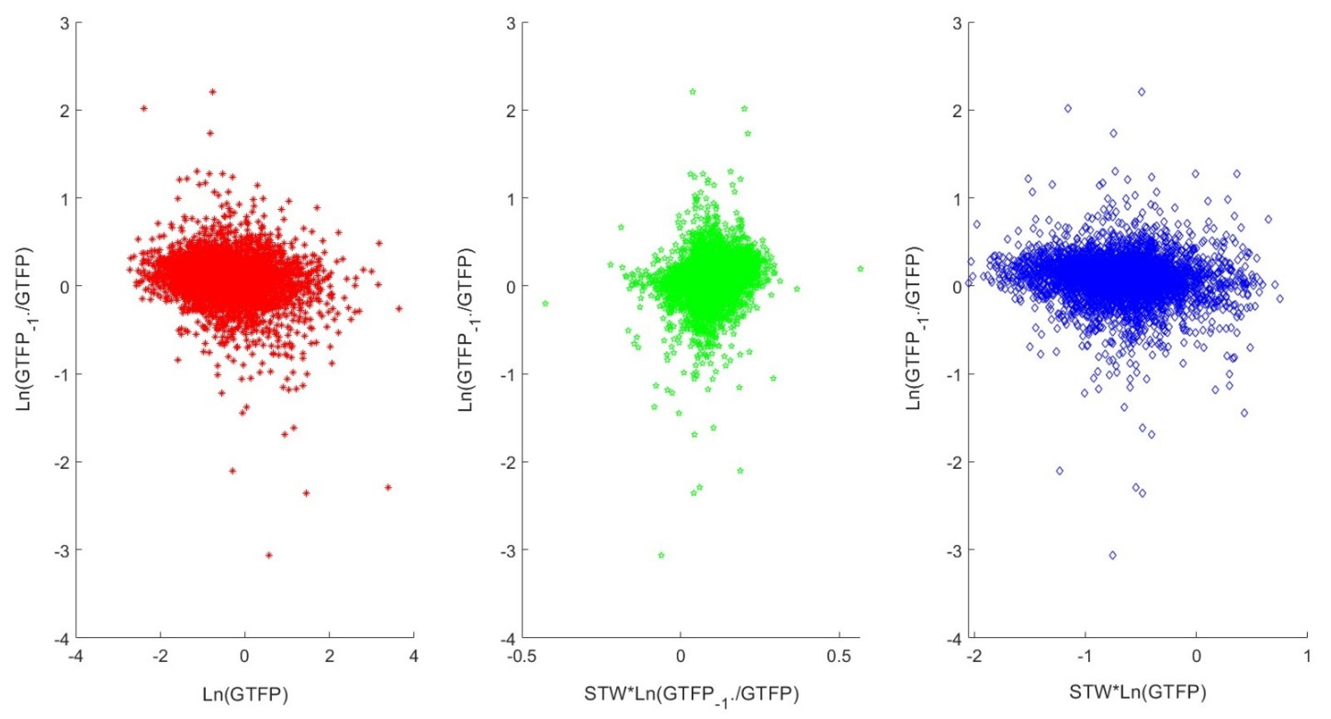
5.2.1. The Sigma Convergence and the Beta Convergence
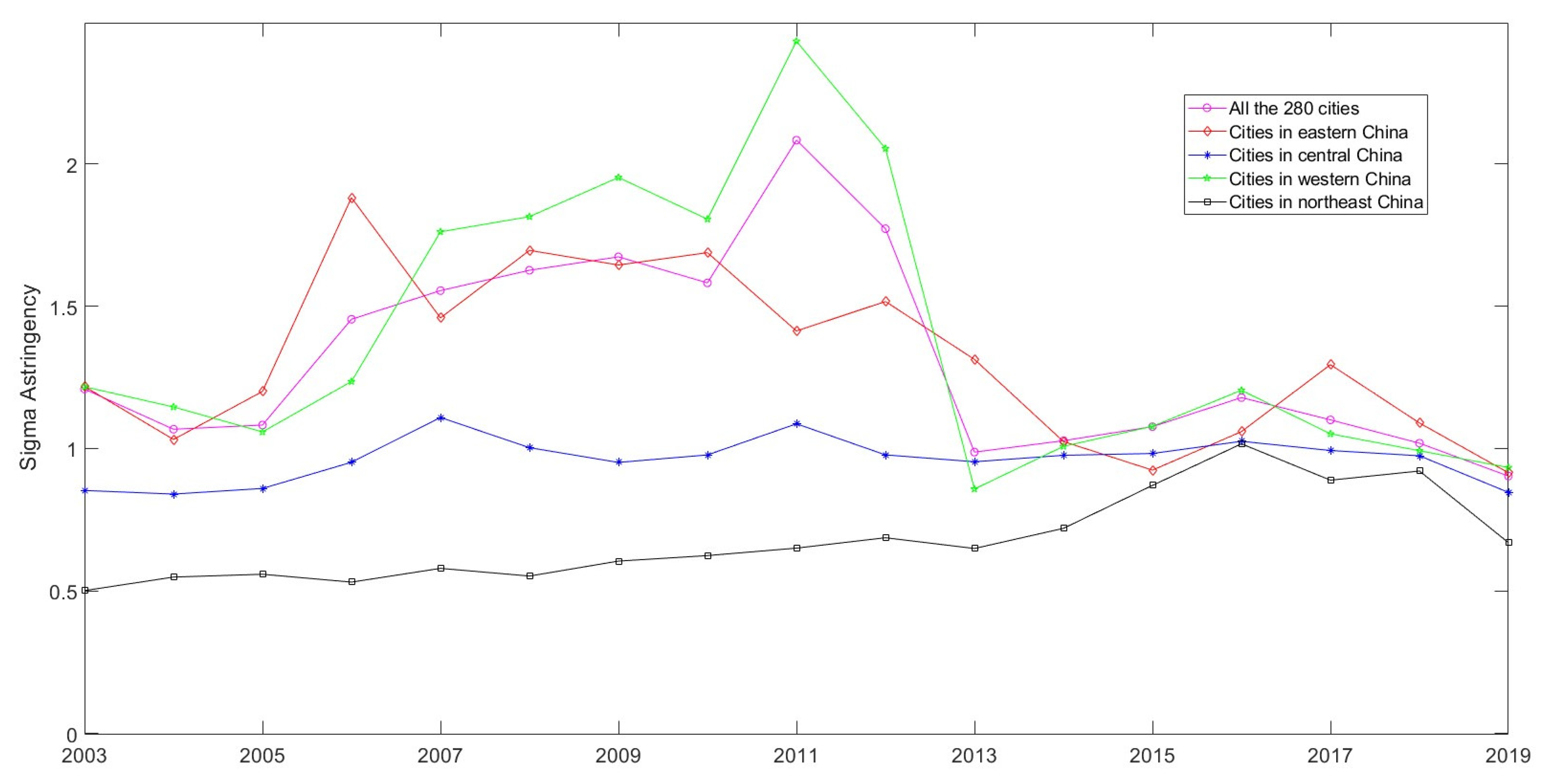
5.2.2. The Spatial Convergence Patterns of China’s Urban Industrial Green TFPs
6. Conclusions and Comments
Author Contributions
Funding
Data Availability Statement
Conflicts of Interest
References
- Chang, C.; Robin, S. Public policy, innovation and total factor productivity: An application to Taiwan’s manufacturing industry. Math. Comput. Simul. 2008, 79, 352–367. [Google Scholar] [CrossRef]
- Khanna, R.; Sharma, C. Does infrastructure stimulate total factor productivity? a dynamic heterogeneous panel analysis for Indian manufacturing industries. Q. Rev. Econ. Financ. 2021, 79, 59–73. [Google Scholar] [CrossRef]
- Kumbhakar, S.C.; Denny, M.; Fuss, M. Estimation and decomposition of productivity change when production is not efficient: A panel data approach. Econom. Rev. 2000, 19, 312–320. [Google Scholar] [CrossRef]
- Nadiri, M.I.; Prucha, I.R. Dynamic factor demand models, productivity measurement, and rates of return: Theory and an empirical application to the US Bell System. Struct. Change Econ. Dyn. 1990, 1, 263–289. [Google Scholar] [CrossRef]
- Georganta, Z. The effect of a free-market price mechanism on total factor productivity: The case of the agricultural crop industry in Greece. Int. J. Prod. Econ. 1997, 52, 55–71. [Google Scholar] [CrossRef]
- Moghaddasi, R.; Pour, A.A. Energy consumption and total factor productivity growth in Iranian agriculture. Energy Rep. 2016, 2, 218–220. [Google Scholar] [CrossRef]
- Solow, R.M. Technical change and the aggregate production function. Rev. Econ. Stat. 1957, 39, 312–320. [Google Scholar] [CrossRef]
- Tientao, A.; Legros, D.; Pichery, M.C. Technology spillover and TFP growth: A spatial Durbin model. Int. Econ. 2016, 145, 21–31. [Google Scholar] [CrossRef]
- Barilla, D.; Carlucci, F.; Cirà, A.; Ioppolo, G.; Siviero, L. Total factor logistics productivity: A spatial approach to the Italian regions. Transp. Res. Part A-Policy Pract. 2020, 136, 205–222. [Google Scholar] [CrossRef]
- Wei, W.; Fan, Q.; Guo, A. China’s Industrial TFPs at the Prefectural Level and the Law of Their Spatial–Temporal Evolution. Sustainability 2023, 15, 322. [Google Scholar] [CrossRef]
- Fang, C.; Cheng, J.; Zhu, Y.; Chen, J.; Peng, X. Green total factor productivity of extractive industries in China: An explanation from technology heterogeneity. Resour. Policy 2021, 70, 101933. [Google Scholar] [CrossRef]
- Zhu, Y.; Liang, D.; Liu, T. Can China’s underdeveloped regions catch up with green economy? A convergence analysis from the perspective of environmental total factor productivity. J. Clean. Prod. 2020, 255, 120216. [Google Scholar] [CrossRef]
- Zhong, S.; Li, J.; Chen, X.; Wen, H. A multi-hierarchy meta-frontier approach for measuring green total factor productivity: An application of pig breeding in China. Socio-Econ. Plan. Sci. 2022, 81, 101152. [Google Scholar] [CrossRef]
- Liu, S.; Lei, P.; Li, X.; Li, Y. A non-separable undesirable output modified three-stage data envelopment analysis application for evaluation of agricultural green total factor productivity in China. Sci. Total Environ. 2022, 838, 155947. [Google Scholar] [CrossRef]
- Caves, D.W.; Christensen, L.R.; Diewert, W.E. Multilateral Comparisons of Output, Input, and Productivity Using Superlative Index Numbers. Econ. J. 1982, 92, 73–86. [Google Scholar] [CrossRef]
- Färe, R.; Grosskopf, S.; Norris, M.; Zhang, Z. Productivity Growth, Technical Progress, and Efficiency Change in Industrialized Countries. Am. Econ. Rev. 1994, 84, 66–83. [Google Scholar]
- Huang, X.; Feng, C.; Qin, J.; Wang, X.; Zhang, T. Measuring China’s agricultural green total factor productivity and its drivers during 1998–2019. Sci. Total Environ. 2022, 829, 154477. [Google Scholar] [CrossRef]
- Lin, B.; Xu, M. Exploring the green total factor productivity of China’s metallurgical industry under carbon tax: A perspective on factor substitution. J. Clean. Prod. 2019, 233, 1322–1333. [Google Scholar] [CrossRef]
- Wu, J.; Xia, Q.; Li, Z. Green innovation and enterprise green total factor productivity at a micro level: A perspective of technical distance. J. Clean. Prod. 2022, 344, 131070. [Google Scholar] [CrossRef]
- Guo, B.; Yu, H.; Jin, G. Urban green total factor productivity in China: A generalized Luenberger productivity indicator and its parametric decomposition. Sust. Cities Soc. 2024, 106, 105365. [Google Scholar] [CrossRef]
- Xia, F.; Xu, J. Green total factor productivity: A re-examination of quality of growth for provinces in China. China Econ. Rev. 2020, 62, 101454. [Google Scholar] [CrossRef]
- Feng, C.; Zhong, S.; Wang, M. How can green finance promote the transformation of China’s economic growth momentum? A perspective from internal structures of green total-factor productivity. Res. Int. Bus. Financ. 2024, 70, 102356. [Google Scholar] [CrossRef]
- Tian, Y.; Feng, C. The internal-structural effects of different types of environmental regulations on China’s green total-factor productivity. Energy Econ. 2022, 113, 106246. [Google Scholar] [CrossRef]
- Jin, G.; Shen, K.; Li, J. Interjurisdiction political competition and green total factor productivity in China: An inverted-U relationship. China Econ. Rev. 2020, 61, 101224. [Google Scholar] [CrossRef]
- Battese, G.E.; Rao, D.S.P.; O’Donnell, C.J. A meta-frontier production function for estimation of technical efficiencies and technology gaps for firms operating under different technologies. J. Prod. Anal. 2004, 21, 91–103. [Google Scholar] [CrossRef]
- Arazmuradov, A.; Martini, G.; Scotti, D. Determinants of total factor productivity in former Soviet Union economies: A stochastic frontier approach. Econ. Syst. 2014, 38, 115–135. [Google Scholar] [CrossRef]
- Zhang, N.; Sun, F.; Hu, Y. Carbon emission efficiency of land use in urban agglomerations of Yangtze River Economic Belt, China: Based on three-stage SBM-DEA model. Ecol. Indic. 2024, 160, 111922. [Google Scholar] [CrossRef]
- Cheng, Z.; Jin, W. Agglomeration economy and the growth of green total-factor productivity in Chinese Industry. Socio-Econ. Plan. Sci. 2022, 83, 101003. [Google Scholar] [CrossRef]
- Song, Y.; Zhang, B.; Wang, J.; Kwek, K. The impact of climate change on China’s agricultural green total factor productivity. Technol. Forecast. Soc. Chang. 2022, 185, 122054. [Google Scholar] [CrossRef]
- Wu, H.; Ren, S.; Yan, G.; Hao, Y. Does China’s outward direct investment improve green total factor productivity in the “Belt and Road” countries? Evidence from dynamic threshold panel model analysis. J. Environ. Manag. 2020, 275, 111295. [Google Scholar] [CrossRef]
- Lesage, J.; Pace, R.K. Introduction to Spatial Econometrics; CRC Press: Boca Raton, FL, USA, 2009. [Google Scholar]
- Elhorst, J.P. Spatial Econometrics from Cross-Sectional Data to Spatial Panels; Springer: Berlin/Heidelberg, Germany, 2014. [Google Scholar]
- Zhao, Q.; Fan, Q.; Zhou, P. An Integrated Analysis of GWR Models and Spatial Econometric Global Models to Decompose the Driving Forces of the Township Consumption Development in Gansu, China. Sustainability 2022, 14, 281. [Google Scholar] [CrossRef]
- Guo, A.; Fan, Q. Calculating China’s industrial TFP at the prefectural level using spatial econometric local analysis. J. Quant. Tech. Econ. 2022, 39, 61–80. [Google Scholar]
- Hsiao, C. Analysis of Panel Data; Cambridge University Press: Cambridge, UK, 2003. [Google Scholar]
- Makieła, K. Bayesian stochastic frontier analysis of economic growth and productivity change in the EU, USA, Japan and Switzerland. Cent. Eur. J. Econom. Model. Econom. 2014, 6, 193–216. [Google Scholar]
- Makiela, K.; Ouattara, B. Foreign direct investment and economic growth: Exploring the transmission channels. Econ. Model. 2018, 72, 296–305. [Google Scholar] [CrossRef]
- Hastings, W.K. Monte Carlo sampling methods using Markov chains and their applications. Biometrika 1970, 57, 97–109. [Google Scholar] [CrossRef]
- Dagum, C. A new approach to the decomposition of the Gini income inequality ratio. Empir. Econ. 1997, 22, 515–531. [Google Scholar] [CrossRef]
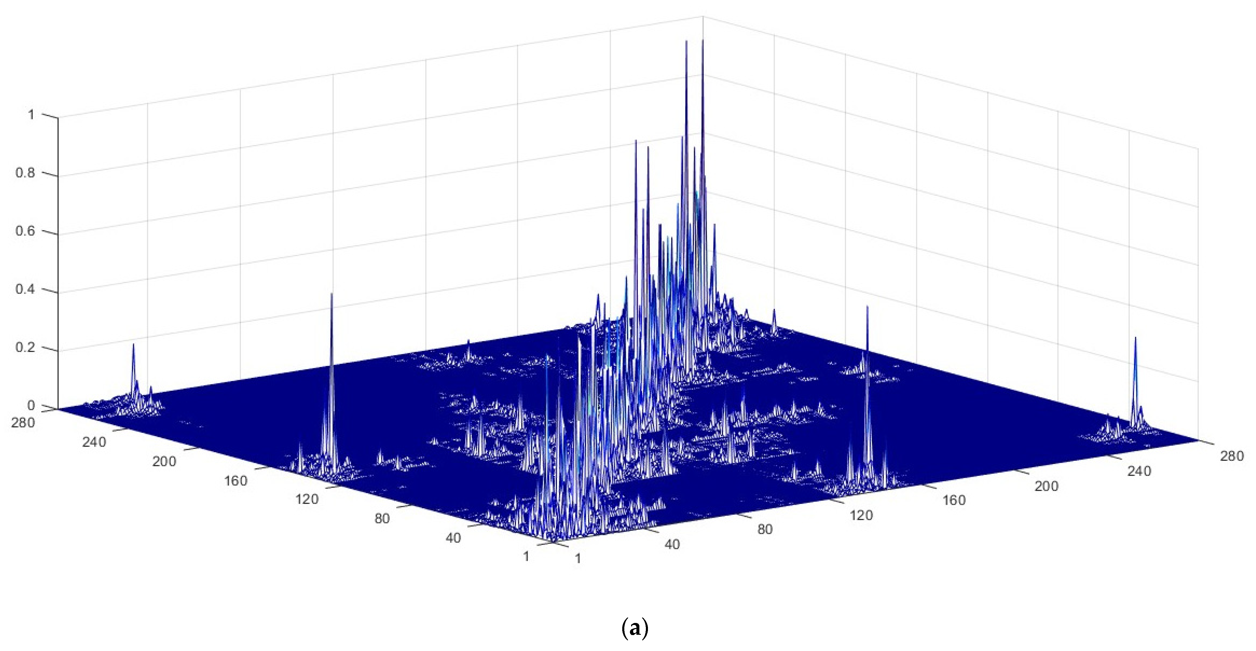
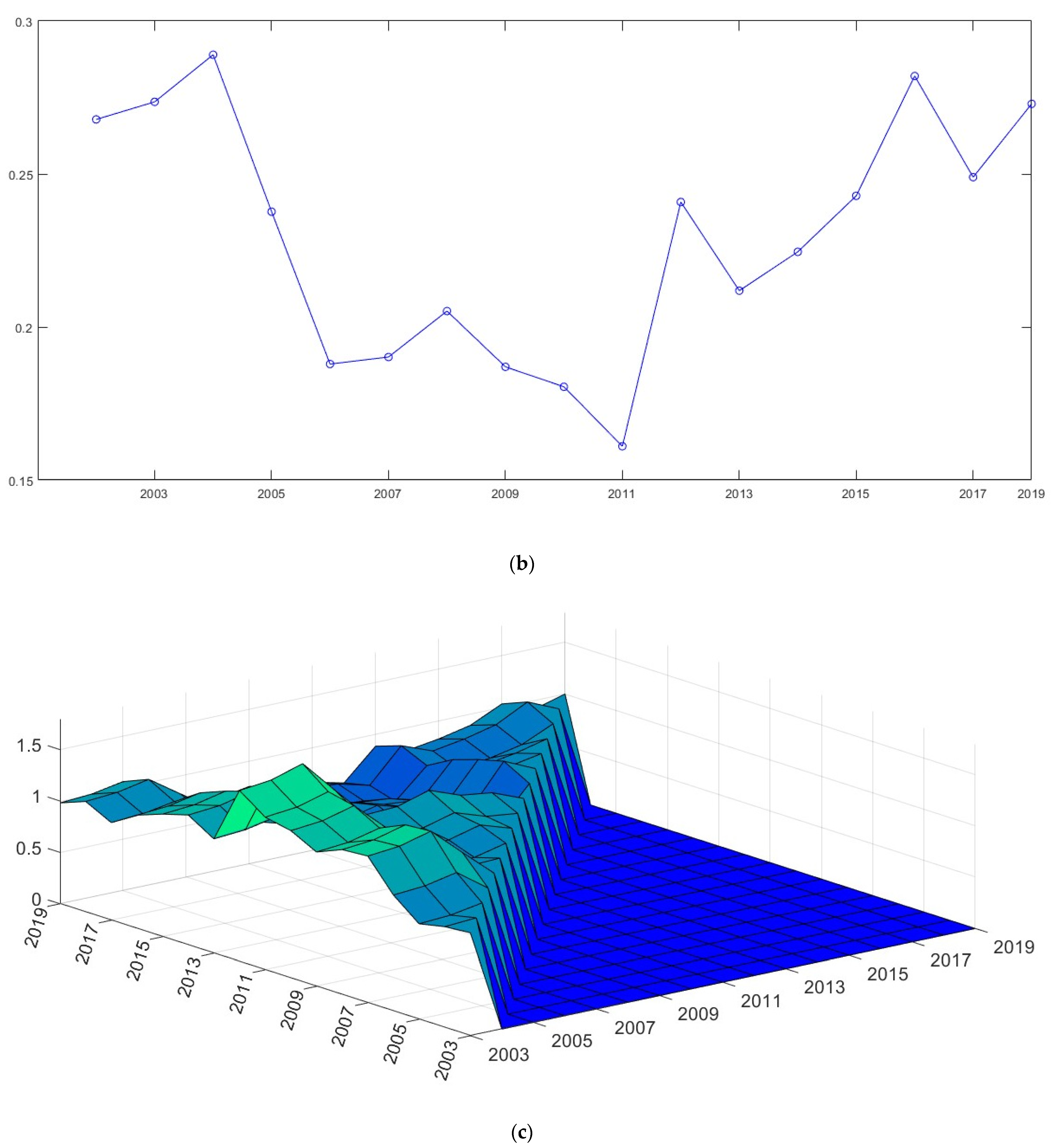
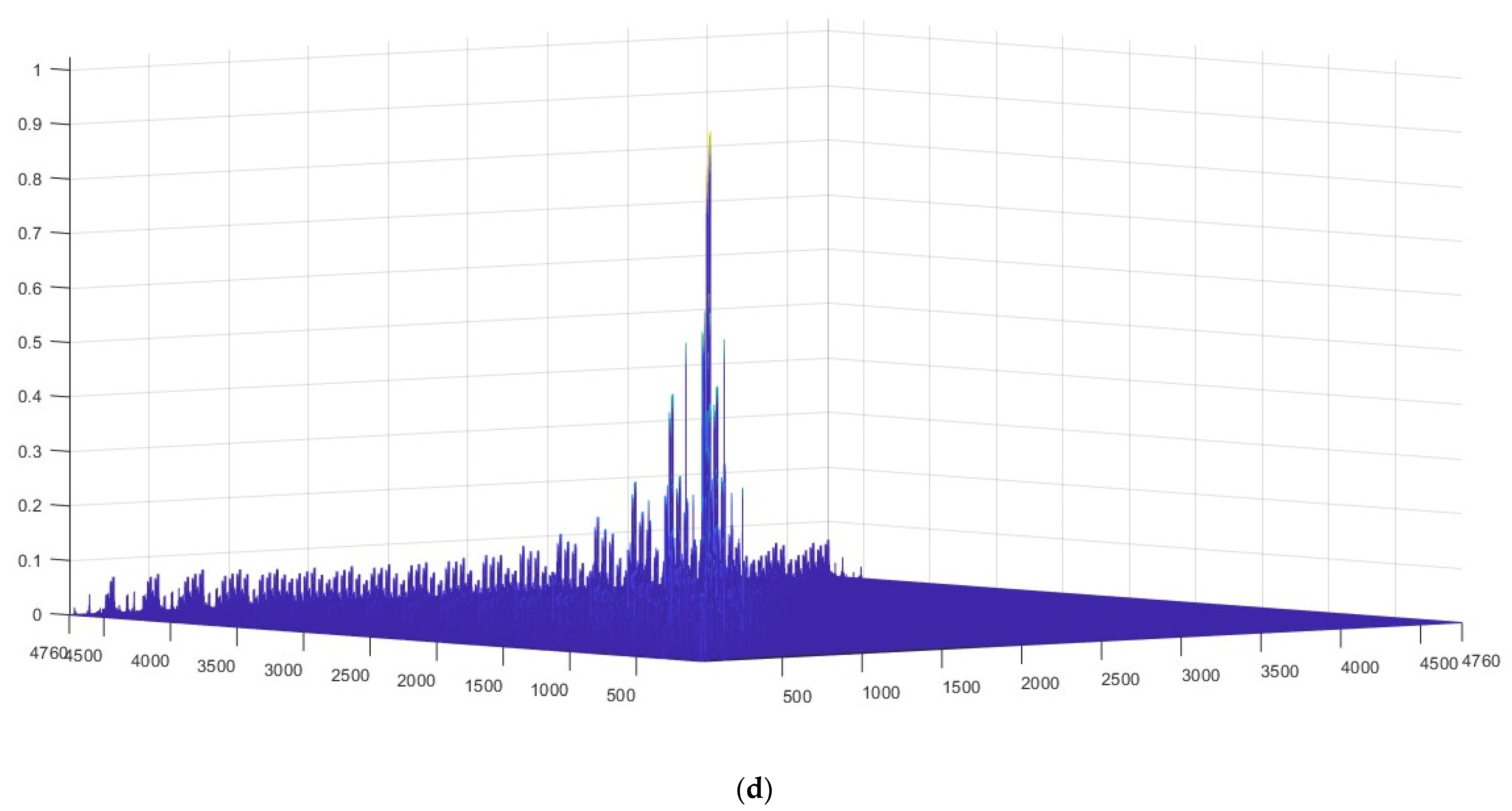
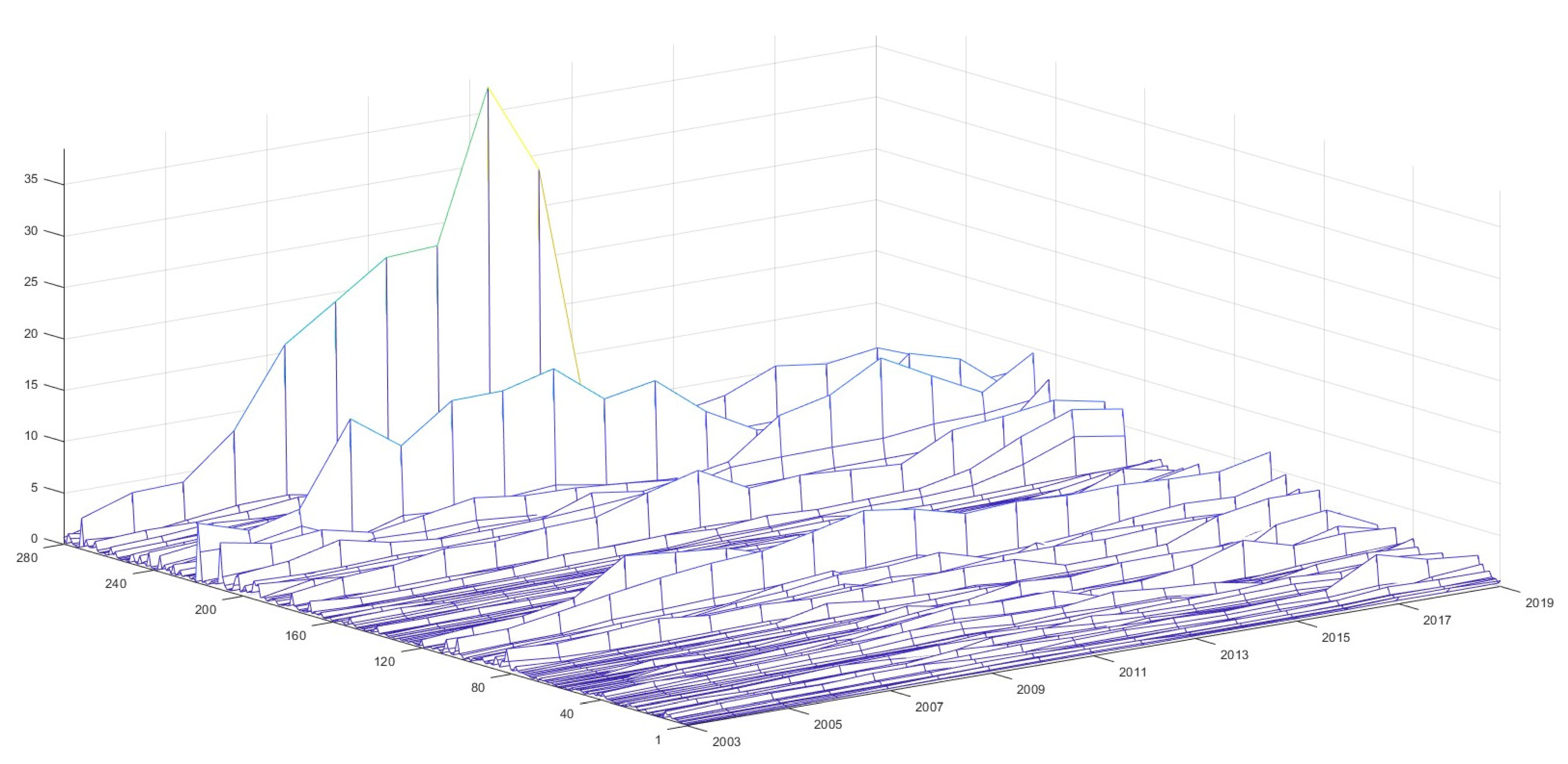



| Mean | 3.5893 | 2.4134 | -4.7971 | −5.1456 | 2.6460 | 1.8661 |
| Median | 3.6953 | 2.3427 | −4.7338 | −5.1417 | 2.6632 | 1.8044 |
| Maximum | 6.2935 | 6.9681 | −0.4706 | 3.2454 | 5.9188 | 5.9422 |
| Minimum | 0.1778 | −0.8902 | −11.6014 | −12.3200 | 0.2191 | −3.5941 |
| Std. Dev. | 0.7914 | 1.1041 | 1.4821 | 1.6388 | 0.8355 | 0.9109 |
| Skewness | −0.4191 | 0.3424 | −0.3999 | 0.0775 | 0.1042 | 0.4612 |
| Kurtosis | 3.2116 | 3.0585 | 3.4107 | 3.8777 | 2.9826 | 4.8804 |
| Jarque-Bera | 148.2233 | 93.6619 | 160.3404 | 157.5696 | 8.6778 | 870.0061 |
| Probability | 0.0000 | 0.0000 | 0.0000 | 0.0000 | 0.0131 | 0.0000 |
| Sum | 17,084.96 | 11,487.66 | −22,834.20 | −24,492.83 | 12,595.08 | 8882.55 |
| Sum Sq. Dev. | 2980.62 | 5801.75 | 10,453.91 | 12,781.42 | 3322.28 | 3948.82 |
| Observations | 4760 | 4760 | 4760 | 4760 | 4760 | 4760 |
| NSM | SXL | SAR | SEM | SDM | SDEM | SAC | GNSM | |
|---|---|---|---|---|---|---|---|---|
| Const. | 1.4267 (27.1) *** | 0.8689 (7.91) *** | 0.7545 (12.71) *** | 2.3353 (20.04) *** | 0.3893 (3.99) *** | 2.9512 (11.30) *** | 4.5441 (80.90) *** | 3.3353 (12.12) *** |
| 0.3254 (31.53) *** | 0.3864 (35.13) *** | 0.2919 (29.27) *** | 0.3612 (36.96) *** | 0.3830 (39.49) *** | 0.3699 (37.43) *** | 0.3812 (40.04) *** | 0.3691 (37.29) *** | |
| 0.2232 (26.02) *** | 0.2200 (24.87) *** | 0.1887 (22.61) *** | 0.1920 (24.16) *** | 0.1991 (25.46) *** | 0.2090 (25.43) *** | 0.1928 (24.73) *** | 0.2107 (25.66) *** | |
| −0.1042 (−12.64) *** | −0.1580 (−17.40) *** | −0.0925 (−11.73) *** | −0.1402 (−16.79) *** | −0.1456 (−18.17) *** | −0.1474 (−17.49) *** | −0.1516 (−18.78) *** | −0.1486 (−18.26) *** | |
| −0.0701 (−8.87) *** | −0.0519 (−6.29) *** | −0.0340 (−4.40) *** | −0.0260 (−3.59) *** | −0.0413 (−5.67) *** | −0.0296 (−3.99) *** | −0.0341 (−4.89) *** | −0.0297 (−4.05) *** | |
| −0.1555 (−23.73) *** | −0.1306 (−19.27) *** | −0.1138 (−17.37) *** | −0.1008 (−16.52) *** | −0.1130 (−18.85) *** | −0.1211 (−19.53) *** | −0.1057 (−17.80) *** | −0.1242 (−20.10) *** | |
| −0.2647 (−10.16) *** | −0.5436 (−22.56) *** | −0.2732 (−8.01) *** | −0.2158 (−4.98) *** | |||||
| 0.1106 (5.36) *** | −0.1152 (−6.02) *** | 0.1230 (4.93) *** | 0.1544 (5.65) *** | |||||
| 0.1696 (9.09) *** | 0.1881 (11.43) *** | 0.0784 (2.51) ** | 0.0398 (1.38) | |||||
| 0.0369 (1.54) | 0.1702 (7.96) *** | 0.2359 (9.77) *** | 0.2204 (9.09) *** | |||||
| −0.1773 (−11.16) *** | −0.0097 (−0.66) | −0.1866 (−8.36) *** | −0.2097 (−9.50) *** | |||||
| 0.3780 (21.27) *** | 0.9010 (38.57) *** | −0.3050 (−89.77) *** | −0.2000 (−2.80) *** | |||||
| 0.8860 (49.16) *** | 0.9120 (85.53) *** | 0.9400 (184.88) *** | 0.9000 (74.52) *** | |||||
| 0.7101 | 0.7308 | 0.6928 | 0.7785 | −0.4350 | 0.7909 | 0.7849 | 0.7918 | |
| 0.1816 | 0.1686 | 0.1653 | 0.1386 | 0.1311 | 0.1307 | 0.1346 | 0.1301 | |
| −2690.40 | −2511.90 | −830.05 | −430.42 | −328.35 | −293.62 | −403.77 | −1932.70 |
| SAR | SEM | SDEM | |||||||
|---|---|---|---|---|---|---|---|---|---|
| Individual Fixed | Period Fixed | Both Fixed | Individual Fixed | Period Fixed | Both Fixed | Individual Fixed | Period Fixed | Both Fixed | |
| Const. | 0.0775 (21.17) *** | −0.0117 (−2.19) ** | −1.3077 (−24.98) *** | 0.2537 (7.90) *** | −0.2291 (−4.63) *** | −1.6788 (−100.74) *** | 0.0643 (1.80) * | −0.2107 (−4.18) *** | −1.6166 (−74.71) *** |
| 0.4159 (39.18) *** | 0.3643 (37.74) *** | 0.5454 (53.53) *** | 0.4329 (41.42) *** | 0.4108 (43.12) *** | 0.5508 (77.17) *** | 0.4841 (44.26) *** | 0.4057 (41.74) *** | 0.5468 (54.21) *** | |
| 0.1918 (20.29) *** | 0.1924 (24.98) *** | 0.1345 (16.99) *** | 0.1643 (18.14) *** | 0.1943 (26.01) *** | 0.1313 (16.65) *** | 0.1712 (19.98) *** | 0.2054 (25.89) *** | 0.1326 (16.80) *** | |
| −0.1986 (−23.47) *** | −0.1036 (−14.06) *** | −0.1725 (−24.17) *** | −0.1788 (−21.90) *** | −0.1437 (−18.67) *** | −0.1722 (−30.79) *** | −0.1907 (−24.29) *** | −0.1390 (−17.86) *** | −0.1720 (−24.93) *** | |
| 0.0633 (9.08) *** | −0.1139 (−15.28) *** | −0.0670 (−10.21) *** | 0.0432 (6.42) *** | −0.0886 (−12.50) *** | −0.0665 (−11.01) *** | −0.0100 (−1.45) | −0.0844 (−11.33) *** | −0.0667 (−10.28) *** | |
| −0.0932 (−14.43) *** | −0.0869 (−14.49) *** | −0.0581 (−10.71) *** | −0.0816 (−13.18) *** | −0.0902 (−15.87) *** | −0.0596 (−11.44) *** | −0.0851 (−14.43) *** | −0.0993 (−16.57) *** | −0.0589 (−10.91) *** | |
| −0.4753 (−12.45) *** | −0.0360 (−1.04) | −0.0318 (−1.00) | |||||||
| 0.3861 (10.46) *** | 0.1056 (4.39) *** | 0.1172 (3.54) *** | |||||||
| 0.0074 (0.23) | 0.0020 (0.07) | −0.0367 (−2.16) ** | |||||||
| 0.3875 (13.05) *** | 0.0404 (1.67) * | 0.0108 (0.47) | |||||||
| −0.2241 (−7.90) *** | −0.1131 (−5.35) *** | −0.0152 (−0.61) | |||||||
| 0.1620 (66.49) *** | 0.3850 (22.94) *** | 0.1070 (53.95) *** | |||||||
| 0.7230 (35.54) *** | 0.8730 (50.53) *** | 0.3310 (87.89) *** | 0.7520 (42.41) *** | 0.8740 (43.91) *** | 0.3100 (45.23) | ||||
| 0.8032 | 0.5725 | 0.6043 | 0.8277 | 0.6805 | 0.6096 | 0.8464 | 0.6836 | 0.6105 | |
| 0.0702 | 0.1339 | 0.0449 | 0.0639 | 0.1180 | 0.0446 | 0.0569 | 0.1167 | 0.0444 | |
| 1217.00 | −328.64 | 2281.40 | 1426.10 | −45.60 | 2295.00 | 1700.40 | −19.45 | 2303.40 | |
| C-D | CD-T | CD-Linear-T | Trans-Log | Trans-Log-T | |
|---|---|---|---|---|---|
| 0.6462 (57.82) *** | 0.5184 (40.24) *** | −0.0383 (−16.75) *** | −0.1203 (−10.96) *** | −0.0997 (−9.29) *** | |
| 0.3437 (26.83) *** | 0.4055 (32.11) *** | 0.0133 (5.48) *** | 0.0408 (2.09) ** | 0.0221 (1.17) | |
| 0.1136 (10.57) *** | 0.0676 (6.34) *** | 0.0014 (0.68) | 0.0431 (3.15) *** | 0.0139 (1.03) | |
| −0.1846 (−19.07) *** | −0.2218 (−23.37) *** | −0.0076 (−4.08) *** | −0.0618 (−4.58) *** | −0.0606 (−4.66) *** | |
| −0.0314 (−3.34) *** | 0.0246 (2.62) *** | −0.0085 (−4.66) *** | −0.0058 (−0.44) | 0.0147 (1.14) | |
| −0.0999 (−12.19) *** | −0.0824 (−10.43) *** | 0.0076 (4.74) *** | 0.0377 (3.35) *** | 0.0220 (2.01) ** | |
| −0.4806 (−6.25) *** | −0.0417 (−18.23) *** | −0.1344 (−9.89) *** | −0.9893 (−9.28) *** | −0.8297 (−8.06) *** | |
| −0.0457 (−3.62) *** | −0.0271 (−2.17) ** | ||||
| 0.0776 (4.86) *** | 0.0722 (4.64) *** | ||||
| 0.0145 (0.87) | 0.0119 (0.72) | ||||
| 0.0202 (1.35) | 0.0277 (1.92) ** | ||||
| 0.0435 (3.45) *** | 0.0401 (3.27) *** | ||||
| 0.1826 (1.46) | 0.2570 (2.10) ** | ||||
| −0.0406 (−6.17) *** | −0.0277 (−4.26) *** | ||||
| −0.0215 (−1.62) | −0.0221 (−1.73) * | ||||
| −0.0479 (−4.18) *** | −0.0281 (−2.51) ** | ||||
| 0.0421 (3.72) *** | 0.0345 (3.11) *** | ||||
| 0.0543 (0.59) | 0.0723 (0.82) | ||||
| 0.0536 (6.78) *** | −0.0534 (−6.82) *** | ||||
| −0.0881 (−7.71) *** | −0.0843 (−7.51) *** | ||||
| 0.0116 (1.18) | 0.0150 (1.57) | ||||
| 0.6164 (5.78) *** | 0.6585 (6.23) *** | ||||
| 0.0300 (5.22) *** | 0.0257 (4.61) *** | ||||
| −0.0244 (−2.92) *** | −0.0190 (−2.32) *** | ||||
| −0.4508 (−5.54) *** | −0.5236 (−6.59) *** | ||||
| −0.0109 (−3.02) *** | −0.0059 (−1.67) * | ||||
| 0.2608 (3.66) *** | 0.1262 (1.81) * | ||||
| −1.1460 (−2.73) *** | 0.0396 (16.15) *** | ||||
| 0.3842 (5.33) *** | 0.8187 (37.88) *** | −1.2758 (−3.09) *** | |||
| 0.3084 (12.09) *** | |||||
| 0.0655 (3.41) *** | |||||
| −0.1572 (−8.62) *** | |||||
| 0.0553 (3.02) *** | |||||
| −0.1244 (−8.58) *** | |||||
| 0.2432 (1.83) * | |||||
| 0.3458 (12.94) *** | 0.3176 (13.59) *** | 0.2923 (13.94) *** | 0.3070 (12.38) *** | 0.2876 (12.29) *** | |
| 0.3562 (29.69) *** | 0.3475 (32.51) *** | 0.3307 (33.35) *** | 0.3460 (29.81) *** | 0.3387 (30.54) *** | |
| MDD | −1050.55 | −975.72 | −862.52 | −1024.41 | −967.64 |
| SSE | 322.88 | 311.53 | 280.00 | 310.59 | 300.14 |
| STE-SRM | Bayesian SFA | DEA-SBM | |
|---|---|---|---|
| Mean | 0.9872 | 0.6628 | 0.4640 |
| Median | 0.6260 | 0.6933 | 0.4308 |
| Maximum | 38.2525 | 0.9407 | 1.0000 |
| Minimum | 0.0663 | 0.1533 | 0.0021 |
| Std. Dev. | 1.4340 | 0.1404 | 0.2250 |
| Coefficient of Variation | 0.6884 | 4.7208 | 2.0622 |
| 75th Quartile | 1.0893 | 0.7698 | 0.5769 |
| 25th Quartile | 0.3729 | 0.5768 | 0.3080 |
| Quartile Deviation | 0.7163 | 0.1931 | 0.2689 |
| NSM | SXL | SAR | SEM | SDM | SDEM | SAC | GNSM | ||
|---|---|---|---|---|---|---|---|---|---|
| Const. | 0.0473 (10.94) *** | 0.0356 (4.78) *** | 0.0032 (0.76) | 0.0301 (2.91) *** | 0.0127 (1.74) * | 0.0122 (0.85) | 0.0150 (2.13) ** | 0.0077 (0.56) | |
| −0.0539 (−11.59) *** | −0.0495 (−9.57) *** | −0.0505 (−11.04) *** | −0.0562 (−11.14) *** | −0.0545 (−10.70) *** | −0.0571 (−10.01) *** | −0.0544 (−11.11) *** | −0.0555 (−10.95) *** | ||
| −0.0204 (−1.93) * | 0.0188 (1.81) * | −0.0414 (−2.07) ** | −0.0146 (−0.69) | ||||||
| 0.4850 (121.70) *** | 0.4990 (123.63) *** | 0.3250 (6.87) *** | 0.3000 (1.25) | ||||||
| 0.6180 (12.10) *** | 0.6640 (5.24) *** | 0.3510 (6.84) *** | 0.5250 (2.79) *** | ||||||
| 0.0289 | 0.0295 | 0.0279 | 0.0619 | 0.0281 | 0.0642 | 0.0634 | 0.0657 | ||
| 0.0646 | 0.0646 | 0.0627 | 0.0624 | 0.0626 | 0.0622 | 0.0623 | 0.0621 | ||
| −220.52 | −218.65 | 1384.1 | 1397.52 | 1385.64 | 1401.32 | 1397.56 | −144.6 | ||
| the Beta astringency coefficients | Total effects | −0.0539 | −0.0699 | −0.0981 | −0.0713 | −0.0562 | −0.0985 | −0.0806 | −0.1001 |
| Direct effects | −0.0539 | −0.0495 | −0.0507 | −0.0546 | −0.0562 | −0.0571 | −0.0545 | −0.0556 | |
| Indirect effects | 0.0000 | −0.0204 | −0.0474 | −0.0167 | 0.0000 | −0.0414 | −0.0261 | −0.0445 | |
| NSM | SXL | SAR | SEM | SDM | SDEM | SAC | GNSM | |||
|---|---|---|---|---|---|---|---|---|---|---|
| Cities in Eastern China | −0.0349 (−4.25) *** | −0.0314 (−3.61) *** | −0.0333 (−4.15) *** | −0.0403 (−4.69) *** | −0.0394 (−4.64) *** | −0.0397 (−4.51) *** | −0.0386 (−4.55) *** | −0.0405 (−4.68) *** | ||
| −0.0227 (−1.22) | 0.0405 (2.24) ** | 0.0104 (0.38) | 0.0378 (1.10) | |||||||
| 0.5090 (73.48) *** | 0.5709 (78.99) *** | 0.3220 (3.80) *** | 0.4759 (0.51) | |||||||
| 0.0127 | 0.0131 | 0.0135 | 0.0639 | 0.0015 | 0.0631 | 0.0648 | 0.0687 | |||
| 75.88 | 76.63 | 560.34 | 567.41 | 562.35 | 567.49 | 565.94 | 111.71 | |||
| the Beta astringency coefficients | Total effects | −0.0349 | −0.0541 | −0.0678 | −0.0403 | 0.0026 | −0.0293 | −0.0569 | −0.0052 | |
| Direct effects | −0.0349 | −0.0314 | −0.0334 | −0.0403 | −0.0392 | −0.0397 | −0.0387 | −0.0404 | ||
| Indirect effects | 0.0000 | −0.0227 | −0.0344 | 0.0000 | 0.0418 | 0.0104 | −0.0183 | 0.0352 | ||
| Cities in Central China | −0.0424 (−5.23) *** | −0.0462 (−4.92) *** | −0.0406 (−5.04) *** | −0.0455 (−5.21) *** | −0.0507 (−5.43) *** | −0.0487 (−5.31) *** | −0.0428 (−5.11) *** | −0.0510 (−5.44) *** | ||
| 0.0152 (0.80) | 0.0423 (2.18) ** | 0.0230 (1.07) | 0.0461 (1.58) | |||||||
| 0.2010 (62.52) *** | 0.2500 (5.38) *** | 0.1340 (50.94) *** | 0.2691 (0.37) | |||||||
| 0.0202 | 0.0199 | 0.0188 | 0.0352 | 0.0196 | 0.0353 | 0.0350 | 0.0386 | |||
| 74.65 | 74.98 | 523.69 | 527.42 | 525.90 | 527.99 | 525.98 | 86.62 | |||
| the Beta astringency coefficients | Total effects | −0.0424 | −0.0310 | −0.0508 | −0.0455 | −0.0112 | −0.0257 | −0.0494 | −0.0067 | |
| Direct effects | −0.0424 | −0.0462 | −0.0406 | −0.0455 | −0.0506 | −0.0487 | −0.0428 | −0.0509 | ||
| Indirect effects | 0.0000 | 0.0152 | −0.0102 | 0.0000 | 0.0394 | 0.0230 | −0.0066 | 0.0442 | ||
| Cities in Western China | −0.0721 (−8.14) *** | −0.0701 (−7.22) *** | −0.0707 (−8.03) *** | −0.0748 (−7.95) *** | −0.0722 (−7.48) *** | −0.0740 (−7.74) *** | −0.0730 (−8.02) *** | −0.0729 (−7.24) *** | ||
| −0.0103 (−0.50) | 0.0081 (0.39) | −0.0320 (−1.33) | −0.0117 (−0.14) | |||||||
| 0.3270 (4.18) *** | 0.3320 (4.13) *** | 0.2220 (48.59) *** | 0.2000 (0.20) | |||||||
| 0.0469 | 0.0464 | 0.0450 | 0.0603 | 0.0446 | 0.0614 | 0.0600 | 0.0605 | |||
| −233.83 | −233.71 | 232.10 | 233.65 | 232.16 | 234.56 | 233.47 | −225.28 | |||
| the Beta astringency coefficients | Total effects | −0.0721 | −0.0804 | −0.1051 | −0.0748 | −0.0960 | −0.1060 | −0.0938 | −0.1058 | |
| Direct effects | −0.0721 | −0.0701 | −0.0708 | −0.0748 | −0.0723 | −0.0740 | −0.0731 | −0.0730 | ||
| Indirect effects | 0.0000 | −0.0103 | −0.0342 | 0.0000 | −0.0237 | −0.0320 | −0.0208 | −0.0328 | ||
| Cities in Northeast China | −0.0934 (−5.92) *** | −0.0803 (−4.88) *** | −0.0880 (−5.61) *** | −0.0850 (−5.06) *** | −0.0795 (−4.87) *** | −0.0860 (−5.24) *** | −0.0869 (−5.47) *** | −0.0842 (−4.72) *** | ||
| −0.0841 (−2.64) *** | −0.0624 (−1.94) * | −0.1295 (−3.12) *** | −0.1176 (−1.73) * | |||||||
| 0.3290 (3.34) *** | 0.2540 (2.95) *** | 0.2869 (3.13) *** | 0.0716 (0.17) | |||||||
| 0.0590 | 0.0693 | 0.0658 | 0.0704 | 0.0662 | 0.0878 | 0.0770 | 0.0871 | |||
| −60.74 | −57.25 | 131.55 | 130.32 | 133.30 | 135.29 | 131.73 | −53.19 | |||
| the Beta astringency coefficients | Total effects | −0.0934 | −0.1644 | −0.1311 | −0.0850 | −0.1902 | −0.2155 | −0.1219 | −0.2174 | |
| Direct effects | −0.0934 | −0.0803 | −0.0882 | −0.0850 | −0.0800 | −0.0860 | −0.0871 | −0.0844 | ||
| Indirect effects | 0.0000 | −0.0841 | −0.0429 | 0.0000 | −0.1102 | −0.1295 | −0.0348 | −0.1330 | ||
Disclaimer/Publisher’s Note: The statements, opinions and data contained in all publications are solely those of the individual author(s) and contributor(s) and not of MDPI and/or the editor(s). MDPI and/or the editor(s) disclaim responsibility for any injury to people or property resulting from any ideas, methods, instructions or products referred to in the content. |
© 2024 by the authors. Licensee MDPI, Basel, Switzerland. This article is an open access article distributed under the terms and conditions of the Creative Commons Attribution (CC BY) license (https://creativecommons.org/licenses/by/4.0/).
Share and Cite
Xiang, X.; Fan, Q. Advancing Green TFP Calculation: A Novel Spatiotemporal Econometric Solow Residual Method and Its Application to China’s Urban Industrial Sectors. Mathematics 2024, 12, 1365. https://doi.org/10.3390/math12091365
Xiang X, Fan Q. Advancing Green TFP Calculation: A Novel Spatiotemporal Econometric Solow Residual Method and Its Application to China’s Urban Industrial Sectors. Mathematics. 2024; 12(9):1365. https://doi.org/10.3390/math12091365
Chicago/Turabian StyleXiang, Xiao, and Qiao Fan. 2024. "Advancing Green TFP Calculation: A Novel Spatiotemporal Econometric Solow Residual Method and Its Application to China’s Urban Industrial Sectors" Mathematics 12, no. 9: 1365. https://doi.org/10.3390/math12091365
APA StyleXiang, X., & Fan, Q. (2024). Advancing Green TFP Calculation: A Novel Spatiotemporal Econometric Solow Residual Method and Its Application to China’s Urban Industrial Sectors. Mathematics, 12(9), 1365. https://doi.org/10.3390/math12091365


