Synchronization in a Three Level Network of All-to-All Periodically Forced Hodgkin–Huxley Reaction–Diffusion Equations

Abstract

This article focuses on the analysis of dynamics emerging in a network of Hodgkin–Huxley reaction–diffusion equations. The network has three levels. The three neurons in level 1 receive a periodic input but do not receive inputs from other neurons. The three neurons in level 2 receive inputs from one specific neuron in level 1 and all neurons in level 3. The neurons in level 3 (all other neurons) receive inputs from all other neurons in levels 2 and 3. Furthermore, the right-hand side of pre-synaptic neurons is connected to the left-hand side of the post-synaptic neurons. The synchronization phenomenon is observed for neurons in level 3, even though the system is initiated with different functions. As far as we know, it is the first time that evidence of the synchronization phenomenon is provided for spatially extended Hodgkin–Huxley equations, which are periodically forced at three different sites and embedded in such a hierarchical network with space-dependent coupling interactions.

1. Introduction

The main objective of this article is to provide some insights about the qualitative analysis of a non-autonomous neuronal network of Hodgkin–Huxley (HH) reaction–diffusion (RD) equations. The model under consideration writes as follows:

$$\left\{\begin{array}{cc}\hfill V_{it}& ={\overline{g}}_{Na}{m}_i^3{h}_i\left(E_{Na}-V_i\right)+{\overline{g}}_K{n}_i^4\left(E_K-V_i\right)+{\overline{g}}_L\left(E_L-V_i\right)+V_{ixx}\hfill \\ \hfill & +H_i(V_1,\dots ,V_N)+I_i(x,t),i\in \{1,\dots ,N\}\hfill \\ \hfill n_{it}& ={\alpha }_n\left(V_i\right)(1-n_i)-{\beta }_n\left(V_i\right)n_i\hfill \\ \hfill m_{it}& ={\alpha }_m\left(V_i\right)(1-m_i)-{\beta }_m\left(V_i\right)m_i\hfill \\ \hfill h_{it}& ={\alpha }_h\left(V_i\right)(1-h_i)-{\beta }_h\left(V_i\right)h_i\hfill \end{array}\right.$$

(1)

The dynamics of each individual neuron are described by a standard HH equation containing ionic (sodium, potassium, leakage) fluxes and a spatial diffusion term. As a reminder, in this setting, V stands for the voltage between the exterior and the interior of the cell, and $n,m,h$ stand for the gating variables. We refer, for example, to [1,2,3] and the references therein for details about the HH-RD systems. The functions and parameters on the above equation are as follows:

$$\begin{array}{cccc}\hfill {\alpha }_n\left(V\right)& =0.01\frac{-V-55}{exp(-5.5-0.1V)-1},\hfill & \hfill {\beta }_n\left(V\right)& =0.125\frac{exp(-(V+65\left)\right)}{80},\hfill \\ \hfill {\alpha }_m\left(V\right)& =0.1\frac{-V-40}{exp(-4-0.1V)-1},\hfill & \hfill {\beta }_m\left(V\right)& =4\frac{exp(-(V+65\left)\right)}{18},\hfill \\ \hfill {\alpha }_h\left(V\right)& =0.07\frac{exp(-(V+65\left)\right)}{20},\hfill & \hfill {\beta }_h\left(V\right)& =\frac{1}{1+exp(-0.1V-3.5)}.\hfill \end{array}$$

These values correspond to the ones found in [3]. We recall that the HH equations are of the voltage-gated type: when the values of m, n, and h are close to 1, the corresponding ionic fluxes conductances are close to their maximal values. On the opposite, if they are close to zero, there is almost no ionic currents flowing trough the membrane. One of the most important contributions of the Hodgkin and Huxley was to fit the $\alpha$ and $\beta$ functions with the available data thanks to the voltage clamp technique. We refer to the original paper [4] and, for example, to the textbooks [2,5] for more details. As for the space domain, we consider a one-dimensional interval $\Omega =(a,b)$. We assume Neumann boundary conditions. Each neuron is embedded in a network and receives inputs from its pre-synaptic neurons trough the coupling term

$$H_i(V_1,\dots ,V_N)=\sum _{j=0}^N{c}_{ji}\left(x\right)(S-V_i)\Gamma \left(V_j(b-x)\right),$$

(2)

with,

$$\Gamma \left(V\right)=\frac{1}{1+e^{-\lambda (V-\theta )}},\lambda =20,\theta =10.$$

These type of coupling functions have been used, for example, in [6,7] in the context of the Hindmarsh–Rose ODE networks. It was later used in [3] in the networks of HH PDEs. Since $\Gamma \left(V\right)$ is a sigmoid function, the pre-synaptic neurons $V_j$ of $V_i$ will have an effect only when they spike. The parameter S is set to

$$S=100,$$

which means that when there is enough pre-synaptic activity, the neuron $V_i$ will tend to S; this corresponds to depolarization and, eventually, a spike. This means that in our network, all neurons have an excitatory effect. As we deal with spatial extended neurons, we need to specify where the connectivity arises with respect to the spatial position. We assume that the neurons are connected from the right-hand side of the pre-synaptic neuron j to the left-hand side of the post-synaptic neuron i. This is to model the fact that action potential travels through the axon in one direction, and kicks the post-synaptic neuron through synaptic connections. As a consequence, the function c, which stands for the coupling strength, is generally set to zero everywhere except in the left-hand part of size l, $(a,a+l)$ of the neuron. We assume that c has the following expression:

$$c_{ij}\left(x\right)=\left\{\begin{array}{cc}c& \forall x\in (a,a+l),\hfill \\ 0& \forall x otherwise,\hfill \end{array}\right.$$

and we use the term $V_j(b-x)$ to express that only the right-hand side of the pre-synaptic neuron j connects to the left-hand side of the neuron i. Finally, the network topology is set as follows. We assume that there are three levels in the network that separate the network into three sets of neurons. At level 1, the set one contains three neurons that receive periodic input $I_{i_0}\left(t\right),I_{i_1}\left(t\right),I_{i_2}\left(t\right)$. Each of these three neurons possesses only one unidirectional connection to a unique neuron in level 2. Therefore, the second set of neurons also contains three neurons, each of which receives an input from a single neuron in level 1. The neurons in this second set connect to all the neurons in levels 2 and 3. Finally, the last set of neurons, which correspond to level 3, are connected to all of the neurons of levels 2 and 3, but do not receive any inputs from the neurons in level 1. The network topology is represented in Figure 1.

Finally, the functions $I(x,t)$ are set to 0 for all but the three neurons in the set 1. For these three neurons, indexed by $\{i_0,i_1,i_2\}$, a periodic signal is injected at neuron’s left-hand as follows:

$$I_{i_0}(x,t)=Acos\left(at\right),I_{i_1}(x,t)=Acos(at+b),I_{i_2}=-I_{i_0}-I_{i_1}.$$

for $x<a+l$ for some small l and 0 elsewhere. The dynamics of the $HH$ ODE have been widely studied. For the parameters’ values considered here, it is known from numerical studies that the HH system undergoes a subcritical Hopf bifurcation. For a certain region around $I\simeq 7$, we can observe the coexistence of a stable limit cycle and a stable stationary point. In the next section, we will consider a non-autonomous HH ODE system.

The present article is a theoretical and numerical investigation of Equation (1), a mathematical model that arises in a neuroscience context. Aside from the standard HH framework, several specificities of the model, namely, periodic stimulation at three different locations with specific frequencies, are indeed inspired by recent studies that are worth mentioning here. The topic of brain dynamics modeling has attracted an increasing interest, in particular, for the therapeutically potential of non-invasive brain stimulation (NIBS), see, for example, reference [8] for a summary about the transcranial alternating current stimulation (tACS) method, its mechanisms, use for cognitive applications, and novel developments for personalized stimulation. A software, SimNIBS, (current version 4) has been developed to simulate NIBS on realistic domains representing brain geometries, see [9]. SimNIBS is based on the finite element method to solve time-dependent Poisson equations. In the context of EEG data-driven modeling, recent studies have shown the importance of periodic current sources to retrieve real spatiotemporal signals, see [10,11]. HH neural networks have also been used recently to model the effect of specific frequency stimulation to help patients suffering from post-traumatic stress disorder (PTSD), see [12].

The remaining part of this article is dived as follows: in Section 2, we provide a numerical description of the effect of the variation in the frequency of the periodic input in a single HH equation. In Section 3, we provide a theoretical mathematical framework for a description of the solutions of Equation (1) as well as theoretical insights about the synchronization phenomenon. Section 4 is devoted to the numerical simulations of Equation (1) and the illustrations of the synchronization phenomenon. Finally, we conclude in Section 5.

2. Forced ODE HH Equations

The aim of this section is to provide some insights about the response of a single HH ODE when the frequency of a periodic stimulus $I\left(t\right)$ is varied. We consider a single HH non-autonomous equation as follows:

$$\left\{\begin{array}{cc}\hfill V_t& ={\overline{g}}_{Na}{m}^{3}h\left(E_{Na}-V\right)+{\overline{g}}_K{n}^4\left(E_K-V\right)+{\overline{g}}_L\left(E_L-V\right)+I\left(t\right),\hfill \\ \hfill n_t& ={\alpha }_n\left(V\right)(1-n)-{\beta }_n\left(V\right)n,\hfill \\ \hfill m_t& ={\alpha }_m\left(V\right)(1-m)-{\beta }_m\left(V\right)m,\hfill \\ \hfill h_t& ={\alpha }_h\left(V\right)(1-h)-{\beta }_h\left(V\right)h,\hfill \end{array}\right.$$

(3)

with $I\left(t\right)$ set to:

$$I\left(t\right)=Acos\left(at\right),$$

with $A=7$ and $a\in (0,2)$. The outputs of the simulations are reported in Figure 2, Figure 3 and Figure 4. A careful analysis of the numerical simulations lead to the following observations:

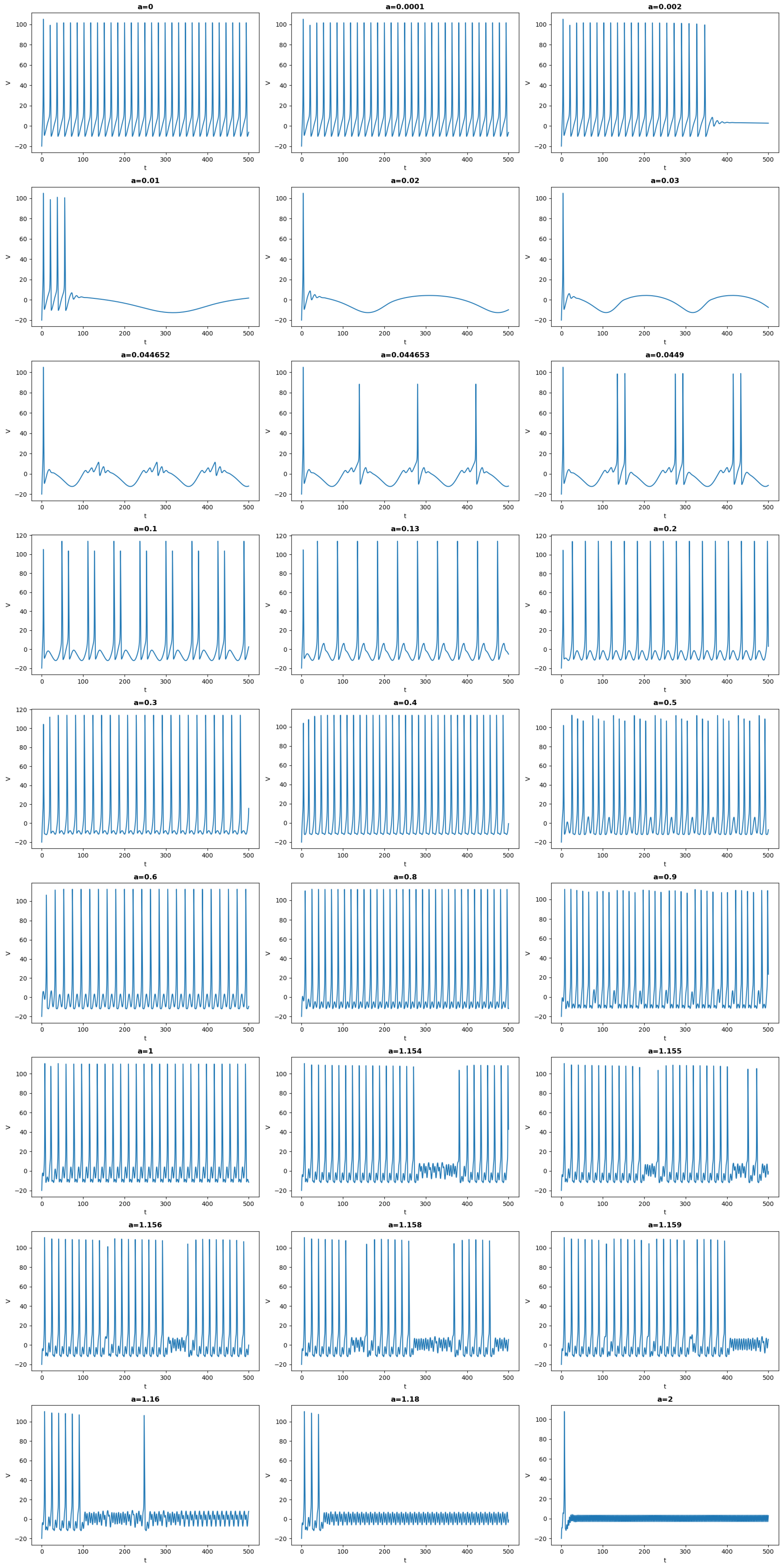
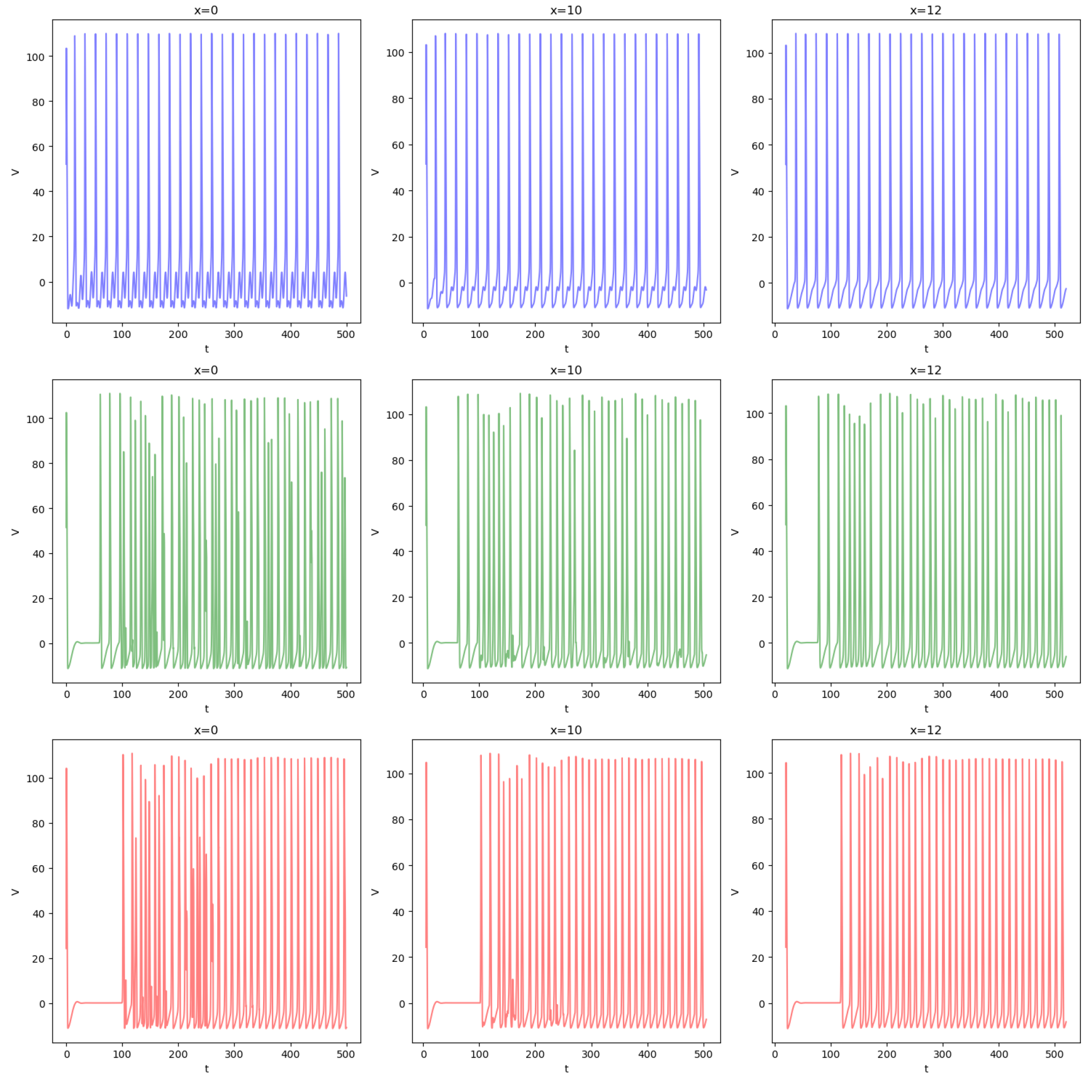
• When the frequency of the input is very slow ($a=0.0001$), then the behavior is akin to an autonomous HH with $I=7$. For the initial conditions considered here, the system evolves toward a limit cycle and the frequency observed is intrinsic to the autonomous HH;
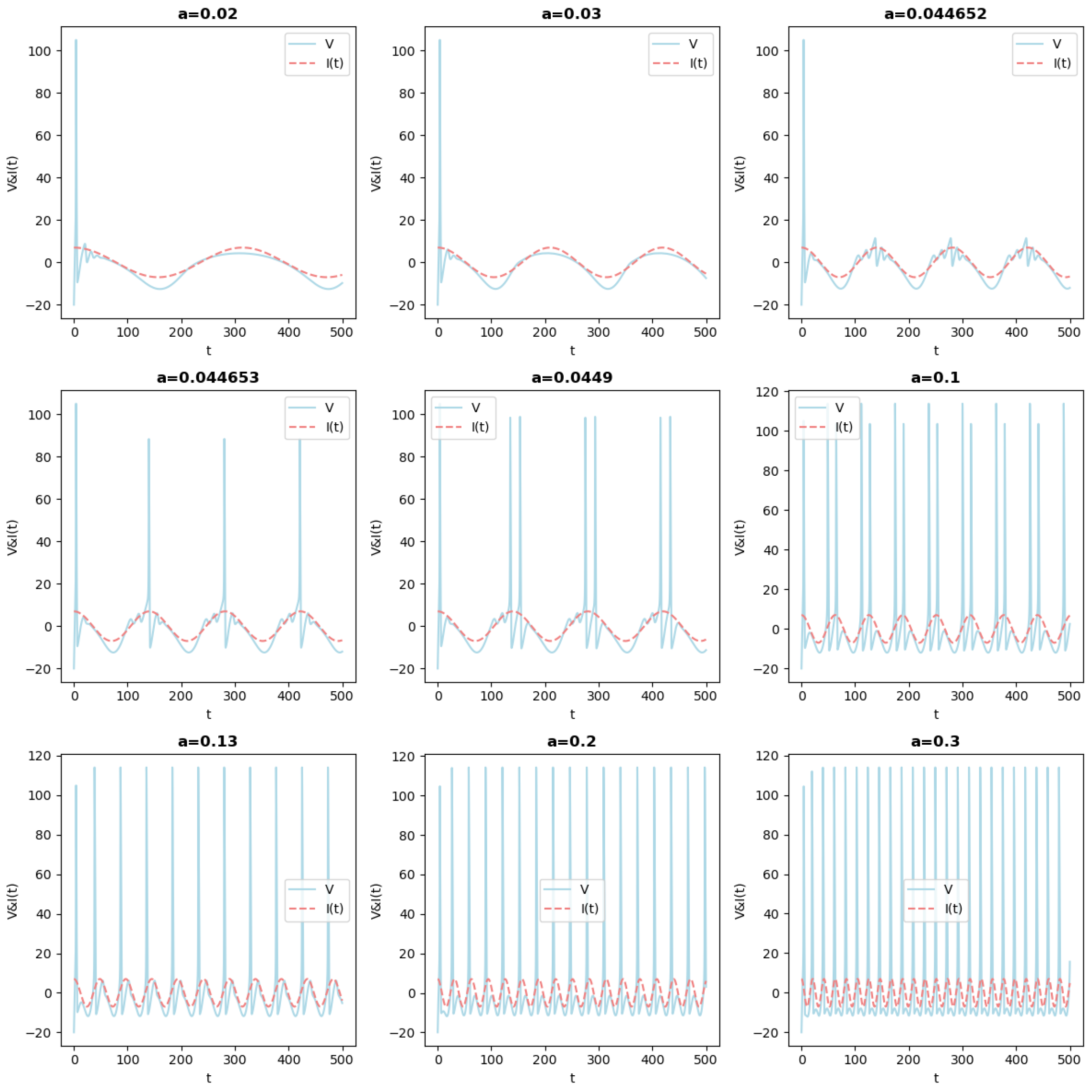
• When the frequency increases, for a range of $a\in (0.01,0.4)$, there are two frequencies that play a role. There is a recurrent pattern with a frequency of $\frac{a}{2\pi }$, which is imposed by $I\left(t\right)$, i.e., the time-periodicity of the global recurrent pattern is given by the periodicity of $I\left(t\right)$. Concurrently, within this period, the dynamics of HH appear. For example, for $a=0.03$, the system stays at an equilibrium that varies with $I\left(t\right)$, but there is no spike. For other values, such as $a\in (0.04465,0.3)$ some spikes arise. For some values, one can observe the appearance of the so-called mixed-mode oscillations (MMOs), see, for example, references [13,14,15,16,17,18] and the references therein cited;
• It is worth emphasizing the qualitative difference between the output for $a=0.0001$ and $a=0.4$. Although the oscillatory frequency is the same, for $a=0.0001$, the oscillations correspond to the intrinsic frequency of the non-autonomous HH. In this case, one can clearly observe the characteristic difference of the trajectories in a slow manifold and a jump, see [19] and the references therein cited. For $a=0.4$, however, the frequency is imposed by $I\left(t\right)$;
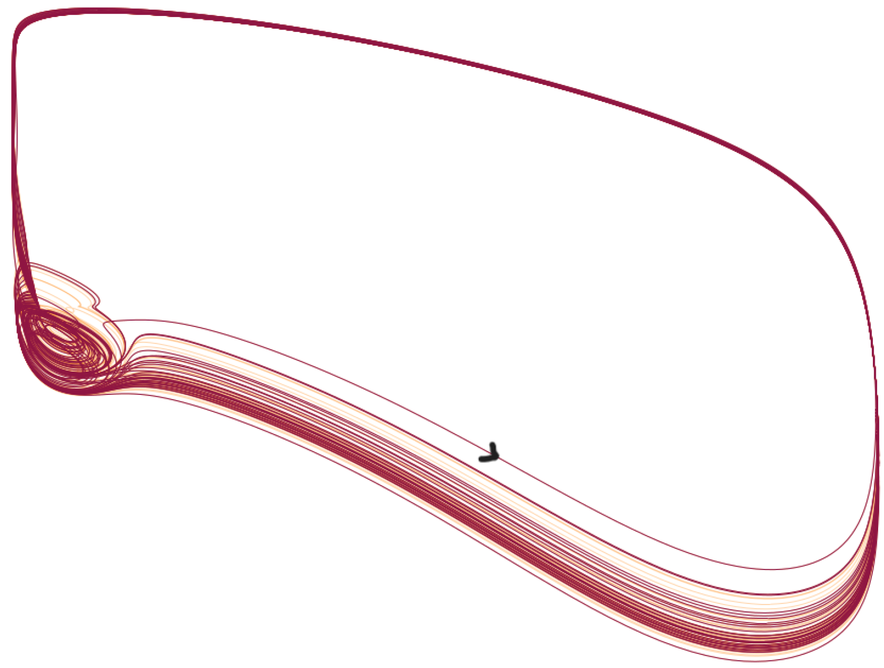
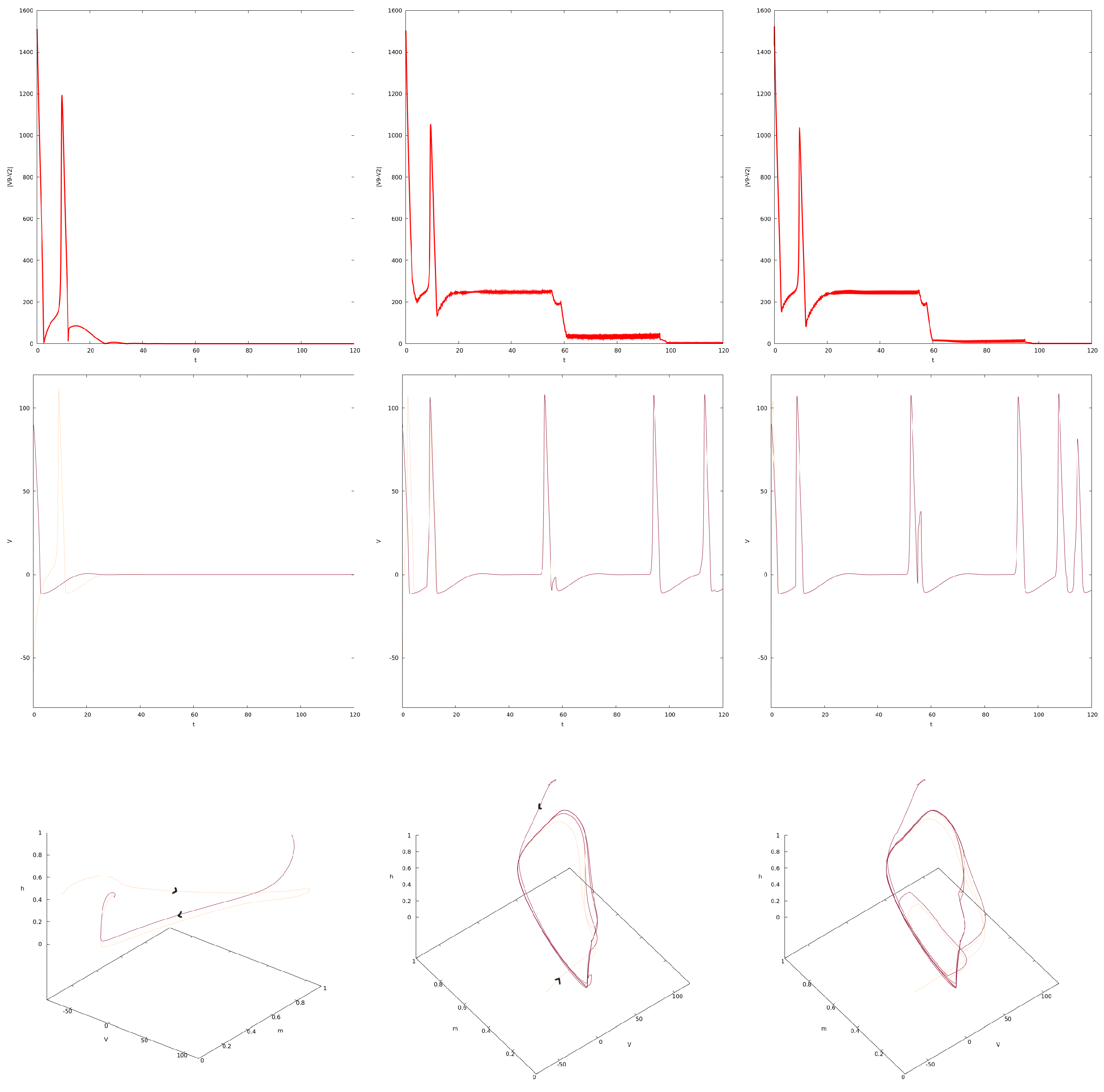
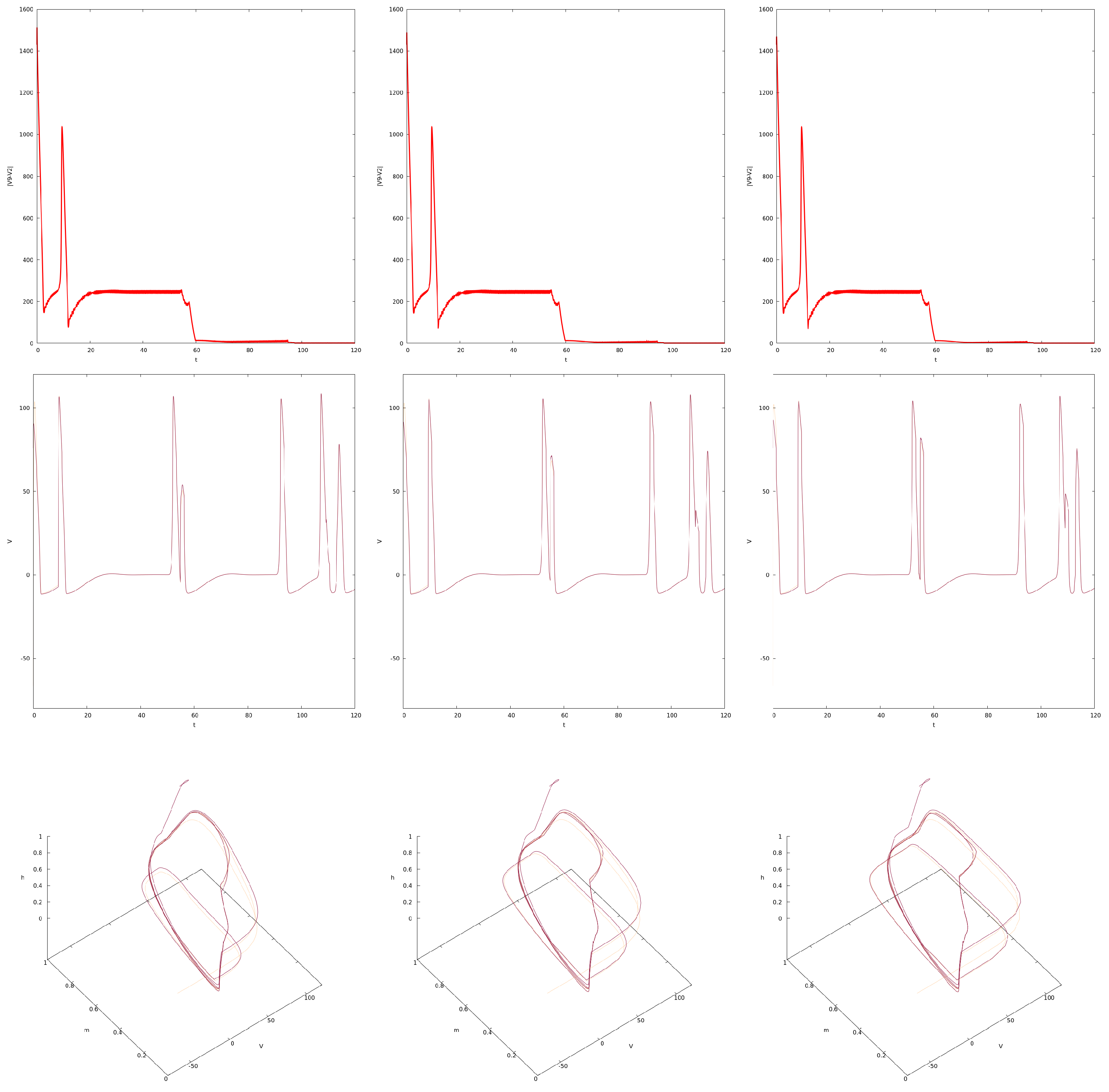
• After $a=0.5$, the situation changes, and the period of $I\left(t\right)$ becomes smaller than the one of the output, i.e., there is a periodic pattern, but its period results from a not straightforward interplay between the drive $I\left(t\right)$ and the dynamics of HH. An analysis of such an interplay was carried out in [20] in the simpler case of a FitzHugh–Nagumo system that was kicked periodically. For some values of the frequency, the behavior is more complicated and difficult to predict. The neuron can, in this case, spike or not in an erratic way. This is the case, for example, for a = 1.156. See also Figure 4, in which the solution is represented in the $(V,m,h)$ phase space. In this case, the behavior is difficult to predict: the trajectories can switch between small and large oscillations in an unpredictable manner. This picture illustrates a geometry appearing in some slow–fast systems, in which the switching between the small and large oscillations occurs as canard solutions and in a tiny space region. We refer to [16,21] for such systems derivated from the FitzHugh–Nagumo system and with three time scales. Although there is no small parameter in the HH equation, its hidden slow–fast nature has been studied for a long time, see [5,22,23];
• When the frequency is too high, for example, for $a=2$, only small oscillations persist.

Figure 2. Simulations of Equation (3). This figure illustrates the potential V as a function of time as the parameter a is increased from 0 to 2 with a current injection $I\left(t\right)=7cos\left(at\right)$.

Figure 2. Simulations of Equation (3). This figure illustrates the potential V as a function of time as the parameter a is increased from 0 to 2 with a current injection $I\left(t\right)=7cos\left(at\right)$.

Figure 3. Simulations of Equation (3). This figure illustrates the potential V as a function of time as the parameter a is increased from $0.02$ to $0.3$ along with the injected current $I\left(t\right)=7cos\left(at\right)$. It emphasizes how the injected current imposes its frequency.

Figure 3. Simulations of Equation (3). This figure illustrates the potential V as a function of time as the parameter a is increased from $0.02$ to $0.3$ along with the injected current $I\left(t\right)=7cos\left(at\right)$. It emphasizes how the injected current imposes its frequency.

Figure 4. Solution of Equation (3) in the $(V,m,h)$ phase space for $a=1.159$. For this value of a, the behavior is difficult to predict: the trajectories can switch between small and large oscillations in an unpredictable manner. Of note, this picture illustrates a geometry appearing in some slow–fast systems, in which the switching between small and large oscillations occurs as canard solutions and in a tiny space region. We refer to [16,21] for such systems derivated from the FitzHugh–Nagumo system and with three time scales. Although there is no small parameter in the HH equation, its hidden slow–fast nature has been studied for a long time, see [5,22,23].

Figure 4. Solution of Equation (3) in the $(V,m,h)$ phase space for $a=1.159$. For this value of a, the behavior is difficult to predict: the trajectories can switch between small and large oscillations in an unpredictable manner. Of note, this picture illustrates a geometry appearing in some slow–fast systems, in which the switching between small and large oscillations occurs as canard solutions and in a tiny space region. We refer to [16,21] for such systems derivated from the FitzHugh–Nagumo system and with three time scales. Although there is no small parameter in the HH equation, its hidden slow–fast nature has been studied for a long time, see [5,22,23].

3. Theoretical Framework and Analysis

In this section, we provide some theoretical results. We start with the existence of solutions in an appropriate functional space. Let $X=C\left(\right[a,b\left]\right)$ be the space of continuous functions defined on the real interval $[a,b]$. The following result holds.

Theorem 1.

Assume that $(V_i\left(0\right),n_i\left(0\right),m_i\left(0\right),h_i\left(0\right))\in X^{4N}$, and that for all $x\in [a,b],n_i(0,x)$, $m_i(0,x)$ and $h_i(0,x)\in (0,1)$. Then,

1.

there exists a unique solution of Equation (1) in $C\left([0,\infty ,X^{4N})\right)$.

2.

For all $x\in [a,b]$, for all $t\in [0,+\infty )$, $n_i(t,x),m_i(t,x)$ and $h_i(t,x)\in [0,1]$,

3.

$\underset{t\in [0,+\infty ),x\in [a,b]}{sup}\left|V_i(t,x)\right|<+\infty$.

Proof. 

The proof is based on the semigroup generated by the operator $u\to u^{″}$ with NBC and the fact that $HH$ ODE has an invariant region. We refer to [3], in which the details have been provided for a similar system. □

Let $U_i=(V_i,n_i,m_i,h_i)$, and let $L_3$ denote the set of indices in level 3 in the network. The next proposition emphasizes that $U_i=U_j\forall i,j\in L_3$ is a solution of Equation (1).

Proposition 1.

We assume that at $t=0$, $U_i(x,0)=U_j(x,0)\forall i,j\in L_3$, then

$$\forall i,j\in L_3,\forall t\ge 0,U_i(x,t)=U_j(x,t).$$

Proof. 

Since for neurons in level 3, the network topology is of all-to-all type, each single neuron receives the same inputs. □

What is more striking for this non-autonomous network is that the synchronized solution attracts other initial conditions. The next result provides mathematical insights about this fact. It indicates that the coupling practically implies an “energy” decrease. Let

$${\mathcal{H}}_{ij}={\int }_{\Omega }{(V_i-V_j)}^2+{\int }_{\Omega }{(n_i-n_j)}^2+{\int }_{\Omega }{(m_i-m_j)}^2+{\int }_{\Omega }{(h_i-h_j)}^2.$$

Theorem 2.

The following inequality holds:

$$\begin{array}{cc}\hfill \frac{d}{dt}{\mathcal{H}}_{ij}\le & -(N-3)c{\Gamma }_m{\int }_{[a,a+l]}{|V_i-V_j|}^{2}dx\hfill \\ \hfill & +{\int }_{[a,a+l]}cS(\Gamma \left(V_j(b-x)\right)-\Gamma \left(V_i(b-x)\right)(V_i\left(x\right)-V_j\left(x\right))dx\hfill \\ \hfill & +c{\int }_{[a,a+l]}\left|\begin{array}{cc}\Gamma \left(V_i(b-x)\right)& V_i\left(x\right)\\ \Gamma \left(V_j(b-x)\right)& V_j\left(x\right)\end{array}\right|(V_i-V_j)dx\hfill \\ \hfill & -A{\int }_{\Omega }{(n_i-n_j)}^2-B{\int }_{\Omega }{(m_i-m_j)}^2-C{\int }_{\Omega }{(h_i-h_j)}^2\hfill \\ \hfill & +D{\int }_{\Omega }(n_i-n_j)(V_i-V_j)dx+E{\int }_{\Omega }(m_i-m_j)(V_i-V_j)dx\hfill \\ \hfill & +F{\int }_{\Omega }(h_i-h_j)(V_i-V_j)dx,\hfill \end{array}$$

where $A,B,C,D,E,F$ are positive constants, and ${\Gamma }_m={inf}_{i\in \{1,...,N\},x\in \Omega ,t\in [0,+\infty )}\Gamma \left(V_i(x,t)\right)$.

Proof. 

Let $i,j\in l_2$. We compute

$$\frac{d}{dt}\left({\int }_{\Omega }{(V_i-V_j)}^2+{\int }_{\Omega }{(n_i-n_j)}^2+{\int }_{\Omega }{(m_i-m_j)}^2+{\int }_{\Omega }{(h_i-h_j)}^2\right).$$

We have

$$\begin{array}{cc}\hfill \frac{d}{dt}(V_i-V_j)=& F_i(V_i,n_i,m_i,h_i)-F_j(V_j,n_j,m_j,h_j)+V_{ixx}-V_{jxx}\hfill \end{array}$$

(4)

$$\begin{array}{cc}\hfill & +\sum _{k\ne i}{\alpha }_{ki}\left(x\right)(S-V_i)\Gamma \left(V_k(b-x)\right)-\sum _{k\ne j}{\alpha }_{kj}\left(x\right)(S-V_j)\Gamma \left(V_k(b-x)\right),\hfill \end{array}$$

(5)

where $F_i$ denotes the classical reaction term in the first equation of HH. Note that $k\notin L_0$, we omit that part for simplicity. We consider different terms successively.

$$\begin{array}{cc}\hfill & \sum _{k\ne i}{\alpha }_{ki}\left(x\right)(S-V_i)\Gamma \left(V_k(b-x)\right)-\sum _{k\ne j}{\alpha }_{kj}\left(x\right)(S-V_j)\Gamma \left(V_k(b-x)\right)\hfill \\ \hfill & =\sum _{k\ne i,k\ne j}{c}_{ki}\left(x\right)(-V_i+V_j)\Gamma \left(V_k(b-x)\right)\hfill \\ \hfill & +c_{ji}\left(x\right)(S-V_i)\Gamma \left(V_j(b-x)\right)-c_{ij}\left(x\right)(S-V_j)\Gamma \left(V_i(b-x)\right).\hfill \end{array}$$

Next, note that

$$\begin{array}{cc}\hfill \sum _{k\ne i,k\ne j}{\int }_{[a,a+l]}& c_{ki}\left(x\right)(-V_i+V_j)\Gamma \left(V_k(b-x)\right)(V_i-V_j)\hfill \\ \hfill & \le -(N-3)c{\Gamma }_m{\int }_{[a,a+l]}{|V_i-V_j|}^{2}dx.\hfill \end{array}$$

Also, we have,

$$\begin{array}{cc}\hfill {\int }_{[a,a+l]}& cS(\Gamma \left(V_j(b-x)\right)-\Gamma \left(V_i(b-x)\right)(V_i\left(x\right)-V_j\left(x\right))dx\hfill \\ \hfill & \le 2\sqrt{l}cS\left|\right|V_i-V_j{\left|\right|}_{L^2(a,a+l)},\hfill \end{array}$$

and,

$$\begin{array}{cc}\hfill {\int }_{[a,a+l]}& c(-V_i)\Gamma \left(V_j(b-x)\right)+c{V}_j\Gamma \left(V_i(b-x)\right)(V_i-V_j)\hfill \\ \hfill & =c{\int }_{[a,a+l]}\left|\begin{array}{cc}\Gamma \left(V_i(b-x)\right)& V_i\left(x\right)\\ \Gamma \left(V_j(b-x)\right)& V_j\left(x\right)\end{array}\right|(V_i-V_j)dx\hfill \\ \hfill & \le 2\sqrt{2l}c\left|\right|V_i-V_j{\left|\right|}_{L^2(a,a+l)}.\hfill \end{array}$$

□

4. Synchronization in the Forced Network of PDE HH Equations

This section focuses on the illustration of the numerical results obtained from the simulation of Equation (1). The simulations were carried out using our own C++ program, with a finite difference scheme in space and a Runge–Kutta 4 method in time. The time step was $0.01$ and the space step was 1. The space domain was $\Omega =(0,100)$, and $l=10$.

4.1. Synchronization for $c=1$

In this paragraph, the parameter c is set to 1. Figure 5 illustrates the time evolution of the potential for the three neurons at three distinct locations. The first row, in blue, corresponds to a neuron in level 1. It receives a periodic input $I\left(t\right)$. The second row, in green, corresponds to the unique neuron connected to the first one. Finally, the third row, in red, corresponds to a neuron in level 3. The first column corresponds to $x=0$, the second column corresponds to $x=10$, and the last column corresponds to $x=12$. This illustrates how the signal is propagated from left to right, and how the small oscillations in the left of the neuron are filtered. The colors are as those in Figure 1.

Figure 6 and Figure 7 illustrate the synchronization phenomenon for neurons in level 3. Although the initial conditions were different, asymptotically, they are the same: the synchronized manifold attracts some solutions. Figure 6 illustrates the time evolution of the potential for different neurons at fixed spaces. In each panel, two neurons are represented. The curves are almost indistinguishable to the naked eye emphasizing the synchronization phenomenon.

We observe that the neurons in level 3 (in red in Figure 1) synchronize. In Figure 7, even if we perturb the initial conditions, we observe identical synchronization.

4.2. Variation in c and Synchronization

In this part, we discuss the synchronization phenomenon for neurons in level 3 and how it relates to the variation in the parameter c, which stands for the coupling strength. We set the initial conditions as follows: the neurons 0 to 6 are set to the initial value $(-70,0.4,0.4,0.4)$ and the neurons 7 to 13 are set to $(45,0.9,0.9,0.9)$. We then vary the parameter c from $c=0$ (no coupling) to $c=10$, and observe the resulting dynamical behavior. We remark that the synchronization arises in all cases but one has to discriminate between several different qualitative behaviors. The first observation is that for $c\in (0,0.03)$, the neurons in level 3 evolve to the same stationary state. So even for $c=0$ (no coupling), the system is asymptotically in a synchronized state because all the neurons in level 3 reach the same stationary state. There is an external drive at the neurons in level 1, but this does not influence the neurons in other levels. Of course, as soon as $c>0$, there is a coupling. However, the same observation holds until a bifurcation arises when the parameter c reaches a value between $0.03$ and $0.04$. Indeed, for $c\in (0.04,10)$, the system does not evolve anymore toward a stationary state. We observe, instead, waves traveling along the x-axis at some frequency. This behavior is induced by the periodic stimulation of the neurons in level 1. Still, for these values of c, we observe a complete synchronization for the neurons in level 3. To illustrate this phenomenon, we provided different illustrations of it in Figure 8 and Figure 9. In Figure 8, the first column corresponds to a value of $c=0$ (no coupling), the second column corresponds to a value of $c=0.1$, and the third column corresponds to a value of $c=1$. In Figure 9, the first column corresponds to a value of $c=2$ (no coupling), the second column corresponds to a value of $c=5$, and the third column corresponds to a value of $c=10$. In both of these figures, in the first row, we represented the $L^2$ norm $\left|\right|(V_2-V_9)(·,t)\left|\right|={\left({\int }_{\Omega }{(V_9(x,t)-V_2(x,t))}^{2}dx\right)}^{\frac{1}{2}}$ as a function of time. In the second row, we have represented the time evolution of $V_2(5,t)$ and $V_9(5,t)$ (i.e., the time evolution of the variable V for neurons 2 and 9, for the fixed-space variable $x=5$). And in the third row, we have represented $(V_2(5,t),m_2(5,t),h_2(5,t))$ and $(V_9(5,t),m_9(5,t),h_9(5,t))$ in the 3-dimensional $(V,m,h)$ phase space. For all the values of c considered, the numerical simulations indicate that the quantity $\left|\right|(V_2-V_9)\left|\right|$ converges to zero as t goes to infinity. It is worth noting that we observe only two qualitative shapes for this function of t. For $c\in (0,0.03)$ (only $c=0$ is illustrated), we have one typical shape that corresponds to a synchronized state induced by a convergence toward stationary states. For $c\in (0.03,10)$, we have another shape that corresponds to a synchronized state with waves propagating across the space. Indeed, for example, for $(0.03,10)$ we first observe two spikes (before $t=20$), then an increase and a plateau followed by a decreased in two phases ending at a value close to zero at around $t=60$. A second decrease is observed at around $t=90$. Other details can be observed: at $x=5$, the increase from $c=0.1$ to $c=1$ induces a faster synchronization between $V_2$ and $V_9$ (see Figure 8 second row, columns 2 and 3). We also observe the emergence of a supplementary spike around $t=60$. For $c=0.1$, we notice a very small oscillation following a large oscillation just before $t=60$. The size of this oscillation increases progressively with the value of c. The increase in c leads to a notable increase in the frequency of propagated spikes. Two movies illustrating this observation are included as a Supplementary Materials. Overall, the rows two and three in Figure 8 and Figure 9 illustrate how after a short transient behavior the trajectories synchronize.

5. Conclusions

In this article, we considered a network of HH RD systems. The network has a specific topology inspired by recent developments in neuroscience, in which the location of periodic stimulations appeared to be crucial. After a description of the effect of the variation in the frequency of the periodic input on a single HH equation, we focused on the synchronization phenomenon both theoretically and numerically. The numerical simulations indicate that the synchronized solution, whose existence is theoretically stated, attracts, in fact, different initial conditions. This extends previous results on ODEs where networks of Hindmarsh–Rose with similar coupling were considered. As far as we know, it is the first time that evidence of the synchronization phenomenon is provided for spatially extended Hodgkin–Huxley equations for such a periodically forcing and hierarchical network with space-dependent coupling interactions.

References

- Coombes, S.; Wedgwood, K.C.A. Neurodynamics, 1st ed.; Texts in applied mathematics; Springer International Publishing: Cham, Switzerland, 2023. [Google Scholar]
- Ermentrout, G.; Terman, D. Mathematical Foundations of Neuroscience; Interdisciplinary applied mathematics; Springer: New York, NY, USA, 2010. [Google Scholar]
- Ambrosio, B.; Aziz-Alaoui, M.A.; Balti, A. Propagation of bursting oscillations in coupled non-homogeneous Hodgkin–Huxley reaction–diffusion systems. Differ. Equ. Dyn. Syst. 2021, 29, 841–855. [Google Scholar] [CrossRef]
- Hodgkin, A.L.; Huxley, A.F. A quantitative description of membrane current and its application to conduction and excitation in nerve. J. Physiol. 1952, 117, 500–544. [Google Scholar] [CrossRef] [PubMed]
- Izhikevich, E.M. Dynamical Systems in Neuroscience: The Geometry of Excitability and Bursting (Computational Neuroscience); The MIT Press: Cambridge, MA, USA, 2006. [Google Scholar]
- Belykh, I.; de Lange, E.; Hasler, M. Synchronization of Bursting Neurons: What Matters in the Network Topology. Phys. Rev. Lett. 2005, 94, 188101. [Google Scholar] [CrossRef] [PubMed]
- Corson, N.; Aziz-Alaoui, M.A. Complex emergent properties in synchronized neuronal oscillations. In From System Complexity to Emergent Properties; Springer: Berlin/Heidelberg, Germany, 2009; pp. 243–259. [Google Scholar] [CrossRef]
- Wischnewski, M.; Alekseichuk, I.; Opitz, A. Neurocognitive, physiological, and biophysical effects of transcranial alternating current stimulation. Trends Cogn. Sci. 2023, 27, 189–205. [Google Scholar] [CrossRef] [PubMed]
- Saturnino, G.B.; Puonti, O.; Nielsen, J.D.; Antonenko, D.; Madsen, K.H.; Thielscher, A. SimNIBS 2.1: A Comprehensive Pipeline for Individualized Electric Field Modelling for Transcranial Brain Stimulation. In Brain and Human Body Modeling; Springer International Publishing: Berlin/Heidelberg, Germany, 2019; pp. 3–25. [Google Scholar] [CrossRef]
- Volpert, V.; Xu, B.; Tchechmedjiev, A.; Harispe, S.; Aksenov, A.; Mesnildrey, Q.; Beuter, A. Characterization of spatiotemporal dynamics in EEG data during picture naming with optical flow patterns. Math. Biosci. Eng. 2023, 20, 11429–11463. [Google Scholar] [CrossRef] [PubMed]
- Volpert, V.; Sadaka, G.; Mesnildrey, Q.; Beuter, A. Modelling EEG Dynamics with Brain Sources. Symmetry 2024, 16, 189. [Google Scholar] [CrossRef]
- Rho, Y.A.; Sherfey, J.; Vijayan, S. Emotional Memory Processing during REM Sleep with Implications for Post-Traumatic Stress Disorder. J. Neurosci. 2023, 43, 433–446. [Google Scholar] [CrossRef] [PubMed]
- Ambrosio, B.; Françoise, J.P. Propagation of bursting oscillations. Philos. Trans. R. Soc. Math. Phys. Eng. Sci. 2009, 367, 4863–4875. [Google Scholar] [CrossRef]
- Ambrosio, B. Hopf Bifurcation in an Oscillatory-Excitable Reaction–Diffusion Model with Spatial Heterogeneity. Int. J. Bifurc. Chaos 2017, 27, 1750065. [Google Scholar] [CrossRef]
- Brøns, M.; Kaper, T.J.; Rotstein, H.G. Introduction to Focus Issue: Mixed Mode Oscillations: Experiment, Computation, and Analysis. Chaos Interdiscip. J. Nonlinear Sci. 2008, 18, 015101. [Google Scholar] [CrossRef]
- Krupa, M.; Popović, N.; Kopell, N. Mixed-Mode Oscillations in Three Time-Scale Systems: A Prototypical Example. SIAM J. Appl. Dyn. Syst. 2008, 7, 361–420. [Google Scholar] [CrossRef]
- Krupa, M.; Ambrosio, B.; Aziz-Alaoui, M.A. Weakly coupled two-slow–two-fast systems, folded singularities and mixed mode oscillations. Nonlinearity 2014, 27, 1555–1574. [Google Scholar] [CrossRef]
- Rubin, J.; Wechselberger, M. The selection of mixed-mode oscillations in a Hodgkin-Huxley model with multiple timescales. Chaos Interdiscip. J. Nonlinear Sci. 2008, 18, 015105. [Google Scholar] [CrossRef]
- Kuehn, C. Multiple Time Scale Dynamics; Springer: Berlin/Heidelberg, Germany, 2015. [Google Scholar]
- Ambrosio, B.; Mintchev, S.M. Periodically kicked feedforward chains of simple excitable FitzHugh–Nagumo neurons. Nonlinear Dyn. 2022, 110, 2805–2829. [Google Scholar] [CrossRef]
- Ambrosio, B.; Aziz-Alaoui, M.A.; Mondal, A.; Mondal, A.; Sharma, S.K.; Upadhyay, R.K. Non-Trivial Dynamics in the FizHugh–Rinzel Model and Non-Homogeneous Oscillatory-Excitable Reaction-Diffusions Systems. Biology 2023, 12, 918. [Google Scholar] [CrossRef] [PubMed]
- Rubin, J.; Wechselberger, M. Giant squid-hidden canard: The 3D geometry of the Hodgkin–Huxley model. Biol. Cybern. 2007, 97, 5–32. [Google Scholar] [CrossRef] [PubMed]
- Maama, M.; Ambrosio, B.; Aziz-Alaoui, M.; Mintchev, S.M. Emergent properties in a V1-inspired network of Hodgkin–Huxley neurons. Math. Model. Nat. Phenom. 2024, 19, 3. [Google Scholar] [CrossRef]
Disclaimer/Publisher’s Note: The statements, opinions and data contained in all publications are solely those of the individual author(s) and contributor(s) and not of MDPI and/or the editor(s). MDPI and/or the editor(s) disclaim responsibility for any injury to people or property resulting from any ideas, methods, instructions or products referred to in the content. |
© 2024 by the authors. Licensee MDPI, Basel, Switzerland. This article is an open access article distributed under the terms and conditions of the Creative Commons Attribution (CC BY) license (https://creativecommons.org/licenses/by/4.0/).
Share and Cite
Ambrosio, B.; Aziz-Alaoui, M.A.; Oujbara, A. Synchronization in a Three Level Network of All-to-All Periodically Forced Hodgkin–Huxley Reaction–Diffusion Equations. Mathematics 2024, 12, 1382. https://doi.org/10.3390/math12091382
Ambrosio B, Aziz-Alaoui MA, Oujbara A. Synchronization in a Three Level Network of All-to-All Periodically Forced Hodgkin–Huxley Reaction–Diffusion Equations. Mathematics. 2024; 12(9):1382. https://doi.org/10.3390/math12091382
Chicago/Turabian StyleAmbrosio, B., M. A. Aziz-Alaoui, and A. Oujbara. 2024. "Synchronization in a Three Level Network of All-to-All Periodically Forced Hodgkin–Huxley Reaction–Diffusion Equations" Mathematics 12, no. 9: 1382. https://doi.org/10.3390/math12091382