Abstract
In this paper, the scale mixture of the Gleser (SMG) distribution is introduced. This new distribution is the product of a scale mixture between the Gleser (G) distribution and the Beta distribution. The SMG distribution is an alternative to distributions with two parameters and a heavy right tail. We study its representation and some basic properties, maximum likelihood inference, and Fisher’s information matrix. We present an application to a real dataset in which the SMG distribution shows a better fit than two other known distributions.
MSC:
62E15; 62E20
1. Introduction
The Pareto distribution (see Pareto [1]), named after Vilfredo Pareto, is a model widely used in various applied sciences, for example, actuarial sciences, economics, finance, life tests, climatology, and income distribution, in which the occurrence is generally described in extreme observations. Some investigators who have used the Pareto distribution are Beirlant et al. [2,3] and Resnick [4], among others. We say that a random variable X has a Pareto distribution if its probability density function (pdf) is given by
where is the scale parameter, and is the shape parameter. We denote this as X∼. The cumulative distribution function (cdf) corresponding to (1) is
Johnson et al. [5] discuss various types of Pareto distributions, which differ from the Pareto density given in Equation (1). The density in Equation (1) is called Pareto Type I; however, in the present work we will refer to it simply as the Pareto distribution. Several extensions of the Pareto distribution can be found in the literature: Pickands [6] studied the generalized Pareto distribution and drew statistical inferences in the upper tail of a distribution function; Choulakian and Stephens [7] give tests of fit for the generalized Pareto distribution; additionally, Davison and Smith [8] discuss an application to hydrology, using river flow exceedances for a particular river over a period of 35 years. Aban et al. [9] list areas in which heavy-tailed distributions are considered applicable.
Gupta et al. [10], introduce a family of distributions which raises any cdf with positive support to a positive power. A particular case of this family of distributions is found when the cdf is represented by (2)—known as the exponentiated Pareto distribution. This distribution was first studied by Stoppa [11]; see also Kleiber and Kotz [12]. It is a particular case of the family studied by Gupta et al. [10]. Another generalization of the Pareto distribution is the beta-Pareto distribution introduced by Akinsete et al. [13]; Boumaraf et al. [14] applied various optimization methods to the beta-Pareto distribution. For further information on the Pareto distribution and its extensions, readers can consult the book by Arnold [15]. Gómez-Déniz and Calderín-Ojeda [16] study a distribution with one parameter which offers an alternative to the Pareto distribution; this distribution is considered a particular case of the log-gamma (LG) distribution, and in this paper, we denote it as LG2. We say that a random variable X has an LG2 distribution if its pdf is given by
where and . We denote this as .
One function that is very necessary in this paper is the beta (B) function, which can be expressed as follows:
where , , and is the gamma function.
The beta function is the normalization constant of the beta distribution, i.e., we say that the random variable Y has a beta distribution with parameters a and b if its pdf is given by
where and .
The incomplete beta function is denoted as and can be expressed as follows:
where and . Another related function is the regularized incomplete beta function, denoted as , and expressed as .
The Gleser (G) distribution was introduced by Gleser [17] and studied recently by Olmos et al. [18]; we say that a random variable X has a G distribution if its pdf is given by
where is the scale parameter, is the shape parameter, and . We denote this as . Some properties of this pdf are the following:
- (a)
- The G distribution has unimodality (at 0).
- (b)
- Let . Then, .
- (c)
- The cdf of X is given bywhere and is the regularized incomplete beta function defined above.
Andrews and Mallows [19] developed a study of mixtures of scales of the normal distribution, and their investigation provides a family of distributions with heavy tails (e.g., the well-known Student’s t distribution). These families of distributions have been used in the robust inference of symmetrical data. A scale mixture distribution can be obtained by “mixing” a base density with a scale distribution. The resulting distribution can be expressed as follows:
where is the distribution conditional on the random variable X given that is a positive function of a random variable W with distribution function . For example, in the case of the Student’s t distribution, W∼ and . Another case that has been studied several times in recent years is the case of the slash distribution, where W∼ and
The object of this paper is to study the SMG distribution, which is related to the G distribution and is a product of a scale mixture between the G and Beta distributions. The SMG distribution has two parameters and a heavy right tail, making it a possible alternative to the Pareto and LG2 distributions, among others, for modelling data with atypical observations.
The paper is organized as follows. In Section 2, we study the principal properties of the SMG distribution. In Section 3, we estimate the parameters using the maximum likelihood (ML) method, a simulation study, and the Fisher’s information matrix, which will be useful for calculating the asymptotic standard errors of the parameter estimates. In Section 4, we show an application to real data. In Section 5, we offer some conclusions.
2. SMG Distribution and Properties
In this section, we introduce the SMG distribution and study some of its properties.
2.1. Density
Let Z∼, and assume that the pdf of Z is given by
where , is the scale parameter, is a shape parameter, and is the beta function.
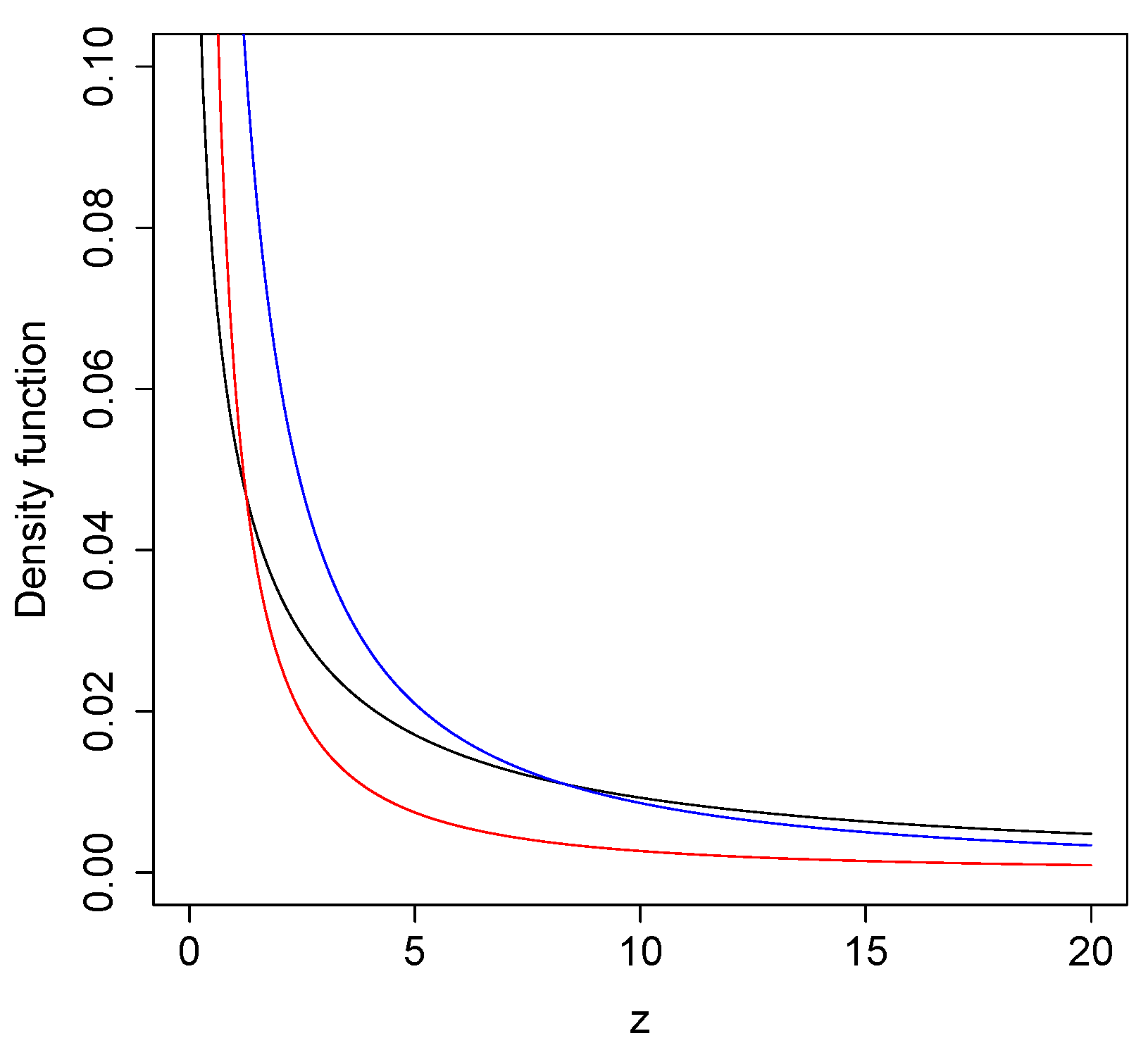
Figure 1 shows some plots of the SMG distribution considering different values of its parameters.

Figure 1.
Examples of SMG() (black), SMG() (blue), and SMG() (red) model.
Table 1 shows for different values of z in the SMG distribution, illustrating that the tails are heavier as the parameter decreases.

Table 1.
Tails comparison.
2.2. Properties
The following propositions show one way of representing the SMG distribution. The first proposition shows that the SMG distribution is the product of a scale mixture between the G and Beta.
Proposition 1.
Let and U∼; then, Z∼
Proof.
Calculating the integral directly, we have
the result of which is obtained with a change in variable . □
Proposition 2.
Let X∼ and Y∼ be independent random variables. Then, ∼
Proof.
Using the Jacobian method, we have
Then, marginalizing with respect to the variable V, we obtain the density function associated with Z:
By making the change in variables , the result is obtained. □
Two algorithms can be used to generate random numbers from the SMG model, as shown below. Algorithm 1 uses Proposition 1 and the composition method (see Tanner [20]); Algorithm 2 uses the representation given in Proposition 2.
| Algorithm 1 for simulating can proceed as follows |
|
Lemma 1.
Let . Then, we have the following:
- 1.
- 2.
| Algorithm 2 for simulating can proceed as follows |
|
Proof.
Both results are obtained directly using the pdf given in (3). □
Proposition 3.
Let Z∼. Then, the cdf of Z is given by
where , , , and is the regularized incomplete beta function.
Proof.
Applying the cdf definition directly, we have
By applying the integration by parts method and considering , the result is obtained. □
The survival function , which is the probability that an item will not fail before time t, is defined by . The survival function for an SMG random variable is given by
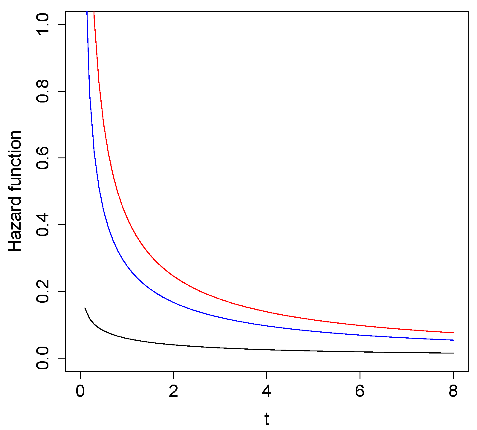
where . The hazards function , defined by , for an SMG random variable is given by
Figure 2 shows the shape of the hazards function for different values of , considering .
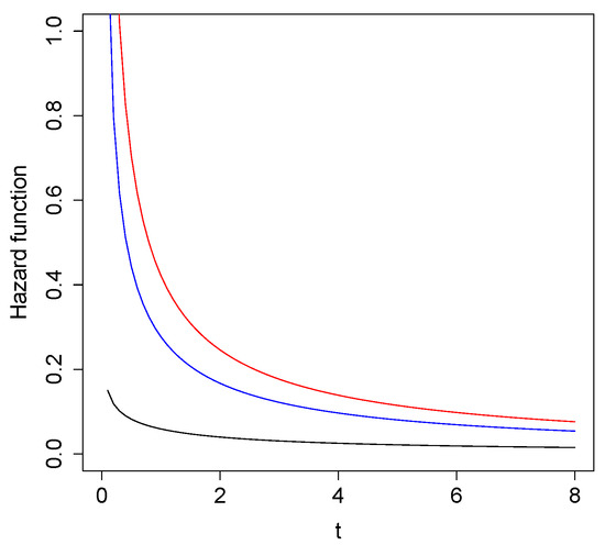
Figure 2.
Examples of for (black), (blue), and (red).
Proposition 4.
Let T∼. Then, the hazards function of T is decreasing for all .
Proof.
Using the Theorem, item , given in Glaser [21], we have
where is the pdf given in (3). Then, deriving the function with respect to t, we have
and the result is concluded. □
Figure 3 shows, by fixing , that the function is always negative. For other different values of and , the result is the same.
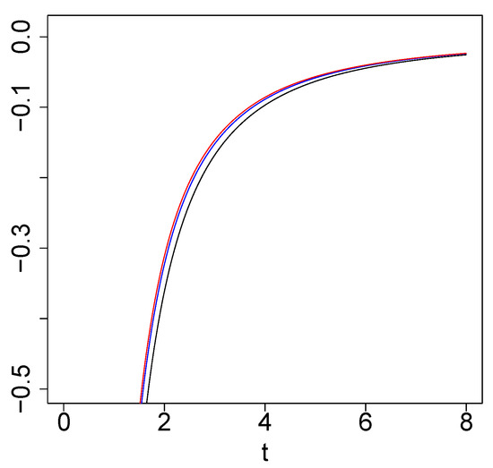
Figure 3.
Examples of for (black), (blue), and (red).
Proposition 5.
The rth moments of the random variable Z∼ do not exist for .
Proof.
Using integration by parts, with , we have
The expression on the left side is equal to zero if and does not exist if ; the integral on the right side was analyzed in Proposition 1 (e) of the work of Olmos et al. [18] and does not converge. Therefore, the complete integral diverges, and this means that no rth moments exist for the random variable Z∼. □
2.3. Tail of the Distribution
The Pareto model is a distribution with heavy right tail. Based on this characteristic, it is used in insurance to model the number of losses; hence, the size of the tail of the distribution is fundamental if the chosen model is to capture observations very distant from the start of the distribution support, i.e., extreme values. The concept of heavy tail is fundamental for this and other financial scenarios. The use of distributions with a heavy right tail is of vital importance in economics, finance, and natural disasters. Pareto, EP, and log normal distributions, among others, have been used to model losses in insurance, reinsurance, and catastrophic insurance. It is known that any distribution of probability, specified by its cdf on the real line, has a heavy right tail (see Rolski et al. [22]) if .
An important subject in the theory of extreme values is regular variation (see Bingham [23]). This concept is formalized in the following definition.
Definition 1.
A distribution function is called regular varying at infinity with index if
where the parameter is called the tail index.
The following proposition establishes that the survival function of the SMG distribution is a distribution with regular variation.
Proposition 6.
The survival function of the random variable is a survival function with regularly varying tails.
Proof.
Applying the above definition and using L’Hospital’s Rule, we have
and by calculating the latter limit, the result is obtained. □
3. Inference
In this section, we estimate the parameters of the SMG model using the ML method; a simulation study and asymptotic estimation of the ML estimators are discussed.
3.1. ML Estimation
For a random sample derived from the SMG() distribution, the log-likelihood function can be written as
Setting the first derivatives equal to zero with respect to each parameter, we have
where is the digamma function. From (6), we obtain
and the maximum likelihood estimator for () is obtained by numerically resolving the following equation:
The estimator is the solution to Equation (8), and replacing it in (7), we obtain . The solution for Equation (8) can be obtained by using numerical procedures such as the Newton–Raphson algorithm. Alternatively, these estimates can be found by directly maximizing the log-likelihood surface given by (5) and using the optim subroutine in the R software package [24].
3.2. Simulation Study
To evaluate the effectiveness of the proposed approach, we conducted a simulation study to assess the performance of the estimation procedure for the parameters and in the SMG model. The study involved simulating 1000 samples from the SMG model with three different sample sizes: n = 100, 200, and 300. Table 2 shows the median of the bias estimate for each parameter (Bias), its standard errors (SE), and the estimated root of the mean squared error (RMSE); the empirical coverage probabilities (CPs) at 95% for the asymptotic intervals based on ML estimators are given. From Table 2, we conclude that the ML estimates are quite stable. The bias is reasonable and reduced when the sample size is increased. The empirical CP also comes closer to the nominal 95% as n increases.
Table 2.
ML estimations for parameters and of the SMG distribution.
3.3. Fisher’s Information Matrix
Let us now consider . For a single observation z of Z, the log-likelihood function for is given by
The corresponding first and second partial derivatives of the log-likelihood function are derived in Appendix A. It can be shown that the Fisher’s information matrix, denoted by , for the G distribution is provided by
where is the trigamma function and .
Hence, for large samples, the ML estimator, , of is asymptotically normal bivariate, that is, the following is true;
the asymptotic variance of the ML estimator is, therefore, the inverse of Fisher’s information matrix Since the parameters are unknown, the observed information matrix is usually considered, where the unknown parameters are estimated by ML.
4. Application with Real Data
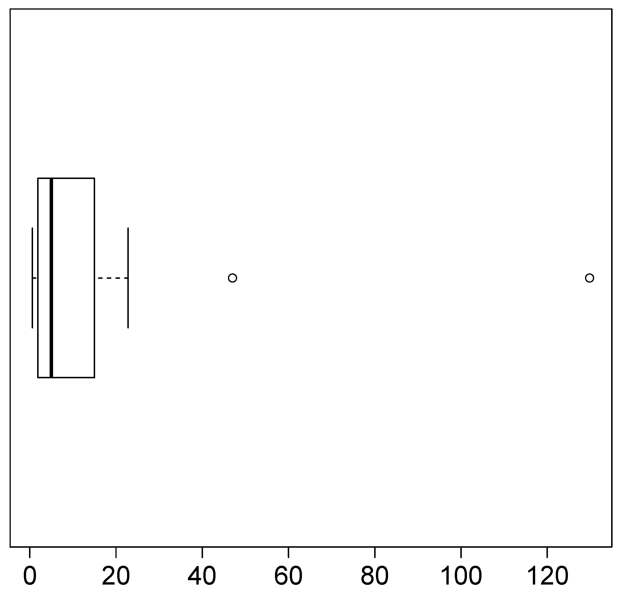
In this section, we analyze an application to a real dataset, comparing the Pareto and LG2 distributions with the fit of the SMG distribution. To compare the models, we use the Akaike information criterion, AIC (see Akaike [25]), and the Bayesian information criterion, BIC (see Schwarz [26]). The dataset represents accident indices (annual data in billions of USD) for earthquake insurance in California from 1971 to 1993 for values greater than zero. The data are given in Embrechts et al. [27]. The descriptive statistics of these data are shown in Table 3, where CS is the coefficient of asymmetry of the sample, and CK is the coefficient of kurtosis of the sample. The CK is quite high, and this shows the presence of atypical observations. The boxplot in Figure 4 shows the existence of two very extreme data. These atypical data make the right tail heavier.
Table 3.
Descriptive statistics for loss ratios data.

Figure 4.
Boxplot for of loss ratios data.
Table 4 shows the ML estimates together with standard errors (in brackets) for the parameters of the SMG, Pareto, and LG2 models, as well as the values of the AIC and BIC criteria for each model. For the Pareto and LG2 models, the value was used.
Table 4.
Loss ratios data: model, ML estimates, and AIC and BIC values.
We observe that the smallest values of the AIC and BIC criteria correspond to the SMG model, meaning that the SMG model fits the data better than the Pareto and LG2 models. The SEs of the ML of the SMG model were calculated using the method described in Section 3.3.
Table 5 shows three goodness-of-fit tests for all the distributions considered; this shows that the classic Pareto distribution is rejected for this dataset.
Table 5.
Test statistics (p-values) of goodness-of-fit tests of the considered models.
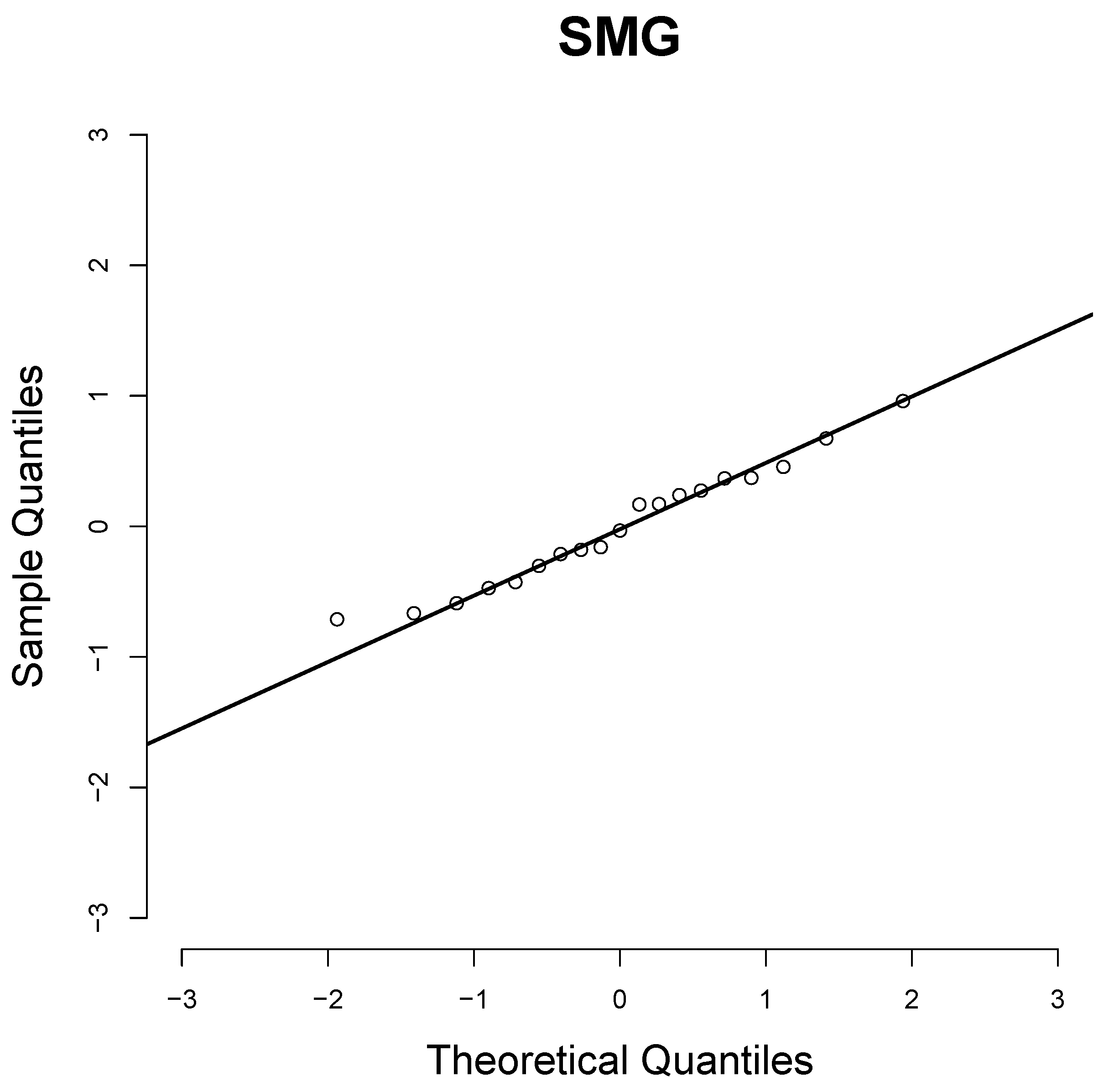
We observe that the goodness-of-fit tests indicate that the SMG and LG2 distributions are appropriate for fitting these data; the selection criteria of the AIC and BIC models indicate that the SMG distribution provides a better fit than the other two. For this reason, the SMG distribution may be considered as an alternative to the classic Pareto distribution. Figure 5 shows the Q–Q plot of the quantile residuals (QRs) of the SMG distribution (see Dunn and Smyth [28]).
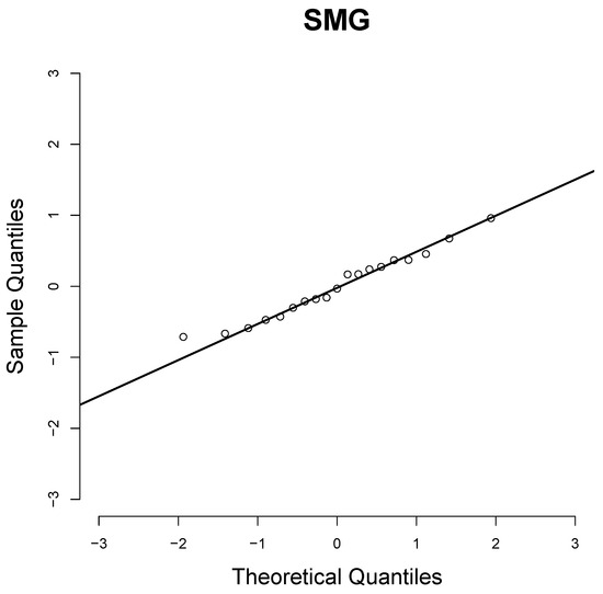
Figure 5.
Q–Q plots of the QRs for SMG distribution.
5. Conclusions
This paper presents a study of the SMG distribution; we study some of its properties, estimate the parameters using the ML method, and analyze an application to real data. The SMG distribution is the product of a scale mixture of the G and Beta distributions. This distribution has two parameters, making it interesting as a competitor with several two-parameter models used, for example, in actuarial statistics. The SMG model appears to be a viable alternative for fitting data with atypical observations. Some other characteristics of the SMG model are as follows:
- The right tail of the SMG model is heavier for small values of parameter .
- There are representations of the SMG model, given in Propositions 1 and 2.
- The SMG distribution has a heavy right tail, see Proposition 6.
- The pdf, cdf, and hazard function are explicit and are represented by known functions.
- The analysis of the application shows that the SMG distribution is a good candidate for modeling loss ratios data, performing better than two well-known distributions, the Pareto and LG2 distributions.
Author Contributions
Conceptualization, N.M.O. and E.G.-D.; methodology, N.M.O. and E.G.-D.; software, N.M.O. and E.G.-D.; validation, N.M.O., E.G.-D. and O.V.; formal analysis, N.M.O. and O.V.; investigation, E.G.-D. and N.M.O.; writing—original draft preparation, N.M.O. and E.G.-D.; writing—review and editing, O.V. and E.G.-D.; funding acquisition, O.V. All authors have read and agreed to the published version of the manuscript.
Funding
The research work by N.M. Olmos was supported by Semillero UA-2024.
Institutional Review Board Statement
Not applicable.
Informed Consent Statement
Not applicable.
Data Availability Statement
The data set is available in the text.
Conflicts of Interest
The authors declare no conflicts of interest.
Appendix A
The first derivatives of are given by
The second derivatives of are
where and are the digamma and trigamma functions, respectively.
References
- Pareto, V. Cours d’Éconimie Politique; Librairie Droz: Laussanne, Switzerland, 1897. [Google Scholar]
- Beirlant, J.; Teugels, J.L.; Vynckier, P. Practical Analysis of Extreme Values; Leuven University Press: Leuven, Belgium, 1996. [Google Scholar]
- Beirlant, J.; Joossens, E.; Segers, J. Generalized Pareto fit to the society of actuaries’ large claims database. N. Am. Actuar. J. 2004, 8, 108–111. [Google Scholar] [CrossRef]
- Resnick, S.I. Discussion of the Danish data on large fire insurance losses. ASTIN Bull. 1997, 27, 139–151. [Google Scholar] [CrossRef]
- Johnson, N.L.; Kotz, S.; Balakrishnan, N. Continuous Univariate Distributions, 2nd ed.; Wiley Series in Probability and Statistics; Wiley: New York, NY, USA, 1995. [Google Scholar]
- Pickands, J. Statistical inference using extreme order statistics. Ann. Stat. 1975, 3, 119–131. [Google Scholar]
- Choulakian, V.; Stephens, M.A. Goodness-of-fit for the generalized Pareto distribution. Technometrics 2001, 43, 478–484. [Google Scholar] [CrossRef]
- Davison, A.C.; Smith, R.L. Models for Exceedances Over High Thresholds (with comments). J. R. Stat. Soc. Ser. B 1990, 52, 393–442. [Google Scholar] [CrossRef]
- Aban, I.B.; Meerschaert, M.M.; Panorska, A.K. Parameter estimation for the truncated Pareto distribution. J. Am. Statist. Assoc. 2006, 101, 270–277. [Google Scholar] [CrossRef]
- Gupta, R.C.; Gupta, R.D.; Gupta, P.L. Modeling failure time data by Lehman alternatives. Commun. Stat. Theory Methods 1998, 27, 887–904. [Google Scholar] [CrossRef]
- Stoppa, G. Proprieta campionarie di un nuovo modello Pareto generalizzato. In Proceedings of the Atti XXXV Riunione Scientifica della Societa Italiana di Statistica, Padova, Italy, 18–21 April 1990; Cedam: Padova, Italy, 1990; pp. 137–144. [Google Scholar]
- Kleiber, C.; Kotz, S. Statistical Size Distributions in Economics and Actuarial Sciences; John Wiley & Sons: Hoboken, NJ, USA, 2003. [Google Scholar]
- Akinsete, A.; Famoye, F.; Lee, C. The Beta-Pareto distribution. Statistics 2008, 42, 547–563. [Google Scholar] [CrossRef]
- Boumaraf, B.; Seddik-Ameur, N.; Barbu, V.S. Estimation of Beta-Pareto Distribution Based on Several Optimization Methods. Mathematics 2020, 8, 1055. [Google Scholar] [CrossRef]
- Arnold, B.C. Pareto Distributions. In Monographs on Statistics & Applied Probability, 2nd ed.; Chapman & Hall: Boca Raton, FL, USA, 2015. [Google Scholar]
- Gómez-Déniz, E.; Calderín-Ojeda, E. A suitable alternative to the Pareto distribution. Hacet. J. Math. Stat. 2014, 43, 843–860. [Google Scholar]
- Gleser, L.J. The Gamma Distribution as a Mixture of Exponential Distributions. Am. Stat. 1989, 43, 115–117. [Google Scholar] [CrossRef]
- Olmos, N.M.; Gómez-Déniz, E.; Venegas, O. The Heavy-Tailed Gleser Model: Properties, Estimation, and Applications. Mathematics 2022, 10, 4577. [Google Scholar] [CrossRef]
- Andrews, D.F.; Mallows, C.L. Scale mixtures of normal distributions. J. R. Stat Soc. Ser. B 1974, 36, 99–102. [Google Scholar] [CrossRef]
- Tanner, M.A. Tools for statistical inference. In Methods for the Exploration of Posterior Distributions and Likelihood Functions, 3rd ed.; Springer: New York, NY, USA, 1996. [Google Scholar]
- Glaser, R.E. Bathtub and Related Failure Rate Characterizations. J. Am. Stat. Assoc. 1980, 75, 667–672. [Google Scholar] [CrossRef]
- Rolski, T.; Schmidli, H.; Schmidt, V.; Teugel, J. Stochastic Processes for Insurance and Finance; John Wiley & Sons: Hoboken, NJ, USA, 1999. [Google Scholar]
- Bingham, N. Regular Variation; Cambridge University Press: Cambridge, UK, 1987. [Google Scholar]
- R Core Team. R: A Language and Environment for Statistical Computing; R Foundation for Statistical Computing: Vienna, Austria, 2021; Available online: https://www.R-project.org/ (accessed on 15 January 2024).
- Akaike, H. A new look at the statistical model identification. IEEE Trans. Automat. Cont. 1974, 19, 716–723. [Google Scholar] [CrossRef]
- Schwarz, G. Estimating the dimension of a model. Ann. Statist. 1978, 6, 461–464. [Google Scholar] [CrossRef]
- Embrechts, P.; Sidney, I.R.; Gennady, S. Extreme value theory as a risk management tool. N. Am. Actuar. J. 1999, 3, 30–41. [Google Scholar] [CrossRef]
- Dunn, P.K.; Smyth, G.K. Randomized Quantile Residuals. J. Comput. Graph. Stat. 1996, 5, 236–244. [Google Scholar] [CrossRef]

Disclaimer/Publisher’s Note: The statements, opinions and data contained in all publications are solely those of the individual author(s) and contributor(s) and not of MDPI and/or the editor(s). MDPI and/or the editor(s) disclaim responsibility for any injury to people or property resulting from any ideas, methods, instructions or products referred to in the content. |
© 2024 by the authors. Licensee MDPI, Basel, Switzerland. This article is an open access article distributed under the terms and conditions of the Creative Commons Attribution (CC BY) license (https://creativecommons.org/licenses/by/4.0/).