Abstract
The Dynamic Interval (DI) graph models the updating uncertainty of the arc cost in the graph, which shows great application prospects in unstable-road transportation planning and management. This paper studies the Real-time Shortest Path (RTSP) problems in the DI graph. First, the RTSP problem is defined in mathematical equations. Second, three models for RTSP are proposed, which are the Dynamic Robust Shortest Path (DRSP) model, the Dynamic Greedy Robust Shortest Path (DGRSP) model and the Dynamic Mean Shortest Path (DMSP) model. Then, three solution methods are designed. Finally, a numerical study is conducted to compare the efficiency of the models and corresponding solution methods. It shows that the DGRSP model and DMSP model generally present better results than the others. In the real road network test, they have the minimum average-regret-ratio of DGSP 7.8% and DMSP 7.1%; while in the generated network test, they both have a minimum average-regret-ratio of 0.5%.
Keywords:
dynamic interval graph; real-time shortest path; nested Dijkstra algorithm; dynamic vehicle routing MSC:
90-10
1. Introduction
With the fast development of Global Positioning System (GPS) technologies and the wide use of mobile phones, innovative services have emerged, such as electronic maps, ride-sharing and ride-hailing. Among these services, static and dynamic Vehicle Routing (VR) functions are frequently used, especially in unstable-road transportation. It mainly helps the traveler find the Real-time Shortest Path (RTSP) from the starting position (node) to the destination position (node).
There are six kinds of Shortest Paths for VR functions corresponding to six kinds of graphs (see Table 1 and Figure 1).

Table 1.
Six kinds of shortest path problems in six graphs.
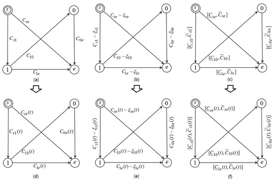
Figure 1.
Six kinds of graphs. (a) SD graph; (b) SS graph; (c) SI graph; (d) DD graph; (e) DS graph; (f) DI graph.
The Static and Deterministic (SD) graph and Shortest Path (SP) problem (Figure 1a). In the SD graph, the cost of each arc is directly known. Dijkstra [1] first studies the SP problem in the SD graph, and designs a famous dynamic programming algorithm, named the Dijkstra algorithm. Then, the Floyd–Warshall algorithm and Bellman–Ford algorithm are proposed for the SP problem by Floyd [2], Bellman [3] and Ford and Fulkerson [4]. Himmich et al. [5] study an extension of the SP problem. In addition to the deterministic arc cost, the resource constraints are considered in an R-dimensional resource consumption vector. A multi-phase dynamic programming algorithm is designed to solve the model. Bahel et al. [6] study an application of the SP in the area of agents shipping their respective demands, that is, more than one traveler (visitor) should find their SPs in the model.
The Dynamic and Deterministic (DD) graph and Dynamic Shortest Path (DSP) problem (Figure 1d). In the DD graph, the cost of each arc changes over time (or stage) t. Previous work on algorithms for DSP problems in DD graph includes Murchland [7], Dionne [8], and Goto and Sangiovanni–Vincentelli [9]. Then, Ramalingam and Reps [10] develop a widely-used algorithm, named RR. It presents good performance in most situations. By observing that the RR algorithm updates, in the data structure aspect, the shortest path graph instead of the shortest path tree, Demetrescu, et al. [11] propose a specialization of the RR algorithm for updating a shortest path tree. Then, Buriol, et al. [12] introduce a new generic technique to reduce the heap (priority queue) size.
The Static and Stochastic (SS) graph and Stochastic Shortest Path (SSP) problem (Figure 1b). The cost of each arc in the graph is modeled by an independent random variable. Martin [13] studies the shortest path in stochastic networks, which is also directed and acyclic. Then, Frank [14] and Hassin and Zemel [15] study the stochastic graph where all the arcs’ cost is known before entering into the network and the goal is to find the shortest path in this implementation. Mirchandani and Soroush [16,17] assume that the actual cost of all arcs is unknown before the path is selected, and the goal is to choose a path that minimizes the expected total cost. Beigy and Meybodi [18] study the SSP with the positive-valued random variable arc cost sampled from a distribution, and an iterative stochastic algorithm using a distributed learning automata to find the SSP by taking a sufficient number of samples. Ketkov et al. [19] study the SSP with the arc cost subject to distributional uncertainty, and the decision-maker minimizes the worst-case expected loss over an ambiguity set (or a family) of candidate distributions. It is the combination of stochastic uncertainty and interval uncertainty. Lee et al. [20] study the SSP to maximize the probability of arriving at the destination within a given time budget with the arc cost (travel time) following an independent normal distribution and develop pseudo-polynomial time exact algorithms. Song and Cheng [21] concentrate on the SSP problem with the mean and standard deviation of arc cost (travel time) directly known. They transform the problem into a mixed-integer conic quadratic program and design a generalized Bender’s decomposition solution approach.
The Dynamic and Stochastic (DS) graph and Dynamic Stochastic Shortest Path (DSSP) problem (Figure 1e). The cost of each arc in the graph is modeled by a random variable depending on time. Hall [22] studies the stochastic network with travel times that are both random and time-dependent. The goal is to find the least expected travel time path. It is concluded that an adaptive decision rule is better than a simple path. Bertsimas and Van Ryzin [23,24] study the stochastic and dynamic vehicle routing problem, where vehicles traveling at constant velocities must serve stochastic demands. Psaraftis and Tsitsiklis [25] examine the SP problems, where the arc costs are the known functions of certain environmental variables following independent Markov dynamic processes. For more relevant research see Azaron and Kianfar [26], Pattanamekar et al. [27], and Ojeda Rios et al. [28].
The Static and Interval (SI) graph Robust Shortest Path (RSP) problem (Figure 1c). The cost of each arc in the graph is uncertain and modeled by an interval value. Dias and Climaco [29] first study the Robust Shortest Path (RSP) problem in an interval graph. Averbakh and Lebedev [30] and Zielinski [31] simultaneously prove the NP-hardness of the RSP problem. Karasan et al. [32] introduce a mixed integer programming (MIP) formulation for the RSP problem. Then, Montemanni et al. [33] present a branch and bound algorithm for RSP, while Montemanni and Gambardella [34] give an exact algorithm based on Benders decomposition. The approximate algorithm for RSP is designed by Kasperski and Zielinski [35]. Catanzaro et al. [36] reduce the search domain by giving sufficient conditions for nodes and arcs which are always (or never) in an optimal solution. Chassein et al. [37] consider RSP problems to find a path that optimizes the worst-case performance over an uncertainty set for arc costs where one of the uncertainty measures is the interval uncertainty. The data-driven robust optimization is conducted based on real-world traffic measurements from Chicago City. Davoodi and Ghaffari [38] model the uncertain networks with interval arc. To find the SP, they propose a practical approach with two phases, that is, a preprocessing phase and a query phase. Zhang [39] studies the unique shortest path routing problem, which aims to find an optimal weight set subject to four sets of constraints. Interval arc cost appears as a set constraint of link capacity.
The Dynamic and Interval (DI) graph Dynamic Robust Shortest Path (DRSP) problem (Figure 1f). The cost of each arc in the graph is uncertain and modeled by an interval value depending on time. Compared to the SI graph, the DI graph makes full use of the updated information and shows great application prospects in the transportation application. Xu and Zhou [40] study the Dynamic Robust Shortest Path (DRSP) problem in the DI graph. The Nested Dijkstra (ND) algorithm is given as a heuristic algorithm.
This paper concentrates on the DI graph. First, a general formula of the RTSP problem in the DI graph is given. Then, instead of the DRSP model, two models are proposed, which are the Dynamic Greedy Robust Shortest Path (DGRSP) model and the Dynamic Mean Shortest Path (DMSP) model. The DRSP model considers the uncertainty of all arcs equally; the DGRSP model considers more about the uncertainty of the nearby arcs; the DMSP model uses the interval mean value to approximately replace the uncertainty. Then, three solution methods are designed for the corresponding three models, which are the CPLEX optimizer, ND algorithm and Dijkstra algorithm. Finally, a numerical study is conducted in both real road networks and generated networks to validate the efficiency of the models and algorithms. It shows that the DGRSP model and ND algorithm generally return the best solution.
This paper is organized as follows: The SP problem in the DI graph is formally described in Section 2. The DRSP model, DGRSP model and MSP model, as well as their corresponding algorithms and solution methods, are the main body of this paper. They are described in Section 3, Section 4 and Section 5, respectively. In Section 6, the numerical study is conducted, which validates the efficiency of the models and algorithms. The main conclusions are summarized in Section 7. The abbreviations used in this paper are in Table 2.
Table 2.
Most used abbreviations in this paper.
2. Problem Definition
The DI graph aims to model the real-time variation of the graph. The RTSP problem in the DI graph is proposed for two reasons. First, in unstable areas such as earthquake rescue areas and war rescue zones, it tries to reduce the timely uncertainty and helps more people escape from difficulties; second, in daily transportation, it timely reduces the uncertainty and improves the scheduling efficiency. The real-time tracking system including GPS makes this operation possible. The RTSP model returns the real-time solution path with the next visiting node which forms the final routing path with minimized cost for the traveler. Compared to the traditional SP, it dynamically changes routes with time and controls the uncertainty by interval cost and minimized regret.
Suppose is a directed graph with nodes set V and arcs set A, , . Node s is the starting (origin) node, and e is the end (destination) node, . Suppose p is a path from s to e, and P is a path set containing all paths from s to e. At least one path p, from s to e, exists in the graph G. We have and . When the visitor in stage t stays at a node in the graph, there are k frozen nodes determined to visit for the next k stages, which are . Generally, the number of frozen nodes is often 1 or 2 in the transportation model, that is, . Too many frozen nodes may reduce the usage of the updated information. We optimize the path from to e.
At the beginning of initialization, SP finds an optimized path from to e to initiate the frozen nodes set (see in Figure 2a). In the first stage, the visitor stays at node s, and . The frozen nodes are . It visits node in the path directly connected to , finds an optimized path from to e, and adds node to the frozen node set. At the 2nd stage, the visitor stays at node . The frozen nodes become . It visits node , finds an optimized path from to e, and adds node to the frozen node set. So again, at the tth stage, the frozen nodes are . The visitor visits node , finds an optimized path from to e, and adds node to the frozen node set, . Finally, suppose at the th stage, the visitor reaches the destination node e, and finishes the travel with . So the whole path is .
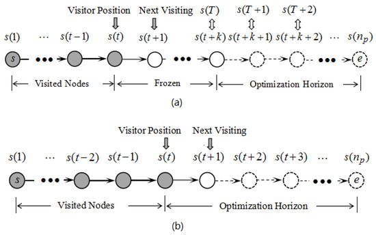
Figure 2.
Optimization horizon for visitors in stage t. (a) With frozen nodes; (b) without frozen nodes.
The possible cost of arc in stage t is in the interval , that is, (see in Figure 1f). is known in stage t, and thus in the final stage the problem is a DSP problem (offline problem), and the optimal path can be calculated by dynamic programming. However, before stage , it is an online problem, only God knows the optimal path. In the real-world application scenario, the road may face extreme variations such as sudden closures. It can be modeled by setting with a large number if the closures happen in stage t.
The objective of online RTSP is to find the shortest path, with minimized cost, from s to e. Suppose is a path p from s to e in path set P. Then, the objective is
which compares all possible paths in P to achieve the optimal path. The variable of arc cost is essential since it affects the final total cost. Suppose the final offline optimal path for RTSP from s to e is , where , , and . Then, the length of the optimal path is
By comparing Equation (1) and (2), the difference between and is defined as the regret . Minimizing is equivalent to minimizing , since is a constant value.
Since it is scarcely possible to obtain the optimal solution before stage n, we can construct a dynamic model (see Figure 2a). That is, find an optimal path in each stage , add the corresponding node in the frozen nodes set, and finally construct an acceptable path. The following are three dynamic models and the corresponding solution methods for the RTSP problem in stage t.
3. DRSP Model in DI Graph
3.1. Problem Description
The DRSP model is an extension of RSP to the dynamic version to make the full usage of the updated information. Figure 3 gives an example to show its advantage. DRSP in Figure 3 controls the realization of the maximum regret , which is also shown in Table 3.
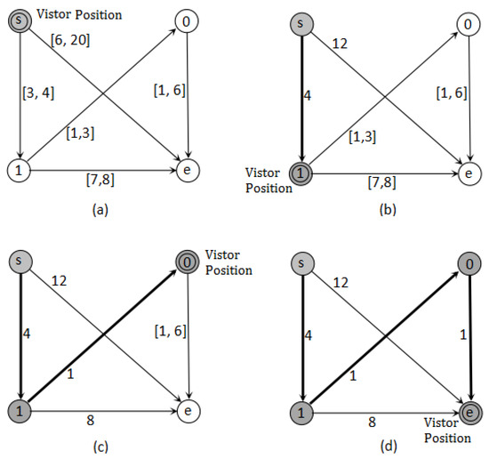
Figure 3.
An example to show the advantage of the DRSP. (a) the visitor starts at node s; (b) the visitor reaches node 1; (c) the visitor reaches node 0; (d) the visitor finally reaches node e.
Table 3.
Maximum regret relates to the visitor’s location in DRSP.
When the visitor starts at node s (in Figure 3a), path {s,1,e} is the optimal path with the minimized maximum regret of 6 which is achieved by Definition 1–4. If we use this result without any change, it is the static RSP model with the final regret of 6. However, the updated information of arc and may be used when the visitor stays in node 1 (in Figure 3b), which results in the new optimal path of {s,1,0,e} with minimized maximum regret 2. When the visitor reaches node 0 (in Figure 3c) and the node e (in Figure 3d), path {s,1,0,e} is still optimal with the regret 0. That is to say, the static RSP model only gives the fixed path {s,1,e} with the final realization of regret 6. However, the DRSP uses the updated information to change the path in node 1 from {s,1,e} to {s,1,0,e} resulting in the final realization of regret reduced to 0. Figure 3 and Table 3 make a mini-correction of that in Xu and Zhou [40].
The DRSP model finds in each stage t the robust path which minimizes the robust cost (maximum deviation from the optimal shortest path) from node to e, . Then, it adds the nearby node in the optimal path to the frozen nodes set. It is formally described by the following four definitions with .
Definition 1.
A scenario r is a realization of all arc costs, that is, in scenario r, the cost is fixed, .
Definition 2.
The robust deviation (RD), in a scenario r for path p from to e, is the difference between p path cost in r and the SP cost in r from to e.
Definition 3.
A robust cost (RC) for path p from to e is the maximum RD for p among all possible scenarios, that is, .
Definition 4.
The DRSP aims to find the path p among all paths from to e at stage t with the minimized RC.
Theorem 1 is known in the literature for simplifying the RC calculation, where only the scenario induced by path p should be considered in stage t. Take Figure 3a for example, the scenario induced by path is depicted in Figure 4. The RC of p is .
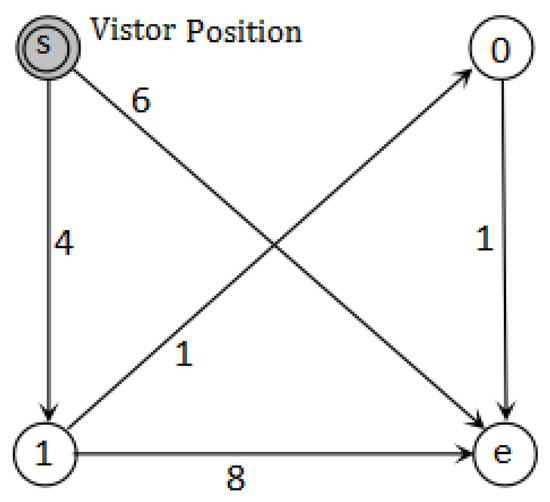
Figure 4.
The scenario induced by path .
Theorem 1
(Karasan et al. [26]). The RD for path p is maximized in the scenario induced by p where the costs of all arcs in p are at upper bounds and the costs of all other arcs are at lower bounds.
3.2. Mixed Integer Programming (MIP) Formulations
The MIP formulations for the DRSP problem for path p in stage t () are given as follows based on Theorem 1. Let , then the optimization horizon in stage t is .
The objective (3) searches for a path p with minimized RC at stage t, where is a binary vector representing a path by constraint (5). If , arc is in the DRSP; 0 otherwise. Variable denotes the shortest total cost from node to j in the scenario induced by . Then, is the cost of the shortest path from to e in this scenario.
In constraint (4), for a given vector , the cost of arc is . It follows Theorem 1 to set the cost of arc at its upper bound on path p with , and all the costs of other arcs at lower bounds with .
Constraints (6)–(8) initialize the problem and define the domains of all the variables.
The MIP model (3)–(8) is solved by CPLEX Optimization Studio 12.5 in the numerical study in Section 6.
4. DGRSP Model in DI Graph
In the dynamic model in Figure 2a, the recently frozen node is more important than the other far nodes in the optimal path of DRSP in stage t. Because the road information is timely updated, which results in the other far nodes hardly on the optimal path in the following stage. From this point, the Dynamic Greedy Robust Shortest Path (DGRSP) model is proposed, which is a modification and improvement of the DRSP model. By paying more attention to the nearby nodes, DGRSP first constructs the optimal path from to the nearby nodes and then expands the path to the other nodes. We call it the greedy strategy.
4.1. Problem Description
For the traveler in stage t, the optimization horizon is still , where , . The objective of DGRSP for any node in the optimal path is calculated by
Note that the DGRSP in stage t is also a DRSP if all the subpath , of the DRSP , is also a DRSP from to f. Theorem 2 proves the relationship between DGRSP and DRSP.
Theorem 2.
The DGRSP is also a DRSP in stage t in the DI graph , if is still a DRSP for any node in DRSP .
Proof.
First, path is obviously the DRSP and DGRSP since it has only one node.
Second, suppose the path is the DRSP and DGRSP, then the path achieved by Equation (9) is a DGRSP. Obviously, it is also a DRSP. Otherwise, there are two conditions.
(1) Suppose there exists another node to form a DRSP path . Then, the path should have a smaller RC than the path . Contradictions arise since Equation (9) is violated.
(2) Suppose there exists another node to form a DRSP path . Then, the path , , ⋯, are all DRSPs with minimized RC and should be identified by Equation (9). The RC of should not be smaller than that of . Contradictions arise.
In conclusion, the DGRSP is also a DRSP in stage t, if is still a DRSP for any node in DRSP . □
4.2. Nested Dijkstra Algorithm for DGRSP
The Nested Dijkstra (ND) is a dynamic programming algorithm developed by Xu and Zhou [40]. It can effectively solve the DGRSP here.
ND is constructed with a Dijkstra algorithm nested by another Dijkstra algorithm, where the Dijkstra algorithm refers to Dijkstra [1]. The inner Dijkstra algorithm computes the robust cost (RC) of a path, while the external Dijkstra algorithm determines the final solution for the DGRSP (see Figure 5).
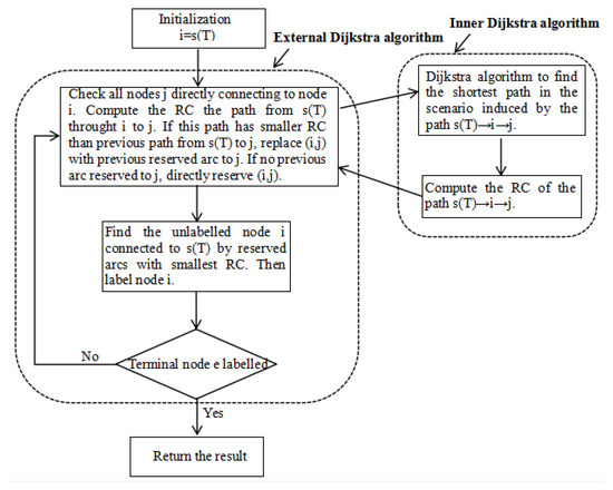
Figure 5.
Structure of ND algorithm.
Theorem 3, proven by Xu and Zhou [40], shows that the inner Dijkstra algorithm can calculate out the RC. Theorem 4 proves that ND returns the optimal solution of the DGRSP. Theorem 5 is the time complexity of the ND algorithm.
Theorem 3
(Xu and Zhou [40]). The robust cost of all paths can be determined by the inner Dijkstra algorithm with a time complexity of .
Theorem 4.
The ND algorithm returns the optimal solution of DGRSP.
Proof.
First, for any nodes directly connected to , the ND algorithm returns the solution with the minimized RC.
Second, suppose, for any node , the ND algorithm returns the solution with the minimized RC. Then, for node v, ND returns the solution with the minimized RC under the consideration of the minimized RC solution path from to .
Finally, the optimal solution of DGRSP from to e is returned by the ND algorithm. □
Theorem 5.
The ND algorithm returns the optimal solution of DGRSP with the time complexity of .
Proof.
First, the inner Dijkstra algorithm calculates the RC for a path costs time of (see in Theorem 2).
Second, the external Dijkstra algorithm needs to consider all the arcs in the graph. The arc number is at most , and the time-complexity is also .
Thus, the total time complexity of the ND algorithm is . □
The pseudo-code for the ND algorithm is shown in detail as follows (Algorithm 1): it is applied in the numerical study in Section 6.
| Algorithm 1: ND algorithm |
; %Initialization while node e unlabeled do %Terminal check :=a set of unlabeled nodes directly connected to i; for iteration do %Update the RC of nodes in Compute by inner Dijkstra from through i to j; if no previous reserved arc from directly or indirectly to j; then reserve arc ; else then compare with the RC of previous path to j; reserve the smaller one instead of the previous one; end if end :=a set of unlabeled nodes; ; for iteration do %Find unlabeled nodes with min RC if then ; end if end for Label i and reserve the corresponding arc directly or indirectly to ; end return the RC of all nodes and all the reserved arcs; %Final result |
5. DMSP Model in DI Graph
The Dynamic Mean Shortest Path (DMSP) model in stage t has the optimization horizon of , where , . Suppose has the equal possibility in the interval of , then we let , that is, the uncertain arc has the mean cost of in stage t. The MIP formulations are shown in (10)–(12).
The objective (10) searches for a path p with minimized mean cost at stage t, where is a binary vector representing a path by constraint (11). If , arc is on path p; 0 otherwise.
Constraint (12) initializes the problem. implies that ; otherwise, constraint (11) is violated.
Theorem 6.
The Dijkstra algorithm (or inner Dijkstra algorithm in ND algorithm) can be used to return the optimal solution of the DMSP model in stage t with the time-complexity of .
Proof.
In stage t, the DMSP problem is equivalent to an SP problem in the SD graph. The inner Dijkstra algorithm finds the SP in a scenario and can be used to solve the DMSP problem.
The inner Dijkstra algorithm needs to consider all the arcs in the graph. The arc number is at most , and the time complexity is then . □
The Dijkstra algorithm is used to solve the DMSP model in the numerical study in Section 6.
6. Numerical Study
The following presents proof-of-concept implementations of three models, as well as the corresponding solution methods, in the DI graph. Suppose . Since more traffic information is achieved as time passes, we assume . That is to say, we first assume a much bigger uncertainty, and then shorten the uncertainty with time for the schedule. In the real-world application scenario, it is necessary to carefully shorten the uncertainty with time to avoid the violation of this assumption.
There are four main metrics, which are cost, regret, regret ratio and CPU time to evaluate the effectiveness of the models and solution methods (see also in Table 4 and Table 5). Cost and regret measure the absolute cost and regret of the final path. The regret ratio measures the relative regret compared to the optimal offline path cost. CPU time measures the time cost of the algorithm to return the result. The implementations are carried out by Matlab 7.11.0 and CPLEX Optimization Studio 12.5 in a personal computer with Intel(R) Core(TM) i3-2310M CPU @ 2.10 GHz 2.10 GHz, RAM 4.00 GB and Win 7 OS.
Table 4.
Final solutions for five methods (in real roads).
Table 5.
Final solutions for five methods (in the generated network).
6.1. Real Roads Test
The real road data are selected from the examination questions in the National Postgraduate Mathematic Contest in Modeling in 2009 D in China. Figure 6 shows the real road network with 307 nodes (crossroads) and 458 arcs (roads). All of them are marked in Cartesian coordinates with the units in meters. A car runs from node s (14418, 8046) to node e (216, 414). The arc cost is restricted in the interval number of . is the distance between i and j, since the main arc cost, such as travel time cost and fuel cost, is related to the distance . is a random variable with uniform distribution , which models the uncertainty hitting leading the width change of the interval, and , . We suppose that the exact cost , ) of arc is known if the traveler is located in node in stage t because the road will be crossed immediately with the uncertainty being negligible (similar to Figure 3). The frozen nodes are ignored to strengthen the influence of the updated information (see Figure 2b).
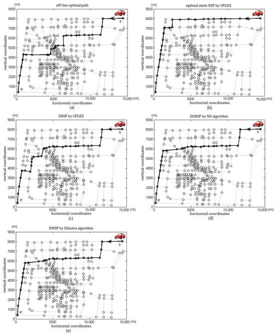
Figure 6.
A group of solutions in real road tests. (a) an off-line optimal path; (b) an optimal path for static RSP by CPLEX; (c) a path for DRSP by CPLEX; (d) a path for DGRSP by ND algorithm; (e) a path for DMSP by Dijkstra algorithm.
Table 4 presents a comparison of five methods. The “optimal” denotes the offline optimal path, which is calculated by the Dijkstra algorithm in stage n when all the final arc costs are fixed. The “Static RSP” is calculated out in the DRSP model by CPLEX in stage 1 from s to e. The “DRSP” is calculated out in the DRSP model by CPLEX in each stage with updating road information. The “DGRSP” is achieved in the DGRSP model by the ND algorithm by updating road information. The “DMSP” is achieved in the DMSP model by the Dijkstra algorithm by updating road information.
It is easy to know that the DGRSP model and DMSP model give the best two solutions compared to the other methods. They generally have the least average-regret-ratio of DGSP 7.8% and DMSP 7.1%, where . And CPLEX for Static RSP gives the worst solution with the maximum regret ratio because this model does not consider the updated information of the road cost. The computation time of four methods is all below 4 s, which is acceptable for decision.
Figure 6 illustrates a group of final solution paths by five methods in Table 4, while Figure 7 is the comparison of the regret ratio by four methods. The fluctuation happens since the arc cost is randomly generated. Generally, the DGRSP model and DMSP model give the best solutions. Although DRSP makes use of the updated information, it is generally not better than DGRSP and DMSP in most test cases. Besides, we can see that all methods present their advantages in some cases, in which they are better than the other methods. So, an integration of the four methods in the application should also be a valuable consideration.
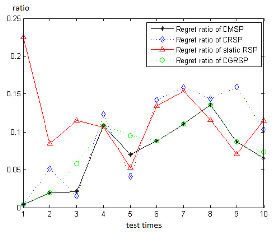
Figure 7.
Regret ratio of four methods (in real road network).
6.2. Generated Network Test
The following is the test of the generated network with n nodes. For long-distance transportation, the chosen route is often roughly in one direction. This network models the chosen nodes in the long and narrow range and roughly in one direction. The coordinate of the ith node is , where is a uniformly distributed random variable and models the uncertainty in this generation. We have , , and . Here, each node connects at most four neighbor nodes since the reality road network has nodes connecting rarely more than four neighbor nodes. For node , the cost of arc is in the interval of with
where is a uniform distributed random variable modeling the width of the interval, that is, , and , . Figure 8 shows an example of this network. The traveler (visitor) starts at the first node, and ends at the th node. In the DI graph, the traveler is supposed to know the exact cost , ) of the arc if it is located in node s (similar to the real road in Section 6.1).
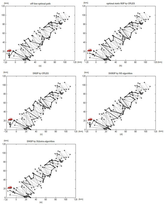
Figure 8.
A group of solutions by five methods with 100 nodes. (a) an off-line optimal path; (b) an optimal path for static RSP by CPLEX; (c) a path for DRSP by CPLEX; (d) a path for DGRSP by ND algorithm; (e) a path for DMSP by Dijkstra algorithm.
Table 5 illustrates the result of the five methods. The “optimal” denotes the offline optimal path calculated out by the Dijkstra algorithm in stage n. The “Static RSP” is calculated out in the DRSP model by CPLEX in stage 1 from s to e. The “DRSP” is calculated out in the DRSP model by CPLEX in each stage with updating road information. The “DGRSP” is achieved in the DGRSP model by the ND algorithm with updated road information. The “DMSP” is achieved in the DMSP model by the Dijkstra algorithm with updated road information.
The result is similar to that in the real road test. The DGRSP model and DMSP model give the best two solutions compared to the other methods. They generally have the lowest average-regret-ratio 0.5%. CPLEX for Static RSP gives the worst solution with the maximum regret ratio because this model does not consider the updated information on the road cost. The computation time of DGRSP and DMSP are all below 4 s, which is acceptable for the reality decision. However, the worst-case computation time of Static RSP and DRSP for nodes 250 and 300 reaches the maximum time of 10 s, which is not so acceptable for the commercial software in real-time reality application.
Figure 8 illustrates a group of final results of the five methods in Table 5. The fluctuation happens since the arc cost is randomly generated. Figure 9 is the comparison of the four methods. The static RSP method has the highest regret ratio since it has not used the updated information, while DGRSP and DMSP methods have the lowest regret ratio. Although DRSP makes use of the updated information, it is generally not better than DGRSP and DMSP in most test cases. Besides, we can see that all the methods present their advantages in some cases in which they are better than the other methods. So, an integration of the four methods in the application should also be a valuable consideration.
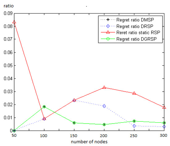
Figure 9.
Regret ratio of four methods (in generated network).
7. Conclusions and Future Work
In this paper, three main methods are proposed for the RTSP problem where the traveler finds the SP with minimized regret. In addition, the static RSP is also used as a comparison. The numerical result validates that the DGRSP and DMSP models, generally, have the best solution with less regret than the other two models. The Static RSP has the worst solution since it has not used the updated information. Although DRSP makes use of the updated information, it is generally not better than DGRSP and DMSP in most test cases. There are two reasons. First, DGRSP and DMSP models in stage t pay more attentions on the arcs near to the visitor-position for optimization, which makes full use of the updated information. Second, the DRSP problem is NP-hard, which leads to non-optimality for the large number nodes cases. The computation times of DGRSP and DMSP are all below 4 s, which is acceptable for real-time transportation route planning in reality. Unfortunately, the computation time of Static RSP and DRSP for more than 250 nodes may exceed 10 s, which is not so attractive for real-time applications.
The models also have a few limitations. For example, the DRSP model may not work well for large-scale problems and fast solution methods are appreciated. That is to say, developing more efficient models and algorithms for RTSP is a future research direction. In addition, the integration of the above methods in an application is also another research direction.
Author Contributions
Conceptualization, B.X.; methodology, B.X.; software, B.X.; validation, B.X., X.J. and Z.C.; formal analysis, B.X.; investigation, B.X.; resources, B.X.; data curation, B.X.; writing original draft preparation, B.X., X.J. and Z.C. All authors have read and agreed to the published version of the manuscript.
Funding
The work was partly supported by the National Natural Science Foundation of China, grant number 71571134, 71371141.
Data Availability Statement
The datasets analyzed during the current study are available in the repository link of https://weibo.com/3340591702/OrcGr5fYd (accessed on 19 November 2024).
Acknowledgments
The authors are deeply indebted to the editors, referees for their invaluable comments which greatly improve the presentation of this paper.
Conflicts of Interest
There are no conflicts of interest between the authors to be declared.
References
- Dijkstra, E.W. A note on two problems in connection with graphs. Numer. Math. 1959, 1, 269–271. [Google Scholar] [CrossRef]
- Floyd, R.W. Algorithm 97: Shortest path. Commun. Acm 1962, 5, 345. [Google Scholar] [CrossRef]
- Bellman, R.E. On a routing problem. Q. Appl. Math. 1958, 16, 87–90. [Google Scholar] [CrossRef]
- Ford, L.R., Jr.; Fulkerson, D.R. Flows in Networks; Princeton Univ. Press: Princeton, NJ, USA, 1962. [Google Scholar]
- Himmich, I.; El Hallaoui, I.; Soumis, F. A multiphase dynamic programming algorithm for the shortest path problem with resource constraints. Eur. J. Oper. Res. 2023, 315, 470–483. [Google Scholar] [CrossRef]
- Bahel, E.; Gomez-Rua, M.; Vidal-Puga, J. Stable and weakly additive cost sharing in shortest path problems. J. Math. Econ. 2024, 110, 102921. [Google Scholar] [CrossRef]
- Murchl, J.D. A Fixed Matrix Method for All Shortest Distances in a Directed Graph and for the Inverse Problem. Ph.D. Thesis, University of Karlsruhe, Karlsruhe, Germany, 1970. [Google Scholar]
- Dionne, R. Etude et extension d’un algorithme de Murchland. INFOR Inf. Syst. Oper. Res. 1978, 16, 132–146. [Google Scholar]
- Goto, S.; Sangiovanni-Vincentelli, A. A new shortest path updating algorithm. Networks 1978, 8, 341–372. [Google Scholar] [CrossRef]
- Ramalingam, G.; Reps, T. An incremental algorithm for a generalization of the shortest-path problem. J. Algorithms 1996, 21, 267–305. [Google Scholar] [CrossRef]
- Demetrescu, C.; Frigioni, D.; Marchetti-Spaccamela, A.; Nanni, U. Maintaining shortest paths in digraphs with arbitrary arc weights: An experimental study. In Proceedings of the Algorithm Engineering: 4th International Workshop, WAE 2000 Saarbrücken, Germany, September 5–8, 2000 Proceedings 4; Naher, S., Wagner, D., Eds.; Springer: Berlin/Heidelberg, Germany, 2000; Volume 1982, pp. 218–229. [Google Scholar]
- Buriol, L.S.; Resende, M.G.C.; Thorup, M. Speeding up dynamic shortest-path algorithms. INFORMS J. Comput. 2008, 20, 191–204. [Google Scholar] [CrossRef]
- Martin, J. Distribution of time through a directed acyclic network. Oper. Res. 1965, 13, 46–66. [Google Scholar] [CrossRef]
- Frank, H. Shortest paths in probabilistic graphs. Oper. Res. 1969, 17, 583–599. [Google Scholar] [CrossRef]
- Hassin, R.; Zemel, E. On shortest paths in graphs with random weights. Math. Oper. Res. 1985, 10, 557–564. [Google Scholar] [CrossRef]
- Mirchandani, P.B.; Soroush, H. Optimal paths in probabilistic networks: A case with temporary preferences. Comput. Oper. Res. 1985, 12, 365–381. [Google Scholar] [CrossRef]
- Mirchandani, P.B.; Soroush, H.; Angrealtta, G.; Mason, F.; Serafini, P. Routes and flows in stochastic networks. In Stochastics in Combinatorial Optimization; World Scientific Publishing Company: Singapore, 1986; pp. 129–177. [Google Scholar]
- Beigy, H.; Meybodi, M.R. A sampling method based on distributed learning automata for solving stochastic shortest path problem. Knowl.-Based Syst. 2021, 212, 106638. [Google Scholar] [CrossRef]
- Ketkov, S.S.; Prokopyev, O.A.; Burashnikov, E.P. An approach to the distributionally robust shortest path problem. Comput. Oper. Res. 2021, 130, 105212. [Google Scholar] [CrossRef]
- Lee, J.; Joung, S.; Lee, K. A fully polynomial time approximation scheme for the probability maximizing shortest path problem. Eur. J. Oper. Res. 2022, 300, 35–45. [Google Scholar] [CrossRef]
- Song, M.; Cheng, L. A generalized Benders decomposition approach for the mean-standard deviation shortest path problem. Transp. Lett. 2023, 15, 823–833. [Google Scholar] [CrossRef]
- Hall, R. The fastest path through a network with random time-dependent travel times. Transp. Sci. 1986, 20, 182–188. [Google Scholar] [CrossRef]
- Bertsimas, D.; Van Ryzin, G. A stochastic and dynamic vehicle routing problem in the Euclidean plane. Oper. Res. 1991, 39, 601–615. [Google Scholar] [CrossRef]
- Bertsimas, D.; Van Ryzin, G. Stochastic and dynamic vehicle routing in Euclidean plane with multiple capacitated vehicles. Oper. Res. 1993, 41, 60–76. [Google Scholar] [CrossRef]
- Psaraftis, H.; Tsitsiklis, J. Dynamic shortest paths in acyclic networks with Markovian arc costs. Oper. Res. 1993, 41, 91–101. [Google Scholar] [CrossRef]
- Azaron, A.; Kianfar, F. Dynamic shortest path in stochastic dynamic networks: Ship routing problem. Eur. J. Oper. Res. 2003, 144, 138–156. [Google Scholar] [CrossRef]
- Pattanamekar, P.; Park, D.; Rilett, L.R.; Lee, J.; Lee, C. Dynamic and stochastic shortest path in transportation networks with two components of travel time uncertainty. Transp. Res. Part C 2003, 11, 331–354. [Google Scholar] [CrossRef]
- Ojeda Rios, B.H.; Xavier, E.C.; Miyazawa, F.K.; Amorim, P.; Curcio, E.; Santos, M.J. Recent dynamic vehicle routing problems: A survey. Comput. Ind. Eng. 2021, 160, 107604. [Google Scholar] [CrossRef]
- Dias, L.C.; Climaco, J.N. Shortest path problems with partial information: Models and algorithms for detecting dominance. Eur. J. Oper. Res. 2000, 121, 16–31. [Google Scholar] [CrossRef][Green Version]
- Averbakh, I.; Lebedev, V. Interval data minmax regret network optimization problems. Discret. Appl. Math. 2004, 138, 289–301. [Google Scholar] [CrossRef]
- Zielinski, P. The computational complexity of the relative robust shortest path problem with interval data. Eur. J. Oper. Res. 2004, 158, 570–576. [Google Scholar] [CrossRef]
- Karasan, O.E.; Pinar, M.C.; Yaman, H. The Robust Shortest Path Problem with Interval Data; Bilkent University: Ankara, Turkey, 2001. [Google Scholar]
- Montemanni, R.; Gambardella, L.M.; Donati, A.V. A branch and bound algorithm for the robust shortest path problem with interval data. Oper. Res. Lett. 2004, 3, 225–232. [Google Scholar] [CrossRef]
- Montemanni, R.; Gambardella, L.M. The robust shortest path problem with interval data via Benders decomposition. 4OR 2005, 3, 315–328. [Google Scholar] [CrossRef]
- Kasperski, A.; Zielinski, P. An approximation algorithm for interval data minimax regret combinatorial optimization problems. Inf. Process. Lett. 2006, 97, 177–180. [Google Scholar] [CrossRef]
- Catanzaro, D.; Labbe, M.; Salazar-Neumann, M. Reduction approaches for robust shortest path problems. Comput. Oper. Res. 2004, 38, 1610–1619. [Google Scholar] [CrossRef]
- Chassein, A.; Dokka, T.; Goerigk, M. Algorithms and uncertainty sets for data-driven robust shortest path problems. Eur. J. Oper. Res. 2019, 274, 671–686. [Google Scholar] [CrossRef]
- Zhang, C. Problem characterization of unique shortest path routing. Comput. Ind. Eng. 2023, 178, 109110. [Google Scholar] [CrossRef]
- Davoodi, M.; Ghaffari, M. Shortest path problem on uncertain networks: An efficient two phases approach. Comput. Ind. Eng. 2021, 157, 107302. [Google Scholar] [CrossRef]
- Xu, B.; Zhou, X. Dynamic relative robust shortest path problem. Comput. Ind. Eng. 2020, 148, 106651. [Google Scholar] [CrossRef]


Disclaimer/Publisher’s Note: The statements, opinions and data contained in all publications are solely those of the individual author(s) and contributor(s) and not of MDPI and/or the editor(s). MDPI and/or the editor(s) disclaim responsibility for any injury to people or property resulting from any ideas, methods, instructions or products referred to in the content. |
© 2025 by the authors. Licensee MDPI, Basel, Switzerland. This article is an open access article distributed under the terms and conditions of the Creative Commons Attribution (CC BY) license (https://creativecommons.org/licenses/by/4.0/).