Disturbance Observer-Based Dynamic Surface Control for Servomechanisms with Prescribed Tracking Performance

Abstract

The critical design challenge for a class of servomechanisms is to reject unknown dynamics (including internal uncertainties and external disturbances) and achieve the prescribed performance of the tracking error. To get rid of the influence of unknown dynamics, an extended state observer (ESO) is employed to estimate system states and total unknown dynamics and does not require a priori information of the known dynamic. Meanwhile, an improved prescribed performance function is presented to guarantee the transient performance of the tracking error (e.g., the overshoot, convergence rate, and the steady state error). Consequently, a modified dynamic surface control strategy is designed based on the estimations of the ESO and error constraints. The stability of the proposed control strategy is demonstrated using Lyapunov theory. Finally, some simulation results based on a turntable servomechanism show that the proposed method is effective, and it has a better control effect and stronger anti-disturbance ability compared with the traditional control method.

1. Introduction

At present, servomechanisms are mainly classified as hydraulic servo control systems, electromechanical servo systems (including AC servo control systems and DC servo control systems), and pneumatic servo systems based on the executive component. Thereinto, because of their excellent performance, fast response, low speed, high torque, good linearity, low torque fluctuation, and simple and compact structure, electromechanical servo control systems executed using a servomotor are extensively used in military systems, civilian industrial control systems, and the robot industry to implement highly precise motion control [1,2,3]. Moreover, from the perspective of control, the servomotor is a single variable control system; thus, both the classical control theory and modern control theory are suitable for this system. Therefore, the servomotor control system plays an important role in motion control systems and has a great value for research. With its wide applications, the requirements for servomotor control become higher in major fields. However, the servomotor is a nonlinear strong coupling controlled object that encounters parameter uncertainties, load disturbances, fraction disturbances, and measurement noises. Thus, the goal of the servomotor control system design is to realize high-precision tracking and good anti-disturbance ability.

In traditional control methods, the conventional PI/PID controller is usually adopted, with a structure that is simple and parameters that are easy to be set. Nevertheless, it does not meet the criteria for high-accuracy and high-speed positioning applications [4,5,6]. Therefore, many modern control methods are presented to improve the control effect, such as intelligent control, sliding mode control (SMC), adaptive robust control (ARC), and $H\infty$ control [7,8,9,10,11,12,13,14,15,16,17]. In other systems, estimation and observer techniques are used as a novel strategy to estimate unknown state variables, and these methods been implemented in some motion control systems. In [18,19], the authors proposed a disturbance observer based on control (DOBC) method to compensate for the external uncertainties. In [20], the authors proposed a modified fuzzy Luenberger observer. However, the aforementioned methods usually are based on an accurate mathematical model or the reconstruction of external disturbances. In practice, these disturbances (including internal uncertainties, external disturbances, and measurement noises) can affect the performance of the control system, and they are difficult to measure. To solve this problem, dynamic surface control was designed by introducing a first-order filter at each step of backstepping method, which has improved the performance of the backstepping method [21]. This method assumes that the unknown nonlinear dynamics are linearly parameterized. The aforementioned methods cannot prescribe transient performance (e.g., overshoot, convergence rate, and steady state error). Therefore, more effective approaches to achieve higher motion precision against uncertainties are still pursued in practice.

Based on the above analysis, the extended state observer (ESO) proposed by Han [22] is employed in this paper. This method has been employed in many new control methods [23,24,25,26,27] and has achieved some improvements in the performance of the control system with uncertainties. It is used to estimate system states and unknown dynamics (including frictions, parameter uncertainties, load disturbances, and external disturbances) by lumping all unknown dynamics into an extended state variable, which does not need accurate information about these unknown dynamics. Then, these estimations are incorporated into the controller design. Additionally, an improved prescribed performance function with error constraints is employed to achieve the expected transient performance. Therefore, this paper proposes a novel dynamic surface control strategy with the prescribed performance function based on an ESO for nonlinear servomechanisms to improve performance. Finally, comparative simulations based on a turntable servo system are provided to validate the efficacy of the proposed method.

The main contributions of this paper are summarized as follows:

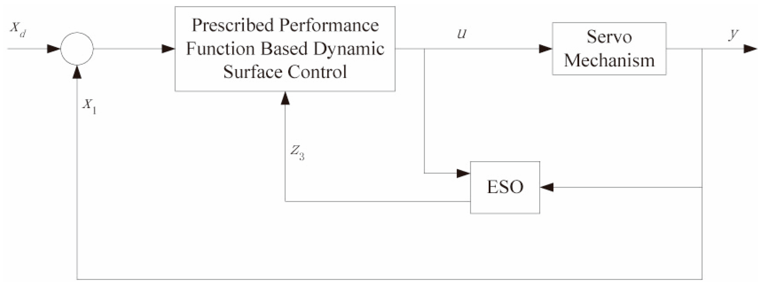
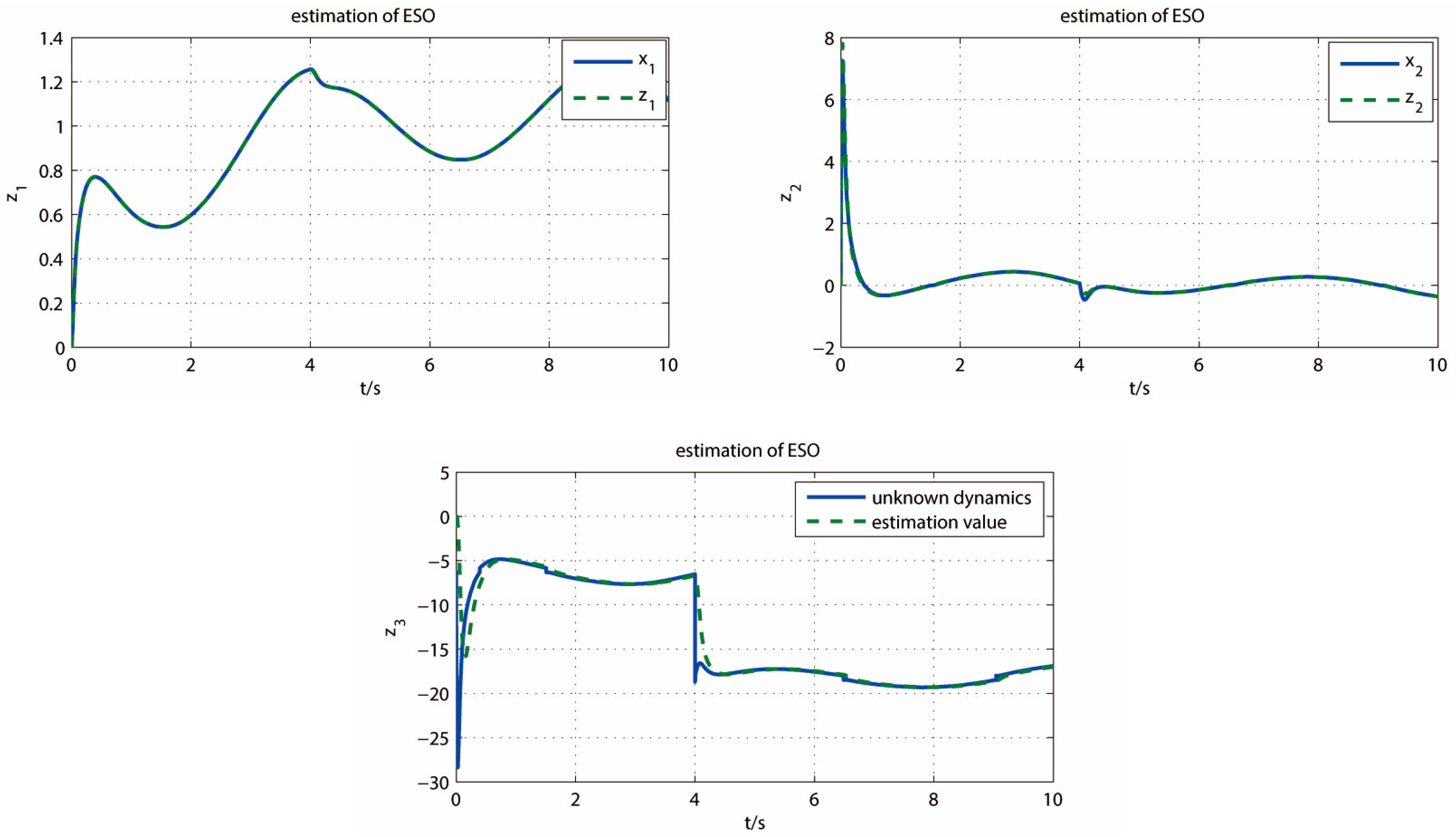
• Frictions, parameter uncertainties, load disturbances, and external disturbances are lumped as an extended state variable, which is estimated using an ESO and compensated in the controller. It solves the requirement for linear parameterization of the unknown nonlinear dynamics in the traditional dynamic surface control and improves the anti-disturbance ability. Furthermore, the parameters of the ESO are designed based on the observer bandwidth only to simplify the parameter tuning;
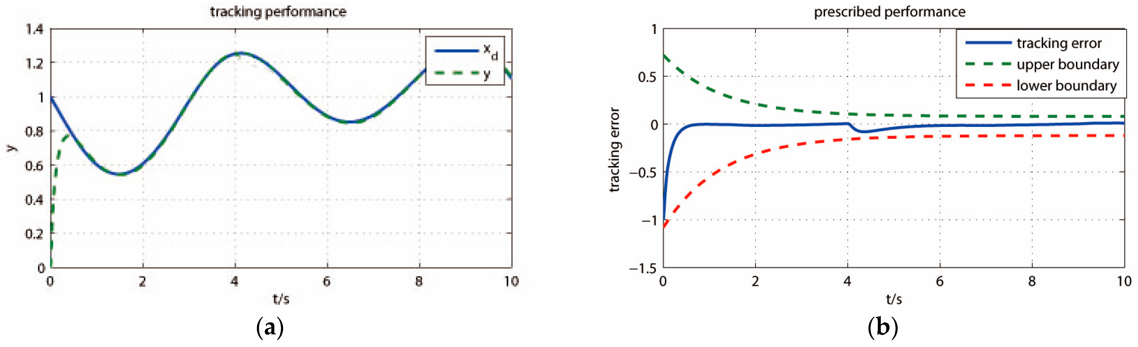
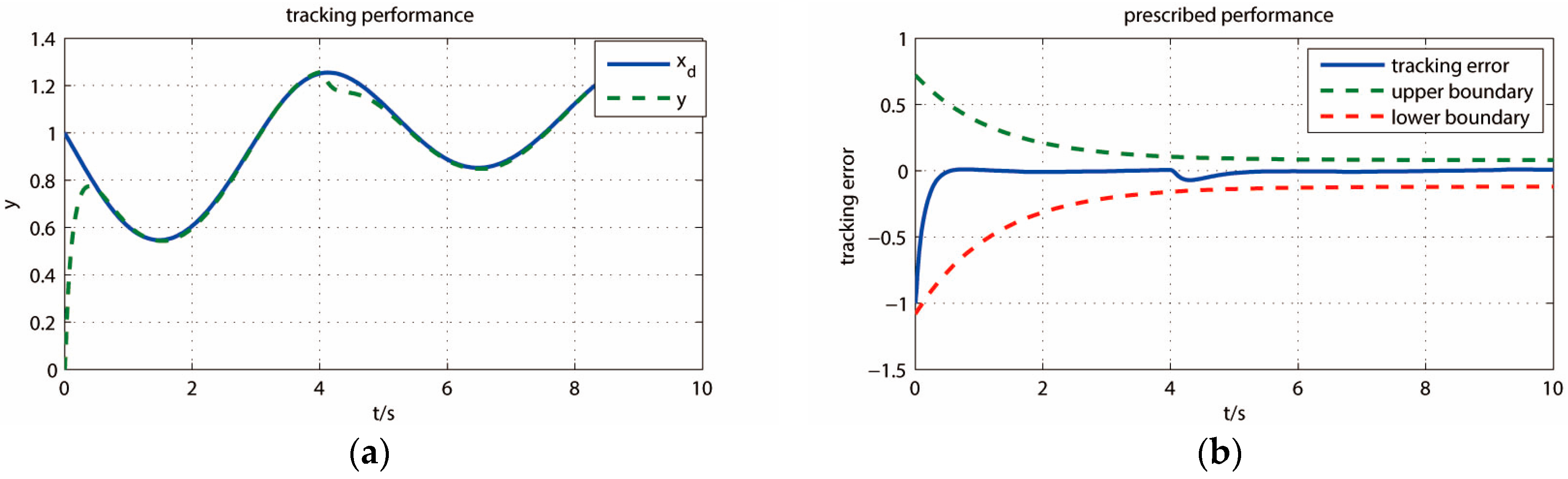
• A prescribed performance function is employed to achieve the expected transient performance. It is incorporated into the controller design to ensure the tracking error within a prescribed region;
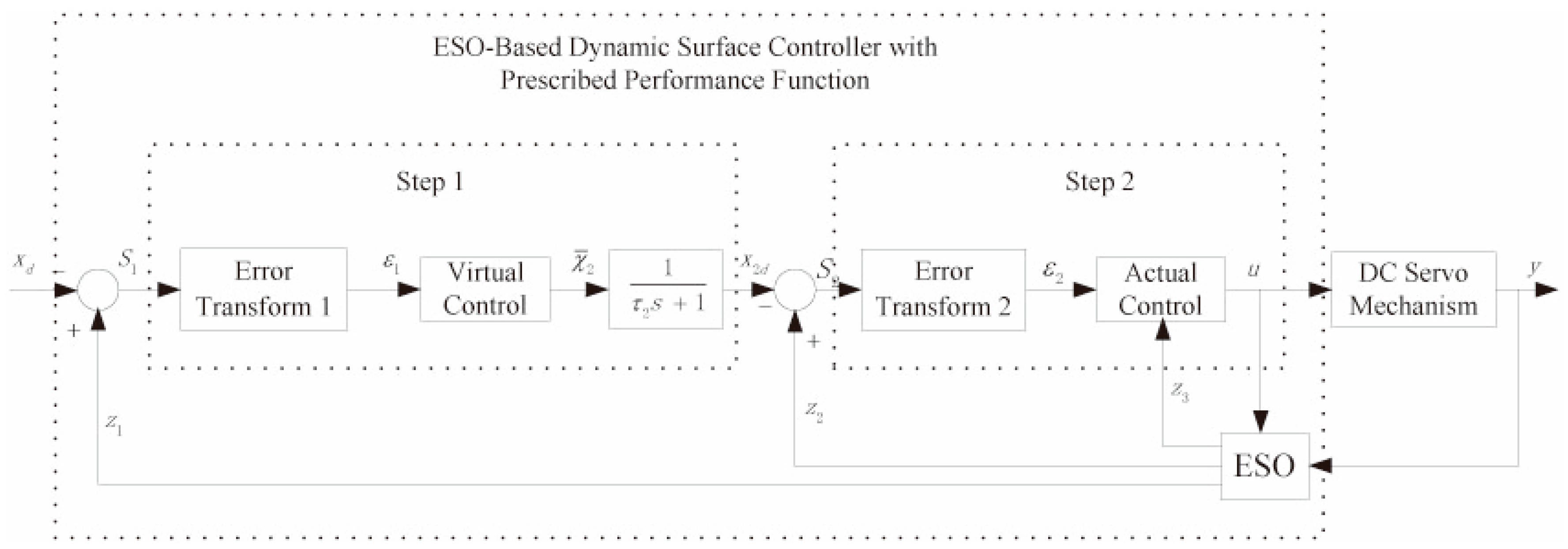
• A novel dynamic surface control combined with the prescribed performance function and an ESO is proposed for a turntable servo system with many unknown disturbances. It fully takes advantage of the low computational complexity of the dynamic surface control and improves the control performance of the control system;
• Furthermore, the conclusion is drawn using Lyapunov theory. Specifically, the proposed design is uniformly ultimately bounded, all signals of the closed-loop control system are bounded, and the estimate error of the ESO and tracking error of the design converge to a small neighborhood around the equilibrium point.

The remainder of this paper is organized as follows. The dynamic model of the servomechanism and the problem statement are given in Section 2. Section 3 designs the ESO and the prescribed performance function, and then presents a novel dynamic surface control strategy, combining the estimated unknown dynamics via the ESO with the prescribed performance function. Section 4 analyzes the stability of the proposed control strategy based on Lyapunov theory. Some numerical simulations are discussed in Section 5. Section 6 gives concluding remarks.

2. Dynamic Model and Problem Description

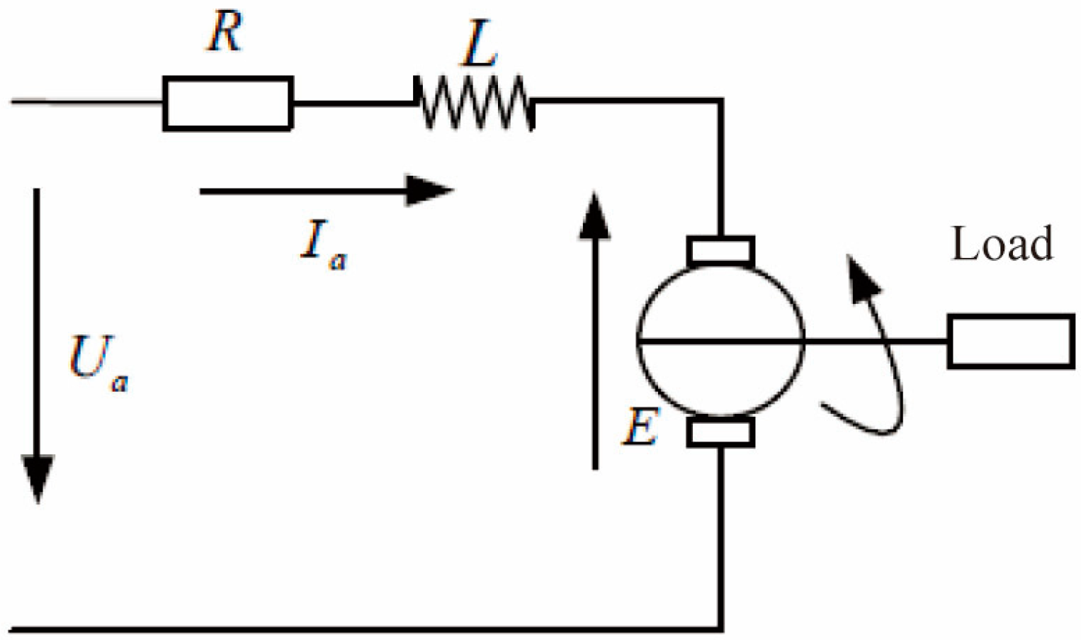
This section mainly develops the dynamic model and describes the control problem in order to design an effective control system.

2.1. Dynamic Model

This paper considers a turntable servomechanism driven by two permanent magnet DC motors. It is a high-precision servo control component, and its technical index parameters are shown in

Table 1. Technical index parameters of the motors.

Motor Type	Azimuth Motor: 200LYX25-DS
Armature voltage	28 V
Armature resistance	2.6 Ω
Armature inductance	5.4 mH
Maximum non-load speed	186 r/m
Moment of inertia	1645.866 × 10–5 kg·m2
Motor torque coefficient	1.24 N·m/A

(Note: this paper selects the azimuth axis as the control objective).

The equivalent circuit of the permanent magnet DC motor with load is shown in Figure 1.

According to Kirchhoff Voltage Law (KVL), the voltage balance equation of the armature circuit is given as follows:

$$U_a=R_a{I}_a+L{\displaystyle \frac{d{I}_a}{dt}}+E$$

(1)

where

Ua—applied d-c voltage, volts/V;

Ia—armature current, amperes/A;

Ra—armature resistance, ohms/Ω;

L—armature inductance, henrys/H;

E—the back electromotive force, volts/V, $E=K_B\cdot {\displaystyle \frac{d\theta }{dt}}$;

$K_B$—motor emf constant, volts per radian per second;

$\theta$—angular position of the motor shaft, radians.

The torque balance equation of the motor is given as follows:

$$T_a=T_m+T_f+T_l+T_d$$

(2)

where

$T_a$—motor electromagnetic torque, $T_a=K_T\cdot I_a$;

$K_T$—motor torque constant, pound-feet per ampere;

$T_m$—motor inertia torque, $T_m=J\cdot {\displaystyle \frac{d{\omega }_L}{dt}}=J\cdot {\displaystyle \frac{d{\theta }^2}{d{t}^2}}$;

J—equivalent moment of inertia of motor, gears and load referred to the motor shaft, kg·m²;

$T_f$—motor friction torque;

$T_l$—motor load torque;

$T_d$—motor disturbance torque.

Then the dynamic model of the DC servomechanism is given as follows:

$$\left\{\begin{array}{c}L{\displaystyle \frac{d{I}_a}{dt}}=U_a-R_a{I}_a-K_B{\displaystyle \frac{d\theta }{dt}}\\ J{\displaystyle \frac{d^2\theta }{d{t}^2}}=K_T{I}_a-\left(T_f+T_l+T_d\right)\end{array}\right.$$

(3)

The electrical time constant $L/R_a$ is much smaller than the mechanical time constant in practice. Therefore, from Equation (3), we know that the electrical transients decay very rapidly, and $L(d{I}_a/dt)$ is very close to zero [28]. Thus, the dynamic model of the servomechanism is simplified as follows:

$${\displaystyle \frac{d^2\theta }{d{t}^2}}={\displaystyle \frac{K_T}{R_{a}J}}{U}_a-{\displaystyle \frac{K_T{K}_B}{R_{a}J}}{\displaystyle \frac{d\theta }{dt}}-{\displaystyle \frac{\left(T_f+T_l+T_d\right)}{J}}$$

(4)

Here, it defines the output angular position and the angular velocity as state variables, i.e., ${[x_1, x_2]}^T={[\theta , \stackrel{•}{\theta }]}^T$, and defines the output angular position $\theta$ as the system output, i.e., $\mathrm{y}=\theta =x_1$. Meanwhile, defining $K_1={\displaystyle \frac{K_T}{R_a}}$, $K_2={\displaystyle \frac{K_T{K}_B}{R_a}}$, and $\mathrm{u}=U_{\mathrm{a}}$ (as the control inputs) from the dynamic model Equation (4), the state space form is given as follows:

$$\left\{\begin{array}{c}{\dot{x}}_1=x_2\\ {\dot{x}}_2=-{\displaystyle \frac{K_2}{J}}{x}_2+{\displaystyle \frac{K_1}{J}}u-{\displaystyle \frac{T_f+T_l+T_d}{J}}\\ y=x_1\end{array}\right.$$

(5)

2.2. Problem Description

The researched servomechanism in this paper is applied to the ship-borne photoelectric tracking system. Thus, to get rid of the influence of the ship movement and obtain the stable tracking, first, coordinate transformation technology is used to conduct the real-time compensation of the attitude angle caused by ship swaying.

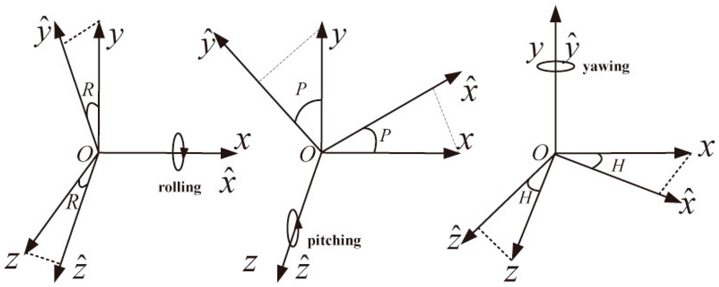
2.2.1. Coordinate Transformation

The attitude of the turntable is measured using the optical encoder based on the deck coordinate system. The optoelectronic target is based on the geographic coordinate system. Thus, it is extremely necessary to convert the data between deck coordinates and geographic coordinates [29], as shown in Figure 2.

First, we consider the movement of each axis separately, as shown in Figure 3.

(1) For the rolling, the coordinate is given as follows:

$$\left[\begin{array}{c}\widehat{x}\\ \widehat{y}\\ \widehat{z}\end{array}\right]=\left[\begin{array}{ccc}1& 0& 0\\ 0& \cos R& \sin R\\ 0& -\sin R& \cos R\end{array}\right]\left[\begin{array}{c}x\\ y\\ z\end{array}\right]$$

(6)

(2) For the pitching, the coordinate is given as follows:

$$\left[\begin{array}{c}\widehat{x}\\ \widehat{y}\\ \widehat{z}\end{array}\right]=\left[\begin{array}{ccc}\cos P& \sin P& 0\\ -\sin p& \cos P& 0\\ 0& 0& 1\end{array}\right]\left[\begin{array}{c}x\\ y\\ z\end{array}\right]$$

(7)

(3) For the yawing, the coordinate is given as follows:

$$\left[\begin{array}{c}\widehat{x}\\ \widehat{y}\\ \widehat{z}\end{array}\right]=\left[\begin{array}{ccc}\cos H& 0& \sin H\\ 0& 1& 0\\ -\sin H& 0& \cos H\end{array}\right]\left[\begin{array}{c}x\\ y\\ z\end{array}\right]$$

(8)

Then, by integrating three axis movements, we can obtain the coordinate transformation formula as follows:

$$\left[\begin{array}{c}{x}_c\\ y_c\\ z_c\end{array}\right]=\left[\begin{array}{ccc}1& 0& 0\\ 0& \cos R& \sin R\\ 0& -\sin R& \cos R\end{array}\right]\left[\begin{array}{ccc}\cos P& \sin P& 0\\ -\sin p& \cos P& 0\\ 0& 0& 1\end{array}\right]\left[\begin{array}{ccc}\cos H& 0& \sin H\\ 0& 1& 0\\ -\sin H& 0& \cos H\end{array}\right]\left[\begin{array}{c}x\\ y\\ z\end{array}\right]$$

(9)

where $x_c$, $y_c$, and $z_c$ are the deck coordinate system; and $x$, $y$, and $z$ are the geographic coordinate system.

According to Figure 2b, one can obtain the azimuth and pitch:

$$A_c=\arctan z_c/x_c, E_c=\arcsin y_c/D$$

(10)

Then, by combing with (9), the azimuth angle $A_c$ and the pitch angle $E_c$ are respectively obtained as follows:

$$\begin{array}{ll}\hfill A_c& ={\tan }^{-1}\left\{\right\{\cos E(\cos R\sin (A-H)+\sin R\sin P\cos (A-H))\\ & -\sin E\sin R\cos P\}/\{\cos E\cos P\cos (a-h)+\sin E\sin p\left\}\right\}\end{array}$$

(11)

$$\begin{array}{ll}\hfill E_c& ={\sin }^{-1}\{\cos E(\sin R\sin (A-H)-\cos R\sin P\cos (A-H)\\ & +\sin E\cos R\cos P\}\end{array}$$

(12)

where the heeling angle R is the diversion of the ship around the fore-and-aft line relative to horizontal level; the trimming angle P is the angle of the fore-and-aft line relative to the horizontal; and the heading angle H is the angle between the projection of fore-and-aft line in the horizontal and the north line. A and E are the azimuth angle and pith angle in the geographic coordinate system, respectively.

Therefore, Equations (11) and (12) are the reference signals of the azimuth axis and the pitch axis, respectively. They can compensate for the influence caused by ship movement.

2.2.2. Problem Description

In practice, parameters of the system may possess some perturbations. From Equation (5), we observer that the parameter perturbation and some additive measurement noises on the state variables ($x_1, x_2$) can be lumped into the term $T_d$. Thus, $-{\displaystyle \frac{T_f+T_l+T_d}{J}}$ can be regarded as the total disturbance term (including internal disturbances and external disturbances).

Assumption 1. 

The total disturbance term in Equation (5) is differentiable, and the differential is bounded, i.e., ${‖-{\displaystyle \frac{T_f+T_l+T_d}{J}}‖}^{\prime }\le \delta$, where $\delta$ is a positive constant.

This assumption is practically feasible in servo systems and thus has been widely recognized in ESO studies (see [30] and references therein).

Assumption 2. 

The given reference trajectory $x_d$ is continuous and bounded, and its first-order derivative ${\dot{x}}_d$ is available and bounded.

The control problem of this paper is stated as follows: It synthesizes an appropriate feedback control u such that the output angular position $y=x_1$ tracks the given reference trajectory $x_d$ as closely as possible in the face of multiple disturbances. Meanwhile, the tracking error is always guaranteed in a prescribed range.

3. Control Strategy

This paper focus on the disturbance rejection problem of the servomechanism (5). We mainly address the dynamic surface control design of the ESO-based composite control law for the position control of the servomechanism with error constraints. First, an ESO is employed to estimate the total disturbances and the state variables. Then, the prescribed performance function is described. Finally, the novel dynamic surface control is designed using the estimate dynamics and the error constraints.

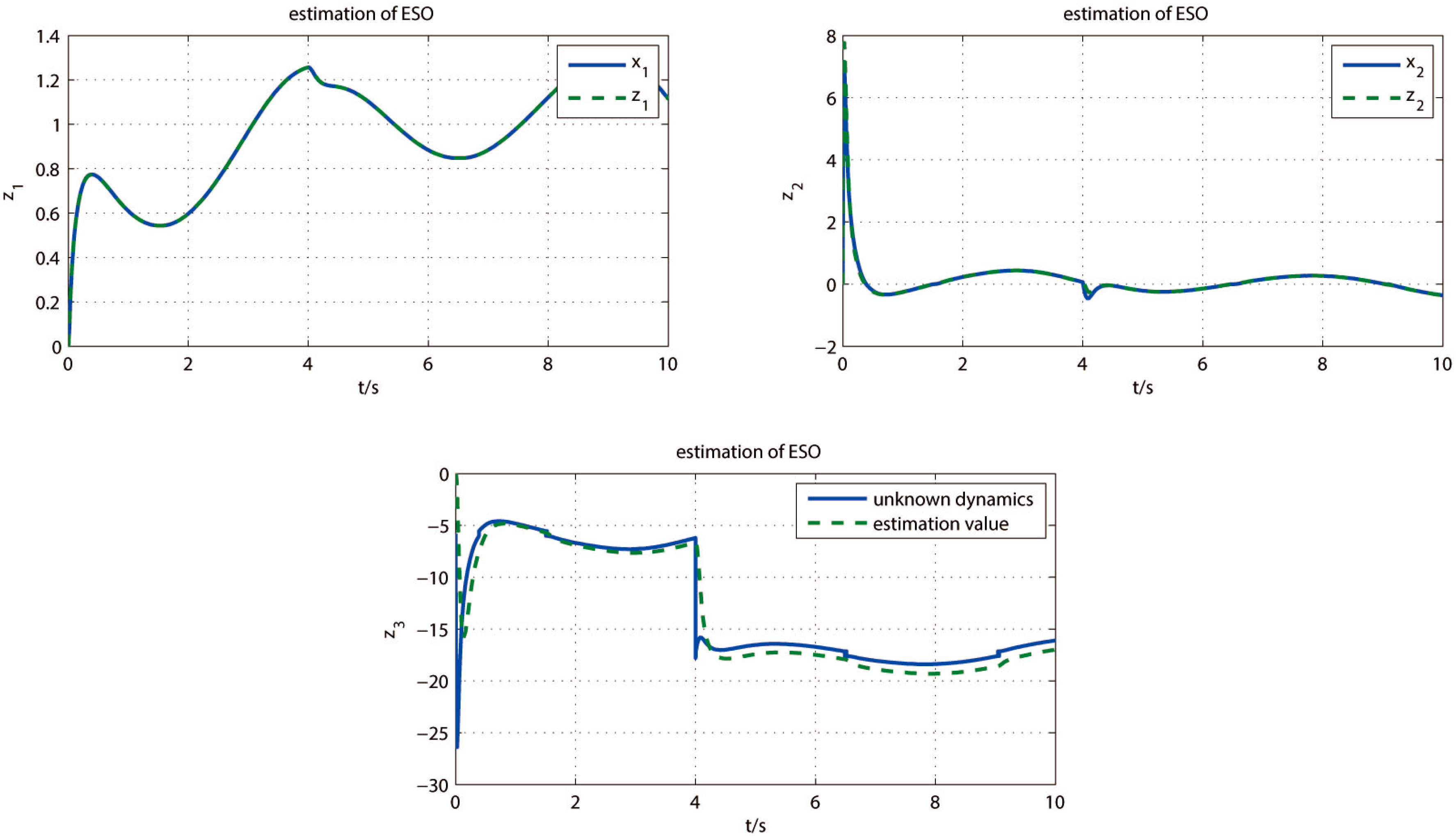
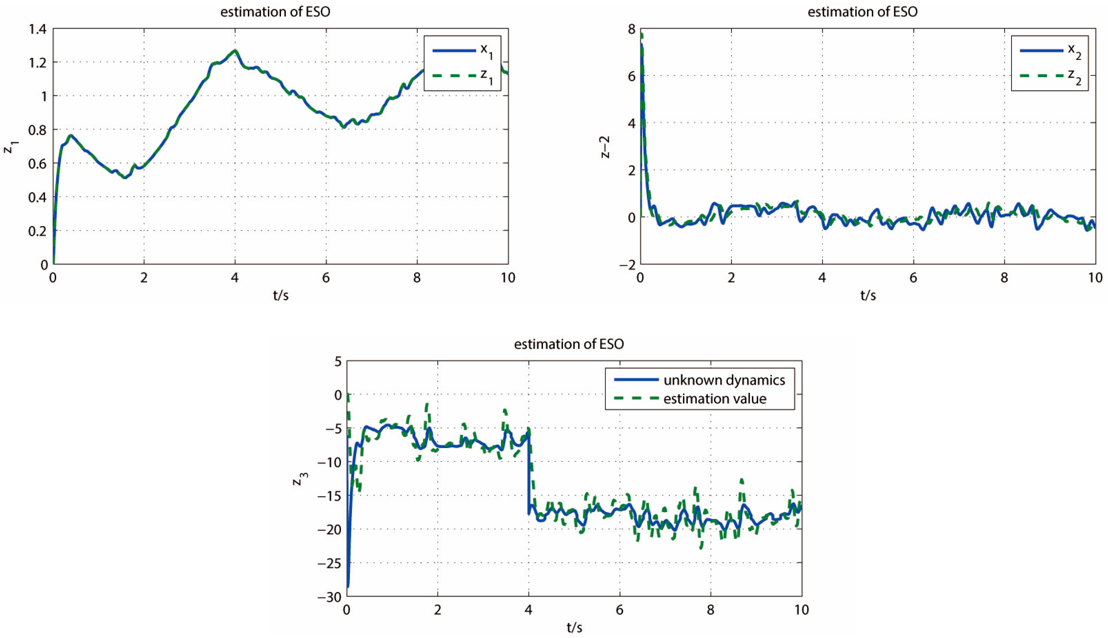
3.1. Extended State Observer Design

According to the analysis in Section 2.2, the parameters perturbation, measurement noise, fraction disturbances, load disturbances, and external disturbances can be lumped into a total disturbance term, which will be estimated by the ESO and then compensated for in the controller design.

In order to estimate the total disturbance using the ESO, we first define the lumped unknown dynamics as an extended state variable, i.e., $x_3=-{\displaystyle \frac{T_f+T_l+T_d}{J}}$. Then, state variables of system Equation (5) can be augmented to $x=[x_1, x_2, x_3]$. Defining the time derivative of $x_3$ as $h(t)$, we can obtain the extended state space form of the original system (5) as follows:

$$\left\{\begin{array}{c}{\dot{x}}_1=x_2\\ {\dot{x}}_2=-{\displaystyle \frac{K_2}{J}}{x}_2+{\displaystyle \frac{K_1}{J}}u+x_3\\ {\dot{x}}_3=h\left(t\right)\\ y=x_1\end{array}\right.$$

(13)

The unknown dynamics will degrade the performance of the closed-loop control. Thus, they must be estimated and compensated for in the controller design. To better solve the problem, an ESO is designed to estimate state variables and the lumped known dynamics, which can be compensated for in the controller.

First, the observability matrix of the extended state space from Equation (13) is full rank, i.e., $rank([C, CA, C{A}^2]=3$; thus, the extended system Equation (13) is observable.

Then, in order to reduce controller parameters, a linear ESO is designed in this section. According to [30], the linear ESO is given as follows:

$$\left\{\begin{array}{c}{\dot{z}}_1=z_2+{\beta }_1\left(y-z_1\right)\\ {\dot{z}}_2=-{\displaystyle \frac{K_2}{J}}{x}_2+z_3+{\beta }_2\left(y-z_1\right)+{\displaystyle \frac{K_1}{J}}u\\ {\dot{z}}_3={\beta }_3\left(y-z_1\right)\end{array}\right.$$

(14)

where $z_1, z_2, z_3$ are estimated values of system states and the total disturbance, respectively; and ${\beta }_1, {\beta }_2, {\beta }_3$ are parameters of the ESO. The parameters of the ESO (14) can be set as follows: ${\beta }_1=3{\omega }_e, {\beta }_2=3{{\omega }_e}^2, {\beta }_3={{\omega }_e}^3, {\omega }_e>0$, where ${\omega }_e$ represents the bandwidth of the ESO [31].

In order to design a controller using the observer variables, the convergence of the ESO must be analyzed first. Defining the observer error of ESO as $e_i=x_i-z_i, i=1, 2, 3$ and combing Equations (13) and (14), the observer error dynamic is given as follows:

$$\left\{\begin{array}{c}{\dot{e}}_1=e_2-3{\omega }_e{e}_1\\ {\dot{e}}_2=e_3-3{{\omega }_e}^2{e}_1\\ {\dot{e}}_3=h\left(t\right)-{{\omega }_e}^3{e}_1\end{array}\right.$$

(15)

According to [30], transforming the observer error using ${\epsilon }_i=e_i/{{\omega }_e}^{i-1}, i=1, 2, 3$, Equation (15) can be rewritten as follows:

$$\dot{\epsilon }={\omega }_e{A}_e\epsilon +M_e{\displaystyle \frac{h\left(t\right)}{{{\omega }_e}^2}}$$

(16)

where $A_e=\left[\begin{array}{ccc}-3& 1& 0\\ -3& 0& 1\\ -1& 0& 0\end{array}\right]$, $A_e$ is Hurwitz, and $M_e=\left[\begin{array}{c}0\\ 0\\ 1\end{array}\right]$. Then, the linear nominal system of the observer error system outline in Equation (15) is given as follows:

$$\dot{\epsilon }={\omega }_e{A}_e\epsilon$$

(17)

For $A_e$ is Hurwitz and ${\omega }_e>0$, one can find a positive definite matrix P, which is the solution of $P\ast A_e+{A_e}^T\ast P=-I$, so that $V={\epsilon }^{T}P\epsilon >0, \dot{V}=-{\omega }_e{\epsilon }^T\epsilon <0$. Thus, the observer error system is uniformly asymptotically stable (exponentially stable) [30,31]. The detailed proof can be obtained following the analysis in [30,31]; thus, it will not be presented due to space limitations.

Remark 1. 

When the observer is stable, the derivative of vector $\dot{e}=0$. Then, the observer error can be written as follows:

$$\left\{\begin{array}{c}{e}_2=3{\omega }_e{e}_1={\displaystyle \frac{3}{{{\omega }_e}^2}}h\left(t\right)\\ e_3=3{{\omega }_e}^2{e}_2={\displaystyle \frac{3}{{\omega }_o}}h\left(t\right)\\ e_1={\displaystyle \frac{h\left(t\right)}{{{\omega }_e}^3}}\end{array}\right.$$

(18)

Thus, observer errors are determined by the bandwidth ${\omega }_e$ of the ESO. By tuning the parameter appropriately, observer errors can be forced to a sufficiently small constant such that $z_i$ can converge into a neighborhood of the actual states $x_i$. Furthermore, ${\omega }_e$ can be selected to be large enough such that $e_i$ is small although h(t) is unknown. However, a very large ${\omega }_e$ may reduce the robustness of the proposed ESO and cause high-frequency oscillations due to the induced high-gain integration. Therefore, to solve this problem, Chen [32] proposed a novel parameter tuning method, i.e., ${\beta }_1=3{\omega }_e, {\beta }_2=3{{\omega }_e}^2, {\beta }_3=k{\beta }_2$ (the detailed analysis is presented in [32]).

Remark 2. 

The parameters of the ESO are very important and determines the stability of the observer. In practical situation, the state observer provides information on the internal states of the plants that are unavailable. They are also used as noise filters. Therefore, the bandwidth ${\omega }_e$ needs to be chosen appropriately.

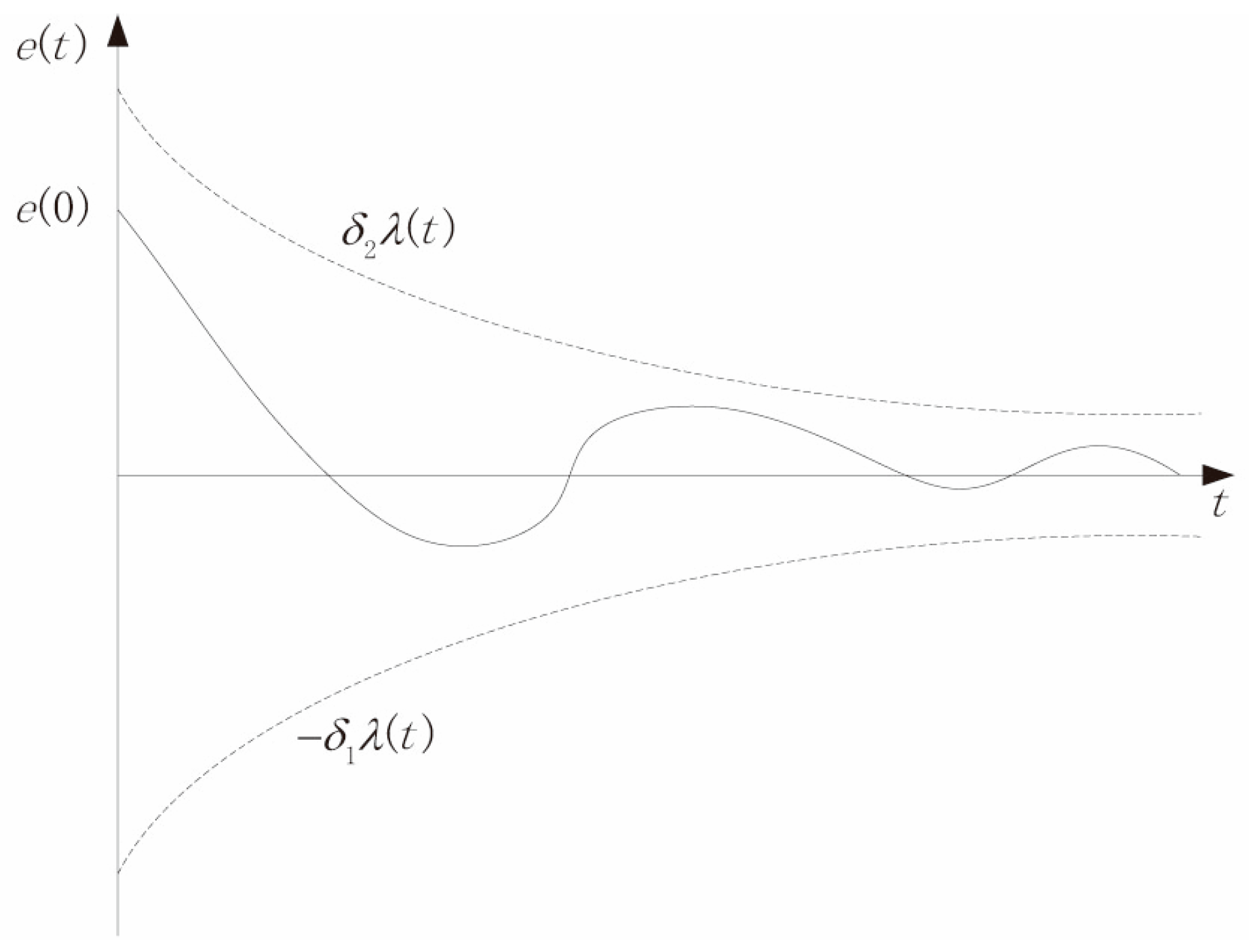
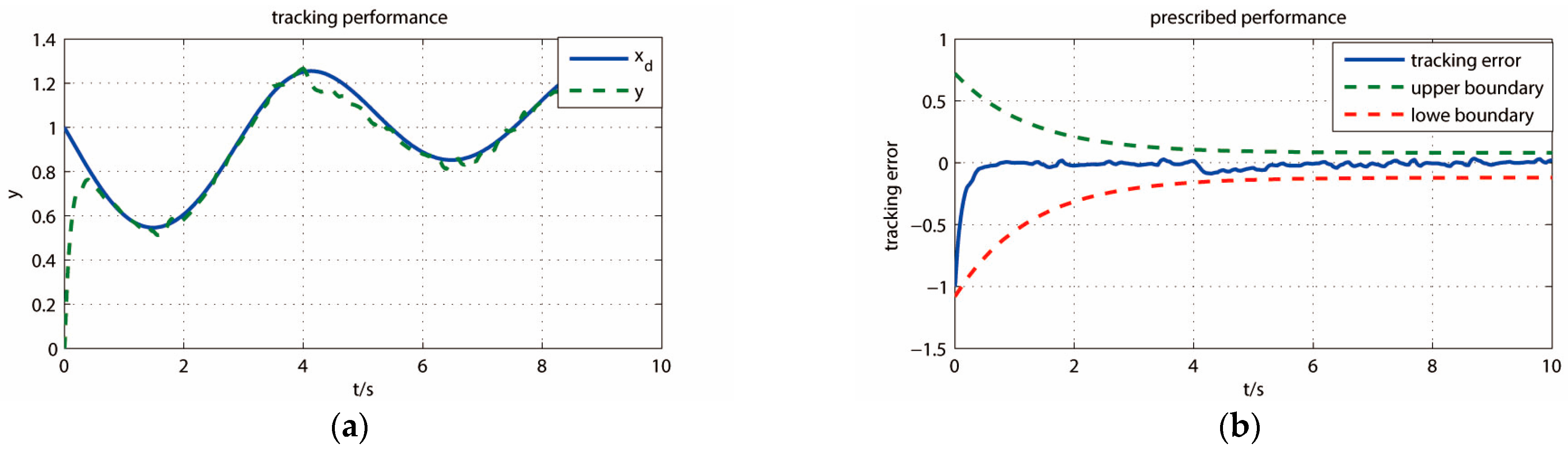
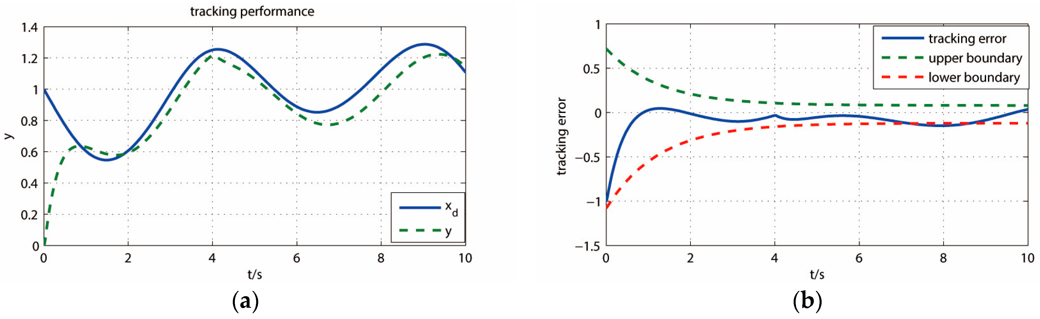
3.2. Prescribed Performance Control

In order to guarantee the transient performance of the closed-loop system (e.g., the overshoot, the convergence rate, and the steady state error), a prescribed performance control strategy is proposed in this section. Then, it is used to design the controller so that the tracking error of the closed-loop system can be restrained in a predefined trajectory.

According to [33], defining the tracking error $e(t)$, the prescribed performance function $\lambda (t)$: $R^{+}\to R^{-}$ is given as follows:

$$\lambda \left(t\right)=\left({\lambda }_0-{\lambda }_{\infty }\right)e^{-ct}+{\lambda }_{\infty }$$

(19)

where $Li{m}_{t\to \infty }\lambda (t)={\lambda }_{\infty }>0$; $c$ is the convergence rate of tracking error and is a positive constant; and ${\lambda }_0>{\lambda }_{\infty }$. It is a positive decreasing smooth function, and ${\lambda }_0$, ${\lambda }_{\infty }$, and $c$ are the design parameters.

In order to simplify prescribed performance function, as presented in [34], the prescribed performance can be obtained if condition (20) holds as follows:

$$-{\delta }_1\lambda \left(t\right)<e\left(t\right)<{\delta }_2\lambda \left(t\right),\forall >0$$

(20)

where ${\delta }_1$ and ${\delta }_2$ are positive constants, as shown in Figure 4.

From Equations (19) and (20), $-{\delta }_1\lambda (0)$ is the lower bounded of the undershoot, and ${\delta }_2\lambda (0)$ is the upper bound of the maximum overshoot. Thus, we can achieve the prescribed performance (including the transient and steady-state process) by tuning the parameters of ${\delta }_1$, ${\delta }_2$, ${\lambda }_0$, ${\lambda }_{\infty }$, and $c$. This is clearly illustrated in Figure 4.

In order to implement the control objective, the prescribed performance Equation (20) is usually transformed into an equivalent form with no constraints. Defining an output error transform $f(\epsilon )$ of the transformed error $\epsilon \in R$, it satisfies the following conditions:

(1)

It is a smooth strictly increasing function;

(2)

$-{\delta }_1<f(\epsilon )<{\delta }_2,{\forall }_{\epsilon }\in L_{\infty }$;

(3)

$Li{m}_{\epsilon \to +\infty }f(\epsilon )={\delta }_2$ and $Li{m}_{\epsilon \to -\infty }f(\epsilon )=-{\delta }_1$.

Then, the tracking error is written as follows:

$$e\left(t\right)=f\left(\epsilon \right)\lambda \left(t\right)$$

(21)

For $\lambda (t)>0$, the following can be deduced:

$$\epsilon =f^{-1}\left({\displaystyle \frac{e\left(t\right)}{\lambda \left(t\right)}}\right)$$

(22)

Remark 3. 

Selecting appropriate parameters of Equations (19) and (20), it can guarantee $-{\delta }_1\lambda (0)<e(0)<{\delta }_2\lambda (0)$. If the transform error $\epsilon$ is bounded, then $-{\delta }_1\lambda (t)<e(t)<{\delta }_2\lambda (t)$ can be guaranteed. Therefore, this transformation is effective and can be used as the prescribed performance function.

This paper employs a function possessing all required properties [34]:

$$f\left(\epsilon \right)={\displaystyle \frac{{\delta }_2{e}^{\epsilon }-{\delta }_1{e}^{-\epsilon }}{e^{\epsilon }+e^{-\epsilon }}}$$

(23)

It satisfies the above conditions, then the transformed error is deduced as follows:

$$\epsilon =f^{-1}\left({\displaystyle \frac{e\left(t\right)}{\lambda \left(t\right)}}\right)={\displaystyle \frac{1}{2}}\ln \left({\displaystyle \frac{e\left(t\right)}{\lambda \left(t\right)}}+{\delta }_1\right)-{\displaystyle \frac{1}{2}}\ln \left({\delta }_2-{\displaystyle \frac{e\left(t\right)}{\lambda \left(t\right)}}\right)$$

(24)

Thus, the stabilization of transformed error dynamics $\epsilon$ is sufficient to guarantee the tracking control of the system in Equation (5) with the prescribed error performance as given in Equation (20). In following section, this function will be employed to design the controller such that it achieves the prescribed performance.

3.3. Controller Design

In this section, a novel dynamic surface control based on an ESO [Equation (14)] and transformed error dynamics [Equation (24)] is proposed for the system [Equation (5)], as shown in Figure 5.

In traditional dynamic surface control method, only the tracking error is used to design the control law. As a result, it cannot guarantee the tracking error region of the transient process [35]. In addition, the traditional dynamic surface control requires that the unknown dynamics be linearly parameterized. Thus, a novel dynamic surface controller is designed with the prescribed performance function [Equation (24)] and an ESO [Equation (14)], which achieves the prescribed performance without requiring accurate information about the unknown dynamics.

Then, its recursive design procedure is outlined in the following steps.

Step 1: Define the first error surface as follows:

$$S_1=z_1-x_d$$

(25)

The derivative of Equation (25) is expressed as follows:

$${\dot{S}}_1={\dot{z}}_1-{\dot{x}}_d=z_2-{\dot{x}}_d$$

(26)

From Equation (24), define the first transform error as follows:

$${\epsilon }_1=f_1^{-1}\left({\displaystyle \frac{S_1}{{\lambda }_1}}\right)={\displaystyle \frac{1}{2}}\ln \left({\displaystyle \frac{S_1}{{\lambda }_1}}+{\delta }_{11}\right)-{\displaystyle \frac{1}{2}}\ln \left({\delta }_{12}-{\displaystyle \frac{S_1}{{\lambda }_1}}\right)$$

(27)

Then, the time derivative of transform error ${\epsilon }_1$ is given as follows:

$$\begin{array}{ll}\hfill {\dot{\epsilon }}_1& ={\displaystyle \frac{1}{2}}{\displaystyle \frac{1}{\frac{S_1}{{\lambda }_1}+{\delta }_{11}}}{\left({\displaystyle \frac{S_1}{{\lambda }_1}}+{\delta }_{11}\right)}^{\prime }-{\displaystyle \frac{1}{2}}{\displaystyle \frac{1}{{\delta }_{12}-\frac{S_1}{{\lambda }_1}}}{\left({\delta }_{12}-{\displaystyle \frac{S_1}{{\lambda }_1}}\right)}^{\prime }\\ & ={\displaystyle \frac{1}{2{\lambda }_1}}\left[{\displaystyle \frac{1}{\frac{S_1}{{\lambda }_1}+{\delta }_{11}}}-{\displaystyle \frac{1}{\frac{S_1}{{\lambda }_1}-{\delta }_{12}}}\right]\left({\dot{S}}_1-S_1{\displaystyle \frac{{\dot{\lambda }}_1}{{\lambda }_1}}\right)\end{array}$$

(28)

Substituting Equation (26) with Equation (28) yields the following:

$$\begin{array}{l}{\dot{\epsilon }}_1={\phi }_1\left(z_2-{\dot{x}}_d-S_1{\displaystyle \frac{{\dot{\lambda }}_1}{{\lambda }_1}}\right)\\ {\phi }_1={\displaystyle \frac{1}{2{\lambda }_1}}\left[{\displaystyle \frac{1}{\frac{S_1}{{\lambda }_1}+{\delta }_{11}}}-{\displaystyle \frac{1}{\frac{S_1}{{\lambda }_1}-{\delta }_{12}}}\right]\end{array}$$

(29)

By defining $S_2=z_2-x_{2d}$ and $y_2=x_{2d}-{\overline{\chi }}_2$ as the second error surface and the filter error, respectively, the following is obtained:

$${\dot{\epsilon }}_1={\phi }_1\left(S_2+y_2+{\overline{\chi }}_2-{\dot{x}}_d-S_1{\displaystyle \frac{{\dot{\lambda }}_1}{{\lambda }_1}}\right)$$

(30)

Here, a Lyapunov function candidate is considered as follows:

$$V_1={\displaystyle \frac{1}{2}}{\epsilon }_1^2$$

(31)

The time derivative of $V_1$ is expressed as follows:

$${\dot{V}}_1={\epsilon }_1{\dot{\epsilon }}_1={\epsilon }_1{\phi }_1\left(S_2+y_2+{\overline{\chi }}_2-{\dot{x}}_d-S_1{\displaystyle \frac{{\dot{\lambda }}_1}{{\lambda }_1}}\right)$$

(32)

In order to make Equation (32) negative, a virtual control $\overline{{\chi }_2}$ is defined as follows:

$${\overline{\chi }}_2=-k_1{\phi }_1{\epsilon }_1+{\dot{x}}_d+S_1{\displaystyle \frac{{\dot{\lambda }}_1}{{\lambda }_1}}$$

(33)

where $k_1>0$ is the design parameter.

To avoid the problem of “explosion of complexity” in the traditional backstepping method, this paper employs a first-order filer as follows:

$$x_{2d}={\displaystyle \frac{1}{{\tau }_{2}s+1}}{\overline{\chi }}_2,x_{2d}\left(0\right)={\overline{\chi }}_2\left(0\right)$$

(34)

Then, the derivative of the filter output variable is expressed as follows:

$${\dot{x}}_{2d}=-{\displaystyle \frac{y_2}{{\tau }_2}}$$

(35)

The derivative of the filter error is expressed as follows:

$${\dot{y}}_2={\dot{x}}_{2d}-{\dot{\overline{\chi }}}_2=-{\displaystyle \frac{y_2}{{\tau }_2}}+{\rho }_2\left(\cdot \right)$$

(36)

where $-{\rho }_2\left(\cdot \right)$ is the derivative of ${\dot{\overline{\chi }}}_2$.

Step 2: The second error surface has been defined above. Combining with Equation (14), its derivative of $S_2=z_2-x_{2d}$ is given as follows:

$${\dot{S}}_2={\dot{z}}_2-{\dot{x}}_{2d}={\displaystyle \frac{K_1}{J}}u-{\displaystyle \frac{K_2}{J}}{x}_2+z_3-{\dot{x}}_{2d}$$

(37)

From Equation (24), the second transform error is defined as follows:

$${\epsilon }_2=f_2^{-1}\left({\displaystyle \frac{S_2}{{\lambda }_2}}\right)={\displaystyle \frac{1}{2}}\ln \left({\displaystyle \frac{S_2}{{\lambda }_2}}+{\delta }_{21}\right)-{\displaystyle \frac{1}{2}}\ln \left({\delta }_{22}-{\displaystyle \frac{S_2}{{\lambda }_2}}\right)$$

(38)

Then, the derivative of the transform error ${\epsilon }_2$ is given as follows:

$$\begin{array}{l}{\dot{\epsilon }}_2={\phi }_2\left({\dot{S}}_2-S_2{\displaystyle \frac{{\dot{\lambda }}_2}{{\lambda }_2}}\right)={\phi }_2\left({\displaystyle \frac{K_1}{J}}u-{\displaystyle \frac{K_2}{J}}{x}_2+z_3-{\dot{x}}_{2d}-S_2{\displaystyle \frac{{\dot{\lambda }}_2}{{\lambda }_2}}\right)\\ {\phi }_2={\displaystyle \frac{1}{2{\lambda }_2}}\left[{\displaystyle \frac{1}{\frac{S_2}{{\lambda }_2}+{\delta }_{21}}}-{\displaystyle \frac{1}{\frac{S_2}{{\lambda }_2}-{\delta }_{22}}}\right]\end{array}$$

(39)

A Lyapunov function candidate is selected as follows:

$$V_2={\displaystyle \frac{1}{2}}{\epsilon }_2^2$$

(40)

The time derivative of $V_2$ is given as follows:

$${\dot{V}}_2={\epsilon }_2{\dot{\epsilon }}_2={\epsilon }_2{\phi }_2\left({\displaystyle \frac{K_1}{J}}u-{\displaystyle \frac{K_2}{J}}{x}_2+z_3-{\dot{x}}_{2d}-S_2{\displaystyle \frac{{\dot{\lambda }}_2}{{\lambda }_2}}\right)$$

(41)

From Equation (41), we can deduce the actual control law u as follows:

$$u={\displaystyle \frac{J}{K_1}}\left(-k_2{\phi }_2{\epsilon }_2+{\displaystyle \frac{K_2}{J}}{x}_2-z_3+{\dot{x}}_{2d}+S_2{\displaystyle \frac{{\dot{\lambda }}_2}{{\lambda }_2}}\right)$$

(42)

where $k_2>0$ is the design parameter, and $z_3$ is the estimated value of the unknown dynamics obtained from the ESO.

This is the controller based on the prescribed performance function with the ESO for the system in Equation (5), as shown in Figure 6.

Remark 4. 

From the control law Equation (42), the total unknown dynamics estimated by the ESO are compensated in real time by the variable $z_3/(K_1/J)$, which can eliminate the static error and avoid the negative effect of the integral negative feedback compared with the PID controller.

Remark 5. 

In Equations (33) and (42), the prescribed performance functions ${\epsilon }_1$ and ${\epsilon }_2$ are contained such that the closed-loop system can be controlled to the prescribed region. Of note, the derivative of the reference signal ${\dot{x}}_d$ is employed in the control law in Equation (33), so the proposed control law is suited for the continuous trajectory.

4. Stability Analysis

In this section, the stability of the closed-loop system is proofed by the following theorem.

Lemma 1. 

(Young’s inequality [36]): To an arbitrary positive constant $\epsilon >0$, the following inequality holds:

$$xy\le {\displaystyle \frac{{\epsilon }^p}{p}}{\left|x\right|}^p+{\displaystyle \frac{1}{q{\epsilon }^q}}{\left|y\right|}^q,\left(x,y\right)\in R^2$$

(43)

where constants $p>1,q>1$, and $(p-1)(q-1)=1$.

Lemma 2. 

[30]: With the bounded h(t), the observer state $z_i$ is bounded, and there is a positive constant ${\sigma }_i>0$ and a finite time T such that the following holds:

$$\left|e_i\right|\le {\sigma }_i,{\sigma }_i=O\left({\displaystyle \frac{1}{{\omega }_o^c}}\right), i=1, 2, 3, {\forall }_t>T$$

(44)

where c is a positive integer.

Theorem 1. 

For the servo control system Equation (5), the proposed controller composed of an ESO [Equation (14)], prescribed performance function [Equation (24)], virtual control law [Equation (33)], and the actual control law [Equation (42)] can guarantee that the proposed method is stable and that all of the signals in the system are bounded. In addition, the observer error of the ESO and the tracking error of the closed-loop system are uniformly bounded and converge into an defined arbitrarily small neighborhood by selecting appropriate design parameters.

Proof of Theorem 1. 

A Lyapunov function candidate is defined as follows:

$$V={\displaystyle \frac{1}{2}}{\displaystyle \sum _{i=1}^2{V}_i}+{\displaystyle \frac{1}{2}}{\epsilon }^{T}P\epsilon +{\displaystyle \frac{1}{2}}{y}_2^2+{\displaystyle \frac{1}{2}}{S}_2^2$$

(45)

The time derivative of Equation (45) is given as follows:

$$\dot{V}={\epsilon }_1{\dot{\epsilon }}_1+{\epsilon }_2{\dot{\epsilon }}_2+{\displaystyle \frac{1}{2}}{\omega }_e\epsilon \left(A^{T}P+PA\right)\epsilon +{\epsilon }^{T}PM{\displaystyle \frac{h\left(t\right)}{{{\omega }_e}^2}}+y_2{\dot{y}}_2+S_2{\dot{S}}_2$$

(46)

Substituting Equations (30), (33), (36), (37), (39) and (42) into Equation (46), and combing with $A^{T}P+PA=-I$, one can obtain the following:

$$\begin{array}{ll}\hfill \dot{V}& ={\epsilon }_1{\phi }_1{S}_2+{\epsilon }_1{\phi }_1{y}_2-k_1{\epsilon }_1^2{\phi }_1^2-k_2{\epsilon }_2^2{\phi }_2^2-{\displaystyle \frac{1}{2}}{\omega }_e{\epsilon }^T\epsilon \\ & +{\epsilon }^{T}PM{\displaystyle \frac{h\left(t\right)}{{{\omega }_o}^2}}+y_2\left(-{\displaystyle \frac{y_2}{{\tau }_2}}+{\rho }_2\left(\cdot \right)\right)-k_2{\phi }_2{\epsilon }_2{S}_2+{\displaystyle \frac{{\dot{\lambda }}_2}{{\lambda }_2}}{S}_2^2\end{array}$$

(47)

According to Young’s inequality in Lemma 1, one can obtain the following inequalities:

$$\begin{array}{c}{\phi }_1{\epsilon }_1{S}_2\le {\displaystyle \frac{1}{2}}{\phi }_1^2{\epsilon }_1^2+{\displaystyle \frac{1}{2}}{S}_2^2\\ {\phi }_1{\epsilon }_1{y}_2\le {\displaystyle \frac{1}{2}}{\phi }_1^2{\epsilon }_1^2+{\displaystyle \frac{1}{2}}{y}_2^2\\ {\phi }_2{\epsilon }_2{S}_2\le {\displaystyle \frac{1}{2}}{\phi }_2^2{\epsilon }_2^2+{\displaystyle \frac{1}{2}}{S}_2^2\\ y_2{\rho }_2\left(\cdot \right)\le {\displaystyle \frac{1}{2\xi }}{y}_2^2{\rho }_2^2+{\displaystyle \frac{\xi }{2}}\\ {\epsilon }^T\zeta {\displaystyle \frac{h\left(t\right)}{{{\omega }_e}^2}}\le {\displaystyle \frac{1}{2}}{\epsilon }^T\epsilon +{\displaystyle \frac{{\zeta }^2{\left|h\left(t\right)\right|}^2}{2{{\omega }_e}^4}}\end{array}$$

(48)

where $\varsigma ={\lambda }_{\max }(PM)$ is the maximum eigenvalue of matrix $PM$, and $\xi$ is a design parameter.

Substituting Equation (48) into Equation (47), the following is obtained:

$$\begin{array}{l}\dot{V}\le -k_1{\phi }_1^2{\epsilon }_1^2-k_2{\phi }_2^2{\epsilon }_2^2+{\displaystyle \frac{1}{2}}{\phi }_1^2{\epsilon }_1^2+{\displaystyle \frac{1}{2}}{S}_2^2+{\displaystyle \frac{1}{2}}{\phi }_1^2{\epsilon }_1^2\\ \hspace{0.33em}\hspace{0.33em}\hspace{0.33em}\hspace{0.33em}+{\displaystyle \frac{1}{2}}{y}_2^2-{\displaystyle \frac{1}{2}}{{\omega }_e}^2{\epsilon }^T\epsilon +{\displaystyle \frac{1}{2}}{\epsilon }^T\epsilon +{\displaystyle \frac{{\zeta }^2{\left|h\left(t\right)\right|}^2}{2{{\omega }_o}^4}}-{\displaystyle \frac{1}{{\tau }_2}}{y}_2^2\\ \hspace{0.33em}\hspace{0.33em}\hspace{0.33em}\hspace{0.33em}+{\displaystyle \frac{1}{2\xi }}{y}_2^2{\rho }_2^2\left(\cdot \right)+{\displaystyle \frac{\xi }{2}}-{\displaystyle \frac{1}{2}}{k}_2{\phi }_2^2{\epsilon }_2^2-{\displaystyle \frac{1}{2}}{k}_2{S}_2^2+{\displaystyle \frac{{\dot{\lambda }}_2}{{\lambda }_2}}{S}_2^2\\ \hspace{0.33em}\hspace{0.33em}\le -\left(k_1{\phi }_1^2-{\displaystyle \frac{1}{2}}{\phi }_1^2-{\displaystyle \frac{1}{2}}{\phi }_1^2\right){\epsilon }_1^2-\left(k_2{\phi }_2^2+{\displaystyle \frac{1}{2}}{k}_2{\phi }_2^2\right){\epsilon }_2^2\\ \hspace{0.33em}\hspace{0.33em}\hspace{0.33em}\hspace{0.33em}-\left({\displaystyle \frac{1}{2}}{k}_2-{\displaystyle \frac{1}{2}}-{\displaystyle \frac{{\dot{\lambda }}_2}{{\lambda }_2}}\right)S_2^2-\left({\displaystyle \frac{1}{{\tau }_2}}-{\displaystyle \frac{1}{2}}-{\displaystyle \frac{1}{2\xi }}{\rho }_2^2\left(\cdot \right)\right)y_2^2\\ \hspace{0.33em}\hspace{0.33em}\hspace{0.33em}\hspace{0.33em}-\left({\displaystyle \frac{1}{2}}{\omega }_e-{\displaystyle \frac{1}{2}}\right){‖\epsilon ‖}^2+{\displaystyle \frac{{\zeta }^2{\left|h\left(t\right)\right|}^2}{2{{\omega }_e}^4}}\end{array}$$

(49)

According to Lyapunov’s second method, and guaranteeing that Equation (49) is negative (or negative semi-definite), one can obtain the following: $k_1{{\phi }_1}^2-{{\phi }_1}^2>0, {\displaystyle \frac{3}{2}}{k}_2{{\phi }_2}^2>0, {\displaystyle \frac{1}{2}}{k}_2-{\displaystyle \frac{1}{2}}-{\displaystyle \frac{\dot{\lambda }}{{\lambda }_2}}>0, {\displaystyle \frac{1}{{\tau }_2}}-{\displaystyle \frac{1}{2}}-{\displaystyle \frac{1}{2\xi }}{\rho }_2^2(\cdot )>0$ and ${\displaystyle \frac{1}{2}}{\omega }_e-{\displaystyle \frac{1}{2}}>0$. Then, Equation (49) can be written in the following form:

$$\dot{V}\le -\gamma V+\varphi$$

(50)

where $\gamma =\min \{2k_1{\phi }_1^2-2{\phi }_1^2,3k_2{\phi }_2^2,k_2-1-2{\displaystyle \frac{{\dot{\lambda }}_2}{{\lambda }_2}},2{\displaystyle \frac{1}{{\tau }_2}}-1-{\displaystyle \frac{1}{\xi }}{\rho }_2^2(\cdot ),{\omega }_e-1\}$ and $\varphi ={\displaystyle \frac{{\varsigma }^2{\left|h(t)\right|}^2}{2{{\omega }_e}^4}}$. Thus, by selecting appropriate parameters of $k_1,k_2,{\tau }_2,\xi ,{\omega }_e,{\lambda }_0,{\lambda }_{\infty },c,{\delta }_{11},{\delta }_{12},{\delta }_{21},{\delta }_{22}$, one can guarantee $V>0$ and $\dot{V}<0$.

Furthermore, the solution of Equation (50) is given as follows:

$$\begin{array}{ll}\hfill V\left(t\right)& \le V\left(t_0\right)e^{-\gamma \left(t-t_0\right)}+{\displaystyle \frac{\varphi }{\gamma }}\left[1-e^{-\gamma \left(t-t_0\right)}\right]\\ & \le V\left(0\right)e^{-\gamma \left(t-t_0\right)}+{\displaystyle \frac{\varphi }{\gamma }}\end{array}$$

(51)

From Equation (51), Lyapunov’s function V(t) is eventually uniformly and ultimately bounded by ${\displaystyle \frac{\varphi }{\gamma }}$. Then, by designing parameters, we can make ${\displaystyle \frac{\varphi }{\gamma }}$ arbitrarily small. Therefore, the transient performance of the system is guaranteed with the prescribed performance bound for all $t\ge t_0$.

Furthermore, according to the bounded theorem [37], one can ascertain that all variables $x_i, i=1, 2, 3, z_i, i=1, 2, 3, S_1, S_2$, and $e_i, i=1, 2, 3$ in the closed-loop system are uniformly ultimately bounded. Meanwhile, from (51) one can deduce the following:

$${\left|S_1\right|}^2\le 2V\left(t_0\right)e^{-\left({\displaystyle \frac{\gamma }{2}}\right)\left(t-t_0\right)}+{\displaystyle \frac{\varphi }{\gamma }}$$

(52)

$${{\displaystyle {\sum }_{i=1}^3‖e_i‖}}^2\le 2V\left(t_0\right)e^{-\left({\displaystyle \frac{\gamma }{2}}\right)\left(t-t_0\right)}+{\displaystyle \frac{\varphi }{\gamma }}$$

(53)

Of note, $e^{-({\displaystyle \frac{\gamma }{2}})(t-t_0)}\to 0$ when $t\to \infty$; therefore, $\exists T,t\ge T,{\left|S_1\right|}^2\le \mu$ and ${{\displaystyle {\sum }_{i=1}^3‖e_i‖}}^2\le \mu$, where $\mu >\varphi /\gamma$ is a constant, and it can be sufficiently small by selecting controller parameters.

This completes the proof. □

Remark 6. 

Compared with the traditional backstepping method, the proposed improved dynamic surface control does not involve ${\dot{\chi }}_2$, which is replaced by $x_{2d}$. Moreover, the derivative of $x_{2d}$ can be obtain as $-y_2/{\tau }_2$. In this case, it can avoid the explosion of complexity caused by repeatedly differentiating, and it will reduce the computational costs. The prescribed performance function is employed to design the controller, which can guarantee the tracking error within the prescribed region.

Remark 7. 

This paper proposed an alternative control strategy for a servo control system with unknown dynamics. The main contribution is its ability to address unknown dynamics by introducing a disturbance observer (ESO) into the improved dynamic surface control, such that it can solve the requirement of linear parameterization in traditional dynamic surface control.

5. Analysis of Simulation Results

This paper mainly proposed a novel dynamic surface control with prescribed performance function based on an ESO to isolate uncertainty disturbances. Therefore, in order to validate the effectiveness of the proposed control strategy, some numerical simulations are implemented in this section, including the tracking performance and anti-disturbance ability.

The technical index parameters of servo system are given in Table 1. Then, one can obtain the following: $J=1645.866 \times {10}^{-5} \mathrm{kg}\cdot {\mathrm{m}}^2$, $K_B=1.44 \mathrm{V}/\mathrm{rad}/\mathrm{s}$, $K_T=1.24 \mathrm{N}\cdot \mathrm{m}/\mathrm{A}$, $R_{\mathrm{a}}=2.6 \mathrm{\Omega }, T_l=0.1 \mathrm{N}\cdot \mathrm{m}$, and thus $K_1=K_T/R_a=0.48, K_2=K_T{K}_B/R_a=0.69$. The unknown fraction is simulated as $T_f=0.004 sign(x_2)+0.05x_2$, and it adds a disturbance $T_d=0.3 \mathrm{N}\cdot \mathrm{m}$ at t = 4 s. The prescribed performance function parameters are selected as ${\lambda }_0=1, {\lambda }_{\infty }=0.2, c=0.8,$${\delta }_{11}={\delta }_{21}=-1.2$, and ${\delta }_{12}={\delta }_{22}=0.8$. The parameters of the improved dynamic surface control are given as follows: $k_1=10, k_2=2, {\tau }_2=0.01, {\omega }_e=30$.

5.1. Simulation Experiments of Turntable

The desired position is described as follows: the pith angle is 0.5 rad, and the azimuth angle is 1 rad. This section selects parameters of five sea conditions as the disturbance as follows [38]:

$$\left\{\begin{array}{c}R=0.35\sin (0.628t)\\ P=0.12\sin (0.785t)\\ H=0.60\sin (1.2t)\end{array}\right.$$

(54)

According to Equation (11), one can obtain the reference signal for simulations with A = 1 rad and E = 0.5 rad.

Simulation results are shown in Figure 7, Figure 8, Figure 9, Figure 10, Figure 11 and Figure 12. Figure 7 and Figure 8 show the control performance of the proposed control strategy with five sea conditions. Moreover, Figure 9 and Figure 10 show the effect of the parameter uncertainties, i.e., ΔJ = 0.05 J. In order to further verify the control performance of the proposed method, a white noise disturbance is added to the speed variable, as shown in Figure 11 and Figure 12.

From Figure 7, one can observe that the tracking performance of the turntable servomechanism is confined in the prescribed performance boundary. From Figure 8, the employed ESO can estimate the system variables accurately. The third panel in Figure 8 provides the simulation results for the variable h(t).

From Figure 9 and Figure 10, with the parameter perturbation of ΔJ = 0.05 J, there is hardly any difference with the control performance compared with Figure 7 and Figure 8. Here, the third panel of Figure 10 provides the simulation results for the variable h(t).Therefore, one can conclude that the proposed method has a strong robustness.

From Figure 11 and Figure 12, one can see that the proposed method has a strong anti-disturbance ability when white noise is applied to the speed variable. Here, the third figure of the Figure 12 is the simulation results for the variable h(t).

As a comparison, the results of PID controller are shown in Figure 13 and Figure 14. Figure 13 shows the tracking performance and the tracking error under the same conditions of the proposed control method. In order to further compare the control performance fairly, white noise is also added into the speed variable, as shown in Figure 14.

One can observe that the control performance of the proposed method with a disturbance observer is much better than the PID controller (Figure 13 and Figure 14), and the tracking error of the PID controller cannot guarantee the prescribed performance (Figure 13b and Figure 14b).

In addition, due to the accurate estimation of the lumped dynamics using the ESO (Figure 8, Figure 10 and Figure 12), the anti-disturbance ability of the proposed method is much stronger than the traditional PID.

5.2. Quantitative Analysis of Control Performance

To further illustrate the effectiveness of the proposed control strategy quantitatively, and in comparison with the performance of the PID controller, some indices are adopted as follows:

(1)

The maximum absolute value of the tracking error during the steady state period $M_e={\max }_{t\in {\mathrm{\Omega }}_{ts}}\left|e(t)\right|$;

(2)

Integrated absolute error $IAE={\displaystyle \int \left|e(t)\right|dt}$;

(3)

Standard deviation of the tracking errors ${\sigma }_e=\sqrt{{\displaystyle \frac{1}{T}}{\displaystyle \int {[\left|e(t)\right|-\mu ]}^{2}dt}}$, where $\mu ={\displaystyle \frac{1}{T}}{\displaystyle \int \left|e(t)\right|dt}$;

(4)

Integrated time absolute error $ITAE={\displaystyle \int \left|e(t)\right|tdt}$;

(5)

Integrated square error $ISDE={\displaystyle \int {(e(t)-e_0)}^{2}dt}$, where $e_0$ is the mean value of the error;

(6)

Integrated absolute control $IAU={\displaystyle \int \left|u(t)\right|dt}$.

The performance indices are summarized in

Table 2. Performance indices.

W	IDSCESO	IDSCESOw	PID	PIDw
Me	0.00684	0.01769	0.03628	0.00093
IAE	0.21538	0.26023	0.95133	0.97555
σe	0.08165	0.08085	0.1345	0.1303
ITAE	0.43855	0.68525	3.98676	3.89386
ISDE	0.06528	0.06523	0.15933	0.16001
IAU	6.62932	6.88447	8.85061	8.62583

. In Table 2, DSCESO and DSCESOw represent the proposed method and the proposed method with white noise, respectively; PID and PIDw represent the PID controller and the PID with white noise, respectively.

From the performance indices provided in Table 2, we can see that both the average tracking precision and the steady-state tracking precision of the proposed control strategy are better than PID control scheme. It is clearly shown that the proposed control scheme outperforms the PID controller; thus, it can provide better control.

Moreover, the PID control scheme lead to significant oscillations in the error response because of the fixed parameters, which may be sensitive to the high-frequency noise. The proposed control strategy remedied this limitation using an ESO that can estimate the unknown dynamics and compensate for these dynamics using the designed control law.

Based on the above all analysis, we can conclude that the ESO-based dynamic surface control system with prescribed performance function effectively enhances the transient performance of the servomechanisms subjected to unknown parameters, friction disturbances, load disturbances, and external disturbances, which are estimated and compensated for effectively using an ESO. The system can guarantee the tracking performance using error constraints. Thus, the proposed control strategy in this paper has better control performance and stronger anti-disturbance ability. It is a good solution for the servomechanism.

6. Conclusions

In this paper, the main purpose of the proposed control strategy is to reject the unknown dynamics (mainly including fraction disturbances, load disturbances, external uncertainties, and parameter uncertainties) to achieve precision tracking performance with the prescribed transient error performance. These state variables and the lumped unknown dynamics of the servo control system are estimated using an ESO and are incorporated into the controller design and compensated for by the controller. The tracking error is restrained within the prescribed performance boundary. The dynamic surface control is designed with the prescribed performance function and estimations of the ESO. The stability of the closed-loop control system is ensured by Lyapunov theory. Finally, the simulation results are obtained to validate the effectiveness of the proposed control strategy. This system can guarantee control performance and has a stronger anti-disturbance ability.

References

1. Shaik, R.B.; Rao, B.L.; Rani, D.S. PMBLDC motor (PMBLDCM) with non-linear controller usage in electric. e-Prime—Adv. Electr. Eng. Electron. Energy 2024, 7, 100461. [Google Scholar] [CrossRef]
2. Zhang, T.H.; Li, X.W. Integrated Controller Design and Application for CNC Machine Tool Servo Systems Based on Model Reference Adaptive Control and Adaptive Sliding Mode Control. Sensors 2023, 23, 9755. [Google Scholar] [CrossRef]
3. Hu, C.; Yao, B.; Wang, Q. Adaptive Robust Precision Motion Control of Systems With Unknown Input Dead-Zones: A Case Study With Comparative Experiments. IEEE Trans. Ind. Electron. 2011, 58, 2454–2464. [Google Scholar] [CrossRef]
4. Encalada-Davila, A.; Ellithy, K.M. Optimized PID and NN-based Speed Control of a Load-coupled DC Motor. J. Phys. Conf. Ser. 2024, 2701, 012128. [Google Scholar] [CrossRef]
5. Alejandro-Sanjines, U.; Maisincho-Jivaja, A. Adaptive PI Controller Based on a Reinforcement Learning Algorithm for Speed Control of a DC Motor. Biomimetics 2023, 8, 434. [Google Scholar] [CrossRef] [PubMed]
6. Awan, A.A.; Khan, U.S.; Awan, A.U.; Hamza, A. Tracking Control and Backlash Compensation in an Inverted Pendulum with Switched-Mode PID Controllers. Appl. Sci. 2024, 14, 10265. [Google Scholar] [CrossRef]
7. Kandiban, R.; Arulmozhiyal, R. Design of Adaptive Fuzzy PID Controller for Speed control of BLDC Motor. Int. J. Soft Comput. Eng. 2012, 2, 386–391. [Google Scholar]
8. Prabu, M.J.; Poongodi, P.; Premkumar, K. Fuzzy supervised online coactive neuro-fuzzy inference system-based rotor position control of brushless DC motor. IET Power Electron. 2016, 9, 2229–2239. [Google Scholar] [CrossRef]
9. Lv, Y.; Ren, X.; Na, J. Online Nash-optimization tracking control of multi-motor driven load system with simplified RL scheme. ISA Trans. 2020, 98, 251–262. [Google Scholar] [CrossRef] [PubMed]
10. Subramani, S.; Vijayarangan, K.K. Improved African Buffalo Optimization-Based Takagi–Sugeno–Kang Fuzzy PI Controller for Speed Control in BLDC Motor. Electr. Power Compon. Syst. 2023, 51, 1948–1962. [Google Scholar] [CrossRef]
11. Eker, E.; Kayri, M.; Ekinci, S. A new fusion of ASO with SA algorithm and its applications to MLP training and DC motor speed control. Arab. J. Sci. Eng. 2021, 46, 3889–3911. [Google Scholar] [CrossRef]
12. Tao, T.; Hua, L.H. Decoupling control of bearingless brushless DC motor using particle swarm optimized neural network inverse system. Meas. Sens. 2024, 31, 100952. [Google Scholar] [CrossRef]
13. Ma, R.; Zhang, H.; Yuan, M.; Liang, B.; Li, Y.; Huangfu, Y. Chattering suppression fast terminal sliding mode control for aircraft EMA braking system. IEEE Trans. Transp. Electr. 2021, 7, 1901–1914. [Google Scholar] [CrossRef]
14. Wang, T.; Zhao, X.; Jin, H. Robust tracking control for permanent magnet linear servo system using intelligent fractional-order backstepping control. IEEE Trans. Transp. Electr. 2021, 103, 1555–1567. [Google Scholar] [CrossRef]
15. Nguyen, M.H.; Ahn, K.K. Output Feedback Robust Tracking Control for a Variable-Speed Pump-Controlled Hydraulic System Subject to Mismatched Uncertainties. Mathematics 2023, 11, 1783. [Google Scholar] [CrossRef]
16. Elp, H.E.; Altug, H.; Inan, R. Designing a Brushed DC Motor Driver with a Novel Adaptive Learning Algorithm for the Automotive Industry. Electronics 2024, 13, 4344. [Google Scholar] [CrossRef]
17. Jang, M.; Kim, S.; Yoo, B.; Oh, K. A Robust Path Tracking Controller for Autonomous Mobility with Control Delay Compensation Using Backstepping Control. Mathematics 2024, 13, 508. [Google Scholar] [CrossRef]
18. Yun, J.N.; Su, J.; Kim, Y.I.; Kim, Y.C. Robust disturbance observer for two-inertia system. IEEE Trans. Ind. Electron. 2013, 60, 2700–2710. [Google Scholar] [CrossRef]
19. Canuto, E.; Acuna-Bravo, W.; Molano, A.; Perez, C. Embedded Model Control calls for disturbance modeling and rejection. ISA Trans. 2012, 51, 584–595. [Google Scholar] [CrossRef] [PubMed]
20. Szabat, K.; Tran-Van, T.; Kaminski, M. A modified fuzzy Luenberger observer for a two-mass drive system. IEEE Trans. Ind. Inform. 2015, 11, 531–539. [Google Scholar] [CrossRef]
21. Yang, X.Y.; Wang, X.J.; Wang, S.P. Finite-time adaptive dynamic surface synchronization control for dual-motor servo systems with backlash and time-varying uncertainties. ISA Trans. 2023, 137, 248–262. [Google Scholar] [CrossRef] [PubMed]
22. Han, J.Q. Active Disturbance Rejection Control Technology; National Defence Industry Press: Beijing, China, 2008. [Google Scholar]
23. Liu, S.; Liao, H.; Xue, J.J. A non-contact spacecraft architecture with extended stochastic state observer based control for gravity mission. J. Syst. Eng. Electron. 2021, 32, 460–472. [Google Scholar]
24. Liu, J.J.; Sun, M.W.; Chen, Z.Q. High AOA decoupling control for aircraft based on ADRC. J. Syst. Eng. Electron. 2020, 31, 393–402. [Google Scholar] [CrossRef]
25. Rosas, D.; Alvarez, J.; Cardenas, J.A. Application of the active disturbance rejection control structure to improve the controller performance of uncertain pneumatic actuators. Asian J. Control 2019, 21, 99–113. [Google Scholar]
26. Wang, B.; Tang, C.Y.; Yao, Z.N. Trajectory tracking control of unmanned aerial vehicles based on cascaded LADRC design. Syst. Eng. Electron. 2019, 41, 1358–1365. [Google Scholar]
27. Nguyen, M.H.; Ahn, K.K. A Finite-Time Disturbance Observer for Tracking Control of Nonlinear Systems Subject to Model Uncertainties and Disturbances. Mathematics 2024, 12, 3512. [Google Scholar] [CrossRef]
28. Zhang, G.Z.; Chen, J.; Li, Z.P. Identifier-Based Adaptive Robust Control for Servomechanisms With Improved Transient Performance. IEEE Trans. Ind. Electron. 2010, 57, 2536–2547. [Google Scholar] [CrossRef]
29. Liu, X. Technology of Line-of-Sight (LOS) Stabilization for Ship-Based Photoelectric Tracking; University of Chinese Academy of Sciences: Beijing, China, 2013. [Google Scholar]
30. Zheng, Q.; Gaol, L.D.; Gao, Z.Q. On Stability Analysis of Active Disturbance Rejection Control for Nonlinear Time-Varying Plants with Unknown Dynamics. In Proceedings of the 46th IEEE Conference on Decision and Control, New Orleans, LA, USA, 12–14 December 2007; pp. 3501–3506. [Google Scholar]
31. Gao, Z.Q. Scaling and Bandwidth-Parameterization Based Controller Tuning. In Proceedings of the 2003 American Control Conference, Denver, CO, USA, 4–6 June 2003; pp. 4989–4996. [Google Scholar]
32. Chen, X. Active Disturbance Rejection Control Tuning and Its Application to Thermal Processes; Tsinghua University: Beijing, China, 2008. [Google Scholar]
33. Bechlioulis, C.P.; Rovithakis, G.A. Robust adaptive control of feedback linearizable mimo nonlinear systems with prescribed performance. IEEE Trans. Autom. Control 2008, 53, 2090–2099. [Google Scholar] [CrossRef]
34. Na, J.; Chen, Q.; Ren, X.; Guo, Y. Adaptive prescribed performance motion control of servo mechanisms with friction compensation. IEEE Trans. Ind. Electron. 2013, 61, 486–494. [Google Scholar] [CrossRef]
35. Wang, S.B.; Ren, X.M.; Na, J. Adaptive dynamic surface control based on fuzzy disturbance observer for drive system with elastic coupling. J. Frankl. Inst. 2016, 353, 1899–1919. [Google Scholar] [CrossRef]
36. Hardy, G.; Littlewood, J.E.; Polya, G. Inequalities, 2nd ed.; Cambridge University Press: Cambridge, UK, 1989. [Google Scholar]
37. Khalil, H. Nonlinear Systems; Prentice-Hall Press: Englewood Cliffs, NJ, USA, 2002. [Google Scholar]
38. Wang, F.Y.; Zhang, X.K.; Ren, C.Z.; Gao, H.B.; Chen, C.Q.; Chen, J. Self-stabilization modeling and simulation on ship-sway of a photoelectric tracker. Opto-Electron. Eng. 2005, 32, 11–14. [Google Scholar]
Figure 1. Equivalent circuit of the DC motor.
Mathematics 13 00172 g001
Figure 2. Coordinate systems.
Mathematics 13 00172 g002
Figure 3. The coordinate transformation.
Mathematics 13 00172 g003
Figure 4. Prescribed tracking error performance.
Mathematics 13 00172 g004
Figure 5. Prescribed performance function-based controller with an ESO.
Mathematics 13 00172 g005
Figure 6. Structure of the proposed control strategy.
Mathematics 13 00172 g006
Figure 7. Tracking performance of the servo control system using the proposed strategy: (a) motor position tracking; (b) tracking error with prescribed performance function.
Mathematics 13 00172 g007
Figure 8. Estimation performance of the ESO using the proposed strategy.
Mathematics 13 00172 g008
Figure 9. Tracking performance of the servo control system using the proposed strategy with parameter uncertainties: (a) motor position tracking; (b) tracking error with prescribed performance function.
Mathematics 13 00172 g009
Figure 10. Estimation performance of the ESO using the proposed strategy with parameter uncertainties.
Mathematics 13 00172 g010
Figure 11. Tracking performance of the servo control system using the proposed strategy with white noise: (a) motor position tracking; (b) tracking error with prescribed performance function.
Mathematics 13 00172 g011
Figure 12. Estimation performance of the ESO using the proposed strategy with white noise.
Mathematics 13 00172 g012
Figure 13. Tracking performance of the servo control system using the PID controller: (a) motor position tracking; (b) tracking error.
Mathematics 13 00172 g013
Figure 14. Tracking performance of the servo control system using the PID controller with white noise: (a) motor position tracking; (b) tracking error.
Mathematics 13 00172 g014