Article

Gradient Method with Step Adaptation

1
Institute of Informatics and Telecommunications, Reshetnev Siberian State University of Science and Technology, 31 Krasnoyarskii Rabochii Prospekt, 660037 Krasnoyarsk, Russia
2
Department of Applied Mathematics, Kemerovo State University, 6 Krasnaya Street, 650043 Kemerovo, Russia
3
Laboratory “Hybrid Methods of Modeling and Optimization in Complex Systems”, Siberian Federal University, 79 Svobodny Prospekt, 660041 Krasnoyarsk, Russia
*
Authors to whom correspondence should be addressed.
Mathematics 2025, 13(1), 61; https://doi.org/10.3390/math13010061
Submission received: 15 November 2024 / Revised: 10 December 2024 / Accepted: 24 December 2024 / Published: 27 December 2024
(This article belongs to the Section E: Applied Mathematics)

Abstract

:
The paper solves the problem of constructing step adjustment algorithms for a gradient method based on the principle of the steepest descent. The expansion of the step adjustment principle, its formalization and parameterization led the researchers to gradient-type methods with incomplete relaxation or over-relaxation. Such methods require only the gradient of the function to be calculated at the iteration. Optimization of the parameters of the step adaptation algorithms enables us to obtain methods that significantly exceed the steepest descent method in terms of convergence rate. In this paper, we present a universal step adjustment algorithm that does not require selecting optimal parameters. The algorithm is based on orthogonality of successive gradients and replacing complete relaxation with some degree of incomplete relaxation or over-relaxation. Its convergence rate corresponds to algorithms with optimization of the step adaptation algorithm parameters. In our experiments, on average, the proposed algorithm outperforms the steepest descent method by 2.7 times in the number of iterations. The advantage of the proposed methods is their operability under interference conditions. Our paper presents examples of solving test problems in which the interference values are uniformly distributed vectors in a ball with a radius 8 times greater than the gradient norm.

1. Introduction

Gradient minimization methods are easy to implement, have low iteration costs, and use a small amount of memory, which determines their applicability in solving high-dimensional problems. The advantage of gradient methods is the absence of restrictions on the objective function convexity and their high degree of noise immunity. The noted properties explain their widespread use in solving various applied optimization problems like optimal control, signal processing, robotics [1,2,3,4] and, in particular, applications in the field of data analysis, machine learning and deep learning [5,6,7,8,9].
For the problem of minimizing a smooth function, if it is strongly convex, the gradient descent method is known to have a global linear convergence rate [10,11,12]. However, many fundamental problems of machine learning, such as least squares regression or logistic regression, are reduced to problems of minimizing functions that are non-convex. This has led the researchers to the study of properties of convexity and strong convexity for the objective function of an optimization problem that are suitable for applications of this type. One of the best-known properties is the Polyak–Lojasiewicz gradient dominance condition [10,13].
The Polyak–Lojasiewicz condition is true for a sufficiently large class of non-convex problems. This condition is known to be sufficient to show the global linear convergence rate of gradient descent for sufficiently smooth problems without convexity assumptions. In recent years, the gradient dominance condition has been extensively studied in various areas of optimization and related sciences.
There are a number of ways to adjust the step of gradient methods. From the convergence point of view on a wide set of function classes, the most universal way to adjust the step is by the steepest descent method [11]. However, a possible problem here is the applicability of such settings in the case of noise.
Without denying the merits of the gradient descent method, it must be said that it turns out to be very slow when moving along a ravine, and as the number of variables of the objective function increases, such behavior of the method becomes typical.
A number of step-adjusting methods are based on the use of constants of the function class [10,11,12,13,14,15]. In many applications, it is not possible to obtain precise information about the gradient and/or the objective function at each iteration of the method. This has led researchers to study the behavior of first-order methods that can operate under noise. In the case of absolute or relative gradient errors, there are a number of ways to adjust the step of gradient methods. Methods for adjusting the step of a gradient method under noise conditions have been studied in a number of works [11,16,17,18,19,20,21]. The settings of the step of a gradient method here are based on the use and tuning of the corresponding constants of the function class. The influence of relative gradient noise on the convergence rate of the gradient method is studied in [20,21]. Here, as well, the settings of the gradient method step are based on the use and tuning of the corresponding constants of the function class.
In machine learning applications, it is well known that carefully designed learning rate (step size) schedules can significantly improve the convergence of commonly used first-order optimization algorithms. Therefore, the method of choosing the step size adaptively becomes an important research question [22].
Taking into account the convergence of the steepest descent method on a wide variety of function classes, it seems relevant to construct algorithms for adjusting the step of the gradient method based on the principle of the steepest descent method, which is not inferior in efficiency to the steepest descent method and is suitable for solving problems under conditions of significant relative interference on the gradient.
In this paper, we propose algorithms for step adaptation of the gradient method based on the imitation of the principle of the steepest descent method. The main goal of the step adjustment algorithm is to obtain a new point such that the gradient forms an angle of 90 degrees with the previous gradient at this point. We propose several step adaptation algorithms. The proposed methods are studied numerically on a wide range of test problems. The analysis of the proposed algorithms is carried out on a number of multidimensional test functions. We compared the efficiency of the proposed methods with the steepest descent method. To analyze the noise immunity of the methods to relative noise imposed on the function gradient, we carried out a significant number of experimental studies. In some experiments, the noise significantly exceeds the true function gradient.
The main contributions of the work are as follows:
  • The principle of step adaptation of the gradient method is developed.
  • Several step adaptation algorithms are proposed.
  • The proposed methods use only one gradient value per iteration.
  • A step adaptation method is proposed such that in the case without interference, its iteration costs are either equivalent to the number of iterations or significantly less than the steepest descent method costs.
  • The proposed methods were studied under conditions of relative interference on the gradient and their efficiency was established.
  • The obtained algorithms converge at a high rate in the case where the radius of the ball of uniformly distributed interference significantly exceeds the norm of the gradient value.
The rest of the paper is organized as follows: In Section 2, the problem under study is stated. In Section 3, algorithms for step adaptation in the gradient method are presented. In Section 4, methods with incomplete relaxation, super relaxation and mixed relaxation are considered. Section 5 presents the theoretical convergence analysis. In Section 6, the numerical experiment results are given. In Section 7, a brief discussion is provided. Section 8 concludes the work.

2. Problem Statement and Related Work

Let us consider the problem of minimizing a convex function f(x) on Rn. We study gradient methods, in which successive approximations are constructed according to the equations:
x k + 1 = x k h k s k , s k = g k / g k .
Here, g k = f ( x k ) is the descent direction and hk is the step of one-dimensional search. In the steepest descent method,
h k = arg min h R f ( x k h s k ) .
One of the features of minimization methods is the choice of the step value (learning rate). When choosing a constant step, the method may not converge or have the oscillations near the minimum point. One of the methods for preventing the oscillation of gradient descent is to slow down the parameter updates by decreasing the learning rate. This can be performed by changing the learning rate based on how many epochs through the data have been performed. These approaches typically add additional hyperparameters to control how quickly the learning rate decays [23].
Adaptive methods for selecting a step at each point allow the dynamics of the objective function values to be taken into account and do not contain parameters such as the Lipschitz constant or an estimate of the distance from the starting point to the set of exact solutions to the problem [24]. Adaptive methods that adjust the step size “on the fly” have become widespread in large-scale optimization for their ability to converge robustly and are particularly beneficial when training deep neural networks [25]. Adaptive choices of step sizes allow optimization algorithms to accelerate quickly according to the local curvature and smoothness of the optimization landscape. However, in theory, there are few parameter-free algorithms, and, in practice, there are many search heuristics [26].
The adaptive step was first proposed by Polyak [11]. In his method (which does not need to estimate the smoothness parameter of the objective function), the step was calculated as
h k = f ( x k ) f f ( x k ) 2 2 ,
where f* is the optimal function value.
In [25], the authors proposed a stochastic version of the classical Polyak step size:
h k = f i ( x k ) f i c f i ( x k ) 2 2 ,
where the parameter 0 < c < R is usually chosen as c = 1/2 for optimal convergence. This version was further improved in [27].
Paper [22] presents a general framework based on the Polyak step size to set the learning rate adaptively for first-order optimization methods with momentum.
Also, Jiang et al. [28] described two stochastic variants of the Polyak step size, AdaSPS and AdaSLS. Berrada et al. [29] designed an extension of the Polyak step size where each update only uses the loss function and its derivative rather than the full objective function and its derivative, the learning rate is clipped to the maximal learning-rate hyperparameter η and the minimum f* is replaced by the lower-bound of 0. The idea of gradient approximation in step size calculation was used in [30,31]. Loss values were also used to adjust the step size in the method with a moving target [32].
In [33], the authors proposed a method with the adaptation via adjustment of the proximal function itself. Since each dimension has its own dynamic rate, this dynamic rate grows with the inverse of the gradient magnitudes, large gradients have smaller learning rates and small gradients have large learning rates. This method laid the foundation for the AdaGrad family [23,34,35,36,37,38,39], which has shown good results on large-scale learning problems. Many of them are based on using gradient updates scaled by the square roots of the exponential moving averages of the squared past gradients. For instance, in [23], instead of accumulating the sum of squared gradients over all time, the author restricted the window of past gradients that are accumulated to be some fixed size. AdaGrad-Norm [40,41] was developed with a single step size adaptation based on the gradient norm. Vaswani et al. [35] improved AdaGrad performance using the following step-sizes:
h k = min f i k ( x k ) f i k c f i k ( x k ) 2 2 , h max ,
and
h k = min f i k ( x k ) f i k c f i k ( x k ) A k 1 2 , h max ,
where hmax is the upper bound on the step size and Ak is a preconditioner matrix.
In [38], the step was chosen as follows:
h k = s k 2 2 s k T y k ,
where sk = xk+1xk, yk = ∇f(xk+1) − ∇f(xk).
Generally, adaptive step sizes from the AdaGrad family of methods are particularly successful when training deep neural networks [28]. Theoretical results for the advantage of AdaGrad-like step sizes over the plain stochastic gradient descent in the non-convex setting were presented in [42].
The ADAM method [43] combines classical momentum [44] (using a decaying mean instead of a decaying sum) with RMSProp [45] to improve performance. In [46], the RMSProp was combined with Nesterov’s accelerated gradient. Reddi [37] proposed new variants of the ADAM algorithm with “long-term memory” of past gradients. The authors in [47] apply the variance reduction technique to construct the adaptive step size in ADAM.
An ESGD scheme based on the equilibration preconditioner was proposed in [48]. The authors take the absolute value of the Hessian eigenvalues to improve the method’s behavior, in particular, in the presence of saddle points. The authors in [49] present two adaptive step length schemes for strongly convex differentiable stochastic optimization problems: a recursive scheme and a cascading scheme. A general nonlinear update rule for the learning rate in batch and stochastic gradient descent was proposed in [50]. This method is shown to achieve robustness in the relationship between the learning rate and the Lipschitz constant, and near optimal convergence rates in both the batch and stochastic settings. An adaptive learning rate rule that employs importance weights was presented in [51].
He et al. [52] proposed a mini-batch semi-stochastic gradient descent (mS2GD) algorithm based on the competitive Barzilai–Borwein step size. An adaptive optimization algorithm with gradient bias correction (AdaGC) was demonstrated in [22]. In this algorithm, the iterative direction is improved using the gradient deviation and momentum, and the step size is adaptively revised using the second-order moment of gradient deviation.
In [53], AdaBelief is proposed to adapt the step size according to the “belief” in the current gradient direction. Using the exponential moving average of the noisy gradient as the prediction of the gradient at the next time step, if the observed gradient greatly deviates from the prediction, this method take a small step; if the observed gradient is close to the prediction, the method take a large step. AdaDerivative [54], in contrast to AdaBelief, can adaptively adjust step sizes by applying the exponential moving average of the derivative term using past gradient information without the smoothing parameter, thereby avoiding the overshoot problem.
Successive piecewise-affine approximations are used for minimization in the works [55,56,57].
In [5], two adaptive step size estimation methods are proposed for the complex-valued Nesterov accelerated gradient algorithm.
For a class of problems with a sufficiently smooth objective function satisfying the Polyak–Loyasiewicz condition, in paper [16], an adaptive gradient method is proposed that uses the concept of an inexact gradient. However, in this work, it is still necessary to know the exact estimate of the magnitude of the absolute gradient error. In [58], an algorithm is proposed that involves adjusting not only the smoothness constant of the function, but also the magnitude of the absolute error of the gradient. In paper [21], two adaptive algorithms are proposed for problems with objective functions satisfying the Polyak–Loyasevich condition, in the presence of relative inaccuracy in specifying the gradient.
Let us formulate the basic principle of step adjusting in the gradient minimization method with step adaptation. The step adjustment is carried out only on the basis of information about the function gradients. In the steepest descent method (1), (2), an exact one-dimensional search is performed (2). Successive gradients are orthogonal to each other:
( g k , g k + 1 ) = 0 .
Given the fact that in the steepest descent method, pairs of adjacent gradients are mutually orthogonal, we can construct a step adaptation method using the value of the scalar product ( g k , g k + 1 ) :
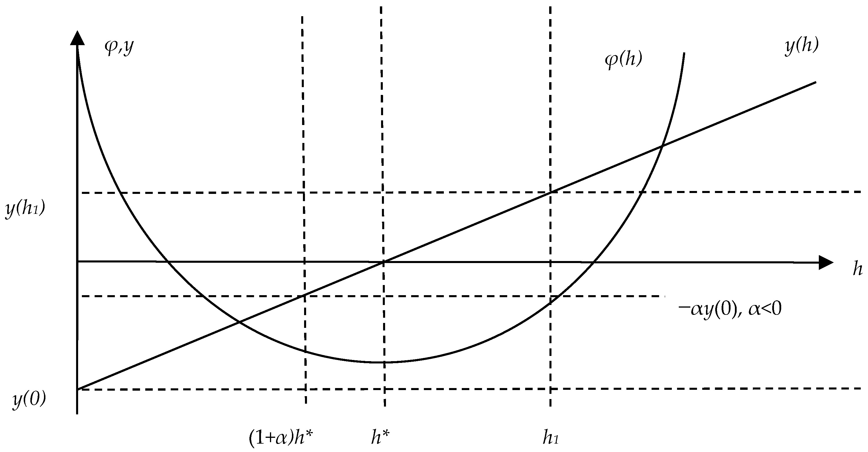
  • The step is too large if there is an obtuse angle between adjacent gradients, that is, ( g k , g k + 1 ) 0 . Therefore, the step should be reduced.
  • If there is an acute angle between adjacent gradients, that is, ( g k , g k + 1 ) > 0 , then the step is too small, and it should be increased.
Another adaptation idea is to replace complete relaxation with some degree of incomplete relaxation or over-relaxation. Another possibility for organizing the step adaptation algorithm is to randomize the strategies of incomplete relaxation and over-relaxation.
Each of the listed strategies determines only the moment of decreasing or increasing the step. Another important question is how and how much to increase or decrease the step at the iteration. Each of the noted strategies should be provided with quantitative values of step updating. In this paper, we use some constant coefficients of step decrease and increase, as well as estimates for the current optimal step in order to use them to calculate the step-adjusting coefficients. The article describes the noted step adaptation strategies and formulates adaptation algorithms. In the next section, these ideas will be formulated in the form of algorithms.

3. Algorithms for Step Adaptation in the Gradient Method

The simplest algorithm for adapting the step of the gradient method is based on the idea of adjusting the orthogonality of successive gradients. If an angle between adjacent gradients is obtuse, ( g k , g k + 1 ) 0 , then the step should be reduced. In the case of an acute angle between adjacent gradients, ( g k , g k + 1 ) > 0 , the step should be increased. The following Algorithm 1 works on this basis.
Algorithm 1 (A1(q))
1. Set q > 1, the search step h0 > 0, the initial point x0.
2. For k = 0,1,2,… do
   2.1 Search for new approximation x k + 1 = x k h k s k , s k = g k / g k .
   2.2 If  ( s k , g k + 1 ) > 0
      then  z k = q
         else  z k = 1 / q .
   2.3 Compute the new search step h k + 1 = z k h k
Condition (8) ( s k , g k + 1 ) = 0 ensures complete relaxation. Here and below, s k = g k / g k . We will consider algorithms with incomplete relaxation and over-relaxation. Denote by y ( h ) = ( f ( x k h s k ) , s k ) a derivative of the function ϕ ( h ) = f ( x k h s k ) with respect to h. If the function is quadratic, then y(h) is a linear function of h. Figure 1 shows this situation.
Assuming the function ϕ(h) is quadratic, based on two observations y(0) and y(h1), we compose a linear representation:
y ( h ) = y ( 0 ) + h y ( h 1 ) y ( 0 ) h 1 .
Denote the step providing (8) by h*. Condition (8) for (9) has the form:
y ( h ) = y ( 0 ) + h y ( h 1 ) y ( 0 ) h 1 = 0 .
Solving (10), we find
h = h 1 y ( 0 ) y ( 0 ) y ( h 1 ) .
In (11), the discrepancy (error) between the current step h1 and the optimal step h* is explicitly given. The error coefficient at the current step can reach large values. Taking into account that the function being minimized is not quadratic, the error coefficient y ( 0 ) / ( y 0 y h 1 ) in (11) can be used to change the step. This enables us to determine the shift of the current step h1 towards the predicted h* using some degree of their convergence, for example,
h + = h 1 y ( 0 ) y ( 0 ) y ( h 1 ) .
In the future, we will use Equation (12) in the adaptation algorithms. To avoid errors associated with noise when calculating y(h), we impose a restriction on the radical expression in (12):
y ( 0 ) y ( 0 ) y ( h 1 ) q , q > 1 .
Considering that the numerator and denominator of the last expression are negative, we may rewrite (13), making them positive: y 0 / y 0 y h 1 q ,   q > 1 . To avoid division errors, the inequality can be written in the following form:
y 0 q y 0 y h 1 ,       q > 1 .
Using (14), we obtain the setting for the step
h + = z × h 1 ,
where
z = q i f   y ( 0 ) > q y ( 0 ) y ( h 1 ) , y ( 0 ) y ( 0 ) y ( h 1 ) o t h e r w i s e .
We use the step tuning (15), (16) in the adaptation Algorithm 2.
Algorithm 2 (A2(q))
1. Set q > 1, the search step h0 > 0, the initial point x0.
2. For k = 0,1,2,… do
   2.1 Search for new approximation x k + 1 = x k h k s k , s k = g k / g k .
   2.2 If  ( s k , g k ) > q ( s k , g k ) ( s k , g k + 1 )
      then  z k = q
         else  z k = ( s k , g k ) ( s k , g k ) ( s k , g k + 1 ) .
   2.3 Compute the new search step
h k + 1 = z k h k

4. Algorithms for the Step Adaptation of the Gradient Method with Incomplete Relaxation, Super Relaxation and Mixed Relaxation

In the previous section, the step was adjusted based on a model h*. In this section, we will choose a model
h = ( 1 + α ) h , α > 1 .
To organize an algorithm of Algorithm 1 type, we need a bound on the scalar product ( s k , g k + 1 ) to decide whether to increase or decrease the current step.
Assuming the function is quadratic, we use model (15) to calculate the boundary
y ( ( 1 + α ) h ) = y ( 0 ) + ( 1 + α ) h y ( h 1 ) y ( 0 ) h 1 = y ( 0 ) + ( 1 + α ) h 1 y ( 0 ) y ( 0 ) y ( h 1 ) y ( h 1 ) y ( 0 ) h 1 = y ( 0 ) ( 1 + α ) y ( 0 ) = α y ( 0 ) .
Exceeding the boundary y ( h ) > α y ( 0 ) means that the step h is too small. The case y ( h ) α y ( 0 ) means that the step is too large (in Figure 1, this boundary is shown by a dotted line for a negative value of α).
Based on (19) and the last remark, we formulate Algorithm 3 with a fixed adaptation step.
Algorithm 3 (A3(q, α))
1. Set q > 1, the search step h0 > 0, the initial point x0, parameter α > −1.
2. For k = 0,1,2,… do
   2.1 Search for new approximation x k + 1 = x k h k s k , s k = g k / g k .
   2.2 If  ( s k , g k + 1 ) > α ( s k , g k )
      then  z k = q
         else  z k = 1 / q .
   2.3 Compute the new search step h k + 1 = z k h k .
In Step 2.2, the value α ( s k , g k ) acts as a boundary for the step adaptation parameter ( s k , g k ) .
Next, we will consider adaptation based on the predicted step value using a quadratic model of the function. From (12), we obtain
h α = ( 1 + α ) h = h 1 ( 1 + α ) y ( 0 ) y ( 0 ) y ( h 1 ) .
As an adjusted step, we will take the following:
h + = h 1 ( 1 + α ) y ( 0 ) y ( 0 ) y ( h 1 ) .
Instead of expression (21), we can use dependencies reflecting the tendency h + h α .
Further, in the adaptation algorithms, we will use Equation (21). To avoid errors associated with noise when calculating y(h), we impose a restriction on the radical expression in (12):
( 1 + α ) y ( 0 ) y ( 0 ) y ( h 1 ) q , q > 1 .
Considering that the numerator and denominator of the last expression are negative, we may rewrite (22), making them both positive: ( 1 + α y 0 ) / y 0 y h 1 q ,   q > 1 . To avoid division errors, the inequality can be written in the following form:
( 1 + α ) y ( 0 ) q y ( 0 ) y ( h 1 ) ,   q > 1 .
Using (23), we obtain step adjusting:
h + = z h 1 ,
where
z = q i f   ( 1 + α ) y ( 0 ) > q y ( 0 ) y ( h 1 ) , ( 1 + α ) y ( 0 ) y ( 0 ) y ( h 1 ) o t h e r w i s e .
Let us formulate the algorithm of the gradient method with step adaptation taking into account the predicted value and type of relaxation (21). We use the step tuning (24), (25) in the adaptation algorithm (Algorithm 4).
Algorithm 4 (A4(q, α))
1. Set q > 1, the search step h0 > 0, the initial point x0, parameter α > −1.
2. For k = 0,1,2,… do
   2.1 Search for new approximation x k + 1 = x k h k s k , s k = g k / g k .
   2.2 If  ( 1 + α ) ( s k , g k ) > q ( s k , g k ) ( s k , g k + 1 )
      then  z k = q
         else  z k = ( 1 + α ) ( s k , g k ) ( s k , g k ) ( s k , g k + 1 ) .
   2.3 Compute the new search step
h k + 1 = z k h k .
We organize mixed step adaptation by randomizing the parameter α
α [ a , b ] ,   a > 1 ,   b > a .
In our numerical experiments, we used uniform distribution on the segment when choosing the parameter α in accordance with (27). The algorithm of the gradient method with step adaptation with randomized predicted value and type of relaxation (21) is presented below. We use the step tuning (24), (25) in the adaptation algorithm (Algorithm 5).
Algorithm 5 (A5(q, α[a, b]))
1. Set q > 1, the search step h0 > 0, the initial point x0, parameters of the segment [a, b] a > −1, b > a.
2. For k = 0,1,2,… do
   2.1 Search for new approximation x k + 1 = x k h k s k , s k = g k / g k .
   2.2 Set α ∈ [a, b].
   2.3 If  ( 1 + α ) ( s k , g k ) > q ( s k , g k ) ( s k , g k + 1 )
      then  z k = q
         else  z k = ( 1 + α ) ( s k , g k ) ( s k , g k ) ( s k , g k + 1 ) .
   2.4 Compute the new search step
h k + 1 = z k h k .
In the next section, the efficiency of the proposed step-adaptive gradient method algorithms will be investigated on test functions.

5. Convergence Analysis

Let us study the change in the convergence rate when applying to a gradient a relative interference uniformly distributed on a ball of radius
R ( x ) = Δ f ( x ) .
Approximate estimates of costs for a given Δ are based on a comparison of estimates for Δ = 0. In methods for solving systems of equations, any estimates are based on the use of the boundaries of the matrix eigenvalues. In this case, if a gradient method with a constant step is used, then its step is determined based on the boundaries of the eigenvalues spectrum.
We do not have the boundaries of the matrices of second derivatives for the functions being minimized; however, these matrices also vary significantly depending on the current point. For an approximate estimate of the dependence of costs on Δ, we obtain a relation for the simplest quadratic function and calculate the increase in these costs compared to Δ = 0. Considering that the estimates of the convergence rate on quadratic functions of the gradient method with an optimal step coincide with the estimates of the convergence rate for the steepest descent method, we will use the results for the steepest descent method when correlating the results with noise.
Let us estimate the convergence rate of the gradient method with a constant step in the presence of noise. Consider a one-dimensional function whose gradient is calculated with noise
f ( x ) = x 2 / 2 , f ( x ) = g ( x ) = x + Δ | x | η , η [ 0 , 1 ] ,
where η is a random number. To minimize it, we use a gradient method with a constant step
x + = x h g = x h ( x + Δ | x | η ) = x ( 1 h ) h Δ | x | η .
Find the expectation
M ( x + ) 2 = M ( x ( 1 h ) h Δ | x | η ) 2 = x 2 ( 1 h ) 2 + h 2 Δ 2 x 2 U = x 2 ( ( 1 h ) 2 + h 2 Δ 2 U ) = x 2 ( 1 2 h + h 2 ( 1 + Δ 2 U ) ) ,
where U = M(η2).
For a uniform distribution η on a unit ball with n = 2, it can be calculated as follows:
U = 0 1 r 2 2 π r d r / 0 1 2 π r d r = 1 / 2 .
For a uniform distribution η on a unit ball with large n values, U ≈ 1.
Expression (32), according to (30), determines the change in the function at the iteration. Let us find the optimal step based on (32)
( 1 2 h + h 2 ( 1 + Δ 2 U ) ) = 2 + 2 h ( 1 + Δ 2 U ) = 0 .
Therefore, h* = 1/(1 + Δ2U).
When minimizing multidimensional functions, the optimal step would be significantly smaller due to the spectrum boundaries of the second derivatives matrix. Therefore, we use the step
h = q h = q / ( 1 + Δ 2 U ) , q < 1 .
for the evaluation of the indicator 1 − 2h + h2(1 + Δ2U) from (32). Then,
Q ( Δ ) = 1 2 h + h 2 ( 1 + Δ 2 U ) = 1 2 q / ( 1 + Δ 2 U ) + q 2 ( 1 + Δ 2 U ) / ( 1 + Δ 2 U ) 2 = 1 2 q / ( 1 + Δ 2 U ) + q 2 / ( 1 + Δ 2 U ) 1 q / ( 1 + Δ 2 U ) exp ( q / ( 1 + Δ 2 U ) ) .
Therefore,
Q ( 0 ) = Q ( Δ ) 1 + Δ 2 U .
Denote by N(Δ) the number of iterations of the method to achieve a given accuracy for the function. Then, according to (37), the cost ratio will be as follows:
N ( Δ ) = ( 1 + Δ 2 U ) N ( 0 ) .
We use the dependence on the magnitude of the noise (38) to estimate the number of iterations in our problems. Since the estimates for the steepest descent method and the gradient method with the choice of the optimal step for minimizing quadratic functions coincide, we will use the number of iterations of the steepest descent method as N(0).

6. Numerical Experiment

Our experiments were performed on smooth test functions, where the usual steepest descent method converges with the geometric progression rate. The minimum of test functions is uniquely defined. Test functions include functions with curvilinear ravines and functions that differ significantly in properties from quadratic ones. The tests take into account nonlinearities, non-quadraticity and the curvature of ravines with different degrees of problem determination. The calculations are carried out for a number of dimensions.
The local behavior of algorithms in a local region of some nonlinear function where there is a bounded matrix of second derivatives is reflected in tests on a quadratic function at different degrees of conditionality. These data can be extrapolated to non-quadratic functions with an existing matrix of second derivatives, where the number of iterations required is several times greater.
The objectives of the numerical experiment are as follows:
  • Evaluate the efficiency of the proposed algorithms and compare their efficiency with the efficiency of the steepest descent method under conditions without interference.
  • Determine the effects of convergence acceleration in the proposed methods and identify modifications that have accelerated convergence.
  • Study the effect on the convergence rate when applying a gradient of relative interference uniformly distributed on a ball of radius R ( x ) = Δ f ( x ) .
  • Make estimates of the iteration costs given (29).
Denote the steepest descent method by GR. Among the methods presented above, the following algorithms were used: Algorithm 1 (A1(q)), Algorithm 2 (A2(q)), Algorithm 4 (A4(q, α)), Algorithm 5 (A5(q, α[a, b])).
In all methods, the function and gradient were calculated simultaneously. In step-adaptive algorithms, function calculations are not required. The stopping criterion was f ( x k ) f ε .
Table A1, Table A2, Table A3, Table A4, Table A5, Table A6, Table A7, Table A8, Table A9, Table A10, Table A11, Table A12, Table A13, Table A14, Table A15, Table A16, Table A17, Table A18, Table A19, Table A20, Table A21, Table A22 and Table A23 show the number of iterations (the number of gradient calculations) for the methods with step adaptation. For the gradient method (GR), the number of iterations and the number of calculations of the function and gradient used to form the descent direction and one-dimensional minimization are given. We will compare the efficiency of the methods only by the number of iterations. The values of x0 and ε are given in the description of the corresponding function.

6.1. Rosenbrock Function

The Rosenbrock function has the form:
f R ( x ) = 100 ( x 2 x 1 2 ) 2 + ( x 1 1 ) 2
Its minimum point is x* = (1, 1)T. Two points were selected as starting points: x1T = (0, 0), x2T = (−1.2, 1). The stopping criterion was f ( x k ) f ε = 10 10 .
In Table A1 and Table A2, the number of iterations of the algorithms A4(q, α)), A5(q, α[a, b]) and GR method required to achieve a given accuracy for different α values is presented. One-dimensional search in the steepest descent method was performed based on cubic interpolation using function and gradient information.
Table A1 and Table A2 and Figure 2 show calculations for large values of q, where the convergence rate turned out to be higher. But, as we will see below, for functions with a lower degree of conditionality, the costs will be just as high with such parameters, and for small q, these costs will be significantly lower. This problem of equal efficiency for different degrees of conditionality is solved by randomization of the A5 algorithm. The application of this algorithm is equally effective at different levels of conditionality. Also, this algorithm allows obtaining more effective results at a low interference level.
In Table A3 and Figure 3, the results of minimization with interference are presented. The first column of the table indicates the interference parameter Δ imposed in accordance with (29). It is assumed that the interference is uniformly distributed in the sphere. For some functions, the interference is distributed on the surface of the sphere, which will be specifically discussed. Empty cells here and below mean that the algorithm does not converge as the noise level increases.
On this function, the algorithms A1(q), A2(q) are approximately the same and can withstand significant interference. Here is an example where the radius of the interference ball is 8 times greater than the gradient norm. In the case of interference, the algorithm A5(q, α[a, b]) turned out to be effective, but only for small interference values.

6.2. Quadratic Function

The following quadratic function is tested:
f Q ( x , [ a max ] ) = 1 2 i = 1 n a i x i 2 , a i = a max i 1 n 1 .
The eigenvalues ai of this function have the boundaries λmin = 1 and λmax = amax. The starting point was x0T = (100, 100, …, 100). The stopping criterion was f ( x k ) f ε = 10 10 .
Table A4, Table A5 and Table A6 and Figure 4 show the results of function minimization for different degrees of conditionality.
Depending on the conditionality of the problem, the algorithm A4(q = ∞, α) has good results for different values of α. The algorithm A5(q = ∞, α[a, b]) has equally good results, surpassing the results of the steepest descent method.
Conclusions can be drawn regarding the convergence rate of algorithms:
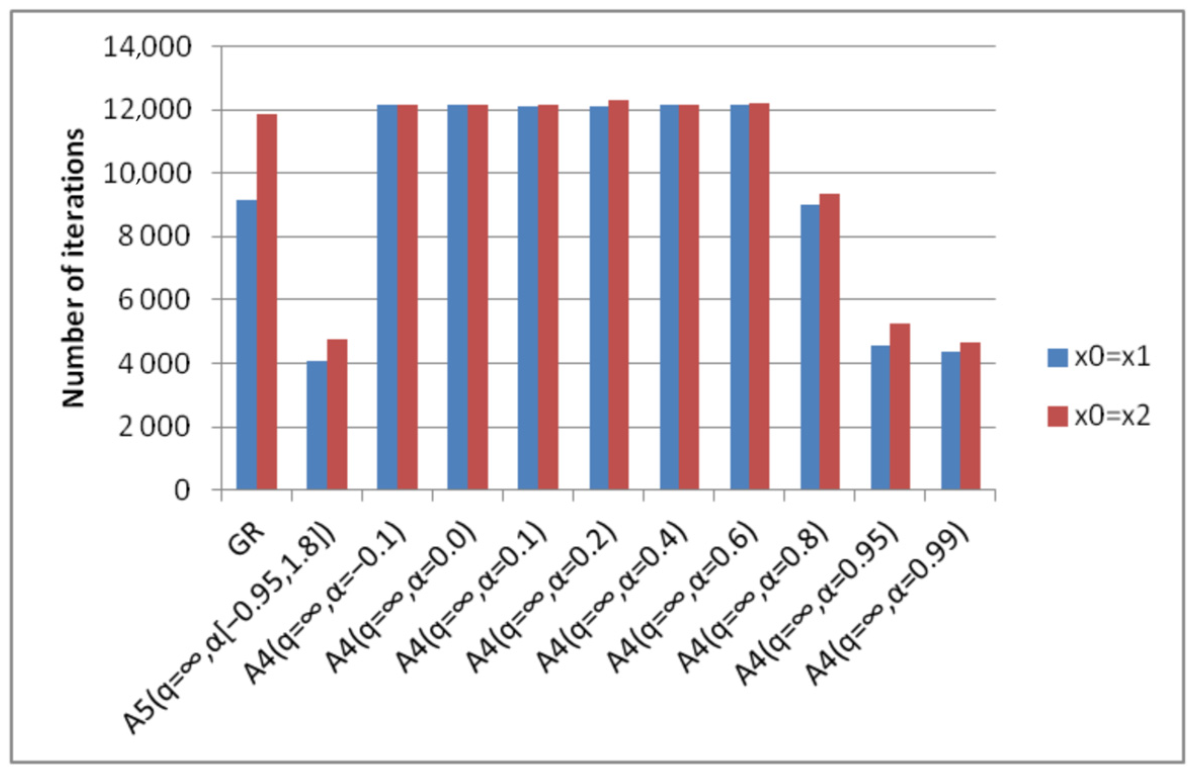
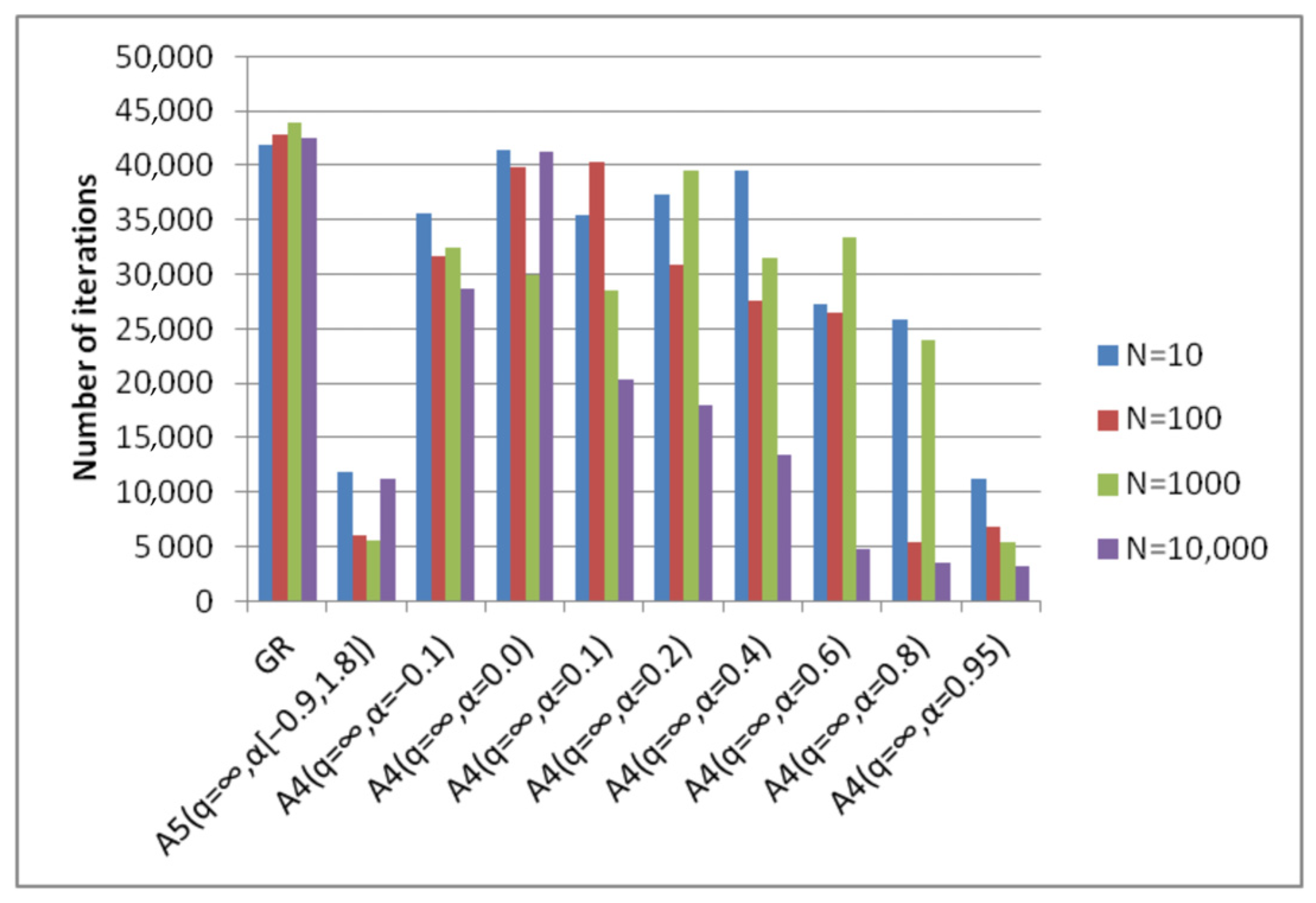
  • Algorithm A4(q = ∞, α) achieves good results with different parameters α for different degrees of conditionality. This parameter can only be determined experimentally.
  • Algorithm A5(q = ∞, α[a, b]) achieves good results with fixed parameters of the algorithm for different degrees of conditionality. From this point of view, it can be considered universal.
  • The best versions of algorithm A4(q = ∞, α) and algorithm A5(q = ∞, α[a, b]) are less expensive in terms of the number of iterations compared to the gradient method.
Table A7 and Figure 5 shows the results of minimizing a quadratic function under gradient interference for dimension N = 1000.
On this function, the algorithms A1(q), A2(q) are approximately the same and can withstand significant interference. Here is an example where the radius of the interference uniformly distributed in the ball is 8 times greater than the gradient norm. In the case of interference, the algorithm A5(q, α[a, b]) turned out to be not so effective even for small values of the error level.

6.3. Functions with Ellipsoidal Ravine

The following function has a multidimensional ellipsoidal ravine. Minimization occurs when moving along a curvilinear ravine to the minimum point.
f E E L ( x , [ a max , b max ] ) = ( 1 x 1 ) 2 + a max 1 i = 1 n x i 2 / b i 2 , b i = b max i 1 n 1
The starting points were x1 = (−1, 0.1, …, 0.1), x2 = (−1, 2, 3, …, n). The stopping criterion was f ( x k ) f ε = 10 4 .
Table A8, Table A9 and Table A10 and Figure 6 and Figure 7 demonstrate the results of function fEEL minimization.
Algorithm A4(q = ∞, α) has good results for different values of α for different initial points and dimensions of the problem. That is, a preliminary experiment is required to select the optimal parameters. Algorithm A5(q = ∞, α[a, b]) has good results regardless of changes in the dimension and degree of conditionality of the problem. Its results in terms of the number of iterations exceed the results of the steepest descent method.
On this function, the algorithms A1(q), A2(q) are approximately the same and withstand significant interference. Here, the interference is uniformly distributed in the ball, the radius of which is 8 times greater than the gradient norm. In the case of interference, the algorithm A5(q, α[a, b]) shows good results only at a low level of interference.
The convergence rate of the algorithms A1(q), A2(q) depends little on the interference. This is explained by the presence of a ravine, where interference creates the possibility of moving not to the bottom of the ravine, but along it.
In order to make the dependence of the iterations number on the magnitude of interference noticeable, in the next test, we reduced the dimension, and the interference on the gradient was made uniformly distributed on the surface of the ball for different values of the gradient interference parameter (29). Table A11, Table A12 and Table A13 and Figure 8 and Figure 9 demonstrate the results.
On this function, the algorithms A1(q), A2(q) are approximately equal in efficiency and can withstand significant interference. Here, the interference is uniformly distributed over the surface of the sphere. In the case of interference, the algorithm A5(q, α[a, b]) shows good results at a low level of interference. Here, the dependence of the convergence rate of the algorithms A1(q), A2(q) on the magnitude of interference appears more clearly.
In Figure 9, the degree of degeneracy of the ravine has increased compared to the previous example. Algorithm A4(q = ∞, α) has good results for α = 0.95. Algorithm A5(q = ∞, α[a, b]) has good results, significantly exceeding the results of the steepest descent method, which confirms its universality.
In Figure 10, algorithms A1(q), A2(q) are approximately equal in efficiency at the interference level Δ ≤ 5. At higher values, algorithm A2(q) shows better results. Both algorithms withstand significant interference. Here, the interference is uniformly distributed on the surface of the sphere. In the case of interference, algorithm A5(q, α[a, b]) shows good results at a low interference level.
The next function also has a multi-dimensional ellipsoidal ravine.
f E E L X ( x , [ a max ] ) = ( 1 x 1 ) 2 + a max 1 i = 1 n x i 2 b i 2 + 1 2 i = 1 n x i 2 b i , b i = b max i 1 n 1 ,   b max = 10 .
The starting points were x1 = (−1, 0.1, …, 0.1), x2 = (−1, 2, 3, …, n). The stopping criterion was f ( x k ) f ε = 10 10 . Due to the additional term in fEELX, the minimum point ceases to be singular. This allows the gradient method to find the minimum of the function at higher ravine coefficients amax with higher accuracy compared to the function fEEL. Table A14, Table A15 and Table A16 and Figure 11 and Figure 12 show the results of function fEELX minimizing.
On this function, the degree of the ravine degeneracy has increased compared to the previous function fEEL. Algorithm A4(q = ∞, α) has good results for α = 0.95. Algorithm A5(q = ∞, α[a, b]) has good results, significantly exceeding the results of the steepest descent method, which, together with the results of minimization of the previous functions, confirms its universality.
On this function, the A1(q) algorithm slightly outperforms the A2(q) algorithm. This is due to the decrease in the step tuning value in A1(q = 1.01) from the previous q = 1.1. Both algorithms withstand significant interference. Unlike the previous results, here, the interference is uniformly distributed over the sphere. In the case of interference, the A5(q, α[a, b]) algorithm shows good results at a low interference level. As the interference level increases, the A5(q, α[a, b]) algorithm ceases to converge.
The following function was used to analyze the effect of noise on the gradient components.
f Q ^ 2 ( x , [ a max ] ) = i = 1 n a i x i 2 2 , a i = a max i 1 n 1 , x 0 = ( 1 , 1 , , 1 ) .
The matrix of second derivatives of this function tends to zero as it approaches the minimum. The stopping criterion was f ( x k ) f ε = 10 10 . Table A17, Table A18, Table A19 and Table A20 and Figure 13 and Figure 14 show the results of function fQ^2 minimization for different degrees of elongation of the level surfaces.
Depending on the elongation of the function level surfaces, the algorithm A4(q = ∞, α) has good results for the same values of α = 0.95. The algorithm A5(q = ∞, α[a, b]) has equally good results, surpassing the results of the steepest descent method.
The following conclusions can be drawn regarding the convergence rate of the algorithms:
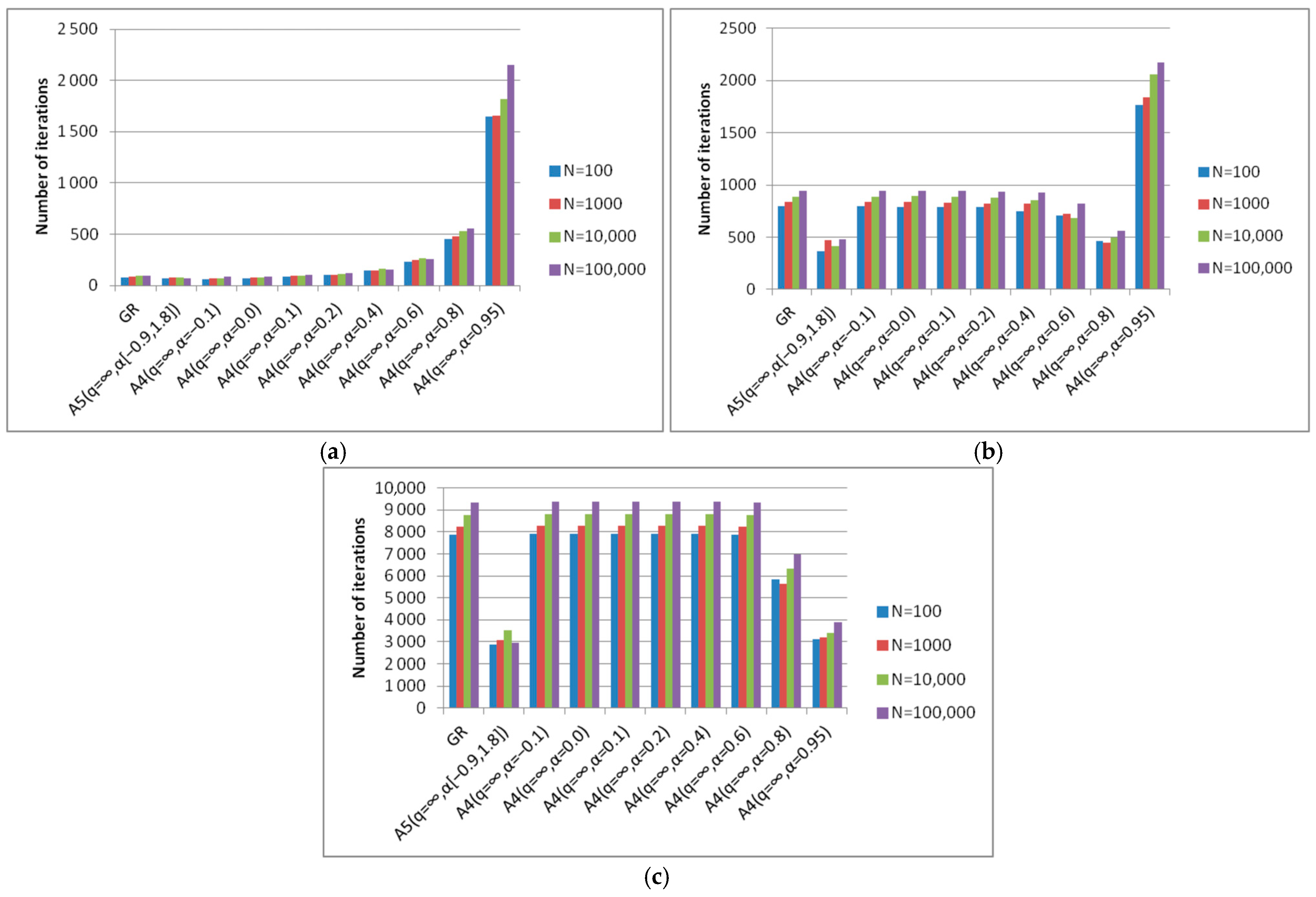
  • Algorithm A4(q = ∞, α) achieves good results at α = 0.95 for various degrees of elongation of the level surfaces. This parameter can only be determined experimentally.
  • Algorithm A5(q = ∞, α[a, b]) achieves good results with fixed algorithm parameters for various degrees of elongation of the level surfaces. From this point of view, it confirms its universality.
  • The best versions of algorithm A4(q = ∞, α) and algorithm A5(q = ∞, α[a, b]) are less expensive in terms of the number of iterations compared to the steepest descent method.
On this function, the algorithms A1(q), A2(q) are approximately equivalent in efficiency. In the case of interference, the algorithm A5(q, α[a, b]) turned out to be more efficient only for small values of the noise level. In the case of a strongly elongated curvilinear ravine (at amax = 10,000), algorithms A1(q), A2(q) with their given parameters failed to obtain a solution at interference level Δ > 6. As experience in testing the algorithms A1(q), A2(q) shows, reducing the step boundary q allows to obtain a solution for large values of interference. At the same time, with small interference, there is some slowdown in the convergence rate.
The next for testing was the Raydan1 function. It is biased to obtain a new function with a zero minimum value:
f R ( x , [ a max ] ) = i = 1 n a i 10 ( exp ( x i ) x i 1 ) , a i = a max i 1 n 1 , x 0 = ( 2 , 2 , , 2 )
The stopping criterion was f ( x k ) f ε = 10 10 . In this function, the banks of the ravine differ significantly in steepness. The behavior of the gradient method with step adaptation under such conditions is of interest. Table A21, Table A22 and Table A23 and Figure 15 and Figure 16 demonstrate the results of function fR minimization.
Figure 15 shows the results of function minimization for different degrees of elongation of the level surfaces. Depending on the elongation of the function level surfaces, the A4(q = ∞, α) algorithm has good results for different values of α. The A5(q = ∞, α[a, b]) algorithm has equally good results, surpassing the results of the steepest descent method.
On this function, algorithms A1(q), A2(q) are approximately equivalent in efficiency. In the case of interference, algorithm A5(q, α[a, b]) turned out to be not so efficient even for small values of the error level.

7. Discussion

To illustrate the convergence of the abovementioned algorithms, we consider the logarithm of the minimization error f ( x k ) f against iterations for the quadratic function fQ (Figure 17).
As can be seen, a linear convergence rate takes place. Methods GR and A4(q = ∞, α) are almost equivalent, although the GR method uses a one-dimensional search. Moreover, method A5(q, α[a, b]) has a higher linear convergence rate.
In real minimization problems, the costs of methods are proportional to the dimension and are small compared to the time to calculate the function and gradient. Since the main costs are incurred in calculating the function and gradient, the steepest descent method requires at least calculating the function and gradient. The proposed method calculates only one gradient, which means that compared to the steepest descent method, the time is reduced by more than 2 times.
The iteration runtime for the considered methods is presented in Table 1 and Figure 18. The runtime for the A4(q = ∞, α) and A5(q, α[a, b]) methods is equivalent.
Let us test the theoretical convergence analysis in practice. For the Rosenbrock function, the cost of the number of iterations of the steepest descent method for different initial points is 9150 and 11,865 iterations. For Δ = 3, taking into account (33) and (38), we obtain N(Δ) = (1 + Δ2U)N(0) = (1 + 9/2)N(0) = 5.5N(0). For different initial points, we obtain N(Δ) = 50,325 and N(Δ) = 65,260, while the actual costs are 59,616 and 43,264.
For Δ = 8, we obtain N(Δ) = 33N(0). For different initial points N(Δ) = 30,1950 and N(Δ) = 351,543, the actual costs are 97,469 and 379,943. For the Rosenbrock function, we obtained a good match between the calculated and real data, although the Rosenbrock function is far from a quadratic function.
For a quadratic function, the cost of the number of iterations of the steepest descent method for different function coefficients is 835 and 8239. For Δ = 3 N(Δ) = (1 + Δ2U)N(0) = (1 + 9)N(0) = 10N(0). The theoretical values are N(Δ)= 8350 and N(Δ)= 82,390, while the actual costs are 3440 and 28,925. For Δ = 8, we obtain N(Δ) = 65N(0). The theoretical values are N(Δ)= 54,275 and N(Δ)= 535,535, while the actual costs are 23,166 and 153,001.
For the quadratic function, the actual results were even better than the estimates. At the same time, the actual data are more consistent with the use of the A5(q = ∞, α[a, b]) algorithm as N(0) data.
The question arises as to why in many cases deviation from the step selection of the steepest descent method yields better results. In linear algebra, there is a multi-step optimal process for solving systems of linear equations, the parameters of which are calculated based on the boundaries of the matrix spectrum. But it turns out that this process can be implemented as a gradient method, the steps of which are calculated based on Chebyshev polynomials. The steepest descent method descends into a ravine and moves toward a minimum in small steps. In the case of variability of steps, there is a move away from the ravine, which allows moving toward a minimum with large steps. In our case, in the A5(q = ∞, α[a, b]) algorithm, there is a change in the step, which makes it oscillatory to a certain extent, which facilitates movement with large steps. In the case of interference due to randomness in the direction, the method has large oscillations relative to the ravine, which facilitates faster movement toward the minimum. This is probably why real results for a quadratic function give better results.
Let us summarize the features of the studied algorithms with step adaptation in the gradient method in the cases without interference and with interference.
Without interference:
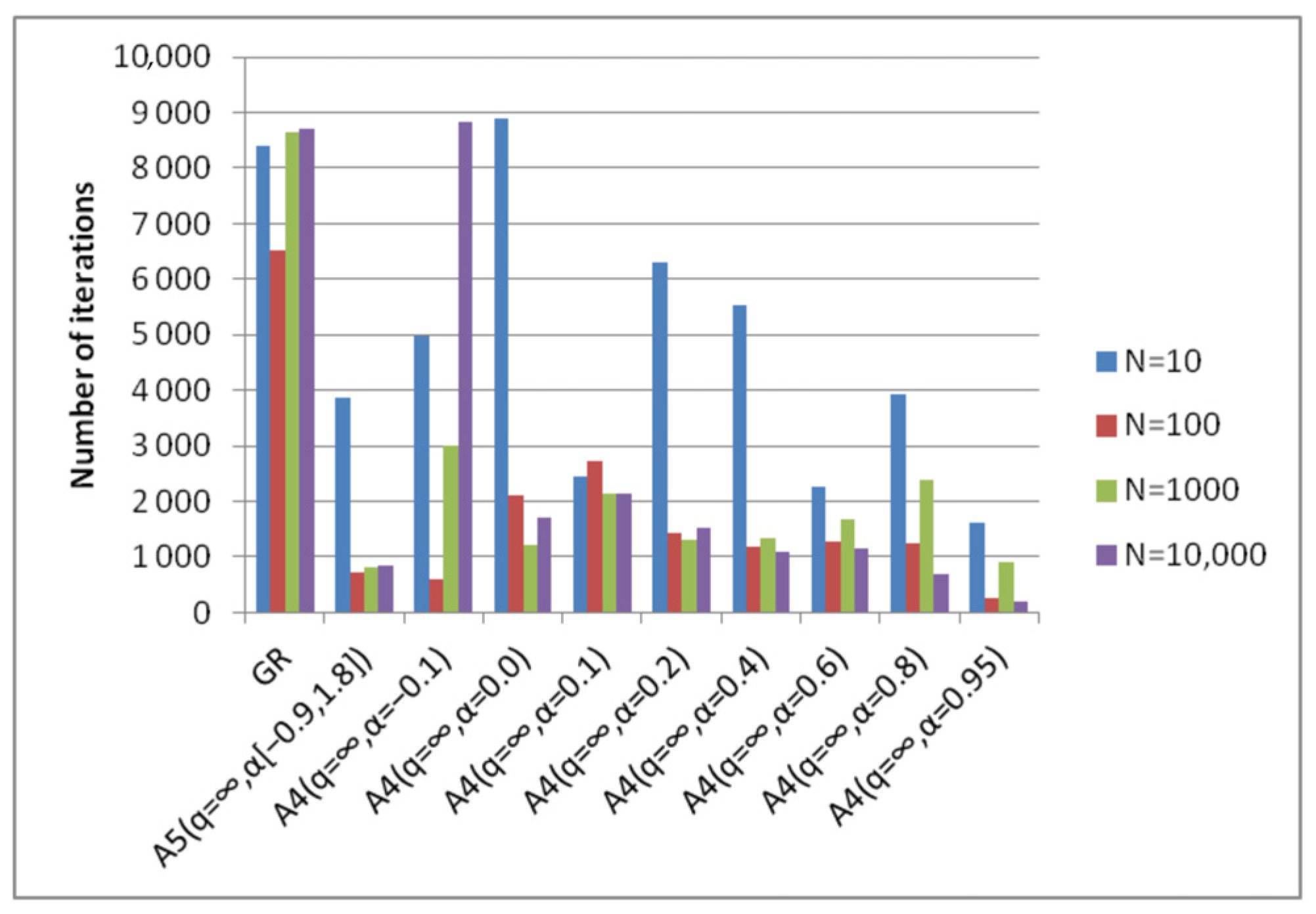
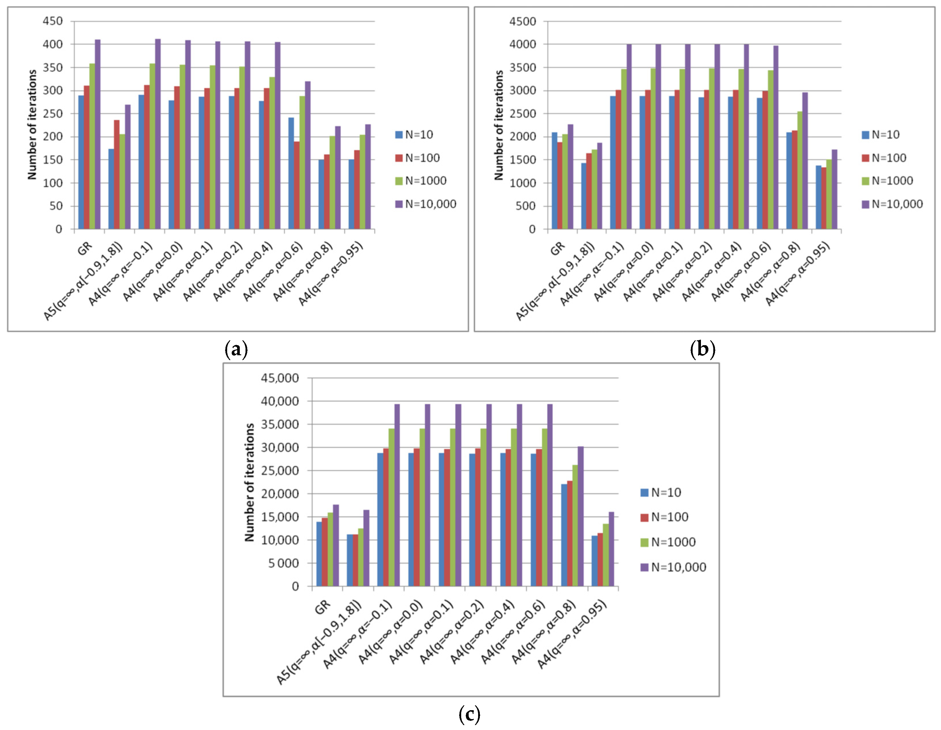
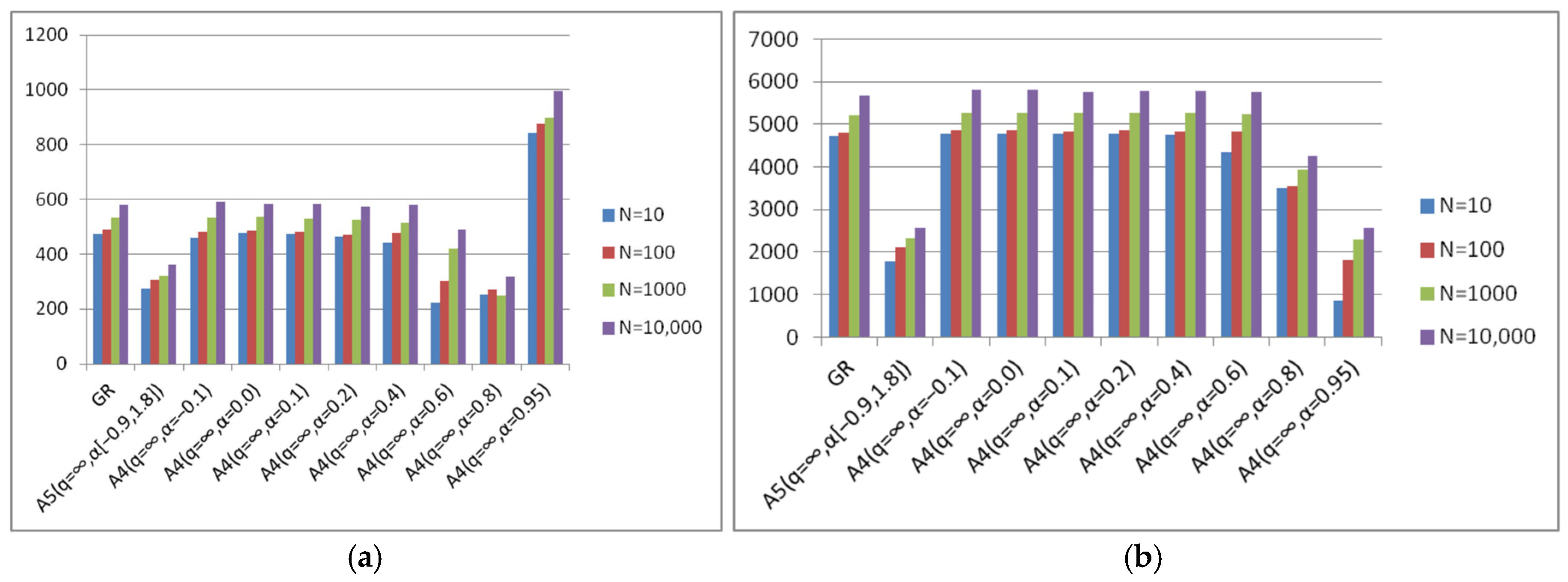
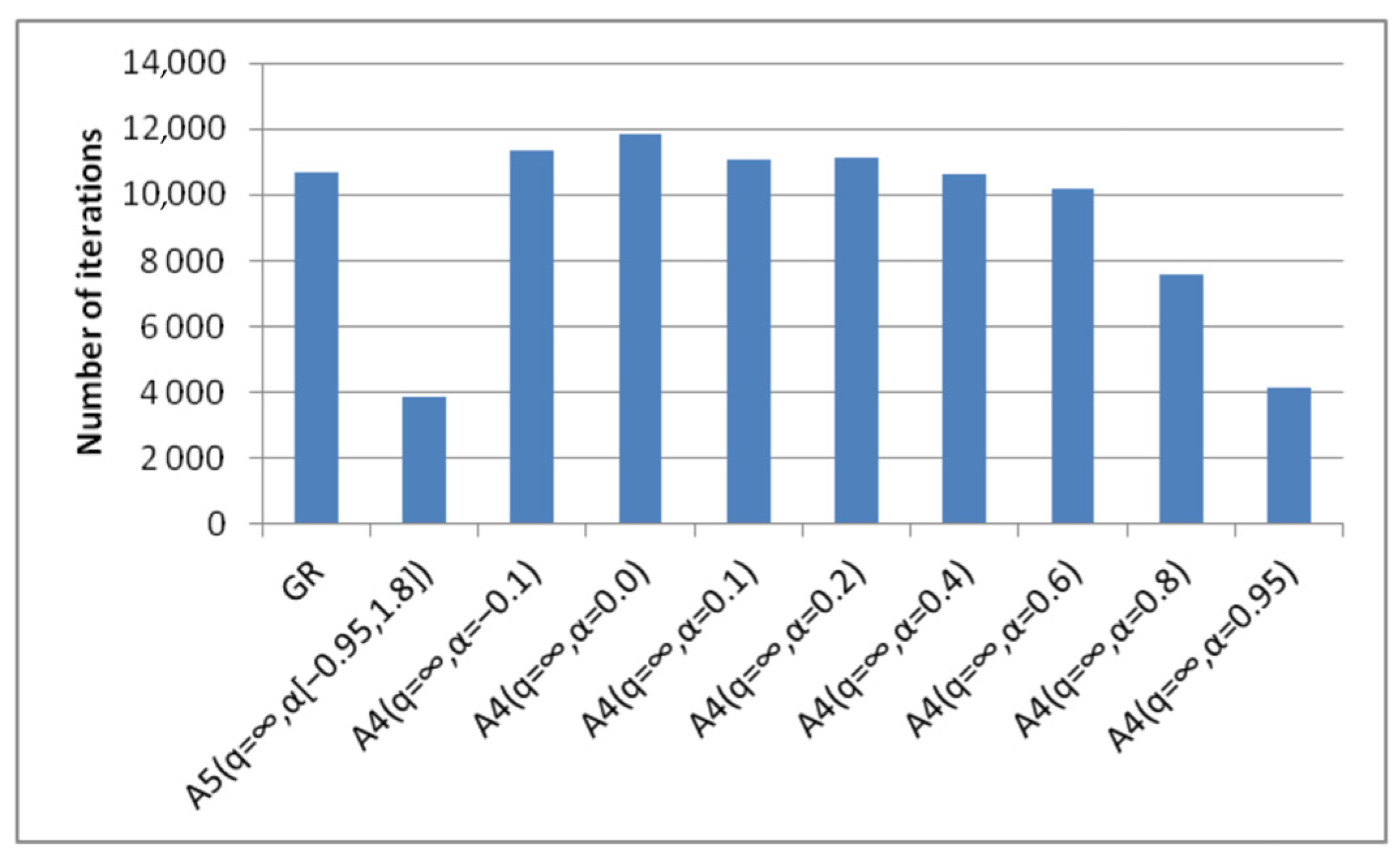
  • Algorithm A4(q = ∞, α) achieves the best (minimal) results with different parameters α, which depend on the degree of conditionality of the problem and the choice of the starting point (Figure 19).
  • The best results of algorithm A4(q = ∞, α) are either comparable or significantly exceed the results of the steepest descent method in the number of iterations.
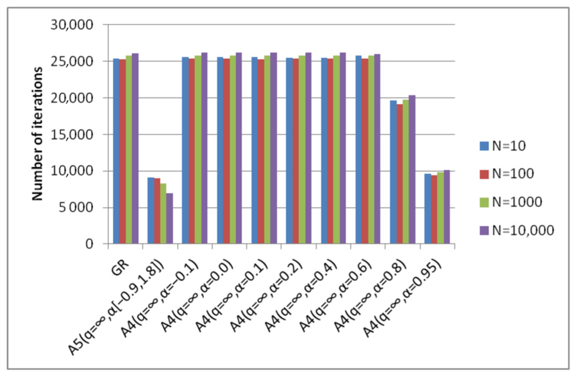
  • The results of algorithm A5(q = ∞, α[a, b]) with fixed parameters correspond to the results of the optimal algorithm A4(q = ∞, α) (Figure 20). This means that there is no need to preliminarily choose the parameters for the A4(q = ∞, α) algorithm. To obtain optimal results one can use the A5(q = ∞, α[a, b]) algorithm, the parameters of which are fixed.
With interference:
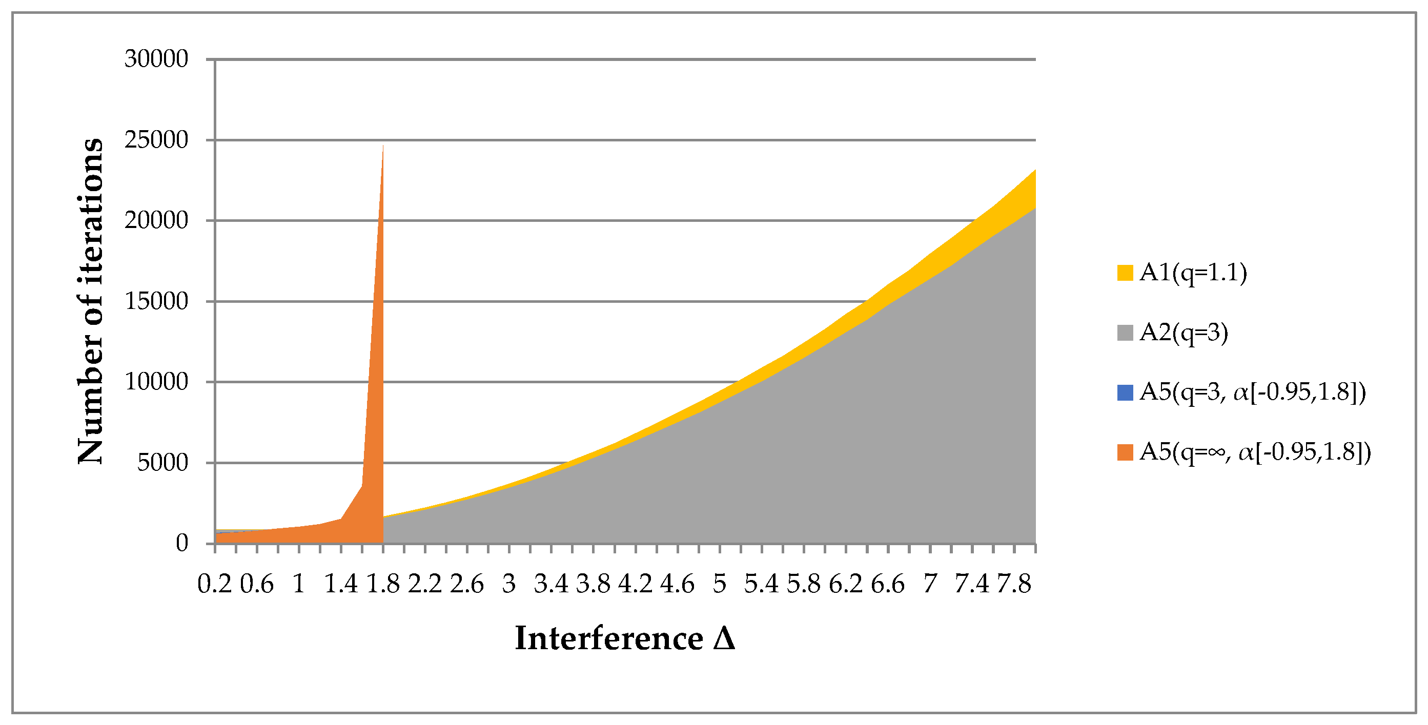
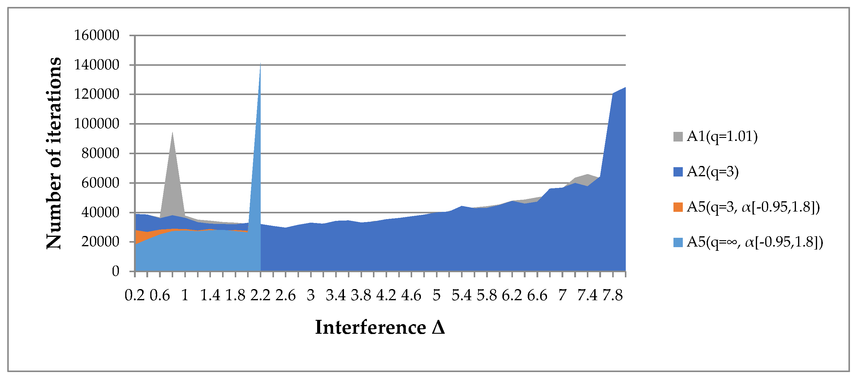
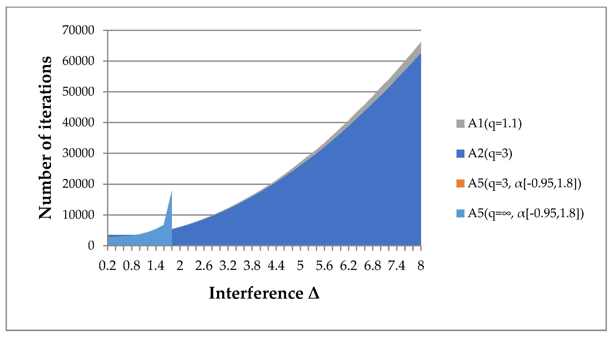
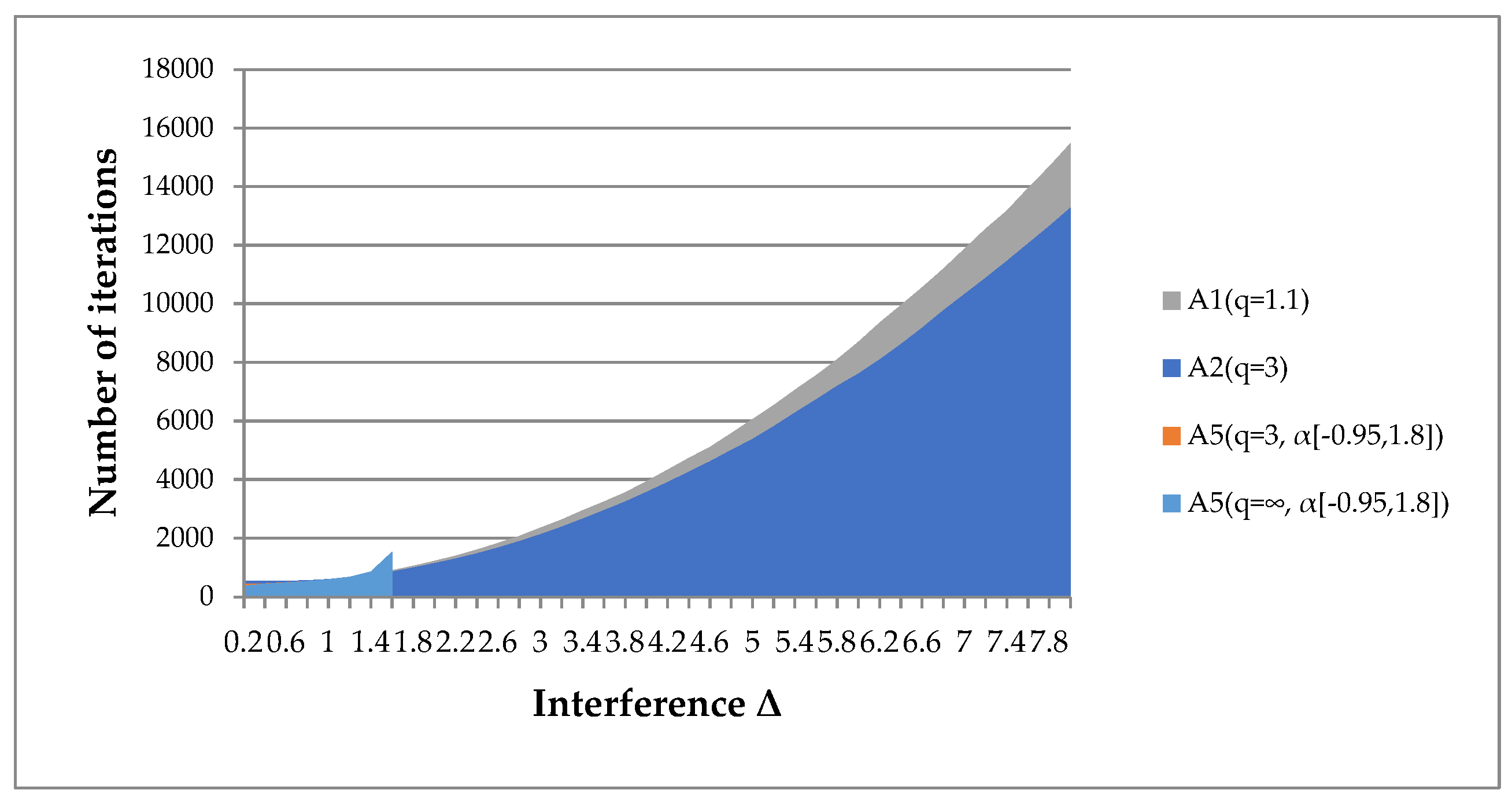
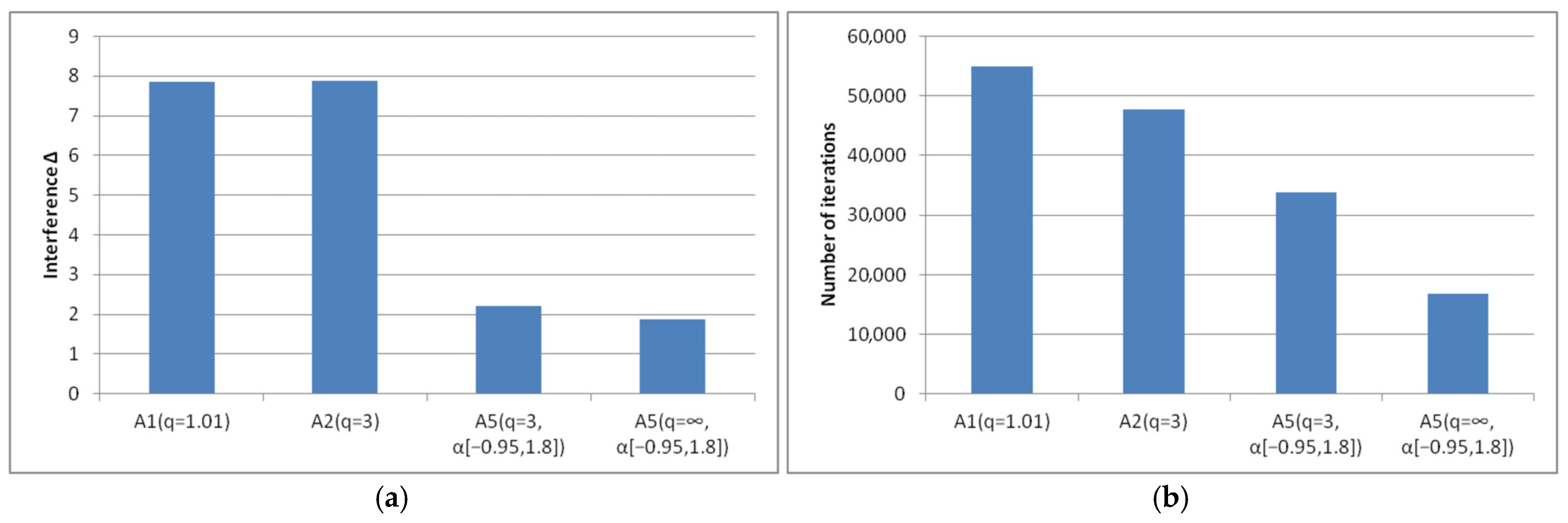
  • Algorithm A5(q, α[a, b]) is applicable only for minor interference. However, its results are not always more significant than the results of algorithms A1(q), A2(q).
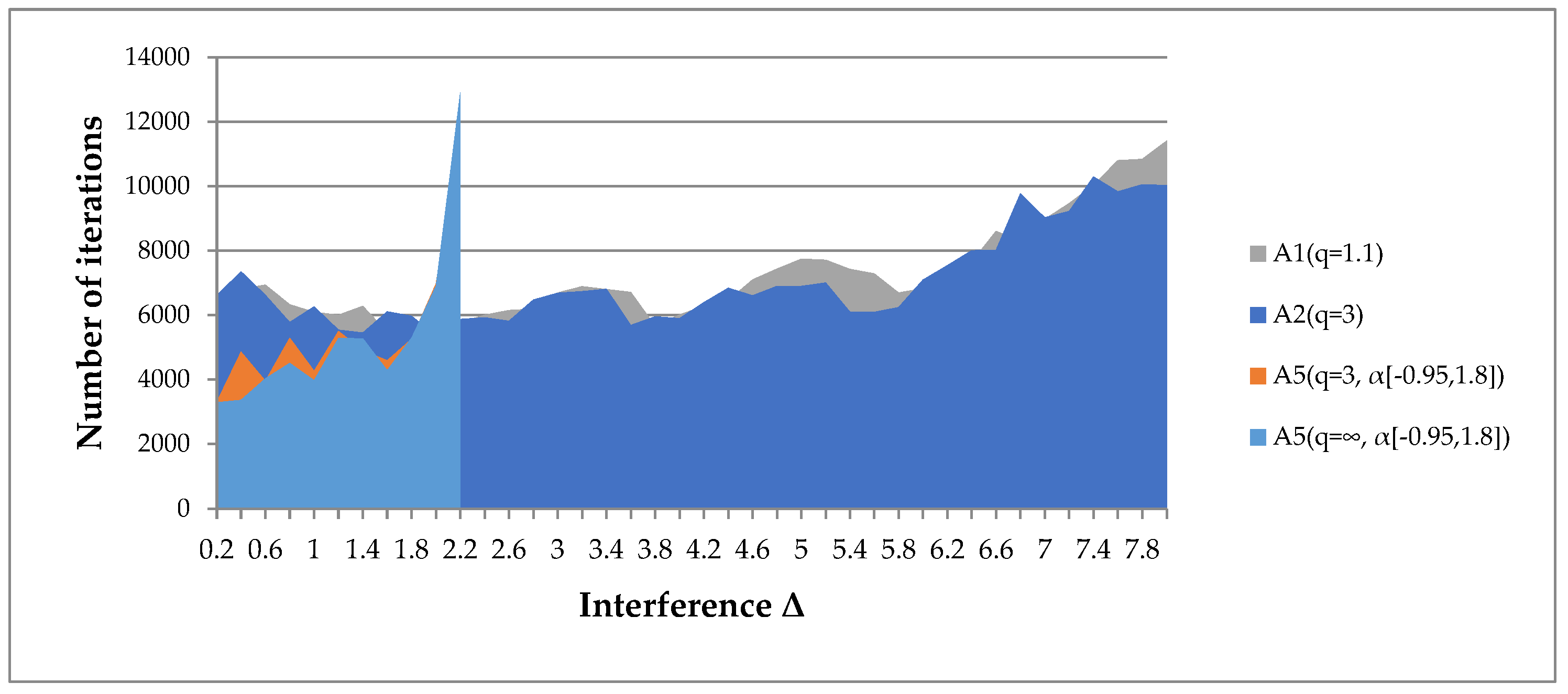
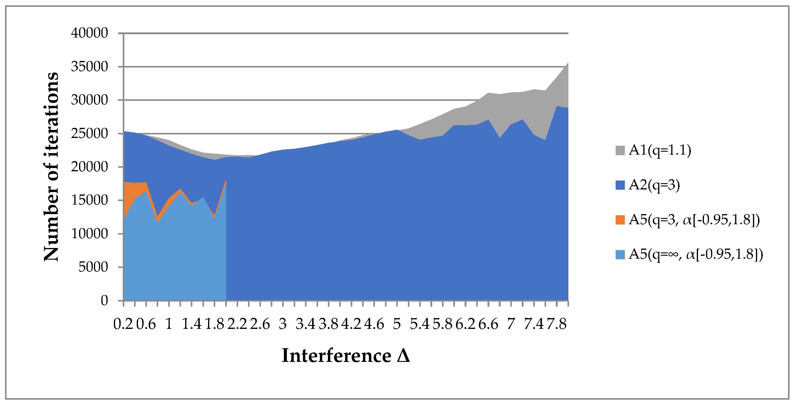
  • Algorithms A1(q), A2(q) are applicable for high interference levels. We have given examples where the radius of the interference uniformly distributed in the sphere exceeds the gradient norm by 8 times (Figure 21a).
  • The convergence of algorithms A1(q), A2(q) depends on the restrictions imposed on the parameter q (Figure 21b). For smaller values of the parameter q, the algorithms are efficient at a higher interference level. However, the convergence rate slows down. For smaller values of the boundary q, results can be obtained even with a 10-fold excess of the interference radius over the gradient norm.

8. Conclusions

The paper solves the problem of constructing step adaptation algorithms for a gradient method based on the principle of the steepest descent method. Expanding the step adjustment principle, its formalization and parameterization led to gradient-type methods with incomplete relaxation or over-relaxation. In such methods, only the function gradient needs to be calculated at the iteration. Optimization of the step adaptation algorithm parameters enables us to obtain methods that significantly exceed the steepest descent method in convergence rate.
We present a universal step adjustment algorithm that does not require selecting optimal parameters, and its convergence rate corresponds to algorithms with optimization of the step adaptation algorithm parameters. The advantage of the proposed method is its operability under interference conditions. Our paper presents examples of solving test problems in which the interference level is in the form of a uniformly distributed vector in a ball whose radius is 8 times greater than the gradient norm.

Author Contributions

Conceptualization, V.K.; methodology, V.K., E.T. and S.G.; software, V.K.; validation, L.K., E.T., I.R. and S.G.; formal analysis, L.K. and S.G.; investigation, V.K.; resources, L.K.; data curation, S.G.; writing—original draft preparation, V.K. and S.G.; writing—review and editing, E.T., I.R. and L.K.; visualization, V.K. and E.T.; supervision, V.K. and L.K.; project administration, L.K.; funding acquisition, L.K. All authors have read and agreed to the published version of the manuscript.

Funding

This research was funded by the Ministry of Science and Higher Education of the Russian Federation, project no. FEFE-2023-0004.

Data Availability Statement

Data are contained within the article.

Conflicts of Interest

The authors declare no conflicts of interest. The funders had no role in the design of the study; in the collection, analyses, or interpretation of data; in the writing of the manuscript; or in the decision to publish the results.

Appendix A

Table A1. Number of iterations for Rosenbrock function minimization without interference from initial point x1.
NGR * A5(q = ∞, α[a, b])A4(q = ∞, α)
α ∈ [−0.95, 1.8]α = −0.1α = 0.0α = 0.1α = 0.2α = 0.4α = 0.6α = 0.8α = 0.95α = 0.99
29150 (22,788)407712,15212,14912,12212,10512,14412,134900845534391
* The number of function and gradient calculations is given in parentheses.
Table A2. Number of iterations for Rosenbrock function minimization without interference from initial point x2.
NGR *A5(q = ∞, α[a, b])A4(q = ∞, α)
α ∈ [−0.95, 1.8]α = −0.1α = 0.0α = 0.1α = 0.2α = 0.4α = 0.6α = 0.8α = 0.95α = 0.99
211,865 (29,610)476112,15912,13312,14912,29412,15012,196934052634657
* The number of function and gradient calculations is given in parentheses.
Table A3. Number of iterations for Rosenbrock function minimization with gradient interference Δ from initial points x1, x2.
Δx1x2
A1(q)A2(q)A5(q, α[a, b])A5(q, α[a, b])A1(q)A2(q)A5(q, α[a, b])A5(q, α[a, b])
α = 0.0α = 0.0α ∈ [−0.95, 1.8]α ∈ [−0.95, 1.8]α = 0.0α = 0.0α ∈ [−0.95, 1.8]α ∈ [−0.95, 1.8]
q = 1.01q = 3q = 3q = ∞q = 1.01q = 3q = 3q = ∞
0.212,18410,7228567590612,23410,93986376147
0.411,46584398402646611,465854186355847
0.611,02376768284656111,092845886946696
0.811,12085108721538210,782908679357145
110,49110,1119446612111,269963512,3407319
1.213,31514,28512,368872810,686798516,9873271
1.420,09815,44519,64916,11818,72018,91134,7009366
1.624,04324,57020,62119,48228,60024,02222,24125,043
1.834,35229,37833,314157,67944,40032,01941,962
237,94238,14630,051 31,47737,51029,335
2.250,69045,35429,812 51,19242,94128,450
2.466,21947,89535,579 89,05951,96235,754
2.6.69,34853,74836,969 77,06260,00386,217
2.855,60457,24643,107 84,67965,49030,715
359,61679,30538,298 29,05043,26465,511
3.260,33772,01337,955 57,80585,334157,592
3.464,97469,09014,077 64,79894,479122,119
3.678,79388,460275,656 110,82690,339389,925
3.8269,99597,980195,847 222,006117,191291,453
4253,321101,563275,651 147,051130,206
4.294,456179,195792,694 47,864116,564
4.424,622197,242 21,570128,049
4.686,633218,273 64,747124,935
4.8106,416219,263 110,989105,653
5167,580119,307 168,840146,901
5.2204,22342,896 196,347214,080
5.4229,839167,171 244,947135,973
5.6249,46680,196 282,396164,611
5.8285,200280,227 285,186272,935
6308,540144,408 429,597461,874
6.2333,173179,384 334,031440,997
6.4442,650231,839 450,688346,296
6.6506,562150,984 562,969335,605
6.8558,934491,455 624,308371,494
7499,818215,790 625,358250,578
7.2388,358362,532 502,964120,357
7.4379,735247,071 568,432730,441
7.6821,177267,345 651,425257,868
7.8785,639500,870 386,720651,424
8594,816497,469 379,943388,342
Table A4. Number of iterations for function fQ(x, [amax = 10]) minimization without interference from initial point x0.
NGR *A5(q = , α[a, b])А4(q = , α)
α ∈ [−0.9, 1.8]α = −0.1α = 0.0α = 0.1α = 0.2α = 0.4α = 0.6α = 0.8α = 0.95
10081 (186)716071901021472304511652
100086 (200)826874951051462474781656
10,00091 (214)787378971111622655261822
100,00097 (230)7284891031221542575562147
* The number of function and gradient calculations is given in parentheses.
Table A5. Number of iterations for function fQ(x, [amax = 100]) minimization without interference from initial point x0.
NGR *А5(q = , α[a, b])А4(q = , α)
α ∈ [−0.9, 1.8]α = −0.1α = 0.0α = 0.1α = 0.2α = 0.4α = 0.6α = 0.8α = 0.95
100793 (1618)364795791 7927887467044611764
1000835 (1708)468839 8378338238197254451836
10,000888 (1819)4138888918868818556864942061
100,000944 (1936)4769479439479379268225612170
* The number of function and gradient calculations is given in parentheses.
Table A6. Number of iterations for function fQ(x, [amax = 1000]) minimization without interference from initial point x0.
NGR *А5(q = , α[a, b])А4(q = , α)
α ∈ [−0.9, 1.8]α = −0.1α = 0.0α = 0.1α = 0.2α = 0.4α = 0.6α = 0.8α = 0.95
1007869 (15,768)287479087914 791279107900785858413110
10008239 (16,514)307982878277827882758264825056363202
10,0008770 (17,582)353288208821881088138806878563423391
100,0009324 (18,697)296693769371937693709362935070003881
* The number of function and gradient calculations is given in parentheses.
Table A7. Number of iterations for fQ function minimization with gradient interference Δ from initial point x0, N = 1000.
ΔfQ(x, [amax = 100])fQ(x, [amax = 1000])
A1(q)A2(q)A5(q, α[a, b])A5(q, α[a, b])A1(q)A2(q)A5(q, α[a, b])A5(q, α[a, b])
α = 0.0α = 0.0α ∈ [−0.95, 1.8]α ∈ [−0.95, 1.8]α = 0.0α = 0.0α ∈ [−0.95, 1.8]α ∈ [−0.95, 1.8]
q = 1.1q = 3q = 3q = ∞q = 1.1q = 3q = 3q = ∞
0.28738436476048234825168586618
0.48748437036788227823873207204
0.68768467787778252827880058029
0.88978688989208499855389649028
19689351030103790859115998210,030
1.210901043119111969989992911,21911,241
1.4124511811513151811,18111,02020,71320,795
1.6144613583555356512,62112,498
1.81671158024,61324,67714,34014,253
219341822 16,24316,155
2.222172089 18,38018,282
2.425412395 20,64720,540
2.6.28972714 23,19522,954
2.832873063 25,94125,606
336953440 28,92528,431
3.241423860 32,03531,511
3.446324307 35,49434,834
3.651644779 39,09338,320
3.856635283 42,88141,972
462165810 46,83445,830
4.268286345 50,92249,877
4.474456921 55,37254,136
4.680957498 59,87358,421
4.887488090 64,59862,862
594548715 69,39167,532
5.210,1399365 74,27172,317
5.410,89710,018 79,53877,524
5.611,60010,752 85,07782,805
5.812,42811,474 90,45388,153
613,26812,264 96,13093,746
6.214,20613,060 102,00699,503
6.415,05113,850 108,469105,460
6.616,05114,769 114,860111,749
6.816,92715,580 121,053117,931
717,95616,385 119,322124,245
7.218,90617,191 126,186130,862
7.419,91218,136 132,999137,335
7.620,88419,041 139,836137,335
7.821,98219,885 147,162143,897
823,16620,781 153,001150,746
Table A8. Number of iterations for function fEEL(x, [amax = 10, bmax = 10]) minimization without interference from initial point x2.
NGR *А5(q = , α[a, b])А4(q = , α)
α ∈ [−0.9, 1.8]α = −0.1α = 0.0α = 0.1α = 0.2α = 0.4α = 0.6α = 0.8α = 0.95
108393 (20,648)386149698897244263055520227539191628
1006505 (16,234)724584210527121440118612711256250
10008661 (20,498)8223005121521311292132616762386917
10,0008715 (21,186)8478826 17122153153110811161681207
* The number of function and gradient calculations is given in parentheses.
Table A9. Number of iterations for function fEEL(x, [amax = 10, bmax = 10]) minimization without interference from initial point x1.
NGR *А5(q = , α[a, b])А4(q = , α)
α ∈ [−0.9, 1.8]α = −0.1α = 0.0α = 0.1α = 0.2α = 0.4α = 0.6α = 0.8α = 0.95
102058 (4547)8722022205620792027204720411516881
1001547 (3817)167236673634357935843607366628961555
10005592 (13,929)190158385879589858295937608547692873
10,0002339 (5807)189873237316635474631728538939233556
* The number of function and gradient calculations is given in parentheses.
Table A10. Number of iterations for fEEL(x, [amax = 10, bmax = 10]) function minimization with gradient interference Δ from initial point x2, N = 1000.
ΔfEEL(x, [amax = 10, bmax = 10])
A1(q)A2(q)A5(q, α[a, b])A5(q, α[a, b])
α = 0.0α = 0.0α ∈ [−0.95, 1.8]α ∈ [−0.95, 1.8]
q = 1.1q = 3q = 3q = ∞
0.26428807045463120
0.46138744343643870
0.66389649749274468
0.86468617553544822
16390629849834723
1.26275650749665030
1.46367654746194746
1.67473689851365063
1.87734646650044809
27625649664787026
2.27764641771,35973,154
2.477636709
2.6.75986530
2.878026369
376496341
3.276256372
3.475156837
3.675416749
3.875056536
475866476
4.277496443
4.478266638
4.676616821
4.877776378
573936674
5.276556711
5.475996783
5.672656873
5.869277237
672567058
6.274047237
6.476057276
6.678687101
6.87 9477252
778767508
7.281477722
7.484207904
7.682377924
7.883288067
887128239
Table A11. Number of iterations for fEEL(x, [amax = 10, bmax = 10]) function minimization with gradient interference Δ, uniformly distributed on the surface of the ball, from initial points x1, x2, N = 100.
Δx2x1
A1(q)A2(q)A5(q, α[a, b])A5(q, α[a, b])A1(q)A2(q)A5(q, α[a, b])A5(q, α[a, b])
α = 0.0α = 0.0α ∈ [−0.95, 1.8]α ∈ [−0.95, 1.8]α = 0.0α = 0.0α ∈ [−0.95, 1.8]α ∈ [−0.95, 1.8]
q = 1.1q = 3q = 3q = ∞q = 1.1q = 3q = 3q = ∞
0.264636619332432963500355825661969
0.468117356486233693469350226702307
0.669456627396340323452347829432741
0.863385778529745123450346130102919
161026272426839803428340831913102
1.260095548550352873550339932433284
1.462865458491452813433342835293693
1.654806119459342883538339533963436
1.854625979526252933551348733633314
255085375697569023769356836094003
2.25780587611,73312,9093787369857785922
2.460065926 39663810
2.6.61525823 39773844
2.861996479 46253959
367036696 43814072
3.268996739 48354277
3.468096813 49934440
3.667155691 51774457
3.856655962 53164619
460155901 53204742
4.262886401 54984669
4.464686850 55204886
4.671106609 57434802
4.874406907 58275374
577516903 57715469
5.277157009 62105242
5.474326108 62845316
5.672936097 57915582
5.867036248 59235715
668337096 60405433
6.270987544 63146100
6.476608011 67036387
6.686108026 68945967
6.883069781 66847017
789849033 68686968
7.294729227 71618292
7.410,03910,303 72026709
7.610,8039840 77436972
7.810,84410,057 79239873
811,41410,028 82679668
Table A12. Number of iterations for function fEEL(x, [amax = 30, bmax = 10]) minimization without interference from initial point x2.
NGR *А5(q = , α[a, b])А4(q = , α)
α ∈ [−0.9, 1.8]α = −0.1α = 0.0α = 0.1α = 0.2α = 0.4α = 0.6α = 0.8α = 0.95
1025,334 (61,902)912825,58625,53925,59125,48125,49225,82019,6159624
10025,237 (61,712)904525,34625,32925,30525,37625,37125,35519,1309430
100025,742 (62,524)830225,80125,81925,76825,82425,82625,82319,7889835
10,00026,125 (64,321)697226,209261,9926,17326,20126,21025,95820,31510,157
* The number of function and gradient calculations is given in parentheses.
Table A13. Number of iterations for fEEL(x, [amax = 30, bmax = 10]) function minimization with gradient interference Δ, uniformly distributed on the surface of the ball, from initial point x2, N = 100.
ΔfEEL(x, [amax = 30, bmax = 10])
A1(q)A2(q)A5(q, α[a, b])A5(q, α[a, b])
α = 0.0α = 0.0α ∈ [−0.95, 1.8]α ∈ [−0.95, 1.8]
q = 1.1q = 3q = 3q = ∞
0.225,09925,34117,78711,910
0.424,97225,11917,56015,195
0.624,75924,69317,69216,312
0.824,41323,96412,53711,609
123,99823,17915,31014,063
1.223,25022,54416,71516,184
1.422,61421,93514,57414,142
1.622,13521,44815,23015,481
1.821,96621,03812,69912,213
221,82821,46918,12717,482
2.221,72321,538
2.421,77121,396
2.6.21,66121,814
2.822,06522,283
322,20522,580
3.222,32022,711
3.422,28922,945
3.622,71623,266
3.823,44623,596
423,97723,819
4.224,29224,022
4.424,74724,399
4.624,99424,852
4.824,78125,264
525,45325,549
5.225,74624,729
5.426,40524,031
5.627,09824,399
5.827,87024,650
628,67426,238
6.229,02826,200
6.429,87426,299
6.631,08827,064
6.830,87924,282
731,14426,347
7.231,19427,062
7.431,60724,769
7.631,43223,974
7.833,43629,079
835,62728,815
Table A14. Number of iterations for function fEELX(x, [amax = 100]) minimization without interference from initial point x2.
NGR *А5(q = , α[a, b])А4(q = , α)
α ∈ [−0.9, 1.8]α = −0.1α = 0.0α = 0.1α = 0.2α = 0.4α = 0.6α = 0.8α = 0.95
1041,854 (73,933)11,81935,57941,39635,47137,25139,60327,32225,80611,276
10042,888 (74,275)596831,69339,83640,24330,84027,55626,5355382 6887
100043,867 (78,317)563632,43030,00428,57839,56031,55533,32423,9215343
10,00042,537 (75,562)11,29228,71841,28620,28918,04413,411472134813134
* The number of function and gradient calculations is given in parentheses.
Table A15. Number of iterations for function fEELX(x, [amax = 100]) minimization without interference from initial point x1.
NGR *А5(q = , α[a, b])А4(q = , α)
α ∈ [−0.9, 1.8]α = −0.1α = 0.0α = 0.1α = 0.2α = 0.4α = 0.6α = 0.8α = 0.95
1019,327 (48,234)14,202 32,40132,41232,40932,40232,40232,38724,93613,102
10018,936 (47,183)14,427 33,40733,41033,40833,31833,39833,39625,72413,528
100034,541 (86,318)15,54935,86435,91735,94435,72736,00836,28828,27415,046
10,00025,837 (64,455)15,54237,92237,87836,34238,11738,93137,23523,88615,969
* The number of function and gradient calculations is given in parentheses.
Table A16. Number of iterations for fEELX(x, [amax = 100]) function minimization with gradient interference Δ from initial points x1, x2, N = 100.
Δx2x1
A1(q)A2(q)A5(q, α[a, b])A5(q, α[a, b])A1(q)A2(q)A5(q, α[a, b])A5(q, α[a, b])
α = 0.0α = 0.0α ∈ [−0.95, 1.8]α ∈ [−0.95, 1.8]α = 0.0α = 0.0α ∈ [−0.95, 1.8]α ∈ [−0.95, 1.8]
q = 1.01q = 3q = 3q = ∞q = 1.01q = 3q = 3q = ∞
0.237,26139,00728,00818,09133,23133,41923,60016,216
0.438,35538,54126,72421,72033,29933,23124,26819,993
0.636,56936,03928,29725,00333,24132,90524,61022,325
0.894,62938,00728,86727,26132,89132,57924,70923,412
137,82536,31228,74027,67432,37431,91625,32024,206
1.235,11933,38327,72927,19931,78930,82025,68924,913
1.434,33532,35828,72427,92531,17630,06824,96924,793
1.633,42432,12327,56728,15930,46129,45324,47924,254
1.833,01831,86428,05127,28529,71129,10624,25524,720
232,28832,88727,46926,36229,35928,73428,52728,601
2.231,29332,121127,756141,44928,95028,555133,978159,208
2.429,56030,786 28,80428,586
2.6.29,05329,665 28,90228,272
2.829,28231,642 29,39728,963
330,60233,052 29,03629,448
3.232,50532,337 29,58529,523
3.432,43034,266 30,02530,582
3.632,91234,555 30,61830,898
3.832,36233,138 30,83631,461
434,16933,837 31,58632,495
4.234,40835,353 32,23633,122
4.435,03336,173 32,76834,311
4.637,32537,278 34,02134,872
4.837,01938,411 34,45136,339
538,42539,939 34,71237,565
5.240,95440,611 36,63138,074
5.442,43144,346 36,52239,336
5.643,35942,846 37,02341,404
5.844,14943,068 39,17541,123
645,44045,009 40,23542,563
6.247,91347,721 41,78943,140
6.448,65145,961 42,44942,268
6.650,23847,260 44,23445,318
6.851,54256,151 45,82045,302
756,36156,762 49,36746,206
7.263,47859,872 52,12947,642
7.465,98957,709 55,81250,892
7.663,24864,288 59,23760,767
7.870,76412,0629 69,24258,808
872,668124,948 66,13554,755
Table A17. Number of iterations for function fQ^2(x, [amax = 100]) minimization without interference from initial point x0.
NGR *А5(q = , α[a, b])А4(q = , α)
α ∈ [−0.9, 1.8]α = −0.1α = 0.0α = 0.1α = 0.2α = 0.4α = 0.6α = 0.8α = 0.95
10289 (591)174291279287288278241150151
100311 (635)236312309306305305190162171
1000358 (729)206359356354352329288202204
10,000411 (835)269412409407406405320223227
* The number of function and gradient calculations is given in parentheses.
Table A18. Number of iterations for function fQ^2(x, [amax = 1000]) minimization without interference from initial point x0.
NGR *А5(q = , α[a, b])А4(q = , α)
α ∈ [−0.9, 1.8]α = −0.1α = 0.0α = 0.1α = 0.2α = 0.4α = 0.6α = 0.8α = 0.95
102104 (4789)143128832882287928622868284520951382
1001878 (4363)164330163021301730193010 299321421335
10002059 (4811)171934663477347434753472344425521515
10,0002267 (5331)187739984006400340044004397729661727
* The number of function and gradient calculations is given in parentheses.
Table A19. Number of iterations for function fQ^2(x, [amax = 10,000]) minimization without interference from initial point x0.
NGR *А5(q = , α[a, b])А4(q = , α)
α ∈ [−0.9, 1.8]α = −0.1α = 0.0α = 0.1α = 0.2α = 0.4α = 0.6α = 0.8α = 0.95
1014,019 (34,549)11,32928,78828,78228,78328,76328,78128,76922,13011,040
10014,785 (36,151)11,29329,77729,77629,76929,77529,76629,75922,89111,554
100015,958 (39,107)12,48934,12434,12234,11534,12134,11934,10526,24013,563
10,00017,636 (43,300)16,48139,38639,38439,37839,38439,38039,37530,27816,122
* The number of function and gradient calculations is given in parentheses.
Table A20. Number of iterations for fQ^2 function minimization with gradient interference Δ from initial point x0, N = 1000.
ΔfQ^2(x, [amax = 1000])fQ^2(x, [amax = 10,000])
A1(q)A2(q)A5(q, α[a, b])A5(q, α[a, b])A1(q)A2(q)A5(q, α[a, b])A5(q, α[a, b])
α = 0.0α = 0.0α ∈ [−0.95, 1.8]α ∈ [−0.95, 1.8]α = 0.0α = 0.0α ∈ [−0.95, 1.8]α ∈ [−0.95, 1.8]
q = 1.1q = 3q = 3q = ∞q = 1.1q = 3q = 3q = ∞
0.2345234652651245333,79034,02326,03122,973
0.4345234592875278233,75633,92727,88226,563
0.6345134513078303633,70133,80129,70429,109
0.8346834633294327633,69333,71931,54531,256
1358035673720365934,04133,99833,50633,427
1.2382638124371435335,22235,22638,30438,566
1.4421141925342531437,55237,51947,04346,838
1.6472446916698669340,78640,79256,29356,151
1.85329528917,75817,77044,95244,909242,613275,452
260575974 50,041 49,760
2.268656742 55,76255,277
2.477707596 62,27361,395
2.6.87408529 69,53868,166
2.898399553 77,26875,707
310,96910,663 86,04383,887
3.212,18011,837 95,11992,698
3.413,52513,124 104,769102,139
3.614,91214,504 115,146112,302
3.816,35415,912 125,313122,981
417,91417,370 136,547134,183
4.219,56618,980 148,435145,973
4.421,21420,566 161,241158,268
4.623,08822,306 174,628171,257
4.825,05924,091 188,113184,685
527,13626,017 202,016198,775
5.229,17527,933 217,963213,433
5.431,18929,910 233,419228,438
5.633,37932,004 249,645244,233
5.835,82234,176 266,880260,484
638,20936,466 284,429277,197
6.240,65338,781 294,631
6.443,33241,217
6.645,83043,705
6.848,44446,221
751,43848,728
7.253,95051,308
7.456,92154,157
7.660,00056,912
7.862,91959,614
866,15462,535
Table A21. Number of iterations for function fR(x, [amax = 100]) minimization without interference from initial point x0.
NGR *A5(q = ∞, α[a, b])A4(q = ∞, α)
α ∈ [−0.9, 1.8]α = −0.1α = 0.0α = 0.1α = 0.2α = 0.4α = 0.6α = 0.8α = 0.95
10475 (951)272459478476464441221253843
100488 (979)305480484482472477303271874
1000533 (1073)321534535529524514418248898
10,000579 (1172)363590583584572582489319996
* The number of function and gradient calculations is given in parentheses.
Table A22. Number of iterations for function fR(x, [amax = 1000]) minimization without interference from initial point x0.
NGR *А5(q = , α[a, b])А4(q = , α)
α ∈ [−0.9, 1.8]α = −0.1α = 0.0α = 0.1α = 0.2α = 0.4α = 0.6α = 0.8α = 0.95
104718 (11,463)17904781477247764767475543533490864
1004796 (11,348)210148524846484048494843482435501798
10005222 (12,372)232852765274527152635261524639412298
10,0005682 (13,901)257058025801576357985780575042582562
* The number of function and gradient calculations is given in parentheses.
Table A23. Number of iterations for fR function minimization with gradient interference Δ from initial point x0, N = 1000.
ΔfR(x, [amax = 100])fR(x, [amax = 1000])
A1(q)A2(q)A5(q, α[a, b])A5(q, α[a, b])A1(q)A2(q)A5(q, α[a, b])A5(q, α[a, b])
α = 0.0α = 0.0α ∈ [−0.95, 1.8]α ∈ [−0.95, 1.8]α = 0.0α = 0.0α ∈ [−0.95, 1.8]α ∈ [−0.95, 1.8]
q = 1.1q = 3q = 3q = ∞q = 1.1q = 3q = 3q = ∞
0.25355384253735228527640123599
0.45375394474375223527143404174
0.65375384824775213525945884511
0.85525525275275225526548734826
15995915875875387541252395203
1.26726576796795747575857125692
1.47747478508506315630863836371
1.6901857154115427069704288018805
1.81047992 79867934
212141140 90648986
2.213921300 10,30610,175
2.415981478 11,62711,488
2.6.18271676 13,10312,917
2.820621892 14,75614,507
323502123 16,51916,199
3.226302381 18,37217,988
3.429482654 20,36319,950
3.632462942 22,58222,027
3.835573241 24,70524,211
439313566 27,05626,490
4.243303904 29,43328,891
4.447294262 32,15531,422
4.651054618 34,71934,101
4.855674995 37,58136,837
560535371 40,43239,688
5.265255812 43,60742,683
5.470576268 46,81845,809
5.675606729 50,18349,014
5.881047190 53,74752,398
686887608 57,49355,898
6.293568090 61,39259,515
6.499458612 65,25163,122
6.610,5479166 69,38966,927
6.811,1869769 73,20570,865
711,87410,325 77,34274,619
7.212,55210,877 81,76278,900
7.413,17611,458 86,10182,977
7.613,94612,045 90,93587,288
7.814,67012,640 95,62191,805
815,48313,282 100,84696,240

Appendix B

Table A24. Frequently used designations.
DesignationMeaning
hkStep of minimization method
h*Optimal step
gk, ∇fGradient of a function
f*Optimal function value
(. , .)Scalar product
Vector norm
skNew direction for minimization
zkStep change
α, qStep adaptation parameters
ΔInterference level
NDimension

References

  1. Lyu, F.; Xu, X.; Zha, X. An adaptive gradient descent attitude estimation algorithm based on a fuzzy system for UUVs. Ocean Eng. 2022, 266, 113025. [Google Scholar] [CrossRef]
  2. Rivas, J.M.; Gutierrez, J.J.; Guasque, A.; Balbastre, P. Gradient descent algorithm for the optimization of fixed priorities in real-time systems. J. Syst. Archit. 2024, 153, 103198. [Google Scholar] [CrossRef]
  3. Silaa, M.; Bencherif, A.; Barambones, O. A novel robust adaptive sliding mode control using stochastic gradient descent for PEMFC power system. Int. J. Hydrogen Energy 2023, 48, 17277–17292. [Google Scholar] [CrossRef]
  4. Li, S.; Wang, J.; Zhang, H.; Feng, Y.; Lu, G.; Zhai, A. Incremental accelerated gradient descent and adaptive fine-tuning heuristic performance optimization for robotic motion planning. Expert Syst. Appl. 2024, 243, 122794. [Google Scholar] [CrossRef]
  5. Zhao, W.; Huang, H. Adaptive stepsize estimation based accelerated gradient descent algorithm for fully complex-valued neural networks. Expert Syst. Appl. 2024, 236, 121166. [Google Scholar] [CrossRef]
  6. Chen, H.; Natsuaki, R.; Hirose, A. Polarization-aware prediction of mobile radio wave propagation based on complex-valued and quaternion neural networks. IEEE Access 2022, 10, 66589–66600. [Google Scholar] [CrossRef]
  7. Zeng, Z.; Sun, J.; Han, Z.; Hong, W. SAR automatic target recognition method based on multi-stream complex-valued networks. IEEE Trans. Geosci. Remote Sens. 2022, 60, 5228618. [Google Scholar] [CrossRef]
  8. Ke, T.; Hwang, J.; Guo, Y.; Wang, X.; Yu, S. Unsupervised hierarchical semantic segmentation with multiview cosegmentation and clustering transformers. In Proceedings of the IEEE/CVF Conference on Computer Vision and Pattern Recognition, New Orleans, LA, USA, 19–24 June 2022; pp. 2571–2581. [Google Scholar]
  9. Li, C.; Yao, K.; Wang, J.; Diao, B.; Xu, Y.; Zhang, Q. Interpretable generative adversarial networks. In Proceedings of the AAAI Conference on Artificial Intelligence, Washington, DC, USA, 7–14 February 2022. [Google Scholar]
  10. Polyak, B.T. Gradient methods for the minimisation of functional. USSR Comput. Math. Math. Phys. 1963, 3, 864–878. [Google Scholar] [CrossRef]
  11. Polyak, B.T. Introduction to Optimization; Optimization Software: New York, NY, USA, 1987. [Google Scholar]
  12. Nesterov, Y. Introductory Lectures on Convex Optimization; Kluwer Academic Publisher: Boston, MA, USA, 2004. [Google Scholar]
  13. Lojasiewicz, S. Une propriété topologique des sous-ensembles analytiques réels. Les Équations Aux Dérivées Partielles 1963, 117, 87–89. [Google Scholar]
  14. Karimi, H.; Nutini, J.; Schmidt, M. Linear convergence of gradient and proximal-gradient methods under the Polyak- Lojasiewicz condition. In Proceedings of the Machine Learning and Knowledge Discovery in Databases Conference, Riva del Garda, Italy, 19–23 September 2016; p. 795811. [Google Scholar]
  15. Yue, P.; Fang, C.; Lin, Z. On the lower bound of minimizing Polyak-Lojasiewicz functions. In Proceedings of the 36th Annual Conference on Learning Theory, Bangalore, India, 12–15 July 2023; pp. 2948–2968. [Google Scholar]
  16. Stonyakin, F.; Kuruzov, I.; Polyak, B. Stopping rules for gradient methods for nonconvex problems with additive noise in gradient. J. Optim. Theory Appl. 2023, 198, 531–551. [Google Scholar] [CrossRef]
  17. Devolder, O. Exactness, Inexactness and Stochasticity in First-Order Methods for Largescale Convex Optimization. Ph.D. Thesis, CORE UCLouvain, Louvain-la-Neuve, Belgium, 2013. [Google Scholar]
  18. d’Aspremont, A. Smooth optimization with approximate gradient. SIAM J. Optim. 2008, 19, 11711183. [Google Scholar] [CrossRef]
  19. Vasin, A.; Gasnikov, A.; Spokoiny, V. Stopping Rules for Accelerated Gradient Methods with Additive Noise in Gradient; Preprint No. 2812; WIAS: Berlin, Germany, 2021. [Google Scholar] [CrossRef]
  20. Nesterov, Y. Universal gradient methods for convex optimization problems. Math. Program. Ser. A 2015, 152, 381–404. [Google Scholar] [CrossRef]
  21. Puchinin, S.; Stonyakin, F. Gradient-Type Method for Optimization Problems with Polyak-Lojasiewicz Condition: Relative Inexactness in Gradient and Adaptive Parameters Setting. arXiv 2023, arXiv:2307.14101. [Google Scholar]
  22. Wang, Q.; Su, F.; Dai, S.; Lu, X.; Liu, Y. AdaGC: A Novel Adaptive Optimization Algorithm with Gradient Bias Correction. Expert Syst. Appl. 2024, 256, 124956. [Google Scholar] [CrossRef]
  23. Zeiler, M.D. ADADELTA: An Adaptive Learning Rate Method. arXiv 2012, arXiv:1212.5701. [Google Scholar]
  24. Ablaev, S.; Beznosikov, A.; Gasnikov, A.; Dvinskikh, D.; Lobanov, A.; Puchinin, S.; Stonyakin, F. About Some Works of Boris Polyak on Convergence of Gradient Methods and Their Development. arXiv 2023, arXiv:2311.16743. [Google Scholar]
  25. Loizou, N.; Vaswani, S.; Laradji, I.; Lacoste-Julien, S. Stochastic Polyak step-size for SGD: An adaptive learning rate for fast convergence. In Proceedings of the 24th International Conference on Artificial Intelligence and Statistics (AISTATS-2021), Virtual, 13–15 April 2021; PMLR. Volume 130, pp. 1306–1314. [Google Scholar] [CrossRef]
  26. Hazan, E.; Kakade, S. Revisiting the Polyak Step Size. arXiv 2019, arXiv:1905.00313. [Google Scholar]
  27. Orvieto, A.; Lacoste-Julien, S.; Loizou, N. Dynamics of SGD with stochastic Polyak stepsizes: Truly adaptive variants and convergence to exact solution. In Advances in Neural Information Processing Systems; Koyejo, S., Mohamed, S., Agarwal, A., Belgrave, D., Cho, K., Oh, A., Eds.; Curran Associates, Inc.: Red Hook, NY, USA, 2022; Volume 35, pp. 26943–26954. [Google Scholar]
  28. Jiang, X.; Stich, S.U. Adaptive SGD with Polyak stepsize and Line-search: Robust Convergence and Variance Reduction. In Proceedings of the 37th Conference on Neural Information Processing Systems (NeurIPS 2023), New Orleans, LA, USA, 10–16 December 2023; pp. 1–29. [Google Scholar]
  29. Berrada, L.; Zisserman, A.; Kumar, M.P. Training neural networks for and by interpolation. In Proceedings of the 37th International Conference on Machine Learning (ICML’20), Virtual, 13–18 July 2020; PMLR. Volume 119. [Google Scholar]
  30. Prazeres, M.; Oberman, A.M. Stochastic Gradient Descent with Polyak’s Learning Rate. J. Sci. Comput. 2021, 89, 25. [Google Scholar] [CrossRef]
  31. Rolinek, M.; Martius, G. L4: Practical loss-based stepsize adaptation for deep learning. In Proceedings of the Advances in Neural Information Processing Systems (NeurIPS 2018), Montreal, QC, Canada, 3–8 December 2018; Curran Associates, Inc.: Red Hook, NY, USA, 2018; Volume 31, pp. 6434–6444. [Google Scholar]
  32. Gower, R.; Defazio, A.; Rabbat, M. Stochastic Polyak Stepsize with a Moving Target. arXiv 2021, arXiv:2106.11851. [Google Scholar]
  33. Duchi, J.; Hazan, E.; Singer, Y. Adaptive subgradient methods for online learning and stochastic optimization. J. Mach. Learn. Res. 2011, 12, 2121–2159. [Google Scholar]
  34. Orabona, F.; Pál, D. Scale-Free Algorithms for Online Linear Optimization. In Algorithmic Learning Theory; Chaudhuri, K., Gentile, C., Zilles, S., Eds.; ALT 2015, Lecture Notes in Computer Science; Springer: Cham, Switzerland, 2015; Volume 9355. [Google Scholar] [CrossRef]
  35. Vaswani, S.; Laradji, I.; Kunstner, F.; Meng, S.Y.; Schmidt, M.; Lacoste-Julien, S. Adaptive Gradient Methods Converge Faster with Over-Parameterization (But You Should Do a Line-Search). arXiv 2020, arXiv:2006.06835. [Google Scholar]
  36. Vaswani, S.; Mishkin, A.; Laradji, I.; Schmidt, M.; Gidel, G.; Lacoste-Julien, S. Painless Stochastic Gradient: Interpolation, Line-Search, and Convergence Rates. arXiv 2019, arXiv:1905.09997. [Google Scholar]
  37. Reddi, S.J.; Kale, S.; Kumar, S. On the convergence of Adam and beyond. In Proceedings of the 6th International Conference on Learning Representations (ICLR), Vancouver, BC, Canada, 30 April–3 May 2018. [Google Scholar]
  38. Tan, C.; Ma, S.; Dai, Y.-H.; Qian, Y. Barzilai-Borwein step size for stochastic gradient descent. In Proceedings of the Advances in Neural Information Processing Systems, Barcelona, Spain, 5–10 December 2016; pp. 685–693. [Google Scholar]
  39. Chen, J.; Zhou, D.; Tang, Y.; Yang, Z.; Cao, Y.; Gu, Q. Closing the Generalization Gap of Adaptive Gradient Methods in Training Deep Neural Networks. arXiv 2018, arXiv:1806.06763. [Google Scholar]
  40. Ward, R.; Wu, X.; Bottou, L. AdaGrad stepsizes: Sharp convergence over nonconvex landscapes. In Proceedings of the 36th International Conference on Machine Learning, Long Beach, CA, USA, 9–15 June 2019; PMLR. Volume 97, pp. 6677–6686. [Google Scholar]
  41. Xie, Y.; Wu, X.; Ward, R. Linear convergence of adaptive stochastic gradient descent. In Proceedings of the 33 International Conference on Artificial Intelligence and Statistics, Online, 26–28 August 2020; PMLR. Volume 108, pp. 1475–1485. [Google Scholar]
  42. Li, X.; Orabona, F. On the convergence of stochastic gradient descent with adaptive stepsizes. In Proceedings of the 22 International Conference on Artificial Intelligence and Statistics (AISTATS) 2019, Naha, Japan, 16–18 April 2019; Volume 89, pp. 983–992. [Google Scholar]
  43. Kingma, D.P.; Ba, J. Adam: A Method for Stochastic Optimization. arXiv 2014, arXiv:1412.6980. [Google Scholar]
  44. Polyak, B.T. Some methods of speeding up the convergence of iteration methods. USSR Comp. Math. Math. Phys. 1964, 4, 1–17. [Google Scholar] [CrossRef]
  45. Tieleman, T.; Hinton, G. Lecture 6.5-rmsprop: Divide the gradient by a running average of its recent magnitude. COURSERA Neural Netw. Mach. Learn. 2012, 4, 26. [Google Scholar]
  46. Dozat, T. Incorporating Nesterov Momentum into Adam. In Proceedings of the ICLR 2016 workshop, San Juan, Puerto Rico, 2–4 May 2016; Available online: https://openreview.net/forum?id=OM0jvwB8jIp57ZJjtNEZ (accessed on 16 December 2024).
  47. Liu, L.; Jiang, H.; He, P.; Chen, W.; Liu, X.; Gao, J.; Han, J. On the Variance of the Adaptive Learning Rate and Beyond. arXiv 2019, arXiv:1908.03265. [Google Scholar]
  48. Dauphin, Y.; Vries, H.D.; Bengio, Y. RMSProp and Equilibrated Adaptive Learning Rates for Non-Convex Optimization. arXiv 2015, arXiv:1502.04390v1. [Google Scholar]
  49. Yousefian, F.; Nedic, A.; Shanbhag, U. On stochastic gradient and subgradient methods with adaptive steplength sequences. Automatica 2012, 48, 56–67. [Google Scholar] [CrossRef]
  50. Wu, X.; Ward, R.; Bottou, L. WNGrad: Learn the Learning Rate in Gradient Descent. arXiv 2018, arXiv:1803.02865. [Google Scholar]
  51. Levy, K.Y.; Yurtsever, A.; Cevher, V. Online Adaptive Methods, Universality and Acceleration. arXiv 2018, arXiv:1809.02864. [Google Scholar]
  52. He, C.; Zhang, Y.; Zhu, D.; Cao, M.; Yang, Y. A mini-batch algorithm for large-scale learning problems with adaptive step size. Digit. Signal Process. 2023, 143, 104230. [Google Scholar] [CrossRef]
  53. Zhuang, J.; Tang2, T.; Ding, Y.; Tatikonda, S.; Dvornek, N.; Papademetris, X.; Duncan, J. AdaBelief Optimizer: Adapting Stepsizes by the Belief in Observed Gradients. In Proceedings of the 34th Conference on Neural Information Processing Systems (NeurIPS 2020), Vancouver, BC, Canada, 6–12 December 2020; Volume 33, pp. 1–12. [Google Scholar]
  54. Zou, W.; Xia, Y.; Cao, W. AdaDerivative optimizer: Adapting step-sizes by the derivative term in past gradient information. Eng. Appl. Artif. Intell. 2023, 119, 105755. [Google Scholar] [CrossRef]
  55. Gaudioso, M.; Giallombardo, G.; Miglionico, G.; Vocaturo, E. Classification in the multiple instance learning framework via spherical separation. Soft Comput. 2020, 24, 5071–5077. [Google Scholar] [CrossRef]
  56. Astorino, A.; Fuduli, A.; Gaudioso, M. A Lagrangian Relaxation Approach for Binary Multiple Instance Classification. IEEE Trans. Neural Netw. Learn. Syst. 2019, 30, 2662–2671. [Google Scholar] [CrossRef] [PubMed]
  57. Fuduli, A.; Gaudioso, M.; Khalaf, W.; Vocaturo, E. A heuristic approach for multiple instance learning by linear separation. Soft Comput. 2022, 26, 3361–3368. [Google Scholar] [CrossRef]
  58. Kuruzov, I.A.; Stonyakin, F.S.; Alkousa, M.S. Gradient-type methods for optimization problems with Polyak–Lojasiewicz condition: Early stopping and adaptivity to inexactness parameter. In Advances in Optimization and Applications; Olenev, N., Evtushenko, Y., Jaćimović, M., Khachay, M., Malkova, V., Pospelov, I., Eds.; OPTIMA 2022, Communications in Computer and Information Science; Springer: Berlin/Heidelberg, Germany, 2022; Volume 1739, pp. 18–32. [Google Scholar]
Figure 1. Function ϕ(h) and its derivative.
Mathematics 13 00061 g001
Figure 2. Number of iterations of the algorithms GR, A4(q, α), A5(q, α[a, b]) required to achieve a given accuracy for different α values from initial points x1 and x2. Function f R ( x ) = 100 ( x 2 x 1 2 ) 2 + ( x 1 1 ) 2 .
Mathematics 13 00061 g002
Figure 3. Number of iterations of the algorithms A1(q), A2(q), A4(q, α), A5(q, α[a, b]) required to achieve a given accuracy from initial point x1 with interference. Function f R ( x ) = 100 ( x 2 x 1 2 ) 2 + ( x 1 1 ) 2 .
Mathematics 13 00061 g003
Figure 4. Number of iterations of the algorithms GR, A4(q, α), A5(q, α[a, b]) required to achieve a given accuracy for different α values (a) Function f Q x = 1 2 i = 1 n 10 i 1 n 1 x i 2 ; (b) Function f Q x = 1 2 i = 1 n 100 i 1 n 1 x i 2 ; (c) f Q x = 1 2 i = 1 n 1000 i 1 n 1 x i 2 .
Mathematics 13 00061 g004
Figure 5. Number of iterations of the algorithms A1(q), A2(q), A4(q, α), A5(q, α[a, b]) required to achieve a given accuracy with interference. Function f Q x = 1 2 i = 1 n 100 i 1 n 1 x i 2 .
Mathematics 13 00061 g005
Figure 6. Number of iterations of the algorithms GR, A4(q, α), A5(q, α[a, b]) required to achieve a given accuracy for different α values from the initial point x2. Function f E E L x = ( 1 x 1 ) 2 + 10 ( 1 i = 1 n x i 2 10 i 1 n 1 ) 2 .
Mathematics 13 00061 g006
Figure 7. Number of iterations of the algorithms A1(q), A2(q), A4(q, α), A5(q, α[a, b]) required to achieve a given accuracy with interference. N = 1000, function f E E L x = ( 1 x 1 ) 2 + 10 ( 1 i = 1 n x i 2 10 i 1 n 1 ) 2 .
Mathematics 13 00061 g007
Figure 8. Number of iterations of the algorithms A1(q), A2(q), A4(q, α), A5(q, α[a, b]) required to achieve a given accuracy with interference from initial point x2. N = 100, function f E E L x = ( 1 x 1 ) 2 + 10 ( 1 i = 1 n x i 2 10 i 1 n 1 ) 2 .
Mathematics 13 00061 g008
Figure 9. Number of iterations of the algorithms GR, A4(q, α), A5(q, α[a, b]) required to achieve a given accuracy for different α values from the initial point x2. Function f E E L x = ( 1 x 1 ) 2 + 30 ( 1 i = 1 n x i 2 10 i 1 n 1 ) 2 .
Mathematics 13 00061 g009
Figure 10. Number of iterations of the algorithms A1(q), A2(q), A4(q, α), A5(q, α[a, b]) required to achieve a given accuracy with interference from the initial point x2. N = 100, function f E E L x = ( 1 x 1 ) 2 + 30 ( 1 i = 1 n x i 2 10 i 1 n 1 ) 2 .
Mathematics 13 00061 g010
Figure 11. Number of iterations of the algorithms GR, A4(q, α), A5(q, α[a, b]) required to achieve a given accuracy for different α values from initial point x2. Function f E E L X x = ( 1 x 1 ) 2 + 100 1 i = 1 n x i 2 10 i 1 n 1 2 + 1 2 i = 1 n x i 2 10 i 1 n 1 .
Mathematics 13 00061 g011
Figure 12. Number of iterations of the algorithms A1(q), A2(q), A4(q, α), A5(q, α[a, b]) required to achieve a given accuracy with interference from initial point x2. N = 100, function f E E L X x = ( 1 x 1 ) 2 + 100 1 i = 1 n x i 2 10 i 1 n 1 2 + 1 2 i = 1 n x i 2 10 i 1 n 1 .
Mathematics 13 00061 g012
Figure 13. Number of iterations of the algorithms GR, A4(q, α), A5(q, α[a, b]) required to achieve a given accuracy for different α values (a) Function f Q ^ 2 x = i = 1 n 100 i 1 n 1 x i 2 2 ; (b) Function f Q ^ 2 x = i = 1 n 1000 i 1 n 1 x i 2 2 ; (c)   f Q ^ 2 x = i = 1 n 10000 i 1 n 1 x i 2 2 .
Mathematics 13 00061 g013
Figure 14. Number of iterations of the algorithms A1(q), A2(q), A4(q, α), A5(q, α[a, b]) required to achieve a given accuracy with interference. N = 1000, function f Q ^ 2 x = i = 1 n 1000 i 1 n 1 x i 2 2 .
Mathematics 13 00061 g014
Figure 15. Number of iterations of the algorithms GR, A4(q, α), A5(q, α[a, b]) required to achieve a given accuracy for different α values (a) Function f R x = i = 1 n 100 i 1 n 1 10 ( e x i x i 1 ) ; (b) Function f R x = i = 1 n 1000 i 1 n 1 10 ( e x i x i 1 ) .
Mathematics 13 00061 g015
Figure 16. Number of iterations of the algorithms A1(q), A2(q), A4(q, α), A5(q, α[a, b]) required to achieve a given accuracy with interference. N = 1000, function f R x = i = 1 n 100 i 1 n 1 10 ( e x i x i 1 ) .
Mathematics 13 00061 g016
Figure 17. Minimization error in logarithmic scale against number of iterations with 20-iteration step.
Mathematics 13 00061 g017
Figure 18. Iteration runtime (s) for the function fEEL(x, [amax = 10, bmax = 10]). GR is gradient method; A4 and A5 are the new methods with step adaptation.
Mathematics 13 00061 g018
Figure 19. The effect of parameter α on convergence rate in Algorithm A4(q = ∞, α) for the function fQ.
Mathematics 13 00061 g019
Figure 20. Average number of iterations among all test functions without interference.
Mathematics 13 00061 g020
Figure 21. Analysis of algorithms A1(q), A2(q), A4(q, α), A5(q, α[a, b]) under interference conditions (a) Average interference level Δ that algorithm can handle; (b) Average number of iterations required to achieve a given accuracy.
Mathematics 13 00061 g021
Table 1. Runtime in seconds per iteration for the gradient method (GR) and new methods with step adaptation (A4, A5).
FunctionN = 10N = 100N = 1000N = 10,000
GRA4, A5GRA4, A5GRA4, A5GRA4, A5
fQ(x, [amax = 1000])--2.018 × 10−51.083 × 10−59.341 × 10−53.258 × 10−58.446 × 10−43.236 × 10−4
fEEL(x, [amax = 10, bmax = 10])6.782 × 10−64.400 × 10−61.174 × 10−57.592 × 10−66.195 × 10−53.738 × 10−55.610 × 10−43.409 × 10−4
fEELX(x, [amax = 100])4.632 × 10−63.006 × 10−69.637 × 10−66.233 × 10−66.971 × 10−54.116 × 10−56.050 × 10−43.973 × 10−4
fQ^2(x, [amax = 100])5.554 × 10−64.556 × 10−61.026 × 10−51.011 × 10−51.079 × 10−45.624 × 10−51.302 × 10−35.873 × 10−4
fR(x, [amax = 100])2.345 × 10−51.426 × 10−56.288 × 10−53.306 × 10−52.910 × 10−41.472 × 10−43.099 × 10−31.640 × 10−3
Disclaimer/Publisher’s Note: The statements, opinions and data contained in all publications are solely those of the individual author(s) and contributor(s) and not of MDPI and/or the editor(s). MDPI and/or the editor(s) disclaim responsibility for any injury to people or property resulting from any ideas, methods, instructions or products referred to in the content.

