Abstract
We explore the sparsity and prunability of multi-layer perceptrons (MLPs) trained using the Forward-Forward (FF) algorithm, an alternative to backpropagation (BP) that replaces the backward pass with local, contrastive updates at each layer. We analyze the sparsity of the weight matrices during training using multiple metrics, and test the prunability of FF networks on the MNIST, FashionMNIST and CIFAR-10 datasets. We also propose FFLib—a novel, modular PyTorch-based library for developing, training and analyzing FF models along with a suite of FF-based architectures, including FFNN, FFNN+C and FFRNN. In addition to structural sparsity, we describe and apply a new method for visualizing the functional sparsity of neural activations across different architectures using the HSV color space. Moreover, we conduct a sensitivity analysis to assess the impact of hyperparameters on model performance and sparsity. Finally, we perform pruning experiments, showing that simple FF-based MLPs exhibit significantly greater robustness to one-shot neuron pruning than traditional BP-trained networks, and a possible 8-fold increase in compression ratios while maintaining comparable accuracy on the MNIST dataset.
MSC:
68T07
1. Introduction
The backpropagation (BP) algorithm [1] has been imperative to the success of deep learning. Its success was further corroborated by training deep neural networks, from Convolutional Neural Networks and Auto-Encoders to Generative Transformers and Diffusion models. Since its invention, no alternative for training deep neural networks as efficiently as with backpropagation has been found. The backpropagation algorithm consists of two passes: a forward and a backward pass. In the forward pass, the input data are propagated through the network to compute the prediction output. Usually, a network consists of multiple layers, each applying linear or non-linear transformations on the data. Each transformation is described using parameters (weights and biases). Based on the error between the predicted output and the ground truth, the backward pass corrects the parameters of each layer in the direction from the output layers towards the input. However, the backward propagation introduces major weaknesses, such as the vanishing and exploding gradients problem [2,3], and also raises questions about the correlation between biological and artificial neurons. Despite considerable efforts to relate the backpropagation algorithm to real neurons, this remains biologically implausible [4].
An alternative to the backpropagation algorithm and an attempt at relating deep neural networks to real neural structures is the Forward-Forward algorithm (FF) [4]. In the FF algorithm, the backward pass is bounded to the individual layer only. The gradients of a layer are not influenced by the gradients of later layers. Since the target of an individual layer is not known, the FF algorithm is based on contrastive learning. Instead of having one forward pass, Hinton [4] introduced another forward pass with input data contrasting those of the original one.
Contrastive learning [5,6], and the FF algorithm in particular, are based on training the neural network to differentiate between what we call “positive” and “negative” data. The definitions of “positive” and “negative” data can vary, but “positive” data are often defined as valid and correct data, while “negative” data are invalid, corrupted or incorrect. Neurons in each layer are trained to have activations higher than some threshold for positive data and lower than for negative data. To avoid layers naively learning whether the data are positive or negative by looking at the amplitude of the activation vector from the previous layer, the input of each layer is normalized, so that all input vectors lie on a hypersphere with radius 1. This ensures that only the orientation of the vector is passed between the layers and not its length.
Recently, there has been work to explore the internal representations in neural networks which are trained using the Forward-Forward algorithm [7]. It showed that the neurons tend to organize themselves into so-called neural ensembles exhibiting very high sparsity. This is reminiscent of what has been observed in cortical sensory areas [7,8]. It was also later corroborated by a mathematical theory [9].
While recent work [7] has uncovered the emergence of sparse representations in networks trained with the FF algorithm, the implications of this phenomenon for model compression, pruning and deployment have not yet been systematically explored. In particular, there is a lack of tools, benchmarks and formal evaluations that assess the accuracy, sparsity dynamics, prunability and robustness of FF-trained networks compared to traditional backpropagation. This work bridges the gap and enables further research into the practical advantages of FF models in constrained and robust computing environments. In particular, this opens up opportunities for on-device training and inference on low-power systems such as microcontrollers. In these settings, the memory and computing budgets are severely limited. Hence, the localized nature of the Forward-Forward algorithm and the forward-only computation, which aligns well with neuromorphic hardware principles, combined with the potentially higher compressibility may unlock new applications in wearables and Internet of Things (IoT) devices. Besides enabling the continual on-device training and inference with lower costs, FF may also offer improved robustness in the presence of hardware instabilities, errors and failures.
The main contributions of this paper are as follows:
- Rigorous mathematical definition of three different neural network architectures compatible with the Forward-Forward algorithm;
- The first open-source definition and implementation of the FFRNN network;
- FFLib—an open-source library for testing, benchmarking and deploying the Forward-Forward algorithm;
- Sensitivity analysis of FF networks to training hyperparameters in terms of model sparsity and performance;
- Analysis of sparsity dynamics during training;
- Analysis of one-shot pruning robustness of FF networks compared to networks trained with the BP algorithm.
2. Methodology
The introduction of Forward-Forward algorithm opened a new research field. As a result, many different variations and use-cases [4,10,11,12,13,14,15] of the algorithm and architectures of neural networks based on it were proposed without common standardization.
Due to the contrastive nature of the Forward-Forward algorithm, not all neural networks can be adapted to be trained using it. Notably, traditional FF networks lack a dedicated output layer in the conventional sense (e.g., a softmax classifier). Instead, classification is typically performed by distinguishing positive and negative samples. Therefore, it is necessary to define some of the architectures that can be trained with the FF algorithm.
In this paper, we define four architectures [16], three of which will be trained with the FF algorithm: (a) a baseline multi-layer perceptron (MLP) network with two hidden dense layers of 2000 neurons each and one output layer with 10 neurons, trained with the backpropagation algorithm (BP) and denoted by BPNN; (b) an MLP network with two hidden dense layers of 2000 neurons each trained with the FF algorithm and denoted by FFNN; (c) an architecture where the FFNN is used as a feature extractor in combination with a linear classifier layer that is trained to output the one-hot prediction directly (denoted by FFNN+C) and (d) a Forward-Forward Recurrent Neural Network (FFRNN) with two hidden layers trained in parallel.
Following the fundamental description of the neural network optimization in Section 2.1, the Forward-Forward-based networks, in particular the FFNN, FFNN+C and FFRNN architectures, are thoroughly described in the respective Section 2.2, Section 2.3 and Section 2.4. Furthermore, a definition of all relevant sparsity metrics is necessary to understand the phenomenon and is provided in Section 2.5. Finally, a pruning methodology that suits all network architectures is defined in Section 2.6.
2.1. Goodness Optimization and Negative Data
Earlier implementations of FF networks, which were mostly simple MLPs, trained the layers one by one with a full training set. The first layer was fully trained first, and only then the next layers were trained. However, we have achieved better results by pushing each batch of data through all of the layers at once and repeating the whole training process for a specific number of epochs. The improved performance may be due to the second or later layers receiving a richer and more diverse set of inputs, shaped by the training dynamics and shifts of the first layer over time.
In all of our implementations [16], we use the goodness function described in Equation (1) for each layer:
where n is the number of neurons in the layer, is the activity of the hidden neuron j given the data , is the loss threshold, is a nonlinear function, in our case, a softplus , and k is either 1 or allowing for a sign change. To compute the final goodness score when predicting a class for an input sample, the goodness values from all layers are summed.
For a network to be trained with the FF algorithm, negative data are required. While there exist many ways to generate negative data, including simply adding noise to positive data, combining positive data using masks to generate negative data [4] or using the network itself to generate the negative data, we chose a much simpler methodology described below. We note that while the more extensive techniques, such as generating negative data using the network itself, are very promising, optimizing the accuracy was not our primary goal.
Let
- be a flattened input image (e.g., MNIST image [17]);
- be a control vector (e.g., one-hot encoding of the class);
- denote the concatenation of two vectors a and b;
- denote uniform random sample of the set S;
- be the set of all possible one-hot encodings of length m.
Similarly to [9], we define two types of data as follows:
- A batch of positive data where is a vector made by concatenating the i-th image with its correct label;
- A batch of negative data where is a vector made by concatenating the i-th image with an incorrect label chosen uniformly at random from all labels except the correct one.
Since layers are trained individually, we define the loss function for each of them, as shown in Equation (2):
where is the inferred goodness of the batch with a sign of k. In this case, training the layers to minimize the loss maximizes the neural activations for positive and minimizes the activations for negative data. However, as pointed out by Hinton [4], the optimization in inverse directions is also possible. We show that, for big enough FF networks, the inverse loss allows the network to find better minima; hence, we define in Equation (3).
2.2. The Forward-Forward Neural Network
By referring to the Forward-Forward Neural Network (FFNN), we mean the most basic form of an MLP neural network shown in Figure 1a, fully utilizing the Forward-Forward algorithm [4]. The network embeds the one-hot label of the class as part of the input itself. We refer to the one-hot encoding shown in Figure 1 as the control vector. In our implementation, the control vector is concatenated to the end of the flattened image vector. Since no spatial layout is given to the network, this approach is structurally equivalent to the Hinton’s methodology of overwriting the first few image pixels with the one-hot label encoding. While Hinton’s encoding might overwrite important pixels in some datasets, our approach via concatenation of the control vector is completely non-destructive to the input sample.
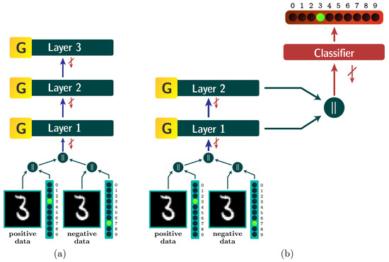
Figure 1.
(a) The architecture of a primitive Forward-Forward Neural Network with 3 dense layers and (b) The architecture of a network where FF layers are used as feature extractors, while the classifier layer is used for output classification. The red crossed-out backward arrows indicate that the updates to the layer do not propagate backwards but are local to that layer itself.
For our experiments, we will only consider two or three hidden dense layers. The classification for a given input image is performed by creating copies of the flattened image tensor concatenated with all possible one-hot output embeddings, running all of them through the network and considering the input tensor with the highest “goodness” as our prediction [4]. Let be the normalized activation vector as described in Equation (4).
The activation of the i-th layer is computed as per Equation (5), where is the layer’s weight matrix, is its bias vector and is the rectified linear unit [18] activation function , where .
2.3. The Forward-Forward Neural Network + Classifier Layer
Another possible architecture we will consider is shown in Figure 1b. This model proves to be very powerful and is a hybrid between the FF layers and a linear classifier layer trained with ordinary cross-entropy loss function. The features that the FF layers can extract are strongly category-specific, allowing the classifier layer to easily classify images with a single forward pass rather than a pass for each specific label like the FFNN. The input of the classifier layer is a concatenation of the outputs of all FF-trained layers as seen in Equation (6), which defines the classification result :
Here, L is the number of FF layers, while and are the weight matrix and bias vector of the classifier layer, respectively.
The training of this network is performed in two steps: First, the FF layers are trained in the fashion of the primitive FFNN for half of the epochs, learning the required features and intrinsically distributing the neurons into category-specific ensembles. After that, the classifier layer is trained for the same number of epochs with a cross-entropy loss function using the features extracted by the FF layers. During the training stage of the classifier, the FF layers are frozen.
2.4. The Forward-Forward Recurrent Neural Network
The Forward-Forward Recurrent Neural Network (FFRNN), shown in Figure 2 and defined by Equations (7) and (8), is inspired by Hinton’s recurrent neural network architecture concept [19] and only made possible by the later introduction of the Forward-Forward algorithm [4]. To solve the limitation of the ordinary Forward-Forward concept, where earlier layers are unable to learn from later layers, we can introduce weights in the backward data-flow direction as well. While forward weights are denoted with blue arrows in Figure 2, backward weights are shown as red arrows. In a Forward-Forward type of neural network, this is possible because each layer learns locally similarly to energy-based models [6,20], and there is no need for error backpropagation.
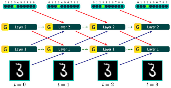
Figure 2.
The diagram of a FFRNN across 4 time steps. The blue arrows represent the forward weights, and the red arrows represent the backward weights. The green arrows represent momentum transfer between time steps, controlled by the hyperparameter. Updates to each layer do not propagate backwards, but are local to the layer itself. The activation of each of the hidden layers is affected by the activation of the layer itself, the activation of the previous layer and the activation of the next layer from the previous time step.
The activation vector of the i-th layer at time t, denoted by , can be calculated as follows:
where and are the forward and backward weights of the i-th layer, respectively, is the bias of the i-th layer and is a momentum coefficient used to transfer information between time steps (green arrows in Figure 2), consequently avoiding biphasic oscillations. The nice property of such a network architecture is that the weights of all layers can be updated in parallel. Even though this might be very useful when using analog hardware or powerful graphic cards with small training batch sizes, our implementation currently does not take advantage of this property.
In our implementation, the activation of the input layer is the flattened input image and the activation of the last layer is the desired one-hot embedding of the corresponding label. At time , activations of each hidden layer are initialized with a uniform random distribution and a single forward pass. After initialization at time , the main iterations follow. Here, we define three hyperparameters, , and . The parameters and are the number of iterations for which we let the image “play out” in the training and the testing phase, respectively, before reinitializing the activations of all layers. However, when making predictions, the first couple of iterations are not yet meaningful due to the time needed for the information from the input and output layers to amalgamate in all of the hidden layers. That is why we only take the sum of the goodness values after the -th iteration, i.e., in the interval of iterations.
2.5. Sparsity Metrics
Naturally, a sparse vector is one in which a small number of components contain a large proportion of the energy [21]. Given a vector , it is useful to define sparsity metrics as functions that quantify how concentrated the energy is among the components. In such metrics, higher values correspond to greater sparsity. Commonly used sparsity metrics are investigated in [21], but we chose to focus only on the ones used by [22] and defined in Equations (9)–(12), with the modification of taking the absolute values of the components, since weight and bias parameters can also be negative. The chosen sparsity metrics give a broader view of the sparsity characteristics of the weight matrices than any single metric alone. They capture different aspects of sparsity, such as the distribution of absolute magnitudes, the influence of large values and the inequality in the distribution of component values relative to their rank.
- -normalized negative entropy is based on information theory and measures how evenly the absolute magnitudes are distributed:
- -normalized negative entropy emphasizes the contribution of larger values:
- The Hoyer sparsity metric combines the and norms:
- The Gini index captures the inequality in the distribution of component values, based on their rank after they are sorted in ascending order:
2.6. Pruning Methodology
Over the years, various pruning methods have been proposed to reduce the complexity of neural networks. In our research, we employ a one-shot static pruning applied post-training and without fine-tuning. This allows us to assess the network’s innate robustness rather than any regularization-induced behavior that might be introduced by applying dropout layers. While more sophisticated approaches such as iterative pruning [23] have also been considered and may yield better empirical results, they introduce additional variables and tuning complexity and are computationally very expensive.
We have implemented different pruning heuristics. Some are based on the neural activations captured over a randomly sampled batch of data, while others rely purely on the weight matrices. All methods produce comparable results, suggesting that FF networks exhibit consistent behavior under different pruning criteria. Ultimately, we focus on a one-shot neuron pruning strategy, which prunes complete neurons rather than individual weight parameters and is defined as follows:
Let denote the number of neurons in layer i, and let be the pruning function that retains t neurons in that layer. A random permutation p of length is generated, and the first t indices () determine the neurons that are preserved in layer i. Rows of the weight matrix and components of the bias vector corresponding to the neurons that will not be preserved in the pruning are completely deleted. Consequently, the later layers are also adapted to the deleted neurons of the previous ones. The described approach guarantees consistency across multiple thresholds t by preserving the subset of neurons when t is increased. The pruning function is applied to each layer independently with the same threshold t.
3. Results
To set the reference for the Forward-Forward-based architectures and obtain the results for this research, we developed the FFLib [16]—a pure Python 3.12.10 library built on top of PyTorch 2.6.0 with CUDA support [24]. FFLib aims to provide a modular and extensible framework along with a suite of tools for training, validating, testing, debugging and experimenting with Forward-Forward models. All of the studied datasets and proposed architectures are implemented in FFLib, which allows extending them and the overall scope to even more complex FF-based or hybrid architectures. Possibilities include adaptation of Convolutional Neural Networks (CNNs) and Graph Neural Networks (GNNs) to the FF-based learning approach with the help of the FFLib architecture and suites [25].
We have conducted several experiments, including the sensitivity analysis of model performance and weight sparsity with respect to the learning rate, loss threshold () and layer size (Section 3.1), visualization of neural activation maps in FF networks in comparison to BPNN and analysis of statistical properties and sparsity of the weight matrices (Section 3.2). We have also evaluated the inverse loss optimization and its effect on baseline performance across FF networks (Section 3.3) and assessed the prunability and robustness of BP and FF networks (Section 3.4). The results are further discussed in Section 4.
All of the experiments were conducted on a workstation equipped with an Intel i9-13900K CPU, 64GB RAM and NVIDIA RTX 4090 GPU. The experiments are based on three different datasets, MNIST [17], FashionMNIST [26] and CIFAR-10 [27], which are widely used benchmark datasets that vary in visual complexity and classification difficulty. These datasets are particularly suitable for evaluating simple MLP architectures. The MNIST [17] dataset consists of 70,000 grayscale images of handwritten digits (0–9), where each imaged is 28 by 28 pixels; FashionMNIST [26] shares the same format but contains grayscale images of 10 categories of clothing items, offering increased visual complexity, and CIFAR-10 [27] is the most difficult dataset that consists of 60,000 color images, each 32 by 32 pixels in size, spanning 10 classes of natural objects such as animals and vehicles. All of the used datasets already include a separation of training and test data; however, we used the last 10% of the training set as a validation set. Since the FFLib [16] manages all of the forementioned datasets internally, our results are easily reproducible.
3.1. Sensitivity Analysis of Sparsity
In this section, we present the results of sensitivity analysis of FF networks. We have tested the effects of hyperparameters, in particular the learning rate and the loss threshold , on network accuracy (Figure 3, Figure 4 and Figure 5) and sparsity (Figure 6, Figure 7 and Figure 8). Learning rate is a crucial hyperparameter that controls the step size during the optimization process [28]. A high learning rate can lead to overshooting of optimal solution, while a low learning rate can result in slow convergence. Understanding how these hyperparameter configurations influence the accuracy, stability and sparsity of the networks is important for ensuring robustness and reproducibility across varying tasks and datasets.
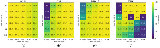
Figure 3.
Sensitivity analysis of the accuracy on the MNIST dataset of (a) BPNN, (b) FFNN, (c) FFNN+C and (d) FFRNN with respect to the learning rate and loss threshold () hyperparameters. The networks were trained to minimize for 60 epochs. The BPNN does not use the loss threshold hyperparameter, so the values in each column are equal for all rows.
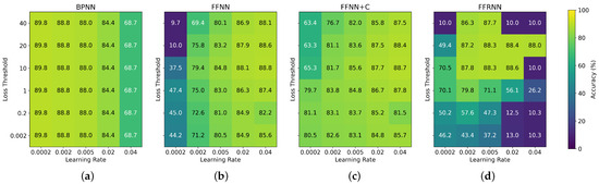
Figure 4.
Sensitivity analysis of the accuracy on the FashionMNIST dataset of (a) BPNN, (b) FFNN, (c) FFNN+C and (d) FFRNN with respect to the learning rate and loss threshold () hyperparameters. The networks were trained to minimize for 60 epochs. The BPNN does not use the loss threshold hyperparameter, so the values in each column are equal for all rows.
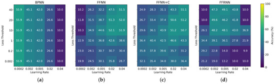
Figure 5.
Sensitivity analysis of the accuracy on the CIFAR-10 dataset of (a) BPNN, (b) FFNN, (c) FFNN+C and (d) FFRNN with respect to the learning rate and loss threshold () hyperparameters. The networks were trained to minimize for 60 epochs. The BPNN does not use the loss threshold hyperparameter, so the values in each column are equal for all rows.
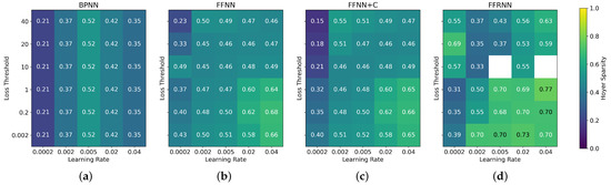
Figure 6.
Sensitivity analysis of the mean Hoyer sparsity of all layers of (a) BPNN, (b) FFNN, (c) FFNN+C and (d) FFRNN with respect to the learning rate and loss threshold () hyperparameters. The heatmap shows the sparsity of the model after training with MNIST dataset. The BPNN does not use the loss threshold hyperparameter, so the heatmap is equal across all rows. The white cells indicate that the training of the model failed to converge in the given configuration.
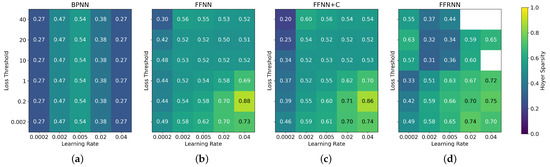
Figure 7.
Sensitivity analysis of the mean Hoyer sparsity of all layers of (a) BPNN, (b) FFNN, (c) FFNN+C and (d) FFRNN with respect to the learning rate and loss threshold () hyperparameters. The heatmap shows the sparsity of the model after training with FashionMNIST dataset. The BPNN does not use the loss threshold hyperparameter, so the heatmap is equal across all rows. The white cells indicate that the training of the model failed to converge in the given configuration.
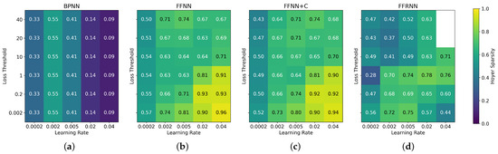
Figure 8.
Sensitivity analysis of the mean Hoyer sparsity of all layers of (a) BPNN, (b) FFNN, (c) FFNN+C and (d) FFRNN with respect to the learning rate and loss threshold () hyperparameters. The heatmap shows the sparsity of the model after training with CIFAR-10 dataset. The BPNN does not use the loss threshold hyperparameter, so the heatmap is equal across all rows. The white cells indicate that the training of the model failed to converge in the given configuration.
In FF networks, the high loss threshold requires the network to change its weights more drastically to be able to classify positive and negative data correctly, which necessitates a higher learning rate for effective optimization. Due to the magnitude of the activations on the input and the loss function, a lower loss threshold leads to worse overall performance of the FF networks, most notably seen in Figure 5. It should be also noted that the more complex FFRNN is especially sensitive to the hyperparameter configuration, which can be seen by the erratic heatmaps in Figure 3d, Figure 4d and Figure 5d.
To ensure visual clarity and conserve space, we report only the Hoyer sparsity metric in this section. It effectively captures the balance between the and norms and is used in related literature [7,9]. The analysis of how model hyperparameters influence sparsity, presented in Figure 6, Figure 7 and Figure 8, shows that all of the FF architectures exhibit Hoyer sparsity higher than 0.4 in almost every configuration. This suggests that the training of MLPs using the FF algorithm leads to sparse weight matrices regardless of the loss threshold and learning rate hyperparameters. We previously assumed that the learning rate of the BPNN and the sparsity of its weights are positively correlated. However, this may not be the case, as the sparsity peaks at a learning rate of 0.005 and decreases again as the learning rate increases further. Finally, in the case of FFRNN, a high learning rate can lead to less stable training and fail to converge, which is marked by the white cells in Figure 6d, Figure 7d and Figure 8d.
To analyze the impact of layer size on the sparsity of the weight matrices in FFNN networks compared to BPNN, we monitored the sparsity progression during training across multiple layer sizes. The layer sizes were varied from 50 to 4000 neurons per layer. The resulting graphs of -normalized negative entropy, -normalized negative entropy, Hoyer sparsity and Gini sparsity are presented in Figure 9, Figure 10, Figure 11 and Figure 12, respectively. As expected, all of the metrics show a clear gap between the sparsity in FFNN and BPNN. Furthermore, the Hoyer and Gini sparsity change very little for different layer sizes, indicating that the sparsity characteristics are not significantly influenced by the neuron count. The inverse logarithmic factor in and entropy-based metrics leads to ostensibly higher sparsity values at lower layer sizes, which makes them less suitable for analyzing the effects of different layer sizes.
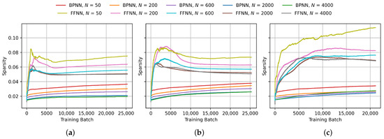
Figure 9.
Progression of -normalized negative entropy of the weight matrices during BPNN and FFNN training on (a) MNIST, (b) FashionMNIST and (c) CIFAR-10 with different layer sizes. N indicates the number of neurons in each of the two hidden layers.
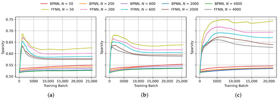
Figure 10.
Progression of -normalized negative entropy of the weight matrices during BPNN and FFNN training on (a) MNIST, (b) FashionMNIST and (c) CIFAR-10 with different layer sizes. N indicates the number of neurons in each of the two hidden layers.
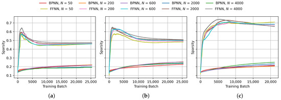
Figure 11.
Progression of Hoyer sparsity of the weight matrices during BPNN and FFNN training on (a) MNIST, (b) FashionMNIST and (c) CIFAR-10 with different layer sizes. N indicates the number of neurons in each of the two hidden layers.
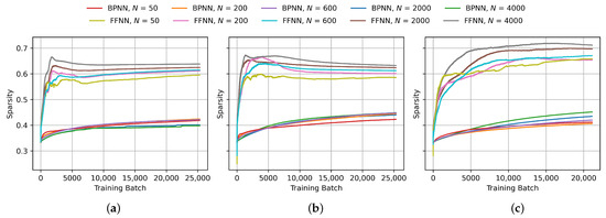
Figure 12.
Progression of Gini sparsity of the weight matrices during BPNN and FFNN training on (a) MNIST, (b) FashionMNIST and (c) CIFAR-10 with different layer sizes. N indicates the number of neurons in each of the two hidden layers.
In order to conduct all of the next experiments, we have used a fixed set of hyperparameter values, provided in Table 1. The baseline accuracies of all models achieved on the different datasets are shown in Table 2. The achieved accuracies do not differ much from what is commonly reported for MLP benchmarks on these datasets. While the BPNN outperforms all other networks on all datasets, the margin is quite small on MNIST and FashionMNIST. The FFRNN even achieved accuracy on MNIST, which is the best among all FF-trained networks and close to what is reported by Hinton [4].

Table 1.
Training hyperparameters for all networks. Hyperparameters that do not apply for some architectures are denoted with N/A.
Table 2.
The mean and standard deviation of test accuracy (%) over 10 independent training runs of BPNN, FFNN, FFNN+C, and FFRNN on the MNIST, FashionMNIST and CIFAR-10 datasets.
3.2. Structural and Functional Sparsity Analysis
Prior studies [7,9] have shown that FF networks exhibit sparse activations when inferred. Our experiments support these findings, as demonstrated by Figure 13, which shows sparse activations when the same single sample from the MNIST dataset is processed by all of the implemented networks. The activation maps are normalized on a per-layer basis. It can be seen that all of the FF networks exhibit higher activation sparsity compared to the BPNN, as witnessed by a larger number of dark pixels in the FF models’ activation maps.
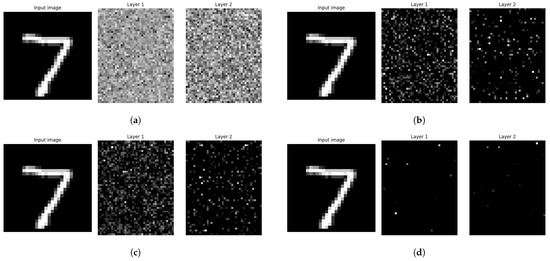
Figure 13.
Activation maps for the same input sample, visualized across different architectures: (a) BPNN, (b) FFNN, (c) FFNN+C and (d) FFRNN. The activations are normalized for each layer separately, where black indicates the lowest and white the highest activation of a single neuron.
We have extended the sparsity analysis to include the functional sparsity, i.e., the property of the model to activate only a small number of typically specialized units per input class. Figure 14 shows the accumulated activation maps over a batch of input samples, visualized in the HSV color space. The hue in the figure represents the class label that the neuron is most responsive to, the saturation indicates the specialization of the neuron to that class and the brightness conveys the average activation strength. The HSV visualization clearly demonstrates both the higher sparsity and higher specialization of neurons to specific classes in the FF networks compared to the BPNN. While the BPNN maps are mostly grey, indicating that a lot of neurons are active most of the time and are not specialized to any specific class, the FFNN and FFRNN exhibit a more pronounced specialization that can be seen in neural ensembles with high saturation and distinct hues.
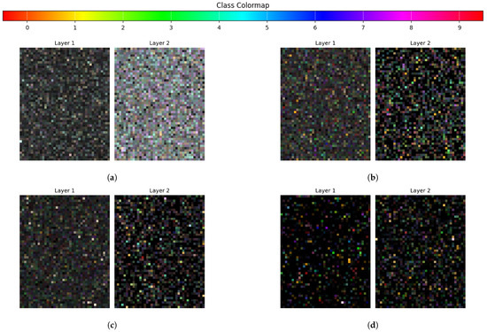
Figure 14.
Accumulated activation maps over a batch of samples, visualized in the HSV color space across different architectures: (a) BPNN, (b) FFNN, (c) FFNN+C and (d) FFRNN. Hue represents the class label that the neuron is most responsive to, saturation indicates the specialization of the neuron to that class and value represents the average activation strength.
From the perspective of neural network prunability, our interest is in the structural sparsity of the weight matrices and bias vectors of each layer. For that purpose, we ran the experiments to capture the progression of sparsity of the weight matrices of each layer throughout the training process, as shown in Figure 15, Figure 16, Figure 17 and Figure 18. From the figures, a significant increase in structural sparsity can be observed in the early training phases of the FFNN compared to the BPNN. The graphs show that even from the start of the training process, a smaller portion of the weights becomes responsible for most of the energy in the FFNN compared to the BPNN. The peak could be attributed to the contrastive nature of the FF algorithm, where even from the beginning of the training process, the FF algorithm tries to improve the contrast between positive and negative data, immediately trying to specialize neurons into class-based ensembles, as seen in Figure 14.
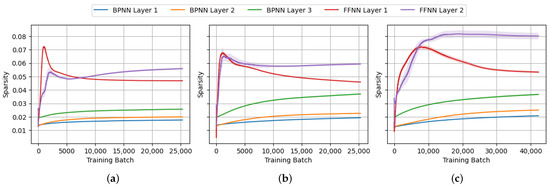
Figure 15.
The progression of -normalized negative entropy of the weight matrices during BPNN and FFNN training on (a) MNIST, (b) FashionMNIST and (c) CIFAR-10.
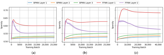
Figure 16.
The progression of -normalized negative entropy of the weight matrices during BPNN and FFNN training on (a) MNIST, (b) FashionMNIST and (c) CIFAR-10.
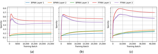
Figure 17.
The progression of Hoyer sparsity of the weight matrices during BPNN and FFNN training on (a) MNIST, (b) FashionMNIST and (c) CIFAR-10.
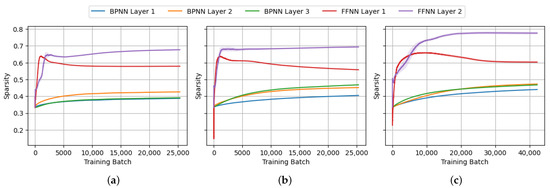
Figure 18.
The progression of Gini sparsity of the weight matrices during BPNN and FFNN training on (a) MNIST, (b) FashionMNIST and (c) CIFAR-10.
The structural sparsity for all of the fully trained FFNN and BPNN is presented in Table 3. The mean and standard deviation of 10 independent runs with different seeds are reported. It can be seen that the training of the FFNN forms sparser weight matrices in all scenarios with respect to all four sparsity metrics. The standard deviation is orders of magnitude lower than the mean, which suggests that random weight initialization has no major effect on final weight sparsity. The imbalance in how much each layer contributes to the network’s function in FFNNs leads to greater differences in structural sparsity across layers, compared to BPNNs.
Table 3.
The mean and standard deviation of post-training weight sparsity for BPNN and FFNN, averaged over 10 independent runs with different seeds and fixed hyperparameters from Table 1. For clarity, all values are rounded to three decimal places; a standard deviation of 0.000 indicates a value less than 0.0005.
The statistical properties of weight matrices for different architectures and layers were also analyzed, and the results are shown in Table 4. In the table, FFNN2 and FFNN3 refer to the same architecture described in Section 2.2 with the difference that FFNN3 has three hidden layers with 2000 neurons each, while FFNN2 has only two layers. Experiments were conducted for both loss functions, and , in FF-based networks, and the cross-entropy (CE) loss in BPNN, showing the range, mean and standard deviation of the values in the weight matrices across all layers. The difference between the weight ranges of trained BPNN- and FF-based networks is conspicuous. While the BPNN maintains similar weight distribution across all layers, the difference is more pronounced in the FF networks.
Table 4.
Statistics for the weight matrices of different network types trained on the MNIST dataset.
3.3. Inverse Optimization
The goal of the next experiment was to answer whether to maximize the neural activations for positive data () or to invert the optimization and optimize for . We trained 10 randomly initialized instances of FF networks on the MNIST dataset using both loss functions (see Equations (2) and (3)) and measured their post-training accuracy. We then performed an independent two-sample t-test to compare the accuracy of networks trained with either loss function. The null hypothesis was that there was no significant difference in performance between and . The obtained results are shown in Table 5. It was found that the optimization for is statistically significantly better than for in the case of larger networks (FFRNN and FFNN3). We believe that the reason is in the way the negative data is generated (see Section 2.1), which results in a higher variance of the control vector for negative data than for positive, making it easier for the Adam optimizer [28] to find better minima when optimizing for .
Table 5.
The comparison of the test accuracies achieved using the loss functions and in FF networks trained on MNIST.
3.4. Prunability
Prunability refers to the network’s ability to retain its accuracy even when a significant fraction of its parameters or entire neurons are removed [29]. To evaluate the native robustness and prunability of FF-based networks, we applied the methodology described in Section 2.6. We conducted the prunability tests on all described FF architectures on three different datasets, MNIST [17], FashionMNIST [26] and CIFAR-10 [27], and obtained the results shown in Figure 19a, Figure 19b and Figure 19c, respectively. The compression ratio on all graphs is defined as per Equation (13).
where the size of the pruned model is measured after applying the pruning methodology described in Section 2.6 for a fixed list of exponentially decreasing values for the parameter t. Each curve in the plots represents the mean classification accuracy over 10 independent runs, each with a different random seed. Shaded areas depict one standard deviation, and dashed lines indicate the observed minimum and maximum accuracies. These plots capture not only the average performance under pruning, but also the variance and worst-case robustness of each model configuration. From the data presented on Figure 19, it can be observed that the simple FFNN architecture, whose accuracy curve is plotted in green, is noticeably more robust trained on all three datasets when compared to the other more complex architectures. The lower performance of the FFNN+C indicates that the Classifier layer is substantially crippling the network’s performance and suggests that a more complex Classifier block is required to maintain the level of robustness seen in FFNN. The FFRNN’s architecture is substantially more intertwined than the others, leading to better maximum performance but lower robustness that indicates that a larger part of the neurons are important to the classification compared to that of the other networks. It is also worth noting that, in the case of CIFAR-10, the FFNN exhibits a higher variance of accuracy, as reflected by the large standard deviation in Figure 19c. We believe that this is due to the fact that the CIFAR-10 dataset is more complex than the other two datasets with greater intra-class data variability.
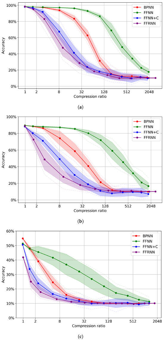
Figure 19.
Prunability of different networks trained on (a) MNIST, (b) FashionMNIST and (c) CIFAR-10 where FF-based networks are trained to minimize the neural activations for positive data.
4. Discussion
To provide the foundations for the pruning experiments, we have conducted several experiments focusing on the sparsity of FF networks. The sensitivity and sparsity analysis conducted in Section 3.1 and Section 3.2 uncovered the structural and functional sparsity characteristics of FFNN compared to BPNN. We showed that the structural sparsity is considerably larger in FF-based networks than in the BP-based ones even when many hyperparameters are adjusted. We suggest that the contrastive loss in FF networks encourages layers to rapidly adopt sparse configurations. The HSV visualization for the neural specialization and class dependence further demonstrated that the sparsity in FF networks is not only structural, but also functional. The individual neural activations are considerably more specialized to specific classes across all FF networks.
The statistical analysis of trained model parameters revealed that the ranges of weight values tend to be significantly wider in the case of FF networks than in the BP-trained models (Table 4). This can be attributed to the two properties of our Forward-Forward algorithm implementation, a relatively high loss threshold and high learning rates, which are specific to the goodness activation function.
In all FF models, particularly FFNN and FFNN+C, we observe that the range of values and the standard deviation of the weight matrix are typically higher in the first layer compared to subsequent layers. This suggests that earlier layers undergo more aggressive updates, potentially due to substantial partitioning of the vector space in the first layer, diminishing the contribution of later layers.
In contrast, FFRNN expresses a more balanced weight distribution across layers, likely due to the recurrent connections facilitating some degree of internal feedback. In the case of the proposed FFRNN architecture, the entire network acts like a single layer that corrects itself over time. This behavior supports the hypothesis proposed in [19] that the FF models with internal recurrence or lateral connections are better suited to form hierarchical representations.
As also noted by Hinton [4], the FF networks generally converge more slowly than their backpropagation-trained counterparts, owing to their lack of global coordination during training. Despite this, our experiments show that FF models can achieve comparable baseline accuracy to BP models across MNIST, FashionMNIST and CIFAR-10 (Table 5), which allows pruning experiments on all networks across all datasets.
FFNN exhibits remarkable resilience to random neuron pruning, achieving up to 8× compression with minimal loss in performance on MNIST and FashionMNIST. On the other hand, when trained on CIFAR-10, FFNN shows a high variance in accuracy across different pruning levels (Figure 19c) and also a rapid decline after pruning, which is, however, even faster with BPNN.
We have also experimented with a simple activation-based pruning heuristic, where neuron activations from a randomly sampled batch are used to sort and remove the least active neurons. This heuristic, when applied to FFRNN, yielded a performance comparable to or better than that of BPNN when evaluated under the random one-shot pruning approach from Section 2.6. Interestingly, when the same heuristic is applied to the BPNN, the performance of the BPNN drops significantly, making it perform worse than all FF architectures.
Finally, we observed that threshold-based pruning of individual weights, independent of neural structure, produces nearly identical trends across all architectures, regardless of their complexity or size. This suggests that structural properties and subsets, rather than individual weights, may play a more decisive role in FF networks’ robustness to pruning.
5. Conclusions
In the paper, we explore the prunability of multi-layer perceptrons trained using the Forward-Forward (FF) algorithm and compare them to a dense MLP network trained with the backpropagation algorithm (BP). Our results show that the FF-based MLP networks are indeed way more robust to one-shot random neuron pruning than their BP counterparts, achieving similar accuracy with significantly fewer active neurons. The FFNN maintained accuracy even after aggressive pruning, particularly on simpler datasets like MNIST and FashionMNIST. However, more complex FF networks with additional classification layers and FFRNNs have many more internal structures that are tightly connected and exhibit worse performance than ordinary BP MLP when subjected to one-shot pruning.
FFNN’s good performance after random neuron pruning might contribute the right characteristics not only for resource-constrained devices like IoT hardware, where memory and computing limitations make model size critical, but also for robustness against hardware failures.
While our study offers new insights into the sparsity and prunability of neural networks trained with the FF algorithm, it is not without its limitations. In particular, it is limited to the MNIST, FashionMNIST and CIFAR-10 datasets. Additional experiments are required to determine the characteristics of FF networks trained on larger and more complex datasets, especially in non-visual modalities. Moreover, the sparsity benefits of FF may not be as pronounced in more complex neural network architectures, such as CNNs or GNNs. With regard to the study of the prunability, the presented methodology can be extended with heuristic pruning strategies tailored to the specific architectures and datasets.
A new field of neural research that was spurred by the introduction of the Forward-Forward algorithm raised many yet-to-be answered questions. Future work could explore the following:
- Comparing the performance of the architectures with and without fine-tuning after the pruning procedure.
- Researching the possibility of using techniques, such as quantization, knowledge distillation or low-rank factorization, on FF networks to achieve even smaller model sizes.
- How does adding regularization, such as peer normalization loss, affect the sparsity, performance and pruning outcomes?
- How robust are CNNs trained with the FF algorithm under pruning?
- What is the true compressibility of FF networks when the methodology is extended with compression algorithms such as ZIP, LZMA or arithmetic coding?
Author Contributions
Conceptualization, M.N. and D.S.; methodology, M.N. and D.S.; software, M.N.; validation, D.S. and D.P.; formal analysis, M.N. and D.S.; investigation, M.N. and D.P.; resources, D.P.; data curation, M.N.; writing—original draft preparation, M.N.; writing—review and editing, D.S. and D.P.; visualization, M.N.; supervision, D.S. and D.P.; project administration, D.S. and D.P.; funding acquisition, D.P. All authors have read and agreed to the published version of the manuscript.
Funding
This research was funded by the Slovene Research and Innovation Agency under Research Project J2-4458 and Research Programme P2-0041.
Data Availability Statement
The source code for all of the neural networks and experiments is available at https://github.com/mitkonikov/ff-research (accessed on 14 August 2025). It is based on FFLib, which is available at https://github.com/mitkonikov/ff (accessed on 14 August 2025).
Conflicts of Interest
The authors declare no conflicts of interest. The funders had no role in the design of the study; in the collection, analyses, or interpretation of data; in the writing of the manuscript; or in the decision to publish the results.
Abbreviations
The following abbreviations are used in this manuscript:
| BP | Backpropagation Algorithm |
| BPNN | Backpropagation Neural Network |
| CE | Cross-Entropy Loss |
| CIFAR | Canadian Institute for Advanced Research |
| CNN | Convolutional Neural Network |
| CUDA | Compute Unified Device Architecture |
| FF | Forward-Forward Algorithm |
| FFNN | Forward-Forward Neural Network |
| FFNN2 | Forward-Forward Neural Network with 2 Layers |
| FFNN3 | Forward-Forward Neural Network with 3 Layers |
| FFNN+C | Forward-Forward Neural Network + Classifier |
| FFRNN | Forward-Forward Recurrent Neural Network |
| GNN | Graph Neural Network |
| HSV | Hue Saturation Value |
| IoT | Internet of Things |
| LZMA | Lempel-Ziv-Markov Chain Algorithm |
| MLP | Multi-Layer Perceptron |
| MNIST | Modified National Institute of Standards and Technology |
References
- Rumelhart, D.E.; Hinton, G.E.; Williams, R.J. Learning representations by back-propagating errors. Nature 1986, 323, 533–536. [Google Scholar] [CrossRef]
- Hochreiter, S. Untersuchungen zu Dynamischen Neuronalen Netzen. Master’s Thesis, Technische Universitat, Munchen, Germany, 1991. Volume 91. p. 31. [Google Scholar]
- Bengio, Y.; Simard, P.; Frasconi, P. Learning long-term dependencies with gradient descent is difficult. IEEE Trans. Neural Netw. 1994, 5, 157–166. [Google Scholar] [CrossRef] [PubMed]
- Hinton, G. The Forward-Forward Algorithm: Some Preliminary Investigations. arXiv 2022, arXiv:2212.13345. [Google Scholar] [CrossRef]
- Carreira-Perpinan, M.A.; Hinton, G. On contrastive divergence learning. In International Workshop on Artificial Intelligence and Statistics; PMLR: Bridgetown, Barbados, 2005; pp. 33–40. [Google Scholar]
- Hinton, G.E.; Sejnowski, T.J. Learning and relearning in Boltzmann machines. Parallel Distrib. Process. Explor. Microstruct. Cogn. 1986, 1, 282–317. [Google Scholar]
- Tosato, N.; Basile, L.; Ballarin, E.; Alteriis, G.D.; Cazzaniga, A.; Ansuini, A. Emergent representations in networks trained with the Forward-Forward algorithm. Trans. Mach. Learn. Res. 2025. Available online: https://openreview.net/forum?id=JhYbGiFn3Y (accessed on 14 August 2025).
- Miller, J.e.K.; Ayzenshtat, I.; Carrillo-Reid, L.; Yuste, R. Visual stimuli recruit intrinsically generated cortical ensembles. Proc. Natl. Acad. Sci. USA 2014, 111, E4053–E4061. [Google Scholar] [CrossRef] [PubMed]
- Yang, Y. A theory for the sparsity emerged in the Forward Forward algorithm. arXiv 2023, arXiv:2311.05667. [Google Scholar] [CrossRef]
- Gandhi, S.; Gala, R.; Kornberg, J.; Sridhar, A. Extending the Forward Forward Algorithm. arXiv 2023, arXiv:2307.04205. [Google Scholar] [CrossRef]
- Giampaolo, F.; Izzo, S.; Prezioso, E.; Piccialli, F. Investigating Random Variations of the Forward-Forward Algorithm for Training Neural Networks. In Proceedings of the 2023 International Joint Conference on Neural Networks (IJCNN), Gold Coast, Australia, 18–23 June 2023; pp. 18–23. [Google Scholar] [CrossRef]
- Ororbia, A.; Mali, A. The Predictive Forward-Forward Algorithm. arXiv 2023, arXiv:2301.01452. [Google Scholar] [CrossRef]
- Chen, X.; Liu, D.; Laydevant, J.; Grollier, J. Self-Contrastive Forward-Forward Algorithm. Nat. Commun. 2025, 16, 5978. [Google Scholar] [CrossRef] [PubMed]
- Ghader, M.; Reza Kheradpisheh, S.; Farahani, B.; Fazlali, M. Enabling Privacy-Preserving Edge AI: Federated Learning Enhanced with Forward-Forward Algorithm. In Proceedings of the 2024 IEEE International Conference on Omni-layer Intelligent Systems (COINS), London, UK, 29–31 July 2024; pp. 1–7. [Google Scholar] [CrossRef]
- Reyes-Angulo, A.A.; Paheding, S. Forward-Forward Algorithm for Hyperspectral Image Classification. In Proceedings of the 2024 IEEE/CVF Conference on Computer Vision and Pattern Recognition Workshops (CVPRW), Seattle, WA, USA, 16–22 June 2024; pp. 3153–3161. [Google Scholar] [CrossRef]
- Nikov, M. FFLib: Forward-Forward Neural Networks Library. 2025. Available online: https://github.com/mitkonikov/ff (accessed on 14 August 2025).
- Deng, L. The mnist database of handwritten digit images for machine learning research. IEEE Signal Process. Mag. 2012, 29, 141–142. [Google Scholar] [CrossRef]
- Householder, A.S. A Theory of Steady-State Activity in Nerve-Fiber Networks: I. Definitions and Preliminary Lemmas. Bull. Math. Biophys. 1941, 3, 63–69. [Google Scholar] [CrossRef]
- Hinton, G. How to represent part-whole hierarchies in a neural network. arXiv 2021, arXiv:2102.12627. [Google Scholar] [CrossRef] [PubMed]
- Huang, Y.; Rao, R.P. Predictive coding. Wiley Interdiscip. Rev. Cogn. Sci. 2011, 2, 580–593. [Google Scholar] [CrossRef] [PubMed]
- Hurley, N.; Rickard, S. Comparing measures of sparsity. IEEE Trans. Inf. Theory 2009, 55, 4723–4741. [Google Scholar] [CrossRef]
- Kuzma, T.; Farkaš, I. Computational analysis of learned representations in deep neural network classifiers. In Proceedings of the 2018 International Joint Conference on Neural Networks (IJCNN), Rio de Janeiro, Brazil, 8–13 July 2018; pp. 1–8. [Google Scholar]
- Frankle, J.; Carbin, M. The Lottery Ticket Hypothesis: Finding Sparse, Trainable Neural Networks. arXiv 2019, arXiv:1803.03635. [Google Scholar] [CrossRef]
- Ansel, J.; Yang, E.; He, H.; Gimelshein, N.; Jain, A.; Voznesensky, M.; Bao, B.; Bell, P.; Berard, D.; Burovski, E.; et al. PyTorch 2: Faster Machine Learning Through Dynamic Python Bytecode Transformation and Graph Compilation. In Proceedings of the 29th ACM International Conference on Architectural Support for Programming Languages and Operating Systems, Volume 2 (ASPLOS ’24), San Diego, CA, USA, 27 April–1 May 2024. [Google Scholar] [CrossRef]
- Scodellaro, R.; Kulkarni, A.; Alves, F.; Schröter, M. Training Convolutional Neural Networks with the Forward-Forward algorithm. arXiv 2024, arXiv:2312.14924. [Google Scholar] [CrossRef]
- Xiao, H.; Rasul, K.; Vollgraf, R. Fashion-MNIST: A Novel Image Dataset for Benchmarking Machine Learning Algorithms. arXiv 2017, arXiv:1708.07747. [Google Scholar] [CrossRef]
- Krizhevsky, A.; Nair, V.; Hinton, G. CIFAR-10 and CIFAR-100 (Canadian Institute for Advanced Research). 2009. Available online: http://www.cs.toronto.edu/~kriz/cifar.html (accessed on 14 August 2025).
- Kingma, D.P.; Ba, J. Adam: A Method for Stochastic Optimization. In Proceedings of the 3rd International Conference on Learning Representations, ICLR 2015, San Diego, CA, USA, 7–9 May 2015. [Google Scholar]
- Ankner, Z.; Renda, A.; Dziugaite, G.K.; Frankle, J.; Jin, T. The Effect of Data Dimensionality on Neural Network Prunability. arXiv 2022, arXiv:2212.00291. [Google Scholar] [CrossRef]


Disclaimer/Publisher’s Note: The statements, opinions and data contained in all publications are solely those of the individual author(s) and contributor(s) and not of MDPI and/or the editor(s). MDPI and/or the editor(s) disclaim responsibility for any injury to people or property resulting from any ideas, methods, instructions or products referred to in the content. |
© 2025 by the authors. Licensee MDPI, Basel, Switzerland. This article is an open access article distributed under the terms and conditions of the Creative Commons Attribution (CC BY) license (https://creativecommons.org/licenses/by/4.0/).