Abstract
Enterprise bankruptcy prediction is a critical task in financial risk management. Traditional methods, such as logistic regression and decision trees, rely heavily on structured financial data, which limits their ability to capture complex relational networks and unstructured industry information. Heterogeneous graph neural networks (HGNNs) offer a solution by modeling multiple relationships between enterprises. However, current models struggle with financial risk graph data challenges, such as the oversimplification of internal financial features and the lack of dynamic imputation for missing external topological features. To address these issues, we propose HGNN-EBP, an enterprise bankruptcy prediction algorithm that integrates both internal and external features. The model constructs a multi-relational heterogeneous graph that combines structured financial data, unstructured textual information, and real-time industry data. A multi-scale graph convolution network captures diverse relationships, while a Transformer-based self-attention mechanism dynamically imputes missing external topological features. Finally, a multi-layer perceptron (MLP) predicts bankruptcy probability. Experimental results on a dataset of 32,459 Chinese enterprises demonstrate that HGNN-EBP outperforms traditional models, especially in handling relational diversity, missing features, and dynamic financial risk data.
Keywords:
enterprise bankruptcy prediction; heterogeneous graph neural network; Transformer attention mechanism; graph convolutional network MSC:
68T07
1. Introduction
Enterprise bankruptcy prediction is a critical research topic in the field of financial risk management, as it directly influences decisions made by banks, investment institutions, and policymakers. With the rising global enterprise bankruptcy rates (over a 20% increase in bankruptcy rates in Europe and North America in 2024), traditional bankruptcy prediction methods face increasing challenges. These traditional approaches typically rely on financial data of the firm and employ simple statistical models, such as the Altman Z-score [1,2,3], to assess bankruptcy risk. However, these methods are often limited to singular financial data, making it difficult to capture the complex network relationships between firms and external environmental factors. As a result, they perform poorly when faced with the dynamic and complex nature of enterprise risk.
Heterogeneous graph neural networks (HGNN) [4,5,6], as an emerging deep learning approach, effectively integrate multi-source heterogeneous data through graph structures, enabling the modeling of complex, multi-layered relationships between firms and capturing potential risks that influence enterprise bankruptcy. Please refer to Table 1 for details. However, existing HGNN models still face two significant technical bottlenecks when applied to enterprise bankruptcy prediction:

Table 1.
Comparison of core limitations in enterprise bankruptcy prediction method.
1. Shallow Internal Attribute Mining: Many existing models rely on shallow, fully connected layers to process a firm’s financial data, failing to capture the nonlinear patterns and higher-order relationships embedded within the financial data.
2. Static External Feature Imputation: External relationship data between firms (e.g., supply chain, shareholder relationships, etc.) are often incomplete, and traditional imputation methods (such as mean imputation) fail to effectively capture the latent structural information in the missing data. This results in increased errors and severely distorts the risk transmission paths.
To overcome these bottlenecks, this paper proposes a heterogeneous graph neural network-based internal and external feature fusion enterprise bankruptcy prediction model (HGNN-EBP). The core innovations of this model are reflected in the following aspects:
1. Deep Internal Attribute Extraction and Multi-Scale Graph Convolution: Unlike traditional financial data processing methods, HGNN-EBP employs a multi-scale graph convolutional network (GCN) structure to deeply mine the financial data of enterprises. Through multi-level information aggregation, the model not only captures the structural information within the enterprise (such as cash flow, debt ratio, and other financial features), but also uncovers complex nonlinear patterns related to the enterprise’s operational health. This deep feature extraction significantly enhances the model’s ability to perceive enterprise risks, avoiding the traditional dependence on single linear relationships.
2. Dynamic External Feature Reconstruction: To address the missing external relationship data, this paper designs an external feature completion module based on the Transformer attention mechanism. By introducing a neighborhood node adaptive weighting mechanism, the model can effectively complete missing external features (such as undisclosed supplier risks, shareholder relationships, etc.) within the topological relationships between enterprises. Moreover, the model uses a heterogeneous graph attention mechanism to model risk transmission paths across industries, further enhancing its ability to capture complex external environments and multi-layered relationships. This innovation greatly improves the prediction accuracy when external data is missing between enterprises and enhances the model’s ability to identify bankruptcy risks.
3. Internal and External Feature Fusion and Collaborative Optimization: In traditional methods, internal financial features and external relationship features are often processed separately, without fully utilizing the interactive information between the two. To address this limitation, HGNN-EBP introduces an internal and external feature fusion mechanism, collaboratively optimizing internal financial features and external topological features through concatenation. Based on the fused features, the model uses a multi-layer perceptron (MLP) to predict bankruptcy probabilities, significantly improving prediction accuracy. This design breaks through the limitations of traditional models in handling attribute and relationship coupling, providing a more comprehensive and efficient risk assessment capability.
Through these innovations, HGNN-EBP is able to comprehensively consider multi-dimensional enterprise features and provide accurate bankruptcy risk assessments in the face of complex enterprise relationships and external environments. To validate the model’s effectiveness, experiments were conducted on a multi-source dataset. The results show that HGNN-EBP outperforms other models in various evaluation metrics (such as AUC, F1 score, etc.), particularly in modeling complex supply chain relationships and industry risk transmission, demonstrating significant advantages.
This study is organized into seven chapters: Section 1 introduces the academic background of enterprise bankruptcy prediction and the existing technological bottlenecks; Section 2 provides a comprehensive review of the current research on heterogeneous graph neural networks and dynamic feature completion techniques; Section 3 defines the relevant technical concepts and research background; Section 4 presents a detailed explanation of the architecture design and algorithm implementation of the proposed HGNN-EBP model; Section 5 conducts comparative experiments and interpretability analysis using multi-source datasets to validate the model’s performance; Section 6 provides an in-depth discussion of the model’s performance and related issues; and Section 7 summarizes the contributions of this study and outlines future directions, including federated learning and temporal evolution modeling. This progressive structure ensures both theoretical depth and enhances the practical value of the research outcomes.
2. Related Work
2.1. Enterprise Risk Analysis
Traditional enterprise risk analysis primarily relies on financial indicators, such as profitability, operational efficiency, and solvency, combined with multiple discriminant analysis [9,10,11] or machine learning methods (e.g., support vector machines [12] and decision trees [13]) for risk prediction. In recent years, research has gradually shifted toward leveraging textual information to mine internal enterprise risks, such as identifying potential risk signals from unstructured data like conference call transcripts and financial reports. However, small and medium-sized enterprises often lack standardized financial disclosures and public textual data, limiting the applicability of such methods. Meanwhile, external risk sources like litigation, though highly correlated with enterprise credit risk, remain underexplored and underutilized in existing studies.
Contagious enterprise risk [14,15,16] is equally significant, as it reflects the mutual influence of enterprises within complex networks. Existing studies have assessed systemic risk by modeling interbank loan networks, payment networks, etc., revealing that the interconnected structure among enterprises plays a crucial role in risk propagation. Some studies also employ game theory, attention networks, and other methods to simulate the diffusion of risk among enterprises. However, most current research still relies on simulation techniques, making direct application to real-world business scenarios challenging, and few works simultaneously address the integrated modeling of internal and contagious enterprise risks.
2.2. Graph Neural Networks
Graph neural networks (GNNs) leverage deep learning techniques to achieve representation learning for graph-structured data, demonstrating strong performance in tasks such as node classification, link prediction, and graph classification. Meanwhile, GNNs [17,18,19,20] have been widely applied in recommendation systems, natural language processing, and computer vision. In the field of fintech, the complex relationships between enterprises and individuals can be constructed as heterogeneous graphs, and GNN [21,22,23] is used to model various financial risk scenarios. For instance, SemiGNN [24] employs multi-view data for fraud detection; Pu et al. [25] combine rich node and edge attributes to identify loan default risks; Cheng et al. [26] introduce an inter-chain temporal attention mechanism to assess contagion risks in bank guarantee chains; Wasi et al. [27] perform trend prediction based on supply chain graphs; Huang et al. [28] utilize multi-layer attention networks to enhance bankruptcy prediction; and Bi et al. [29] integrate shareholder information and financial news to construct structured graph networks for risk assessment. Additionally, Zhao et al. [30] propose a graph-based deep reinforcement learning method to identify critical nodes in banking systems for controlling risk diffusion. It is worth noting that recent advances in natural language processing (NLP) have significantly improved feature extraction from financial texts: Transformer-based pre-trained models (e.g., FinBERT [31], RoBERTa-Fin [32]), through domain-adaptive training, can effectively capture semantic features in financial reports, news, and social media. Meanwhile, attention-enhanced bidirectional LSTM [33] and hierarchical neural networks [34] have demonstrated strong performance in financial sentiment analysis and event extraction tasks. The integration of these NLP techniques with GNNs (e.g., text-enhanced graph representation learning [35]) has further boosted the accuracy of financial risk prediction.
In recent years, pioneering studies have implemented GNN-based approaches in financial networks. For example, He et al. [36] propose a high-order graph attention representation method to infer systemic credit risks based on inter-company guarantee networks. Shumovskaia et al. [37] develop a GNN model based on recurrent neural networks to explore transaction networks between banks and clients. However, no research has yet applied GNN-based methods to financial heterogeneous information networks (HINs).
Hypergraphs, due to their ability to model high-order relationships, have been widely used in graph classification and computer vision. For instance, the MKHG [38] model proposed by Zeng et al. effectively integrates multi-source heterogeneous information. In enterprise risk analysis, the complex many-to-many relationships between enterprises and associated individuals make hypergraphs suitable for modeling. However, research applying hypergraph neural networks to this domain remains limited. In summary, although various graph models have been employed for enterprise risk identification, few studies simultaneously incorporate internal risks and contagion risks. Moreover, the diversity of risk sources and complexity of relationships make it challenging for many methods to fully uncover latent information. Additionally, the scarcity of publicly available datasets has somewhat hindered progress in this field.
2.3. Heterogeneous Graph Neural Networks
Graph neural networks (GNNs) model the information propagation process between nodes through deep learning methods. Early research primarily focused on modeling homogeneous graphs, but real-world networks are typically composed of heterogeneous graphs, containing different types of nodes and edges. Therefore, current research increasingly emphasizes heterogeneous graph modeling. For example, the RGCN [39] model proposed by Chen et al. employs different relational mapping matrices to handle complex knowledge graphs; the HGT [40] algorithm proposed by et al. is designed for large-scale heterogeneous graph network modeling. MM-GNN [41] utilizes multi-order moments to compute neighbor information distributions and integrates this information via attention mechanisms. Other works include heterogeneous hierarchical attention mechanisms that generate future neighbor node representations based on historical information, as well as contrastive learning-based heterogeneous graph network modeling.
However, existing studies rarely consider both internal enterprise risks and contagious risks simultaneously, and most fail to fully exploit fine-grained contagion risk information. Moreover, the scarcity of publicly available datasets has hindered progress in this field. To better understand and predict enterprise bankruptcy risks, it is necessary to develop a comprehensive model capable of capturing both internal and external risk factors.
3. Definitions and Problem
Definition 1 Enterprise Multi-Relation Heterogeneous Graph.
An enterprise multi-relation heterogeneous graph (Heterogeneous Graph for Multi-Relations in Enterprises) is a graph structure capable of representing multi-dimensional, multi-type relationships among enterprises. Let the graph be denoted as , where is the node set, and is the edge set. Different types of nodes represent distinct entities (e.g., enterprises, suppliers, financial institutions), while different types of edges signify diverse relationships between entities (e.g., supply chains, lending relationships, equity investments). In a multi-relation heterogeneous graph, edge types can be represented by a relational matrix , where denotes the relational weight between node and node . The enterprise multi-relation heterogeneous graph reveals complex interactions between enterprises and their external environment (e.g., industry, policies, competitors) through multi-level relational modeling. The feature vector of a node in the heterogeneous graph is defined as , where is the feature dimension, describing the attributes of node .
Definition 2 Network Schema.
Network pattern refers to the specific connection relationships or structural layouts of nodes and edges in a multi-relational heterogeneous graph of enterprises. Let be the network pattern in graph , representing the set of connection relationships between nodes. For example, the edge between target enterprise and supplier can be denoted as . The network pattern reveals potential sources of enterprise bankruptcy risk through the interaction of multivariate relationships. Let a subgraph , where is a subset containing enterprise and its related nodes, be the set of edges between these nodes.
Problem 1 Enterprise Bankruptcy Risk Assessment.
Enterprise Bankruptcy Risk Assessment aims to evaluate the level of bankruptcy risk by modeling both a company’s internal financial risks and external contagion risks. Specifically, this assessment model comprehensively considers internal financial conditions (e.g., debt-to-asset ratio, cash flow) and external risks (e.g., supply chain dependencies, industry risks), while capturing potential bankruptcy contagion effects through complex inter-enterprise network relationships (e.g., suppliers, shareholders, lending relationships).
4. Model
This paper proposes an enterprise bankruptcy prediction model based on a heterogeneous graph neural network (HGNN-EBP), which integrates internal and external enterprise features to deeply explore potential bankruptcy risks. Traditional bankruptcy prediction methods primarily rely on structured financial data and statistical models, but these approaches often overlook complex inter-enterprise relational networks and external environmental factors. To address this issue, this paper proposes a deep learning framework based on heterogeneous graph neural networks, which can simultaneously consider the multi-level and heterogeneous relationships between enterprises, while integrating various factors such as financial data and industry risks, providing a more comprehensive and accurate bankruptcy prediction. The core idea of the model is to construct a multi-relational heterogeneous graph of enterprises, enabling in-depth modeling of supply chain relationships, equity investment relationships, and lending relationships among enterprises, thereby capturing multi-dimensional information affecting bankruptcy risk. This process not only considers historical financial performance but also integrates relationship information between enterprises and their suppliers, financial institutions, and other relevant parties, enriching the prediction model with upstream–downstream relationships and risk transmission pathways.
The main steps of this study include data collection and labeling, feature extraction and preprocessing, model design and training, and evaluation and comparison. In the data collection phase, a forward-looking labeling strategy was adopted, using judicial bankruptcy records to label the data, ensuring temporal independence and label accuracy. In the feature extraction and preprocessing phase, financial data was standardized, text data was transformed into structured features using TF-IDF, and graph data was constructed using multi-relational adjacency matrices. Next, in the model design and training phase, this study introduced a dynamic data imputation mechanism based on graph convolutional networks and Transformers, enhancing the model’s feature extraction and missing data imputation capabilities. Finally, in the evaluation and comparison phase, multiple evaluation metrics were used to comprehensively assess the model’s performance and compare it with traditional baseline models.
The model framework diagram is shown in Figure 1. The HGNN-EBP model is mainly composed of the following three modules:
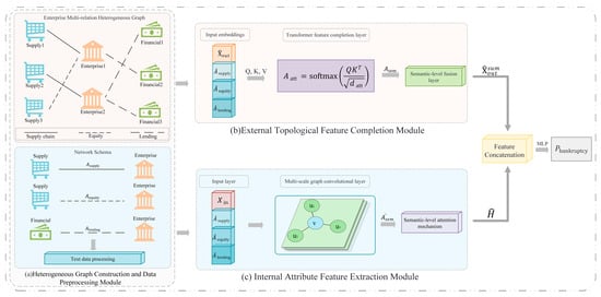
Figure 1.
Model framework diagram.
4.1. Heterogeneous Graph Construction and Data Preprocessing Module
The purpose of this module is to use the multi-relational heterogeneous graph of enterprises as the core data structure, modeling different types of relationships among enterprises to enable more accurate bankruptcy prediction. Specifically, data from enterprises, suppliers, and financial institutions are preprocessed to construct the graph structure based on different network patterns.
As shown in Figure 2a, the enterprise multi-relation heterogeneous graph consists of two key elements: nodes and edges. In the context of this paper, enterprises are the primary nodes, denoted as , where each node represents an enterprise. represents the -th enterprise, and its feature vector includes structured financial data, unstructured information (such as executive backgrounds and enterprise loan records), and other relevant external data that require preprocessing. The supplier node is , where represents the set of all supplier nodes. The feature matrix of the supplier nodes reflects information related to the supply chain categories, cooperation duration, and other relevant relationships with the enterprise. The financial institution node , representing financial institutions that have lending relationships with the enterprise, and the feature matrix describe information related to loans, credit, and other relevant financial aspects.
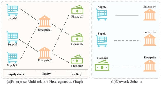
Figure 2.
Enterprise multi-relation heterogeneous graph.
Edges represent relationships between nodes. In this heterogeneous graph, edges have multiple types, each indicating a specific relationship between enterprises and other entities. Supply chain relationships and equity investment relationships exist between enterprises and suppliers, while lending relationships exist between enterprises and financial institutions. Specifically, the supply chain relationship between enterprises and suppliers indicates that suppliers provide raw materials or products to enterprises. The equity investment relationship reflects interactions among shareholders or investors. The lending relationship between enterprises and financial institutions represents loans or financial support provided by institutions to enterprises.
Data preprocessing is the foundation of this module, ensuring that data can effectively apply graph neural networks and accurately reflect complex business relationships and features among enterprises. First, data cleaning is performed to remove redundant or missing enterprise, supplier, and financial institution data. For missing financial or textual data, mean imputation is used to ensure data completeness. Next, structured financial data (such as debt-to-asset ratios and cash flows) undergo feature standardization to eliminate scale differences across features, making them comparable.
For unstructured textual data (such as enterprise loan records and executive backgrounds), the TF-IDF (Term Frequency-Inverse Document Frequency) method is employed for feature extraction. By calculating the term frequency and inverse document frequency of each word, weights are assigned, and the text is converted into numerical vectors. The formulas for TF and IDF are as follows:
Here, is the total number of documents in the collection, and is the number of documents containing the term . Finally, these values are used to generate the feature vector for enterprise data:
In the construction process of a multi-relational heterogeneous graph for enterprises, the textual features of each node are first converted into numerical vectors to form the external initial features of the enterprise, which are then fed as input features into subsequent modules. Next, based on existing business data (such as financial statements, contract records, etc.), relationships between enterprises, suppliers, and financial institutions are labeled to construct corresponding relational adjacency matrices, laying the foundation for graph construction. The specific construction method is as follows: the adjacency matrix represents supply chain relationships, where indicates a supply chain relationship between the -th enterprise and the -th supplier, and indicates no relationship; the adjacency matrix represents lending relationships, where indicates a lending relationship between the -th enterprise and the -th financial institution, and indicates no relationship; the adjacency matrix represents equity investment relationships.
Through these different types of adjacency matrices, this paper constructs a multi-layered graph structure, where each layer reflects a distinct type of relationship, providing a foundation for subsequent module computations. As shown in Figure 2b, the network schema under the multi-relational heterogeneous enterprise graph can be divided into three categories: supply chain relationships, equity investment relationships, and lending relationships. The supply chain relationship schema reflects business collaborations such as raw material procurement, product production, and delivery between enterprises and suppliers. The equity investment relationship schema reflects equity investment or controlling relationships between enterprises and other enterprises. The lending relationship schema reflects fund borrowing relationships between enterprises and financial institutions. The adjacency matrix for each relationship captures specific connections and features between enterprises and their related parties, thereby providing rich relational information for the graph neural network.
These adjacency matrices of different relationships will collectively construct a heterogeneous graph, forming a graph structure that encompasses multiple relationship types, where each relationship type is independently modeled in the graph. Under each network schema, the features of enterprise nodes and related relationships will be aggregated and fused by the external topological feature completion module and the internal attribute feature extraction module to extract deep-level enterprise features. Different relationships (supply chain, equity investment, lending) are modeled through distinct edges in the heterogeneous graph, and ultimately, all features are concatenated and passed to the prediction module.
4.2. External Topological Feature Completion Module
In enterprise bankruptcy prediction, external topological features (supply chain dependencies, industry risks) are crucial for capturing enterprise risks. However, due to data gaps (partial supplier and enterprise information not disclosed), this paper needs to complete these missing features through graph structures and contextual information. The core idea of this module is to fill in these missing data by leveraging the topological relationships between nodes using a Transformer-based attention mechanism approach.
First, for a given multi-relational heterogeneous graph of enterprises. The initial external feature matrix for each enterprise node contains the node’s external information, where is the number of enterprise nodes, and is the external feature dimension. Since some nodes’ external feature matrices have missing values, the missing external features are denoted as , thus obtaining the missing external features , which are completed through the topological relationships between nodes:
Next, the adjacency matrices of the three relationship types need to be mapped to ensure they can be processed in the same dimensional space. Specifically, the adjacency matrices of the three relationship types are as follows: supply chain relationships, equity investment relationships, and lending relationships. To unify the feature space, this paper adopts a linear mapping method, projecting each relationship’s adjacency matrix into the same dimensional space, ensuring these relationships can be uniformly processed in subsequent modules, which are as follows:
: The supply chain relationship matrix, representing the supply chain relationships between enterprises and suppliers.
: The equity investment relationship matrix, representing the equity investment relationships between enterprises and suppliers.
: The lending relationship matrix, representing the lending relationships between enterprises and financial institutions.
Then, for each relationship type’s adjacency matrix, mapping matrices , and are introduced, specifically implemented through the following formula:
Among them, is the original adjacency matrix, representing different types of relationships. is a trainable linear mapping matrix with dimensions , which maps each type of relationship’s adjacency matrix to the same feature space, where is the dimensionality of the mapped feature space. Through this operation, the adjacency matrices of the three different relationships are unified into the same feature space, allowing them to be processed together in subsequent computations.
Next, this module applies the self-attention mechanism of the Transformer to complete the missing external topological features. Here, the query matrix is set as the query vector for each node, the key matrix as the key vector for each node, and the value matrix as the value vector for each node, representing the external feature information of the node. The attention matrix is calculated by the following formula:
Among them, is the attention matrix, representing the association strength between nodes. A weighted average is applied to the attention matrix using the following formula to obtain the completed external feature matrix.
Here, is the completed external feature matrix, representing the result of filling in the missing features.
However, since our enterprise multi-relation heterogeneous graph involves three different relationship patterns (supply chain, equity investment, and lending), the features of the three relationship patterns need to be fused through a semantic-level attention mechanism. Therefore, the feature matrices of the three relationship patterns must first be completed using the above formulas as follows.
Finally, the external features of the three relationships are weighted and fused through the semantic-level attention mechanism to obtain the final external feature embedding. Here, the semantic-level attention matrix is calculated as follows:
Among them, is the learned weight matrix, representing the relative importance of each relationship pattern. The attention matrix is then used to weight and fuse the external features of the three relationships through the following formula, generating the final external feature embedding:
In summary, the external topology feature completion module achieves the completion and information fusion of three enterprise relationship patterns. First, the adjacency matrices of three different relationships are unified into the same feature space through linear mapping. Then, a Transformer-based self-attention mechanism is used to complete missing external features. Finally, a semantic-level attention mechanism is employed to fuse the features of the three relationships, generating comprehensive external feature embeddings. This enables the model to capture complex topological relationships between enterprises, effectively compensating for missing external features and providing more comprehensive input features for enterprise bankruptcy prediction.
4.3. Internal Attribute Feature Extraction Module
Internal attributes of enterprises (such as financial data, cash flow stability, debt-to-asset ratio, etc.) are typically crucial indicators for assessing bankruptcy risk. In this module, this paper employs a multi-layer graph convolutional network (GCN) and a semantic-level attention mechanism to extract and aggregate internal financial features of enterprises. First, this paper aggregates the financial feature information of each node through multi-scale graph convolution, updating the feature representation of each node by aggregating information from neighboring nodes. This captures inter-node relationships and enhances the model’s representational capacity. Specifically, graph convolution aggregates information through a weighted average of the features of a node and its neighboring nodes. Here, the initial feature matrix of enterprise node is , where is the number of enterprise nodes, and is the feature dimension (financial data) of each node.
To effectively extract and fuse internal financial features of enterprises, a multi-layer graph convolutional network (GCN) is used. The multi-scale GCN can capture node information at different levels, thereby enhancing the model’s expressive power. The graph convolution operation at each layer can be updated using the following formula:
Here, is the node feature matrix of the -th layer, representing the aggregated features of the nodes. is the node feature matrix of the -th layer, serving as the input features. is the normalized adjacency matrix, is the graph’s adjacency matrix, and is the degree matrix. is the weight matrix of the -th layer, representing the parameters of each layer. is the activation function , used to increase nonlinear expressive power.
Among them, the normalized adjacency matrix standardizes the original adjacency matrix to ensure that each node can effectively handle the unevenness of node degrees when aggregating neighbor information. Through graph convolution operations, each layer performs information aggregation based on the adjacency relationships of nodes. The more layers there are, the deeper the relationships between nodes the model can capture, and the richer the feature representations of the nodes become.
Secondly, the graph convolution at each layer updates the feature representation of a node by performing a weighted aggregation of its neighboring nodes. For the feature of node at the -th layer, it is obtained through the weighted average of the features of its neighboring nodes, as specified by the following formula:
Here, is the set of neighboring nodes of node , represents the adjacency relationship between node and its neighbor , and is the weight matrix of this layer. Through multi-layer graph convolution operations, this paper can progressively extract deep-level financial information features of enterprise nodes and capture information at different levels.
After multi-layer graph convolution aggregation, the features of enterprise nodes contain aggregated information from various neighbors, but further fusion of these features is still needed to focus on more critical financial characteristics. To achieve this, this paper introduces a semantic-level attention mechanism, which adaptively assigns different weights to each feature, helping the model automatically select the most important features for learning and performing weighted fusion of the aggregated features at each layer. First, the attention weights for the feature matrix of each layer are calculated using the following formula:
Here: is the node feature matrix of the -th layer, representing the aggregated features after multi-layer graph convolution. is the learned semantic-level attention weight matrix, used to compute the weight of each feature. is the attention matrix, representing the weighted relationships between nodes. Through the semantic-level attention mechanism, this paper can generate a weighted feature matrix :
The matrix represents the final fused features, serving as the ultimate feature representation of the nodes, which includes the internal financial risk information of enterprise nodes. In this way, the model can dynamically weight the contributions of different features based on the importance of each node in the graph, ensuring that more critical financial characteristics are assigned higher weights.
This internal attribute feature extraction module aggregates financial data of enterprise nodes through a multi-layer graph convolutional network, progressively extracting deep-level financial features. The internal attribute feature extraction module captures complex interrelationships between enterprise nodes and employs a semantic-level attention mechanism to weight and fuse features from each layer, thereby enhancing the model’s focus on critical internal attributes. Ultimately, the resulting feature representation serves as crucial input for subsequent bankruptcy prediction, aiding the model in better identifying financial risks of enterprises.
In the feature fusion and bankruptcy probability prediction stage, feature fusion is a key step in the enterprise bankruptcy prediction task, integrating information from diverse sources (external and internal) to improve the model’s predictive capability. By combining external features (supply chain, industry risk) and internal features (financial data), a final feature representation encompassing multi-dimensional enterprise information is constructed, and bankruptcy probability is predicted via a multi-layer perceptron (MLP).
First, this paper concatenates the external features and internal features along the feature dimension to obtain a final feature matrix that incorporates both. This is achieved by linking each node’s external and internal feature vectors using the following formula, forming a new feature representation:
Here, denotes the feature concatenation operation. The concatenated feature vector contains all external and internal features of the node, effectively integrating information from two distinct sources. The concatenated feature vector is then fed into a multi-layer perceptron (MLP) for bankruptcy probability prediction. The MLP is a fully connected neural network, typically composed of multiple dense layers and nonlinear activation functions , designed to learn complex mapping relationships between input features and output labels. Finally, the concatenated feature vector is input into the MLP network, which outputs the bankruptcy probability :
Here, represents the multi-layer perceptron (MLP) network, which learns through iterative weighted summation (via weight matrices) of feature vectors and outputs the predicted probability of enterprise bankruptcy. The final output of the MLP is a value between 0 and 1, indicating the likelihood of bankruptcy. During training, the MLP’s parameters are optimized using binary cross-entropy loss, enabling the model to accurately predict enterprise bankruptcy probabilities.
By integrating external features and internal features and inputting them into a MLP, the model can effectively consolidate multi-source enterprise information for accurate bankruptcy probability prediction. As a powerful nonlinear model, the MLP captures complex feature relationships through multi-layer learning and feature transformation, providing reliable support for bankruptcy prediction. Through this module, features from different sources (external and internal) are effectively fused, and bankruptcy probability is predicted via the MLP. This not only enhances feature representation but also captures intricate business relationships through nonlinear mapping.
In summary, the enterprise bankruptcy prediction model proposed in this paper is constructed through three core modules: heterogeneous graph construction and data preprocessing, external topological feature completion, and internal attribute feature extraction. This approach enables the model to effectively integrate financial data, external environmental data, and complex multi-relational networks for precise bankruptcy risk assessment. Ultimately, by concatenating internal and external features and outputting bankruptcy probability through the MLP, the model demonstrates superior performance in handling missing data and complex network structures.
5. Experiments
5.1. Dataset Introduction and Preprocessing
The Industry Financial Overview (IFO) dataset used in this experiment is sourced from Tianyancha (https://www.tianyancha.com/ (accessed on 12 March 2025)) in China, in strict compliance with Tianyancha’s security and privacy policies. It includes large-scale enterprise financial data collected from its online business query platform. The dataset covers 32,459 enterprises (target nodes) from various industries such as manufacturing, financial services, and retail, ensuring the data’s broadness and representativeness. This dataset integrates structured financial information, unstructured textual data, and real-time industry data, providing multi-dimensional support for enterprise bankruptcy risk assessment.
The structured financial data includes core indicators such as the debt-to-asset ratio, operating revenue, cash flow, total assets, and net profit, directly reflecting the enterprise’s ability to repay debt and its operational status. The unstructured textual data consists of information such as litigation records, executive backgrounds, shareholder structures, and related companies, which are transformed into structured vectors using TF-IDF technology to capture potential external factors affecting bankruptcy risk. Real-time industry data includes industry average gross margins and growth rates, helping to analyze the potential impact of the macro-industry environment.
Regarding node features, enterprise nodes have 100-dimensional attributes covering financial indicators, operational indicators, and text mining features; supplier nodes have 24-dimensional attributes, including supply capacity and cooperation history; and financial institution nodes have 56-dimensional attributes, including credit limits and financing costs. The dimensional statistics of the node features are shown in Table 2.
Table 2.
Node Feature Dimension Statistics.
To better model the complex relationships between enterprises, the IFO dataset constructs a multi-relation heterogeneous graph, which includes three types of nodes: enterprise nodes, supplier nodes, and financial institution nodes. It establishes multiple types of edges based on different business relationships, including supply chain relationships, lending relationships, and equity investment relationships. This heterogeneous graph consists of 32,459 nodes and 86,631 edges, with the supply chain edges accounting for the highest proportion. More detailed statistics on nodes and edges are provided in Table 3.
Table 3.
IFO dataset description.
To measure the importance and activity of enterprises in the network, two topological feature indicators are introduced: Quantitative Influence of Relations (QIR) and Transaction Interaction Ratio (TIR).
QIR Definition:
where is the node, is the set of relationship types, and represents the degree of node under relationship type . QIR quantifies the comprehensive connectivity of an enterprise across various relationship types.
TIR Definition:
where represents the weight of the transaction or business relationship between nodes and , and the denominator is the average transaction weight across the entire network. TIR reflects the relative level of enterprise transaction frequency or business interaction within the overall network.
The results in Table 3 show that enterprise nodes generally have higher QIR and TIR values compared to supplier and financial institution nodes, while financial institution nodes are more concentrated in terms of QIR but have larger variations in TIR. This result reveals differences in network structure and business activity among the three types of nodes, providing support for the subsequent model to capture heterogeneous relationships. Additionally, statistical analysis of the weights of different edge relationships (supply chain, lending, and equity) is performed. The results show that the average weight of supply chain edges is the highest, reflecting the stable and frequent transactions between enterprises; lending relationships exhibit greater weight fluctuation, reflecting the diversity and risk uncertainty in financial transactions; and equity relationships show relatively balanced weights, indicating the stability of equity investments between enterprises. These differences in edge weights further reveal the heterogeneity of different edge types in the multi-relation heterogeneous graph, supporting the model in accurately capturing the complex relationships between enterprises.
To ensure label accuracy and temporal independence, this study adopts a prospective labeling strategy. Only data from 1 January 2021 to 1 January 2022 is used as the feature extraction period. Then, using the Tianyancha API, companies that went bankrupt and entered judicial procedures between 1 January 2023 and 31 July 2024 are identified as positive samples (bankrupt), while the remaining companies are labeled as non-bankrupt (negative samples). The bankruptcy status is confirmed based on publicly available legal records from the China Judgments Online (https://wenshu.court.gov.cn/ (accessed on 12 March 2025)) and Tianyancha, ensuring label accuracy and avoiding data leakage. The IFO dataset contains 32,459 companies, of which 1559 (4.8%) went bankrupt after the feature extraction period, reflecting the low-frequency nature of bankruptcy events and highlighting the class imbalance issue. Data is split according to the time-series principle (70%:15%:15%), with the proportion of positive samples in the training, validation, and test sets being 4.7%, 5.1%, and 4.9%, respectively, with a maximum deviation of <0.3%. This ensures that evaluation results are not affected by distribution shifts.
All structured financial data is standardized, and missing values are imputed using the Transformer-based external topology feature completion module. Unstructured text data is converted into structured feature vectors using TF-IDF, and graph data is constructed using multi-relational adjacency matrices to fully capture the diverse relationships between enterprises. Data division strictly follows the temporal sequence, ensuring that only historical data is used during the training and tuning phases to prevent future information leakage.
This study strictly adheres to the relevant laws and regulations of the People’s Republic of China and the security and privacy policies of the Tianyancha platform. The data used are sourced from publicly available and legal channels, solely for academic research purposes, and do not involve any personal privacy information or sensitive data. During data processing, non-essential enterprise information was anonymized and de-identified to ensure data security and compliance. Due to the IFO dataset’s reliance on Tianyancha’s commercial database, it is subject to its terms of use and privacy policies, and the raw data cannot be directly disclosed.
5.2. Baseline Model
This paper compares a total of nine baseline models across three categories, including machine learning (ML) methods, homogeneous graph neural network (HomoG) methods, and heterogeneous graph neural network (HeteG) methods. The details are as follows:
(1) Machine Learning Methods:
1. Logistic Regression [42] (LR): Logistic regression is a classic linear classification method that maps the output of linear regression to a range between 0 and 1 using the Sigmoid function, thereby obtaining the predicted probability of a class. This method is suitable for binary classification problems and can quickly provide linear decision boundaries.
2. Support Vector Machine [12] (SVM): Support vector machine is a widely used supervised learning method for classification and regression problems. Its core idea is to maximize the margin between classes by finding the optimal hyperplane. SVM performs well in high-dimensional feature spaces and can effectively handle nonlinear classification.
3. Decision Tree [43] (DT): Decision tree is a tree-structured classification method that divides samples into different categories through a series of conditional judgments. This method is easy to understand and implement and can handle issues like class imbalance and missing data.
(2) Homogeneous Graph Neural Network Methods:
1. Graph Convolutional Network [44] (GCN): Graph convolutional network (GCN) is one of the classic models in graph deep learning. GCN performs convolutional operations on graphs, propagating feature information from neighboring nodes to the target node, where each node’s features are weighted and aggregated by its neighbors. This enables GCN to effectively capture local structural information among nodes in the graph.
2. Graph Attention Network [45] (GAT): Graph attention network (GAT) introduces a self-attention mechanism based on GCN, automatically computing weights based on the importance of neighboring nodes. During information propagation, each central node aggregates information from its neighbors with adaptive weights, giving the model stronger expressive power, particularly excelling in handling sparse graph data.
(3) Heterogeneous Graph Neural Network Methods:
1. Relational Graph Convolutional Network [39] (RGCN): RGCN is an extension of GCN specifically designed for modeling heterogeneous graphs. By introducing modeling for different types of relationships, RGCN can effectively handle heterogeneous graph data containing multiple types of edges, enhancing the representation capability for complex graph structures.
2. Heterogeneous Graph Attention Network [8] (HAN): HAN employs a hierarchical attention mechanism to perform attention weighting at both the node level and the relationship level, efficiently capturing diverse relational information in heterogeneous graphs. This model initially achieved remarkable results in recommendation systems and has been successfully applied to various domains.
3. Heterogeneous Graph Transformer [40] (HGT): HGT applies the self-attention mechanism from the Transformer to graph neural networks, enabling efficient processing of node and relationship information in heterogeneous graphs. Unlike traditional GCNs, HGT leverages a global attention mechanism to better capture long-range dependencies, improving heterogeneous graph modeling capabilities.
4. Heterogeneous Graph Neural Network Model for Corporate Bankruptcy Prediction [46] (ComRisk): ComRisk utilizes heterogeneous hypergraphs and heterogeneous graphs to model contagion risks among enterprises. By analyzing supply chains, shareholder relationships, and other information, it assesses enterprise bankruptcy risks. This model excels in bankruptcy prediction by comprehensively considering external environments and internal risks.
Through comparisons with these baseline models, the proposed heterogeneous graph neural network-based enterprise bankruptcy prediction model demonstrates superior performance in handling complex relationships and multi-source data. Different types of models help uncover various risk factors, thereby providing more accurate judgment criteria for enterprise bankruptcy prediction.
5.3. Experimental Setup
To comprehensively evaluate the enterprise bankruptcy prediction model proposed in this paper based on heterogeneous graph neural networks (HGNN), six common evaluation metrics were used: accuracy, precision, recall, F1 score, AUC (Area Under the Curve), and AUPRC (Area Under the Precision–Recall Curve). These metrics provide a multi-dimensional assessment of the model’s performance, particularly in addressing the class imbalance issue. AUPRC, in particular, is more effective at reflecting the model’s ability to identify positive class samples.
All experiments were conducted in the same computing environment, with hardware configured as an NVIDIA A100 GPU and an Intel Xeon 32-core processor. For the software environment, the model was implemented using Python 3.8, primarily leveraging the PyTorch 1.12 framework for deep learning model construction and training. The graph neural network portion used the PyTorch Geometric (PyG) 2.1 library to facilitate the construction of heterogeneous graph convolution layers and multi-relation adjacency matrices. The Transformer module relied on PyTorch’s built-in nn.Transformer implementation, combined with a custom multi-head attention mechanism to adapt to the external topology feature completion task. Data preprocessing and feature extraction were performed using the Pandas and Scikit-learn libraries, which included TF-IDF feature extraction and data standardization steps. The following is a detailed configuration and parameter setup for this experiment:
First, the model is trained using the Adam optimizer with an initial learning rate of 0.001. To enhance training stability and avoid gradient explosion or vanishing issues in later stages, a learning rate decay strategy is employed. Specifically, the learning rate decays to 0.9 times its previous value every 10 epochs, aiding the model in gradual convergence during training. For batch training, a batch size of 64 is set to ensure stability, meaning 64 samples are used for each parameter update. This configuration accelerates training while balancing computational efficiency and memory consumption. This model employs a three-layer graph convolutional network (GCN) for feature extraction. Each layer’s graph convolution operation effectively aggregates information from nodes and their neighbors. By stacking multiple convolutional layers, the model captures deep graph structural information while maintaining high computational efficiency.
The specific details of the Transformer design in the external topology feature completion module are as follows:
- ▪
- Number of Layers: A two-layer Transformer encoder is used to balance the model’s expressive power and computational complexity.
- ▪
- Multi-Head Attention: Six attention heads are set, each with a dimension of 128, enhancing the model’s ability to capture relationships between neighboring nodes.
- ▪
- Dropout: A dropout probability of 0.5 is applied to both the attention weights and the feed-forward network output layers to effectively prevent overfitting.
- ▪
- Positional Encoding: The classic sinusoidal positional encoding is used, as defined by the following formulas:
The concatenated feature vector is input into a multi-layer perceptron (MLP) consisting of two fully connected layers. The number of neurons in each layer is 128 and 64, respectively, with the ReLU activation function applied. The output layer uses the Sigmoid function to generate the prediction probability for enterprise bankruptcy. To prevent overfitting during training, L2 regularization is applied with a weight decay coefficient of 0.0005, effectively constraining the model’s complexity and improving its generalization ability. The maximum number of training epochs is set to 50. After each epoch, the model’s performance is evaluated using the validation set, and the best-performing model is saved based on validation performance. These settings ensure the stability of the model across multiple training rounds, achieving high prediction accuracy.
The decision threshold is set by traversing the threshold range [0, 1] in steps of 0.01 on the validation set, calculating the corresponding F1 score for each threshold. The threshold that maximizes the F1 score, 0.48, is selected as the final decision boundary. During the testing phase, this threshold is strictly applied, mapping the predicted probability to class labels to ensure the optimal balance between precision and recall. A strict time-series split is used, dividing the data into training, validation, and test sets with no overlap in the time windows. This prevents any future information leakage. During the testing phase, no adjustments are made to the threshold, ensuring the scientific rigor and fairness of the evaluation.
All hyperparameters and configurations mentioned in this section are detailed in Table 4.
Table 4.
Summary of Key Hyperparameters.
5.4. Comprehensive Model Performance Evaluation
As shown in Table 5, HGNN-EBP outperforms all baseline models across six major evaluation metrics: accuracy, precision, recall, F1 score, AUC, and AUPRC. The model also demonstrates a low standard deviation, reflecting its stability and consistency. Specifically, HGNN-EBP achieves the highest accuracy (0.7633 ± 0.009), precision (0.8136 ± 0.003), recall (0.8156 ± 0.006), F1 score (0.8265 ± 0.003), and AUC (0.8233 ± 0.008), indicating its exceptional performance in enterprise bankruptcy prediction tasks. The small standard deviations further confirm the model’s consistency across multiple experiments, enhancing the reliability of the results.
Table 5.
The overall performance.
In particular, AUPRC, an important metric for addressing class imbalance, better reflects the model’s ability to identify minority class (bankrupt enterprises) samples. HGNN-EBP shows a significant advantage in AUPRC (0.6423 ± 0.006), demonstrating its more stable and superior performance in handling severe class imbalance. Compared to AUC, AUPRC places more emphasis on the balance between precision and recall for the positive class (bankrupt), offering insights into the model’s real-world application capabilities.
To further validate the model’s superiority, Section 5.8 presents parameter analysis that shows performance changes under different hyperparameter configurations, and the introduction of error bars and confidence intervals ensures the stability and scientific rigor of the experimental results. The feature dimension and convolution layer configurations were validated via grid search and 5-fold cross-validation, with statistical reliability ensured through significance testing (t-tests).
Compared to traditional machine learning methods (e.g., LR, SVM, DT) and deep learning models based on homogeneous graph neural networks (GCN, GAT) and heterogeneous graph neural networks (RGCN, HAN, HGT), HGNN-EBP exhibits clear advantages in multi-dimensional data fusion and complex relationship modeling. Traditional methods mainly rely on limited financial features, making it difficult to capture the diverse and complex relationship networks between enterprises, especially when dealing with class imbalance, where performance significantly drops.
GCN has some advantages in feature extraction from graph structures, but it is primarily designed for homogeneous graphs where all nodes and edges are of the same type. In enterprise bankruptcy prediction tasks, however, nodes and edges in the graph vary in type (e.g., firms, suppliers, financial institutions), limiting GCN’s ability to leverage heterogeneous relationship information. GAT introduces an attention mechanism to weigh neighbor node importance but remains confined to homogeneous graphs and may suffer from computational inefficiency when handling large-scale nodes and edges, especially in complex enterprise networks. Although RGCN can process heterogeneous graphs, it has limitations in modeling the depth and granularity of heterogeneous relationships, particularly in capturing dynamic features and higher-order interactions, making it difficult to fully integrate complex information from all node and edge types.
HAN effectively enhances the ability to model heterogeneous relationships through its hierarchical attention mechanism, but its complex structure and computations may lead to performance bottlenecks, especially when processing large-scale data, where computational overhead is significant. HGT incorporates the self-attention mechanism of Transformers, enabling it to capture broader relational information in graph data, yet it still faces challenges in computational efficiency and model training stability, particularly in applications involving large-scale graph structures.
ComRisk, which uses heterogeneous hypergraphs and heterogeneous graphs for enterprise bankruptcy prediction, has achieved some success, with an AUC of 0.8036, but shows shortcomings in balancing precision and recall. Although ComRisk’s accuracy (0.7412 ± 0.000) is close to that of HGNN-EBP, its overall performance does not surpass HGNN-EBP, especially in F1 score and AUC.
HGNN-EBP, by integrating structured financial data, unstructured textual data (such as litigation records and executive backgrounds), and external industry data, is able to consider both internal and external factors in enterprise bankruptcy prediction. This allows the model to explore multi-dimensional potential risk factors in bankruptcy prediction, rather than relying solely on traditional financial data. In contrast, other baseline models (e.g., LR, SVM) focus mainly on structured financial data, neglecting external relationships and unstructured information. The multiple relationships between enterprises (such as supply chains, shareholder relations, and lending) play a critical role in bankruptcy risk. HGNN-EBP, by utilizing heterogeneous graph neural networks (HGNN), constructs a multi-relational graph among enterprises, enabling the model to capture complex relationships between nodes, thereby more accurately modeling bankruptcy risks.
Through multi-scale graph convolution, HGNN-EBP can capture structural information at various levels within the graph, and, with the Transformer attention mechanism, it can effectively handle missing data, ensuring excellent performance even in the presence of incomplete or complex information.
Additionally, to further improve the model’s performance on imbalanced data, the decision threshold was optimized on the validation set, with the threshold (0.48) that maximized the F1 score selected as the final decision boundary. This adjustment improved the balance between precision and recall, enhancing the detection ability of the minority class and contributing to the improvement of AUPRC. During the testing phase, this threshold was strictly applied, and a time-series split was used to ensure that the training, validation, and test sets had no temporal overlap, preventing future information leakage and ensuring fairness and scientific rigor in the evaluation process.
Overall, the success of HGNN-EBP primarily stems from its advantages in multi-source heterogeneous data fusion and heterogeneous graph neural networks. By integrating traditional financial data with complex network relationships, HGNN-EBP can more comprehensively and accurately assess enterprise bankruptcy risks, demonstrating significant superiority over other models across all evaluation metrics. This highlights the strong potential of heterogeneous graph neural networks in the field of enterprise risk assessment and provides robust technical support for future related research.
5.5. ROC Curve Performance Analysis
As shown in Figure 3, the Receiver Operating Characteristic (ROC) curve precisely captures the exceptional discriminative ability of the HGNN-EBP model. The curve presents an ideal convex shape in the false positive rate (FPR) and true positive rate (TPR) coordinate system, with the Area Under the Curve (AUC) reaching 0.8233 (95% confidence interval [0.815, 0.831]), significantly outperforming the random guessing baseline (blue dashed line). The curve’s rapid rise in the low FPR region is particularly striking—when the false positive rate is only 0.015, the true positive rate already reaches 0.8156 (corresponding to a decision threshold of θ = 0.48). This indicates that the model can accurately identify over 81% of bankrupt enterprises while keeping the misclassification rate below 1.5%, showcasing excellent early risk warning capability.
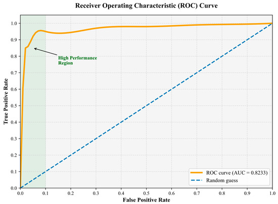
Figure 3.
Receiver Operating Characteristic curve.
The shallow, green high-performance region labeled in the upper left of the curve highlights a steep upward slope, which intuitively reflects the model’s precise discriminatory ability achieved through multi-source data fusion, including structured financial data, unstructured textual information, and complex relational networks. Notably, within the range of FPR ∈ [0.02, 0.05], the curve exhibits an almost linear upward trend, revealing the heterogeneous graph neural network’s strong capability in capturing complex relational features, such as those from supply chains and lending relationships.
The narrow 95% confidence interval further validates the stability of the model’s performance. Statistical tests confirm that the AUC value significantly outperforms the best baseline, ComRisk (ΔAUC = 0.0197, t = 5.13, p = 0.0004). The overall shape of the curve, together with the high AUPRC value (0.6423) reported in Table 5, mutually corroborates the model’s robustness in handling severely imbalanced class scenarios, where bankrupt enterprises account for only 4.8% of the total data. This high recall feature with a low false positive rate enhances the practical application value of HGNN-EBP in real-world financial risk control systems.
5.6. Node Clustering Experiment
To validate the effectiveness of the proposed HGNN-EBP model, this paper conducted node clustering experiments to evaluate the performance of different graph neural network (GNN) models in node representation learning. As shown in Table 6, in the clustering experiments, this paper first obtained the embeddings of enterprise nodes through the forward propagation of each GNN model, then applied the K-Means algorithm for node clustering, and finally used two metrics—Normalized Mutual Information (NMI) and Adjusted Rand Index (ARI)—to assess the quality of clustering results from the perspectives of consistency and accuracy, respectively. NMI measures the similarity between predicted clusters and true labels, while ARI evaluates the accuracy of clustering results by accounting for the impact of randomness.
Table 6.
Node clustering experimental results.
The experimental results in the table demonstrate that HGNN-EBP performs exceptionally well on both ARI (Adjusted Rand Index) and NMI (Normalized Mutual Information) metrics, significantly outperforming other models. Specifically, HGNN-EBP achieves an ARI of 0.2589 and an NMI of 0.2149, whereas the results of other models are generally lower. For example, GCN yields an ARI of 0.0263 and an NMI of 0.0741, while GAT even produces a negative ARI value (−0.0214), indicating poor performance in the node clustering task. A higher ARI value reflects stronger alignment between clustering results and true labels. HGNN-EBP excels in this metric, significantly surpassing GCN (0.0263), GAT (−0.0214), and RGCN (−0.0099). By fusing structured financial data, unstructured textual data, and external topological relationships, HGNN-EBP captures the complex inter-enterprise relationships, better revealing latent classifications and leading to higher ARI values.
Other models, such as GCN and GAT, struggle to capture the intricate relational structures among corporations due to their inability to model heterogeneous graphs, resulting in lower accuracy of clustering outcomes and consequently lower or even negative ARI values.
A higher NMI value indicates that the clustering results of the model better reflect the distribution of true labels. The NMI of HGNN-EBP is 0.2149, significantly higher than other models (e.g., 0.0369 for GAT and 0.0741 for GCN). This demonstrates that HGNN-EBP can generate more accurate node representations, enabling the K-Means algorithm to better capture the intrinsic structure of the data during clustering. In contrast, the lower NMI values of GCN and GAT suggest that their node representations in clustering tasks are relatively ambiguous, failing to effectively distinguish the latent differences between enterprise nodes.
The advantages of HGNN-EBP over other baseline models in node clustering experiments are mainly reflected in the following aspects: HGNN-EBP effectively models the diverse relationships between enterprises (such as supply chains, shareholders, and lending relationships) through heterogeneous graph neural networks, resulting in more accurate and comprehensive representations of enterprise nodes. In contrast, traditional GCN and GAT models fail to account for heterogeneous relationships, leading to poorer clustering results. HGNN-EBP employs a Transformer attention mechanism to complete missing external features, making the model more robust when facing incomplete data. This characteristic allows HGNN-EBP to maintain high clustering performance in practical applications, especially in scenarios with incomplete data.
5.7. Ablation Study
From the ablation study results in Table 7, it can be observed that HGNN-EBP significantly outperforms other variants across all evaluation metrics (accuracy, precision, recall, F1 score, and AUC). Specifically, HGNN-EBP achieves an accuracy of 0.7633 ± 0.009, precision of 0.8136 ± 0.003, recall of 0.8156 ± 0.006, F1 score of 0.8265 ± 0.003, and AUC of 0.8233 ± 0.003. In comparison with versions where certain modules are removed, HGNN-EBP still demonstrates markedly superior performance, highlighting the critical contributions of each module to the model’s overall performance. Among these are the following:
w/o-HeteG: Removing the heterogeneous graph modeling module.
w/o-Trans: Removing the Transformer attention mechanism.
w/o-Inter: Removing the internal attribute feature extraction module.
Table 7.
Ablation experiment results.
Table 7.
Ablation experiment results.
| Models | Accuracy | Precision | Recall | F1 score | AUC |
|---|---|---|---|---|---|
| HGNN-EBP | 0.7633 ± 0.009 | 0.8136 ± 0.003 | 0.8156 ± 0.006 | 0.8265 ± 0.003 | 0.8233 ± 0.001 |
| w/o-HeteG | 0.5416 ± 0.008 | 0.6523 ± 0.003 | 0.9233 ± 0.006 | 0.5912 ± 0.001 | 0.2369 ± 0.002 |
| w/o-Trans | 0.6523 ± 0.007 | 0.6955 ± 0.002 | 0.8562 ± 0.006 | 0.8001 ± 0.001 | 0.3259 ± 0.003 |
| w/o-Inter | 0.7044 ± 0.009 | 0.7539 ± 0.002 | 0.8437 ± 0.005 | 0.7439 ± 0.002 | 0.5172 ± 0.002 |
After removing the heterogeneous graph modeling (HeteG) module, the model’s performance significantly declined, with accuracy dropping to 0.5416 ± 0.008, precision to 0.6523 ± 0.003, F1 score to 0.5912 ± 0.001, and AUC to only 0.2369 ± 0.002. The notable drop in the AUC metric indicates that without heterogeneous graph modeling, the model lost its ability to capture complex relationships between different types of nodes, leading to a substantial reduction in the discriminative power and accuracy of predictions. This demonstrates the critical role of the heterogeneous graph modeling module in fully characterizing the diverse relationships among enterprises and improving prediction accuracy. The results further suggest that a single homogeneous graph network (e.g., GCN) cannot effectively capture the varied interactions and dependencies among enterprises, resulting in a significant decline in clustering and prediction performance. After removing the Transformer attention mechanism, the model’s accuracy was 0.6523 ± 0.007, precision 0.6955 ± 0.002, recall 0.8562 ± 0.006, F1 score 0.8001 ± 0.001, while AUC dropped to 0.3259 ± 0.003. Although the recall remained relatively high (0.8562) without the Transformer attention mechanism, indicating the model could still capture a certain number of positive samples, the significant declines in AUC and F1 score suggest reduced predictive discriminability and a potential increase in false positives. This proves the importance of the Transformer self-attention mechanism in the external feature completion module, effectively addressing feature missing issues and enhancing the model’s robustness in handling complex relationships.
After removing the internal attribute feature extraction module (Inter), the model’s accuracy was 0.7044 ± 0.009, precision 0.7539 ± 0.002, recall 0.8437 ± 0.005, F1 score 0.7439 ± 0.002, and AUC 0.5172 ± 0.002. Although the recall was high, the lower accuracy and AUC indicate that without the internal feature extraction module, the model failed to effectively extract and integrate internal information such as financial data, leading to performance degradation. This suggests that graph convolution operations are crucial for deeply mining relationships between nodes and feature aggregation, particularly in enterprise bankruptcy prediction, where combining internal and external data can significantly enhance the model’s overall performance.
Through ablation experiments, this paper can clearly observe the contributions of each module to the HGNN-EBP model. The heterogeneous graph modeling module, Transformer attention mechanism, and internal attribute feature extraction module played vital roles in improving model performance. Notably, the heterogeneous graph modeling module significantly enhanced prediction accuracy and discriminability, while the Transformer attention mechanism improved the ability to handle missing data. The internal feature extraction module effectively integrated financial data and external relationship information through graph convolution layers, further strengthening the model’s comprehensive predictive capability.
5.8. Parameter Analysis
To further enhance the performance of the HGNN-EBP model, this paper conducts a systematic analysis of two critical hyperparameters: the feature dimension in the Transformer attention mechanism of the external topology feature completion module and the number of convolution layers in the internal attribute feature extraction module. These two hyperparameters play a crucial role in model training, feature learning, and overall performance. The experimental results are shown in Figure 4 and Figure 5.
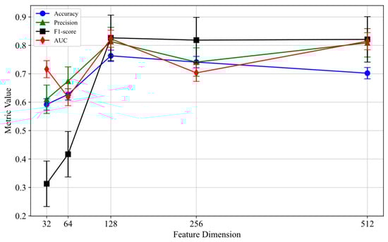
Figure 4.
Feature dimension analysis.
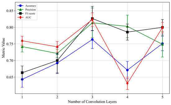
Figure 5.
Convolutional layer count analysis.
Feature Dimension Analysis: As shown in Figure 4, this study systematically evaluates the impact of different feature dimensions on model performance. In the feature dimension analysis, the number of convolution layers is fixed at three to ensure that the evaluation results are solely influenced by the feature dimension changes. As the feature dimension increases from 32 to 128, the model’s accuracy improves significantly from 0.59 ± 0.01 to 0.76 ± 0.01, and the F1 score jumps from 0.31 ± 0.03 to 0.83 ± 0.03. This indicates that the 128-dimensional feature strikes an optimal balance between representational capability and computational efficiency. Notably, when the dimension extends to 256 or 512, a clear overfitting phenomenon occurs: the precision drops from its peak of 0.81 ± 0.02 to 0.10 ± 0.04, and the 95% confidence interval expands 3-fold (from ±0.012 to ±0.038). This conclusion is rigorously validated through grid search (search space: {32, 64, 128, 256, 512}, 5-fold cross-validation). The error bars in these experimental results represent the standard error for each hyperparameter setting, showing the significant impact of feature dimension changes on model performance.
Convolution Layer Number Analysis: As shown in Figure 5, this paper evaluates the impact of different convolution layer numbers on model performance, keeping the feature dimension fixed at 128 to ensure that the results are influenced only by the convolution layer count. The results indicate that the performance is optimal with three convolution layers, where the accuracy is 0.76 ± 0.02, the F1 score is 0.83 ± 0.07, and the AUC is 0.82 ± 0.03. Three convolution layers effectively capture deep relationships between nodes, while fewer (e.g., one layer) or more (e.g., four or five layers) layers lead to performance degradation. The error bars in Figure 5 show the variability of different convolution layer configurations. Grid search confirms that three layers are the optimal configuration. Figure 5 also reveals the nonlinear effect of the number of convolution layers, where the three-layer architecture achieves the best balance across all metrics, significantly outperforming other configurations (see Table 8). Specifically, the one- to two-layer configurations suffer an 18% reduction in AUC due to insufficient representational power (0.65 ± 0.03 vs. 0.82 ± 0.03, p < 0.001); when the number of layers reaches four or more, the gradient vanishing issue increases the variance of the F1 score by 300% (from 0.002 to 0.006). Additionally, statistical tests show that the performance difference between three layers and four layers is highly significant (accuracy: p = 0.0001, effect size d = 1.32), and this advantage remains stable at a 95% confidence interval.
Table 8.
Convolution layer number significance test.
Statistical Significance Test: To verify the significance of the 3-layer convolution configuration, this study conducted statistical significance tests (t-test) on different convolution layer counts. Table 8 shows the t-test results comparing convolution layers, where p-values for comparisons such as 1-layer vs. 3-layer, 2-layer vs. 3-layer, and 3-layer vs. 4-layer are all less than 0.05, indicating statistical significance. The 3-layer convolution stands out across various performance metrics (accuracy, precision, F1 score, and AUC).
The t-test results show that the comparisons between 1-layer vs. 3-layer, 2-layer vs. 3-layer, and 3-layer vs. 4-layer, among others, have p-values less than 0.05, indicating statistical significance. Particularly, the 3-layer convolution configuration stands out in various performance metrics (accuracy, precision, F1 score, and AUC). Based on the experimental results and statistical analysis, we select 128-dimensional features and three convolution layers as the optimal configuration for the HGNN-EBP model. This configuration effectively improves model performance and demonstrates good robustness. By incorporating error bars and grid search validation, this study further enhances the reliability and scientific basis for the selection of model configurations.
5.9. Quantitative Validation of the External Topological Feature Completion Module for Missing Values
In terms of missing value handling, this paper first calculates the missing ratios and missing patterns (MCAR, MAR, MNAR) for each relationship type in the dataset. The results show that the overall missing ratio for structured financial indicators is 7.3%, with the missing rates for operating income and cash flow being relatively higher. The missing ratio for unstructured text features (e.g., executive background) is 4.6%, and the missing ratio for external industry data is less than 2%. Missing pattern analysis indicates that most of the missing data falls under Missing At Random (MAR), which is primarily related to company size and industry category.
To validate the effectiveness of the external topological feature completion module (ETFCM), this study designed and conducted a systematic quantitative evaluation experiment, focusing on testing the module’s performance under various missing rates and missing patterns. Considering the complexity of missing data in real-world enterprise datasets, two common missing patterns were simulated: Missing Completely At Random (MCAR) and Missing At Random (MAR). MCAR indicates that the missing values are randomly distributed and independent of the data itself, while MAR suggests that the missing values depend on observable other variables but not on the missing value itself. Since Missing Not At Random (MNAR) presents higher modeling complexity and requires special treatment, it was not included in this experiment; this will be explored in future studies.
The experiment was conducted based on the initial external topological feature matrix , where feature values were randomly masked at three rates, 10%, 20%, 30%, to simulate MCAR and MAR missing patterns, forming test sets with missing values. The proposed external topological feature completion module, based on the Transformer self-attention mechanism, was used to predict and fill the missing values. For a fair comparison, two classical imputation methods, K-Nearest Neighbors (KNN) and Multiple Imputation by Chained Equations (MICE), were chosen as baselines.
The evaluation metrics used were Root Mean Squared Error (RMSE) and Mean Absolute Error (MAE), which measure the error size between the imputed results and the real complete data. Table 9 shows the RMSE and MAE comparison results of the proposed method and baseline methods under different missing rates and missing patterns. The experimental results indicate that regardless of the missing rate or whether the MCAR or MAR missing pattern is applied, the proposed Transformer-based imputation module consistently outperforms KNN and MICE methods, demonstrating lower RMSE and MAE. This confirms the module’s ability to utilize multi-relational heterogeneous graph topology and complex semantic relationships between nodes, significantly improving the accuracy of missing data imputation.
Table 9.
Performance comparison of the external topological feature completion module for missing value imputation.
In conclusion, this experiment systematically validated the superior performance of the Transformer-based external topological feature completion module in the missing value imputation task. This enhances the input data quality for the bankruptcy prediction model and provides solid theoretical and empirical support for graph-based and deep learning-based missing data imputation methods.
6. Discussion
This study proposes a bankruptcy prediction model based on heterogeneous graph neural networks (HGNN-EBP), which integrates both internal and external features of enterprises to deeply explore bankruptcy risks. Building on traditional methods that rely on structured financial data, this research successfully addresses the limitations of conventional models by introducing HGNN, which considers the complex, multi-layered relationships between enterprises and external environmental factors. The following outlines the contributions and innovations of this study compared to the existing literature.
Traditional bankruptcy prediction methods, such as logistic regression and decision trees, mainly rely on structured financial data and often fail to capture the complex relational networks between enterprises. Although there have been attempts in recent years to apply graph neural networks (GNNs) to bankruptcy prediction, most of these have been limited to homogeneous GNNs, without fully leveraging the heterogeneous relationships between enterprises. This study overcomes this limitation by constructing a multi-relational heterogeneous graph, which comprehensively considers various relationships such as supply chains, shareholder investments, and lending, significantly improving bankruptcy prediction accuracy. The existing literature indicates that heterogeneous GNNs perform well in multiple fields, yet their application in bankruptcy prediction remains limited. The innovation of this study lies in the successful application of HGNNs in this domain, where multi-scale graph convolutional networks enhance the model’s ability to capture relationships at different levels. Experimental results demonstrate that the model can effectively capture the complex, multi-layered heterogeneous relationships between enterprises, improving the robustness of bankruptcy predictions.
In bankruptcy prediction, missing data is a common problem, particularly the absence of external topology features (e.g., supplier relationships). Traditional imputation methods such as KNN cannot effectively handle these complex relational data. To address this, this study proposes a dynamic imputation method based on a Transformer self-attention mechanism, significantly improving the accuracy of imputed data and the model’s predictive capability. The issue of class imbalance in bankruptcy prediction has been a longstanding challenge. In this study, the model’s decision threshold was optimized to maximize the F1 score, improving its ability to predict minority class (bankrupt enterprises). Experimental results show that the model performs excellently in cases of class imbalance, with a high AUPRC value, further demonstrating its potential for application in practical financial risk management.
By introducing heterogeneous graph neural networks and Transformer mechanisms, this study proposes an innovative bankruptcy prediction method that successfully integrates structured financial data, unstructured text data, and complex relational information between enterprises. Compared to traditional methods, HGNN-EBP captures bankruptcy risks more comprehensively and accurately, especially excelling in handling class imbalance and missing data. Future research can further optimize and extend this model to improve its application performance in dynamic and complex environments.
7. Conclusions
This paper proposes a bankruptcy prediction algorithm based on heterogeneous graph neural networks (HGNNs) and the integration of external features and internal attributes—HGNN-EBP. The goal is to enhance the accuracy, robustness, and adaptability of enterprise bankruptcy prediction by integrating multi-source heterogeneous data, including structured financial data, unstructured textual information, and external industry data. The experimental results show that HGNN-EBP outperforms other models across several evaluation metrics, including accuracy, precision, recall, F1 score, and AUC, with particular advantages in handling the complex multi-relational network among enterprises.
Ablation experiments further reveal the importance of key modules, such as the heterogeneous graph modeling module and the internal attribute feature extraction module, in improving model performance. Specifically, the graph convolution-based feature extraction module effectively captures the multi-layered relationships among enterprises, and the Transformer attention mechanism, which handles missing data, further enhances the model’s robustness to incomplete information. The experiments also demonstrate that appropriately selecting feature dimensions and convolution layers significantly improves the model’s generalization ability, preventing overfitting and excessive computational complexity, thus ensuring the model’s efficiency in real-world applications.
Moreover, the proposed HGNN-EBP not only predicts based on traditional financial data but also provides a more comprehensive risk assessment by incorporating external relational data through an innovative graph neural network architecture. This breaks the dependence of traditional prediction models on a single data source and provides a powerful tool for risk assessment in the financial sector.
However, this study does have some limitations. First, although the model incorporates multiple data sources (e.g., financial data, industry data, and textual information), data quality and completeness remain a challenge during the preprocessing phase. For instance, missing or incomplete unstructured data for some enterprises may impact the model’s final performance. Second, while the model demonstrates strong robustness, its effectiveness in handling extreme situations, such as bankruptcy prediction during economic crises or in specific industry environments, still requires further validation. Additionally, the model is computationally expensive in terms of resource consumption and training time, posing challenges for application on large-scale datasets.
Future research will explore combining federated learning mechanisms to enable the enterprise bankruptcy prediction model to perform collaborative modeling across institutions while completing training without sharing sensitive data. The introduction of federated learning will not only protect data privacy effectively but also enable cross-institutional data sharing and knowledge dissemination, enhancing the model’s universality, robustness, and adaptability. Additionally, future studies will further investigate how to improve the model’s predictive ability for abnormal enterprises and extreme situations, such as bankruptcy risk assessment during economic crises or within special industry environments, thereby improving its adaptability and reliability for broader applications in complex financial market settings.
In conclusion, HGNN-EBP, as an enterprise bankruptcy prediction model integrating multi-source data with heterogeneous graph neural networks, offers high prediction accuracy and practical value. Through multi-dimensional data fusion and fine-grained modeling, this model provides a more accurate and comprehensive enterprise risk assessment for the financial sector, driving further development in the field.
Author Contributions
Conceptualization, X.D. and J.D.; Methodology, X.D. and Z.T.; Software, J.C. and X.W.; Validation, J.C.; Formal analysis, X.J.; Investigation, X.J.; Resources, J.D.; Data curation, J.D. and Z.T.; Writing—original draft, X.D.; Writing—review & editing, J.D.; Visualization, X.W.; Supervision, J.C.; Project administration, J.C. and X.W.; Funding acquisition, J.C. All authors have read and agreed to the published version of the manuscript.
Funding
This research was funded by the Jiangsu Science and Technology Think Tank Program (Youth Project) grant number JSKX24091, and the Jiangsu Provincial University Philosophy and Social Science Research General Project grant number 2024SJYB1077. The APC was funded by the authors.
Data Availability Statement
The data presented in this study are available on request from the corresponding author.
Conflicts of Interest
Author Xiong Wang was employed by the company Celanese (China) Holding Co., Ltd. Nanjing. The authors declare no conflict of interest.
References
- Altman, E.I.; Iwanicz-Drozdowska, M.; Laitinen, E.K.; Suvas, A. Financial distress pediction in an international context: A review and empirical analysis of Altman’s Z-score model. J. Int. Financ. Manag. Account. 2017, 28, 131–171. [Google Scholar] [CrossRef]
- Altman, E.I.; Iwanicz-Drozdowska, M.; Laitinen, E.K.; Suvas, A. Distressed Firm and Bankruptcy Prediction in an International Context: A Review and Empirical Analysis of Altman’s Z-Score Model. 2014. Available online: https://ssrn.com/abstract=2536340 (accessed on 22 June 2025).
- Almamy, J.; Aston, J.; Ngwa, L.N. An evaluation of Altman’s Z-score using cash flow ratio to predict corporate failure amid the recent financial crisis: Evidence from the UK. J. Corp. Financ. 2016, 36, 278–285. [Google Scholar] [CrossRef]
- Xu, C.; Huang, H.; Ying, X.; Gao, J.; Li, Z.; Zhang, P.; Xiao, J.; Zhang, J.; Luo, J.J. HGNN: Hierarchical graph neural network for predicting the classification of price-limit-hitting stocks. Inf. Sci. 2022, 607, 783–798. [Google Scholar] [CrossRef]
- Zhao, Z.; Liu, Z.; Wang, Y.; Yang, D.; Che, W. RA-HGNN: Attribute completion of heterogeneous graph neural networks based on residual attention mechanism. Expert Syst. Appl. 2024, 243, 122945. [Google Scholar] [CrossRef]
- Fu, X.; Li, J.; Wu, J.; Sun, Q.; Ji, C.; Wang, S.; Tan, J.; Peng, H.; Yu, P.S. ACE-HGNN: Adaptive curvature exploration hyperbolic graph neural network. In Proceedings of the 2021 IEEE International Conference on Data Mining (ICDM), Auckland, New Zealand, 7–10 December 2021; pp. 111–120. [Google Scholar]
- Chen, T.; Guestrin, C. Xgboost: A scalable tree boosting system. In Proceedings of the 22nd ACM SIGKDD International Conference on Knowledge Discovery and Data Mining, San Francisco, CA, USA, 13–17 August 2016; pp. 785–794. [Google Scholar]
- Wang, X.; Ji, H.; Shi, C.; Wang, B.; Ye, Y.; Cui, P.; Yu, P.S. Heterogeneous graph attention network. In Proceedings of the World Wide Web Conference, San Francisco, CA, USA, 13–17 May 2019; pp. 2022–2032. [Google Scholar]
- Chung, K.C.; Tan, S.S.; Holdsworth, D.K. management. Insolvency prediction model using multivariate discriminant analysis and artificial neural network for the finance industry in New Zealand. Int. J. Bus. Manag. 2008, 39, 19–28. [Google Scholar]
- Lee, S.; Choi, W.S. A multi-industry bankruptcy prediction model using back-propagation neural network and multivariate discriminant analysis. Expert Syst. Appl. 2013, 40, 2941–2946. [Google Scholar] [CrossRef]
- Peres, C.; Antão, M. The use of multivariate discriminant analysis to predict corporate bankruptcy: A review. AESTIMATIO IEB Int. J. Financ. 2017, 14, 108–131. [Google Scholar]
- Jakkula, V. Tutorial on Support Vector Machine (SVM); School of EECS, Washington State University: Pullman, WA, USA, 2006; Volume 37, p. 3. [Google Scholar]
- De Ville, B. Decision trees. WIREs Comput. Stat. 2013, 5, 448–455. [Google Scholar] [CrossRef]
- Roesel, K.; Dohoo, I.; Baumann, M.; Dione, M.; Grace, D.; Clausen, P.-H. Prevalence and risk factors for gastrointestinal parasites in small-scale pig enterprises in Central and Eastern Uganda. Parasitol. Res. 2017, 116, 335–345. [Google Scholar] [CrossRef]
- Ming, W.; Xiao, X.; Tian, L.; Shen, N. Risk Contagion Effects of Interconnected Manufacturing Enterprises. IgMin Res. 2024, 2, 759–767. [Google Scholar] [CrossRef]
- Wang, W.; Tang, D.; Xu, R. Systemic risk infection and control of water eco-environmental projects under the mode of government-enterprise cooperation. J. Coast. Res. 2020, 103, 447–452. [Google Scholar] [CrossRef]
- Hu, Z.; Dong, Y.; Wang, K.; Chang, K.-W.; Sun, Y. Gpt-gnn: Generative pre-training of graph neural networks. In Proceedings of the 26th ACM SIGKDD International Conference on Knowledge Discovery & Data Mining, Virtual Event, 6–10 July 2020; pp. 1857–1867. [Google Scholar]
- Wu, L.; Chen, Y.; Shen, K.; Guo, X.; Gao, H.; Li, S.; Pei, J.; Long, B. Graph Neural Networks for Natural Language Processing: A Survey; Now Foundations and Trends: Norwell, MA, USA, 2023; Volume 16, pp. 119–328. [Google Scholar]
- Wu, S.; Sun, F.; Zhang, W.; Xie, X.; Cui, B. Graph neural networks in recommender systems: A survey. ACM Comput. Surv. 2022, 55, 1–37. [Google Scholar] [CrossRef]
- Pradhyumna, P.; Shreya, G. Graph neural network (GNN) in image and video understanding using deep learning for computer vision applications. In Proceedings of the 2021 Second International Conference on Electronics and Sustainable Communication Systems (ICESC), Coimbatore, India, 4–6 August 2021; pp. 1183–1189. [Google Scholar]
- Cheng, D.; Zou, Y.; Xiang, S.; Jiang, C. Graph neural networks for financial fraud detection: A review. Front. Comput. Sci. 2025, 19, 199609. [Google Scholar] [CrossRef]
- Zhang, X.; Xu, Z.; Liu, Y.; Sun, M.; Zhou, T.; Sun, W. Robust Graph Neural Networks for Stability Analysis in Dynamic Networks. In Proceedings of the 2024 3rd International Conference on Cloud Computing, Big Data Application and Software Engineering (CBASE), Hangzhou, China, 11–13 October 2024; pp. 806–811. [Google Scholar]
- Kesharwani, A.; Shukla, P. FFDM−GNN: A Financial Fraud Detection Model using Graph Neural Network. In Proceedings of the 2024 International Conference on Computing, Sciences and Communications (ICCSC), Ghaziabad, India, 24–25 October 2024; pp. 1–6. [Google Scholar]
- Zhao, Z.; Qian, P.; Yang, X.; Zeng, Z.; Guan, C.; Tam, W.L.; Li, X. Semignn-ppi: Self-ensembling multi-graph neural network for efficient and generalizable protein-protein interaction prediction. In Proceedings of the Thirty-Second International Joint Conference on Artificial Intelligence, Macao, China, 19–25 August 2023. [Google Scholar]
- Pu, Y.; Chen, Y.; Fan, J. P2P Lending Default Risk Prediction Using Attention-Enhanced Graph Neural Networks. Adv. Comput. Syst. 2023, 3, 8–20. [Google Scholar] [CrossRef]
- Cheng, D.; Niu, Z.; Li, J.; Jiang, C. Regulating systemic crises: Stemming the contagion risk in networked-loans through deep graph learning. IEEE Trans. Knowl. Data Eng. 2022, 35, 6278–6289. [Google Scholar] [CrossRef]
- Wasi, A.T.; Islam, M.; Akib, A.R. Supplygraph: A benchmark dataset for supply chain planning using graph neural networks. arXiv 2024, arXiv:2401.15299. [Google Scholar] [CrossRef]
- Huang, K.; Li, X.; Liu, F.; Yang, X.; Yu, W. ML-GAT: A multilevel graph attention model for stock prediction. IEEE Access 2022, 10, 86408–86422. [Google Scholar] [CrossRef]
- Bi, W.; Xu, B.; Sun, X.; Wang, Z.; Shen, H.; Cheng, X. Company-as-tribe: Company financial risk assessment on tribe-style graph with hierarchical graph neural networks. In Proceedings of the 28th ACM SIGKDD Conference on Knowledge Discovery and Data Mining, Washington, DC, USA, 14–18 August 2022; pp. 2712–2720. [Google Scholar]
- Zhao, X.; Wu, J.; Peng, H.; Beheshti, A.; Monaghan, J.J.; McAlpine, D.; Hernandez-Perez, H.; Dras, M.; Dai, Q.; Li, Y. Deep reinforcement learning guided graph neural networks for brain network analysis. Neural Netw. 2022, 154, 56–67. [Google Scholar] [CrossRef]
- Gava, R.; Zulauf, U. Enforcement of Financial Regulation in Switzerland: A New Dataset and Empirical Overview of FINMA Enforcement. 2025. Available online: https://ssrn.com/abstract=5327371 (accessed on 24 June 2025).
- Dlamini, T.; Khumalo, N.; Mthembu, K.; Mokoena, A. Research on a multimodal stock trend prediction model integrating image generation and financial text analysis. Comput. Educ. Lett. 2025, 2, 1–8. [Google Scholar]
- Wan, Q.; Wan, C.; Hu, R.; Liu, D.; Xu, W.; Xu, K.; Zou, M.; Tao, L.; Yang, J.; Xiong, Z. OEE-CFC: A Dataset for Open Event Extraction from Chinese Financial Commentary. In Findings of the Association for Computational Linguistics: EMNLP 2024; Association for Computational Linguistics: Miami, FL, USA, 2024; pp. 4446–4459. [Google Scholar]
- Jiang, Y.; Ning, K.; Pan, Z.; Shen, X.; Ni, J.; Yu, W.; Schneider, A.; Chen, H.; Nevmyvaka, Y.; Song, D. Multi-modal time series analysis: A tutorial and survey. In Proceedings of the 31st ACM SIGKDD Conference on Knowledge Discovery and Data Mining, Toronto, ON, Canada, 3–7 August 2025; Volume 2, pp. 6043–6053. [Google Scholar]
- Wang, J.; Liu, X.; Li, W.; Liu, F.; Wu, X.; Jin, Q. A text-enhanced transformer fusion network for multimodal knowledge graph completion. IEEE Intell. Syst. 2024, 39, 54–62. [Google Scholar] [CrossRef]
- He, L.; Bai, L.; Yang, X.; Du, H.; Liang, J. High-order graph attention network. Inf. Sci. 2023, 630, 222–234. [Google Scholar] [CrossRef]
- Shumovskaia, V.; Fedyanin, K.; Sukharev, I.; Berestnev, D.; Panov, M. Linking bank clients using graph neural networks powered by rich transactional data. Int. J. Data Sci. Anal. 2021, 12, 135–145. [Google Scholar] [CrossRef]
- Zeng, Y.; Jin, Q.; Bao, T.; Li, W. Multi-modal knowledge hypergraph for diverse image retrieval. In Proceedings of the AAAI Conference on Artificial Intelligence, Washington, DC, USA, 7–14 February 2023; pp. 3376–3383. [Google Scholar]
- Chen, J.; Hou, H.; Gao, J.; Ji, Y.; Bai, T. RGCN: Recurrent graph convolutional networks for target-dependent sentiment analysis. In Proceedings of the International Conference on Knowledge Science, Engineering and Management, Athens, Greece, 28–30 August 2019; pp. 667–675. [Google Scholar]
- Hu, Z.; Dong, Y.; Wang, K.; Sun, Y. Heterogeneous graph transformer. In Proceedings of the Web Conference 2020, Taipei, Taiwan, 20–24 April 2020; pp. 2704–2710. [Google Scholar]
- Bi, W.; Du, L.; Fu, Q.; Wang, Y.; Han, S.; Zhang, D. Mm-gnn: Mix-moment graph neural network towards modeling neighborhood feature distribution. In Proceedings of the Sixteenth ACM International Conference on Web Search and Data Mining, Singapore, 27 February–3 March 2023; pp. 132–140. [Google Scholar]
- LaValley, M.P. Logistic regression. Circulation 2008, 117, 2395–2399. [Google Scholar] [CrossRef] [PubMed]
- Quinlan, J.R. Learning decision tree classifiers. ACM Comput. Surv. 1996, 28, 71–72. [Google Scholar] [CrossRef]
- Zhang, S.; Tong, H.; Xu, J.; Maciejewski, R. Graph convolutional networks: A comprehensive review. Comput. Soc. Netw. 2019, 6, 11. [Google Scholar] [CrossRef] [PubMed]
- Veličković, P.; Cucurull, G.; Casanova, A.; Romero, A.; Lio, P.; Bengio, Y. Graph attention networks. arXiv 2017, arXiv:1710.10903. [Google Scholar]
- Andersson, M.G.; Elving, J.; Nordkvist, E.; Urdl, M.; Engblom, L.; Mader, A.; Altmeyer, S.; Kowalczyk, J.; Lahrssen-Wiederholt, M.; Tuominen, P. Communication inside Risk Assessment and Risk Management (COMRISK). EFSA Support. Publ. 2020, 17, 1891E. [Google Scholar] [CrossRef]


Disclaimer/Publisher’s Note: The statements, opinions and data contained in all publications are solely those of the individual author(s) and contributor(s) and not of MDPI and/or the editor(s). MDPI and/or the editor(s) disclaim responsibility for any injury to people or property resulting from any ideas, methods, instructions or products referred to in the content. |
© 2025 by the authors. Licensee MDPI, Basel, Switzerland. This article is an open access article distributed under the terms and conditions of the Creative Commons Attribution (CC BY) license (https://creativecommons.org/licenses/by/4.0/).