Abstract
Artificial protozoa optimizer (APO), as a newly proposed meta-heuristic algorithm, is inspired by the foraging, dormancy, and reproduction behaviors of protozoa in nature. Compared with traditional optimization algorithms, APO demonstrates strong competitive advantages; nevertheless, it is not without inherent limitations, such as slow convergence and a proclivity towards local optimization. In order to enhance the efficacy of the algorithm, this paper puts forth a multi-strategy fusion artificial protozoa optimizer, referred to as MSAPO. In the initialization stage, MSAPO employs the piecewise chaotic opposition-based learning strategy, which results in a uniform population distribution, circumvents initialization bias, and enhances the global exploration capability of the algorithm. Subsequently, cyclone foraging strategy is implemented during the heterotrophic foraging phase. enabling the algorithm to identify the optimal search direction with greater precision, guided by the globally optimal individuals. This reduces random wandering, significantly accelerating the optimization search and enhancing the ability to jump out of the local optimal solutions. Furthermore, the incorporation of hybrid mutation strategy in the reproduction stage enables the algorithm to adaptively transform the mutation patterns during the iteration process, facilitating a strategic balance between rapid escape from local optima in the initial stages and precise convergence in the subsequent stages. Ultimately, crisscross strategy is incorporated at the conclusion of the algorithm’s iteration. This not only enhances the algorithm’s global search capacity but also augments its capability to circumvent local optima through the integrated application of horizontal and vertical crossover techniques. This paper presents a comparative analysis of MSAPO with other prominent optimization algorithms on the three-dimensional CEC2017 and the highest-dimensional CEC2022 test sets, and the results of numerical experiments show that MSAPO outperforms the compared algorithms, and ranks first in the performance evaluation in a comprehensive way. In addition, in eight real-world engineering design problem experiments, MSAPO almost always achieves the theoretical optimal value, which fully confirms its high efficiency and applicability, thus verifying the great potential of MSAPO in solving complex optimization problems.
Keywords:
artificial protozoa optimizer (APO); cyclone foraging strategy; hybrid mutation strategy; crisscross strategy MSC:
49K35; 68T20
1. Introduction
Numerous real-life problems can often be reduced to the model building process of finding optimal solutions, a process that aims to achieve the best results through model solving [1]. The accelerated advancement of science and technology has led to the pervasion of real-world optimization challenges across a multitude of domains. These include image processing [2], feature selection [3], mechanical design [4], engineering problems [5,6], production scheduling and automation [7], and so on. These optimization problems are increasingly complex, and they are often characterized by high dimensionality [8], nonlinearity [9], discontinuities, and multiple constraints [10], thus putting traditional numerical optimization methods to a severe test and making it difficult to satisfy the growing demand for optimization [11].
Metaheuristic algorithms, by virtue of their intuitive and easy-to-understand principles, high randomness, high generality, and no need to rely on a specific problem background [12], have demonstrated extraordinary effectiveness in overcoming high-dimensional and large-scale optimization problems that are difficult to be mastered by traditional methods. This innovative methodology has not only broadened the horizon of optimization problems, but also attracted great attention and in-depth research in domestic and international academic circles [13]. Meta-heuristic algorithms can be classified into one of five categories: biological evolution-based, population intelligence-based, thinking cognition-based, physics and mathematics-based, and strategy enhancement-based [1].
The algorithms based on biological evolution are methods for conducting random search by emulating the genetic, mutation, and selection processes observed in biological evolution. The most classic algorithms are genetic algorithm (GA), proposed in 1975 [14], and differential evolution (DE), proposed in 1995 [15]. In 2013, Pinar proposed the backtracking search algorithm (BSA) [16]. In addition to this, other evolution-based algorithms proposed in recent years include spherical evolutionary algorithm (SEA) [17], geometric probabilistic evolutionary algorithm (GPEA) [18], etc.
Population intelligence-based algorithms implement stochastic search by simulating the instinctive behaviors of biological populations in nature (e.g., activities such as foraging, predation, migration, and courtship of different species). In 1995, Kennedy and Eberhart simulated the foraging behaviors of a flock of birds and proposed the classical particle swarm optimizer (PSO) [19]. In 2006, Dorigo et al. proposed ant colony optimizer (ACO) [20]. In 2014, Mirjalili proposed gray wolf optimizer (GWO) [21]. GWO has inspiration from the gray wolf population hierarchy mechanism and the collaborative strategy of wolf hunting. Subsequently, in 2016, he put forth whale optimization algorithm (WOA) [22]. Other notable algorithms are harris hawk optimization (HHO) [23], marine predator algorithm (MPA) [24], snake optimizer (SO) [25], nutcracker optimization algorithm (NOA) [26], genghis khan shark optimizer (GKSO) [27], and the recently proposed crested porcupine optimization (CPO) [28], secretary bird optimization algorithm (SBOA) [29], and so on.
Thinking cognition-based algorithms represent a methodology of random search whereby the thought-cognitive process of complex human behavioral patterns in nature and daily life is simulated. Rao proposed teaching-learning-based optimization (TLBO) [30] in 2011. Das proposed student psychology-based optimization algorithm (SPBO) [31] in 2020, inspired by the behavior of students who study hard to become the best in their class. There is also poor–rich optimization (PRO) [32], gaining–sharing knowledge-based algorithm (GSK) [33], human memory optimization algorithm (HMO) [34], and others.
Physics- and mathematics-based algorithms are employed to model physical phenomena and mathematical theorems. An illustrative example is sine cosine algorithm (SCA) [35]. Other algorithms include electrostatic discharge algorithm (ESDA) [36], archimedes optimization algorithm (AOA) [37], snow ablation optimizer (SAO) [38], fick’s law algorithm (FLA) [39], and others.
Policy-enhanced algorithms represent a novel category of algorithms that have been derived from the original heuristic algorithms. They effectively circumvent the inherent limitations of the original heuristics by incorporating innovative strategies or by drawing upon the superior attributes of other algorithms, thereby achieving enhanced performance and results in the optimization process. Examples include GSRPSO [40] and the collaboration-based hybrid GWO-SCA optimizer (cHGWOSCA) [41].
The “no free lunch” theorem [42] demonstrates that no universal optimization algorithm can achieve optimal performance on all problems. In view of this, many researchers will introduce improved strategies, algorithmic fusion, or innovative algorithms to solve complex optimization problems. Artificial protozoa optimizer (APO) is a novel metaheuristic algorithm proposed in this context.
Wang et al. [43] developed an artificial protozoan optimizer (APO) by simulating the foraging, dormant, and reproductive behaviors of protozoa. The APO employs two adaptively varying probability parameters to maintain equilibrium between the exploration and development phases of the optimization process, and introduces mapping vectors to vary the dimensions. The superiority and effectiveness of APO have been demonstrated in literature [43], which presents the results of experiments conducted with 32 intelligent optimization algorithms on the CEC2022 test set and five engineering applications. These experiments included statistical analyses and Wilcoxon rank sum tests. Nevertheless, the guided positional updates provided by unidentified individuals during the autotrophic phase may result in a slower convergence of the algorithm. Furthermore, the algorithm’s heterotrophic phase, which is influenced only by neighboring individuals, may result in a relatively straightforward descent into a local optimum.
To further enhance APO’s ability to find excellence, this paper puts forth a multi-strategy fusion artificial protozoa optimizer, or MSAPO, as a potential solution. Comparative experiments between MSAPO and established optimization algorithms are conducted on the CEC2017 and CEC2022 test sets, respectively. The results demonstrate the efficacy and competitive advantage of MSAPO. This paper makes the following contributions to the field:
- (1)
- First, we adopt the piecewise chaotic opposition-based learning strategy in the stochastic initialization process, which serves to augment the dispersion and exploration space of the initial solution set and improves the algorithm’s ability to search globally. Next, cyclone foraging strategy is implemented during the heterotrophic foraging phase. enabling the algorithm to identify the optimal search direction with greater precision, guided by the globally optimal individuals. In addition, hybrid mutation strategy is added in the reproduction phase to enhance the ability of the algorithm to quickly move away from the local optimum in the early phase and to converge accurately in the later phase. The incorporation of the crisscross strategy prior to the conclusion of the iteration not only enhances the algorithm’s capacity for efficient global domain search but also augments its capability to circumvent local optima.
- (2)
- The effectiveness of MSAPO is substantiated through its validation in three distinct dimensions of the CEC2017 test set and in the highest dimension of the CEC2022 test set. Furthermore, its performance is benchmarked against other state-of-the-art swarm intelligence optimization algorithms, and the experimental outcomes substantiate MSAPO’s superiority.
- (3)
- The efficacy of MSAPO in addressing practical engineering challenges has been substantiated through the examination of eight illustrative case studies.
The remainder of the paper is structured as illustrated in the following outline: a detailed description of the basic APO is given in Section 2. The four strategies introduced in this work and the proposed MSAPO algorithm are demonstrated in Section 3. Section 4 presents the findings of the experiments conducted on distinct test sets, offering a detailed analysis of the results. Section 5 examines the optimization outcomes of MSAPO in the context of eight engineering case studies. The final section, Section 6, presents the conclusion.
2. Artificial Protozoa Optimizer
Euglena is a representative unicellular protozoan that has some characteristics of both plants and animals, and can therefore obtain nutrients for survival by both autotrophic and heterotrophic means. Euglena reproduces asexually through a binary fission process [43]. Wang et al. developed an artificial protozoa optimizer (APO) by simulating the behaviors exhibited by Euglena, including foraging, dormant and reproductive behaviors. The mathematical model of the APO is described below, and the pseudo code is shown in Algorithm 1.
| Algorithm 1: APO |
| Input: The population size N, the individual dimension D, Controlling parameters np, pfmax, and the maximum number of iterations T. |
| Output: The optimal individual ybest and its corresponding fitness fbest. |
 |
2.1. Population Initialization
The APO is founded upon the principles of traditional random sampling, which is employed to generate a population that is uniformly distributed at random. represents the ith individual in a protozoan population of size , each with dimension . The fundamental population is produced through Equation (1),
where and are the upper and lower search space bounds, , , where and are the dith component of and , respectively. The vector is a random variable with elements distributed between 0 and 1, . In this section, the operator denotes the Hadamard product.
At the beginning of each iteration, the current population of protozoa is sorted on the basis of the fitness value, as defined by the Equation (2). In the sorted population, a few individuals are randomly selected to enter the dormant or breeding state and the rest to enter the foraging state, based on the proportion fraction in Equation (3).
where the maximum proportional score is set to 0.1 and is a randomly generated number within the interval .
2.2. Foraging
Protozoa can take up the nutrients they need to survive in both autotrophic and heterotrophic ways.
2.2.1. Autotrophic Mode
In the right light, protozoa carry out plant-like photosynthesis, using chloroplasts to produce carbohydrates for energy, and protozoa are able to respond to light cues by moving closer or further away from the light to find a suitable habitat for survival. Protozoan populations will move towards individuals whose ambient light intensity is suitable for photosynthesis. The autotrophic model is mathematically represented by the following Equation (4),
where is the position of the tth generation of protozoa after renewal, the current and maximum number of iterations, respectively, are represented by the symbols and . is a randomly selected protozoan in generation . The current populations have been sorted by fitness value from smallest to largest. denotes the kth left neighbour of the current individual , a protozoan with a ranking index lower than , randomly selected from the population. denotes the kth right neighbour of , a random selection of protozoa, exhibiting a ranking index greater than . denotes the number of selected pairs of neighbors. denotes the foraging factor. is the weight factor in the autotrophic mode, calculates the fitness value of an individual. is a random mapping vector of size dimensions, which influences the mutation dimension in the foraging state.
2.2.2. Heterotrophic Mode
In conditions of low light, protozoa display behaviors that are characteristic of animals, including the absorption of organic matter from their surrounding environment. Assuming that food is abundant in the vicinity of , then the protozoa will move towards it. The is mathematical model of the heterotrophic model is as follows,
where is the location near , “” indicates that it is possible for and to be in different directions. A pair of neighbors of denoted by and . is the weight factor in heterotrophic mode.
In the foraging state, the autotrophic mode is concerned with a comprehensive search of the surrounding area, thereby enhancing the algorithm’s exploration capacity. Conversely, the heterotrophic mode is geared towards identifying regions with greater potential, thus bolstering the exploitation capability. The transition between autotrophic and heterotrophic modes is governed by Equation (12),
The parameter , which represents the probability of a given protozoan exhibiting autotrophic or heterotrophic modes, is observed to decrease as the iteration proceeds. This shift in foraging tendency from autotrophic to heterotrophic modes is a consequence of the aforementioned decrease in .
2.3. Dormancy or Reproduction
2.3.1. Dormancy
Protozoa may enter a dormant state in unfavorable environments. In such cases, the population is maintained by the production of new individuals that replace those in the dormant state. The model of the dormant state, as it is represented mathematically, is as follows:
2.3.2. Reproduction
Protozoa may reproduce asexually by binary fission at appropriate ages and health conditions. The process of reproduction is modelled by the generation of replicate protozoa and the introduction of perturbations, expressed by Equation (15):
In the case of the symbol “”, this indicates that the mutation in question can be either forward or reverse. The symbol represents an upward rounding operation, while denotes a vector of random mappings that affect the dimensionality of the mutation during the process of reproduction.
The dormant state of the protozoa represents the exploratory phase of the algorithm, while the reproductive state corresponds to the developmental phase. The transition between these two states is governed by Equation (17).
where is the probability parameter between dormancy and reproduction.
At the conclusion of each iteration, APO determines the final population through a greedy selection process, with the fitness value, as calculated by the formula presented in Equation (19), serving as the determining factor.
3. The Proposed MSAPO
As evidenced in the literature [43], the basic APO has demonstrated effectiveness within the domain of optimization problems. However, the algorithm exhibits limitations when confronted with optimization challenges characterised by high complexity and multi-dimensionality. These include relatively slow convergence and a proclivity towards locally optimal solutions, which limit the effectiveness and applicability of the algorithm in solving complex optimization problems. In view of the aforementioned constraints, we put forward the suggestion of an enhanced APO, MSAPO. The objective is to address the shortcomings of the basic APO. The MSAPO flowchart is presented in Figure 1. The MSAPO integrates four additional strategies into the basic APO: As shown in Figure 1, MSAPO employs a segmented chaotic counter-learning strategy to enhance the diversity of the initial population, integrates cyclone foraging and hybrid mutation to prevent population premature convergence, and utilizes a crossover strategy to balance the population’s exploration and exploitation capabilities.
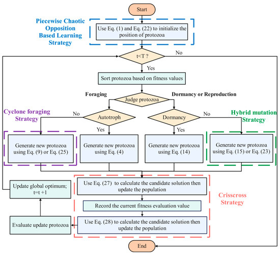
Figure 1.
Flowchart of MSAPO.
3.1. Piecewise Chaotic Opposition-Based Learning Strategy
The fundamental APO population initialization employs a random distribution, which is a straightforward approach but may result in an uneven spatial distribution of protozoan individuals. This, in turn, may prompt the algorithm to converge on a local optimum. To enhance the initial population quality of APO and circumvent the potential for local optimum convergence, piecewise chaotic opposition-based learning strategy is introduced in this section.
The fundamental premise of traditional OBL (opposition-based learning) is to derive the inverse solution to a feasible solution and select a superior candidate solution by evaluating the feasible solution and the inverse solution. The OBL formulation is as follows:
where represents the inverse solution corresponding to the ith individual in the random initial population. The application of OBL serves to facilitate the investigation of hitherto unconsidered solution domains within the search field, thereby enhancing the diversity of the population.
In an effort to more fully address the issue of unequal initial population distribution, this paper introduces the use of Piecewise chaotic mapping in OBL. Piecewise chaotic mapping is a segmentally defined chaotic system that divides the entire definition domain into multiple subintervals and applies distinct nonlinear transformations on each subinterval. This type of mapping is typically characterised by more intricate mathematical expressions and a greater degree of chaotic behavior, making it well suited to scenarios that demand heightened complexity and flexibility. The aforementioned mathematical model of piecewise chaotic mapping can be expressed as the following Equation (21),
where denotes the kth chaotic value of the Piecewise chaotic sequence , The preliminary value of the sequence is established by the random number rand, which is drawn from the interval , and chaos parameter .
The generation of chaotic sequences with a more balanced distribution is achieved through the application of Equation (21), which in turn is utilized to generate novel solutions, as illustrated in Equation (22),
where represents the novel solution, which is analogous to the initial population . signifies the corresponding sequence of chaotic mappings. Furthermore, the operator in this instance denotes the Hadamard product operation of two matrices.
Piecewise chaotic opposition-based learning strategy is utilized for the generation of a population of protozoa, which is then ranked and compared with the randomly generated population. The top superior individuals are subsequently selected as the initial population for subsequent operations. This strategy generates diverse populations through mirror flipping, retaining superior individuals as the initial population for iterative cycles. This approach enhances the diversity of the initial population and effectively prevents excessive clustering of the population near suboptimal positions. As this strategy operates solely during the initial population phase, it imposes minimal impact on the algorithm’s computational complexity.
3.2. Cyclone Foraging Strategy
In the autotrophic foraging phase, APO relies more on the guidance of random individuals to update the position. This process is exploratory but often accompanied by a high degree of blindness and randomness, resulting in a relatively slow speed of optimality search. In the heterotrophic foraging phase, the same characteristics will be observed. The algorithm is influenced by two types of individuals: those in nearby positions and the current individual’s front and rear neighbors, ranked according to the population’s fitness value. This can result in the algorithm reaching a local optimum, making it challenging to escape. To address this limitation, the cyclone foraging strategy [44] is integrated into the heterotrophic foraging phase of APO with the following mathematical model:
where is the position of the ith protozoa after updating in generation , is the optimal individual in the tth generation of protozoa. The random numbers and are drawn from a uniform distribution on the interval , and represents the weight coefficient.
Figure 2 illustrates the behavioral pattern of APO subsequent to the introduction of cyclone foraging strategy. The red blob in Figure 2 represents the current optimal protozoan individual, and the black blob represents the candidate individual. As shown in Figure 2, during the update process, APO’s is simultaneously influenced by and , generating a combined force along the spiral trajectory that propels the population toward the optimal point at an accelerated pace. In this way, APO updates its candidate individual of the population through the application of Equations (23) and (24), thereby approaching the optimal individual with the trajectory of the spiral line. The guidance of the global optimal individual enables APO to locate the search direction with greater accuracy, reducing the necessity for random wandering and significantly improving the speed of locating the optimal solution. Through the population renewal mechanism of cyclone foraging, individuals can approach the global optimum via richer convergence pathways. This enhances diversity in population renewal while maintaining incremental optimality, thereby preventing local optima traps.
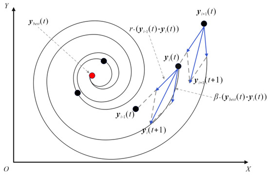
Figure 2.
Behavioral patterns of APOs after incorporating cyclone foraging strategy.
3.3. Hybrid Mutation Strategy
Figure 3 illustrates the variability of the density function curves of the standard Cauchy distribution (Cauchy (1,0)) and the standard Gaussian distribution (Gaussian (0,1)). In Figure 3, the Gaussian distribution and Cauchy distribution are continuous probability distributions that represent disturbance terms in nature. Their key difference lies in tail behavior: the Gaussian distribution exhibits exponential decay, resulting in rapid decreases in extreme outcomes, which characterizes it as a light-tailed distribution. In contrast, the Cauchy distribution has a power-law decay, which increases the likelihood of extreme outliers. In the Cauchy distribution, 1 denotes the scale parameter, which is half the width at half the maximum, while 0 denotes the position parameter, which is the peak of the distribution. In the Gaussian distribution, 0 is the mean and 1 is the standard deviation. With regard to the properties of probability distributions, the Cauchy distribution exhibits a greater probability of occurrence at both extremes, indicating a propensity for generating variance values that deviate from the origin. This makes it a more suitable choice for extensive searches in the initial stages of an iteration, whereas the Gaussian distribution displays a higher concentration near the origin, making it more appropriate for fine-tuning in the latter stages of an iteration.
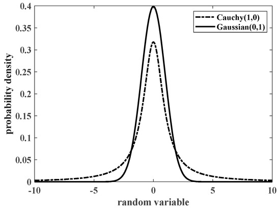
Figure 3.
Density profiles of the Cauchy and Gaussian distributions.
The hybrid mutation strategy employs the mixed mutation mechanism of Gaussian and Cauchy distributions to adjust the position of individuals with the objective of achieving diversification of mutation methods. The specific mathematical model is as follows:
where is the position of the individual after mutation, denotes a sequence of variants obeying Cauchy distribution, denotes a sequence of variants obeying Gaussian distribution. and denote the Cauchy and Gaussian variance factors, respectively, and the variations are shown in Figure 4. As shown in Figure 4, in the early stages of optimization, algorithms leverage outlier variance for exploration, and later transition to more minor errors for precise searches. Thus, parameters and , which sum to 1, are used to balance these two aspects of the algorithm.
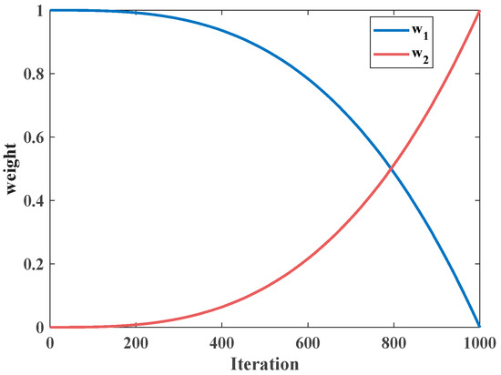
Figure 4.
Variation curves of weight factors w1 and w2 over 1000 iterations.
This paper introduces hybrid mutation strategy in the reproduction phase of the algorithm. By dynamically adjusting the weights of the Cauchy mutation factor and the Gaussian mutation factor, the algorithm is able to flexibly switch mutation modes during the iteration process, thereby achieving rapid escape from the local optimum in the early stage and accurate convergence in the later stage.
3.4. Crisscross Strategy
In order to circumvent the algorithm’s tendency to converge prematurely and to circumvent the potential pitfall of a local optimum, the APO introduces the Crisscross Strategy before the conclusion of the iteration [45]. The utilization of horizontal crossover in the search process can diminish the number of self-points encountered by the algorithm, thereby enhancing its global search capability. Vertical crossover, on the other hand, can facilitate the elimination of dimensions that have reached a point of convergence.
3.4.1. Horizontal Crossover
The horizontal crossover operation is analogous to the crossover operation in genetic algorithms, which facilitates the exchange of information between different populations in the same dimension. Initially, it is essential to randomly pair the individuals of the parents to perform the crossover operation in the dth dimension, as follows:
where and denote the values of the dth dimensional components of the two individuals and , respectively, produced by the ith protozoa and the jth protozoa in generation after a lateral crossover. is a random number between the interval [0, 1] and is a random number between the interval .
The solutions generated by the horizontal crossover must be evaluated in comparison with their parental counterparts, and the individuals exhibiting the highest degree of fitness are selected for retention. This approach guarantees the efficacy and precision of the algorithmic convergence and optimization.
3.4.2. Vertical Crossover
APO is prone to local optimality at a later stage, largely due to the fact that some individuals in the population exhibit local optimality in a specific dimension, which results in premature convergence of the entire system. To address this issue, MSAPO employs a strategy of horizontal and vertical crossover operations on newborn individuals, improving the algorithm’s capacity to circumvent local optima.
If we assume that newborn protozoan crosses vertically in the d1th and d2th dimensions, the calculation is as follows:
where is an individual resulting from vertical crossover from individual .
The vertical crossover process generates offspring individuals with enhanced fitness by integrating information from disparate dimensions. Furthermore, a meritocracy mechanism, as illustrated by Equation (29), is employed to guarantee the efficacy of the crossover operation. The conjunction of horizontal and vertical crossover results in augmented global search abilities and an enhanced capacity to circumvent local optima. In the iterative process, once an individual has escaped from a local optimum through vertical crossover, its updated dimension information is rapidly disseminated throughout the population via horizontal crossover, thereby driving the population as a whole towards a superior solution.
The pseudo code for MSAPO is given in Algorithm 2.
| Algorithm 2: MSAPO |
| Input: The population size N, the individual dimension D, Controlling parameters np, pfmax, and the maximum number of iterations T. |
| Output: The optimal individual ybest and its corresponding fitness fbest. |
 |
3.5. Computational Complexity
The basic APO performs sorting, dormancy and reproduction, autotrophic foraging and heterotrophic foraging, and fitness value calculations with a time complexity of . Piecewise chaotic opposition-based learning strategy adds the generation of the inverse solution of the chaotic mapping and the comparison of the ordering with the original initial population, with an increased time complexity of . The time complexity of the heterotrophic phase introducing cyclone foraging strategy increases . The time complexity of the hybrid mutation strategy is . The crisscross strategy has a time complexity of . To reduce the time complexity of the algorithm computation, the evaluation values are recorded once after the cross-sectional cross-computation, so the increased complexity of the computation of the fitness values that are retained optimally after the introduction of the strategy is . Therefore, the final time complexity of MSAPO is .
4. Numerical Experiments and Analysis
4.1. Baseline Algorithms and Benchmark Function Sets
In order to corroborate the enhanced performance of the MSAPO put forth in this paper, in this section, the CEC2017 and CEC2022 test sets are chosen for the purpose of conducting simulation experimentation and analyzing the resulting data. All functions of CEC2017 are rotated and shifted, increasing the difficulty of algorithmic optimization search. CEC2017 contains 29 test functions: unimodal functions (F1, F3), simple multimodal functions (F4–F10), hybrid functions (F11–F20), and composition functions (F21–F30). The CEC2022 test set includes 12 test functions. The unimodal function has only one global optimum, which is employed to assess the capability of the optimization algorithm to develop; the simple multimodal function contains multiple local optimums, which is utilized to evaluate the capacity of the algorithm to transcend the local optimum; and the hybrid function increases the complexity of the solution. Composition functions present more complex optimization problems and necessitate the utilization of algorithms with enhanced global exploration and local development capabilities. The efficacy of the optimization algorithm can be assessed in an objective manner through the utilization of test functions that encompass a diverse array of optimization problems.
The MSAPO algorithm is extensively compared with four classes of existing optimization algorithms: (1) The first class of algorithms: includes some well-known algorithms published in recent years, such as slime mold algorithm (SMA) [46], african vultures optimization algorithm (AVOA) [47], snake optimizer (SO) [25], artificial rabbits optimization (ARO) [48], nutcracker optimizer algorithm (NOA) [26] and PID-based search algorithm (PSA) [49]; (2) Algorithms in the second category: covering some widely cited and studied classical algorithms, including grey wolf optimizer (GWO) [21], whale optimization algorithm (WOA) [22] and salp swarm algorithm (SSA) [50]; (3) The third class of algorithms: includes variants of classical optimization algorithms PSO, such as XPSO [51], FVICLPSO [52] and SRPSO [53]; (4) Algorithms of the fourth category: including the high-performance optimizers LSHADE_cnEpSin [54] and LSHADE-SPACMA [55], which won the CEC2017 competition.
Initially, a comparison is made between MSAPO and the first three classes of algorithms under the highest dimension of the CEC2022 test set. To further validate the efficiency of MSAPO, experiments are conducted which include the fourth class of comparison algorithms under 30, 50 and 100 dimensions of the CEC2017 test set. In order to guarantee the comparability of the experimental results, the population size N of all algorithms was set to 100, and the maximum number of iterations set to 1000, corresponding to a maximum of 100,000 fitness evaluations. To eliminate the influence of chance factors, each algorithm was executed independently on 30 occasions.
In fact, we observed that certain algorithms employ strategies involving population reduction (such as LSHADE_cnEpSin and LSHADE_SPACMA). Some algorithms exhibit multiple evaluation behaviors (such as SO and NOA). For these algorithms, we recorded the fitness value corresponding to the global optimum after each evaluation. We then grouped these into 1000 sets of experimental data, each comprising 100 evaluations, thereby ensuring the fairness of the comparative trials.
4.2. Sensitivity Analysis of Parameter
In MSAPO, we introduce an additional chaotic parameter . To investigate whether the value of parameter significantly impacts algorithm performance and to determine its approximate optimal value, we conducted sensitivity analysis experiments on this parameter.
According to Equation (21), the parameter takes values within the range . Therefore, in this experiment, the candidate were set to 0.05, 0.1, …, 0.5. Table S1 presents the convergence curves of MSAPO under different parameter settings. According to Figure 5, the performance of MSAPO varies little across different parameters, indicating that the algorithm is not sensitive to the value of parameter . However, in the scenario where , the algorithm consistently achieves slightly better performance. Therefore, the default value of in this paper is set to 0.1.
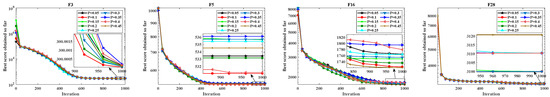
Figure 5.
Partial convergence curves in the sensitivity analysis experiment.
Table S1 shows the average values and rankings obtained using different values of the chaotic parameter () on the 30-dimensional CEC2017 test set. As indicated by the ranking in the last row of Table S1, MSAPO achieves the best overall ranking on the test set when . Therefore, the chaotic parameter is adopted for subsequent numerical experiments.
4.3. Ablation Experiment
MSAPO employs four strategies that collectively enhance its performance in complex engineering optimization. To validate their effectiveness, we conducted an experiment removing each strategy—named APO1, APO2, APO3, and APO4—representing the removal of 4 strategies, piecewise chaotic opposition-based learning strategy, cyclone foraging strategy, hybrid mutation strategy, and crisscross strategy. We performed ablation tests on a 30-dimensional CEC2017 dataset, comparing these algorithms with MSAPO.
Table 1 shows the average values of the optimal solutions for six algorithms, with partial convergence curves depicted in Figure 6. Results in Table 1 show the performance ranking: MSAPO > APO1 > APO2 > APO3 > APO4 > APO, indicating that removing any strategy reduces effectiveness. The crisscross strategy has the greatest impact on algorithm performance, while the chaotic opposition-based learning strategy has the least impact. The other two strategies also influence algorithm performance.

Table 1.
Statistical results of mean values in the melting experiment.
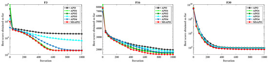
Figure 6.
Partial convergence curves in the ablation experiment.
4.4. Algorithm Parameter Settings and Performance Indicators
The parameter settings of the algorithms employed in the experiment are presented in Table 2. The paper employs five performance evaluation metrics to conduct a comprehensive analysis of the experimental results obtained from the MSAPO algorithm in comparison to other algorithms. These metrics encompass Mean, Best, standard deviation (Std), Mean Rank for Friedman’s test (MR), and Wilcoxon rank sum test for 30 runs on each test function.
Table 2.
Parameter settings of the experimental algorithms.
Mean and Best values provide an intuitive reflection of the efficacy of the algorithmic solution, whereas Std offers insight into the concentration of the solution results, thereby indicating the stability of the algorithmic solution. The ranking of each algorithm on the current test function can be derived by ranking the mean rank (MR) of the Friedman test. The Wilcoxon rank sum test provides a means of ascertaining whether the fitness values of the two algorithms originate from distributions with an identical median, thereby indicating whether they are significantly disparate. In this study, a one-sided Wilcoxon rank sum test was conducted on MSAPO and other comparison algorithms, with a significance level of 0.05. The calculated p-value allows us to statistically determine the performance of MSAPO on the test set in relation to its comparison algorithms. In the context of the Wilcoxon rank sum test, “+” signifies that the MSAPO algorithm is demonstrably superior to the comparison algorithm, “−” signifies that the MSAPO algorithm is significantly inferior to the comparison algorithm, and “=” signifies that there is no significant distinction between the two. The integration of these indicators offers a comprehensive and detailed reference point for the analysis of the experimental results.
4.5. Analysis of Results Under CEC2022
Table 3 and Table S2 present the statistical metrics of the 14 algorithms for the 12 test function optimization results under the 20-dimensional CEC2022 test set. The results include those of the Mean, Best, Std, MR, Rank and Wilcoxon rank-sum tests. Additionally, the table provides the average MR (Average MR) on the 12 test functions and the combined rank (Total Rank). As evidenced in Table 3 and Table S2, MSAPO exhibits the most optimal Mean performance across the eight test functions, F1, F3, F5–F9, and F12. It demonstrates the capacity to converge stably to its theoretical optimum on F1, F3, and F5, indicating a robust ability to navigate and overcome local optima. This makes MSAPO a versatile choice for diverse types of optimization problems. MSAPO achieved the smallest Std of all algorithms on functions F1, F3, F5, F6, F9, F10, and F12, showing the stability of its results. The results of the Wilcoxon rank sum test and the Rank metrics on the 12 tested functions indicate that MSAPO significantly outperforms the other compared algorithms on 10 functions and ranks first. Additionally, MSAPO achieves a second-place ranking on F4 and F10. With regard to function F4, APO exhibited a slight advantage over MSAPO, whereas FVICLPSO demonstrated superior performance on function F10. Collectively, MSAPO attained an average MR of 1.7500 across the 12 functions, ultimately securing the top ranking.
Table 3.
Comparison results of various algorithms under 20D CEC2022.
Figure 7 and Figure 8 illustrate the mean convergence curves and box plots of the 14 algorithms under the 20-dimensional CEC2022 test set. As illustrated in Figure 7, for the unimodal function F1, APO is unable to achieve a high convergence accuracy for the algorithm due to its slow convergence speed. In contrast, MSAPO expedites the convergence speed and optimality-finding ability of the algorithm through the utilization of a high-quality initial population and a hybrid mutation strategy, thereby enabling it to reach the optimal solution in a more rapid manner. In the context of the simple multimodal function F4, MSAPO’s principal competitor is APO. MSAPO demonstrates a superior convergence rate in the initial phase of the iteration, while APO exhibits a greater capacity to identify the optimal solution in the subsequent phase. Despite MSAPO’s inability to retain its leading position in this domain, the performance gap between it and APO remains relatively narrow. In addressing the intricate optimization issues pertaining to other combinatorial and composite functions within the test set, MSAPO has demonstrated its capacity to identify superior fitness values with a reduced number of iterations, thereby attaining enhanced convergence precision. This outcome suggests that MSAPO enhances the algorithmic convergence precision and its capacity to circumvent local optima through the deployment of cyclone foraging strategy and crisscross strategy. As illustrated in Figure 8, MSAPO exhibits the narrowest and lowest box across the majority of test functions, thereby substantiating its superior stability and optimality-finding capabilities. Figure 9 presents radar charts of the comprehensive ranking of MSAPO in comparison with other algorithms. The size of the enclosed area in the chart is indicative of the algorithm’s performance, allowing for an intuitive understanding of MSAPO’s notable superiority.
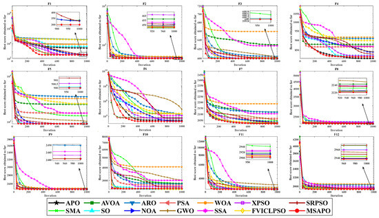
Figure 7.
Convergence curves of various algorithms under 20-dimensional CEC2022.
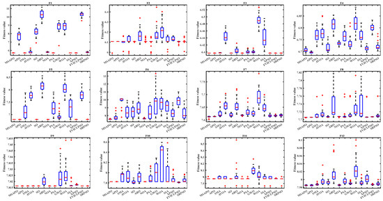
Figure 8.
Box plots of various algorithms under 20-dimensional CEC2022.
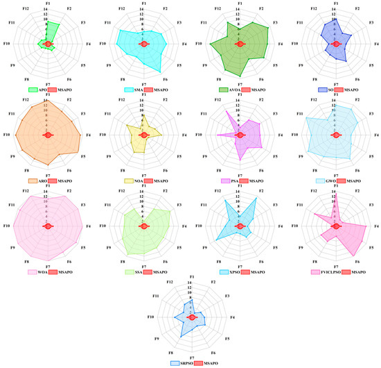
Figure 9.
Radar plots of the ranking of various algorithms under 20-dimensional CEC2022.
4.6. Result Analysis on CEC2017
In order to circumvent the constraints of a singular test set, this section elects to utilize CEC2017, which exhibits an analogous function type to that of CEC2022 and a more expansive array of optimization functions, as the test set. Additionally, it introduces two triumphant algorithms from the CEC2017 test set competition, LSHADE_cnEpSin and LSHADE_SPACMA, as the comparison algorithms to substantiate the efficacy of the proposed MSAPO algorithm. Table 4, Table 5, Table 6 and Tables S3–S5 present the Mean, Best, Std, MR, Rank, and Average MR and Total Rank of the 16 algorithms under the three dimensions and on 29 functions of the CEC2017 test set. Table 7, Table 8 and Table 9 show the statistical results of the Wilcoxon rank sum test with a significance level of 0.05.
Table 4.
Comparison results of 16 algorithms under 30-dimensional CEC2017.
Table 5.
Comparison results of 16 algorithms under 50-dimensional CEC2017.
Table 6.
Comparison results of 16 algorithms under 100-dimensional CEC2017.
Table 7.
Wilcoxon rank sum test results of MSAPO and other algorithms under 30-dimensional CEC2017.
Table 8.
Wilcoxon rank sum test results of MSAPO and other algorithms under 50-dimensional CEC2017.
Table 9.
Wilcoxon rank sum test results of MSAPO and other algorithms under 100-dimensional CEC2017.
The combined experimental results presented in Table 4, Table 5, Table 6 and Tables S3–S5 clearly illustrate that the MSAPO solution substantially exceeds the original APO for the 30-, 50-, and 100-dimensional unimodal functions F1 and F3 by orders of magnitude. In the 30- and 50-dimensional functions F1, MSAPO is ranked third, yet its Mean and Best metrics indicate that it identifies the theoretical optimum of the objective function. Furthermore, its overall performance is surpassed only by that of the two competition-winning algorithms. With a dimension of 100, MSAPO is the top-performing system in terms of F1. For function F3, MSAPO is the top-performing algorithm in all three dimensions, which indicates that the improvement strategy effectively enhances the exploration and development of the algorithm.
In the assessment of simple multimodal functions F4–F10, MSAPO achieved 3, 4 and 7 first places in 30, 50 and 100 dimensions, respectively. In 30 dimensions, MSAPO’s metrics on two functions exhibit slight inferiority compared to the original APO. However, in 50 and 100 dimensions, its overall performance is superior to the original APO, indicating that cyclone foraging strategy and crisscross strategy effectively enhance algorithm’s capacity to converge accurately and to circumvent local optima. As the dimension increases, MSAPO demonstrates a notable enhancement in its ability to solve problems, thereby indicating its efficacy in addressing complex, high-dimensional issues.
In the context of hybrid functions F11–F20, MSAPO achieved a total of 7, 6, and 6 first-place rankings in 30, 50, and 100 dimensions, respectively. In the 30-dimensional experiment, MSAPO ranked third on function F12, with two competition winning algorithms as the main competitors. In regard to function F14, while MSAPO’s Mean and Std metrics are not as good as those of the original APO, its best metrics demonstrate superior performance, indicating an aptitude for identifying optimal outcomes. However, further enhancements are necessary to ensure stability. In regard to function F18, MSAPO’s performance is surpassed only by the two competition-winning algorithms. In the 50-dimensional experiments, MSAPO’s overall performance on function F12 is second only to LSHADE_SPACMA, but it excels in its Best metric. In terms of functions F14 and F18, MSAPO is ranked third, which is below the two competition-winning algorithms. In the ranking of function F15, APO, NOA, XPSO, LSHADE_cnEpSin and LSHADE_SPACMA demonstrated superior performance. In the 100-dimensional experiments, MSAPO ranked in the top three of all 10 hybrid functions, with individual functions not as good as the statistical metrics of the two competition-winning algorithms.
In the composition functions F21–F30, MSAPO obtained 2, 8 and 9 first places in 30, 50 and 100 dimensions, respectively. In 30 dimensions, APO demonstrates superior performance to MSAPO on five functions, indicating that APO is a more advantageous approach for addressing low-dimensional complex problems. In 50 dimensions, MSAPO demonstrates superior performance to the original APO across all metrics on 10 functions. However, it is ranked third behind the two competing algorithms on function F18 and exhibits suboptimal performance on function F25, where it is ranked eighth. In the 100-dimensional function F26, MSAPO is outperformed by XPSO and SRPSO. However, its Mean, Best, and Std exceed those of the other algorithms, indicating that MSAPO’s overall performance remains superior.
Table 7, Table 8 and Table 9 illustrate the Wilcoxon rank sum test statistics between MSAPO and the other 15 algorithms, evaluated in three dimensions. Table 7 illustrates that out of the 29 test functions of the 30-dimensional CEC2017, MSAPO performed better on 20 functions, comparable on 5 functions, and worse on 4 functions compared to the original APO. MSAPO’s principal competitors are LSHADE_cnEpSin and LSHADE_SPACMA, with MSAPO exhibiting inferior performance relative to LSHADE_cnEpSin on eight functions and to LSHADE_SPACMA on 11. In comparison to the other algorithms that were subjected to evaluation, MSAPO demonstrated superior performance across all 29 functions that were tested.
The 50-dimensional experimental results presented in Table 8 show that MSAPO’s performance is significantly improved compared to the 30-dimensional. Specifically, 27 functions demonstrate a performance that is superior to that of the original APO, while one function exhibits a performance that is comparable to that of the original APO, and one function exhibits a performance that is inferior to that of the original APO. However, MSAPO is significantly inferior to SMA and SRPSO on F25, to SO on F5, F8, and to NOA and XPSO on F15. For LSHADE_cnEpSin and LSHADE_SPACMA, MSAPO is inferior to LSHADE_cnEpSin on 4 functions, and to LSHADE_ SPACMA. Overall, there is still scope for enhancement in MSAPO’s optimised performance on F5, F7, F8, F15, F18 and F25.
The 100-dimensional test results presented in Table 9 demonstrate that MSAPO exhibits enhanced performance, significantly outperforming the original APO on 28 test functions. There is no discernible difference between MSAPO and APO on F19, and MSAPO identifies a superior Best. With the exception of F14 and F18, where the performance is not as optimal as that of LSHADE_cnEpSin and LSHADE_SPACMA, MSAPO demonstrates superior performance to the comparative algorithms across the remaining functions, thereby substantiating its robust capability in addressing high-dimensional optimization problems.
The Friedman average ranking data for the 29 functions in Table 4, Table 5, Table 6 and Tables S3–S5 were combined to produce the final rankings on the 30-, 50-, and 100-dimensions for MSAPO. These were found to be 2.6460, 2.5103, and 1.9046, respectively, which all rank first. In general, MSAPO demonstrates superior performance compared to the other 15 algorithms on all three dimensions of the CEC2017 test set. This illustrates its robust capability for optimization, particularly in complex high-dimensional optimization problems where it exhibits remarkable proficiency in optimization finding.
Furthermore, the convergence and stability of MSAPO are illustrated by the convergence curves and box plots of the 16 algorithms, and the convergence curves of the 16 algorithms on 29 test functions in 30, 50 and 100 dimensions are presented in Figure 10, Figure 11 and Figure 12, respectively. The convergence curves demonstrate that MSAPO exhibits a faster convergence rate than APO during the pre-iteration period. Furthermore, MSAPO identifies superior fitness values and attains higher convergence accuracy with a reduced number of iterations. In particular, the convergence performance of MSAPO is more pronounced in 100 dimensions than in 30 and 50 dimensions. The box plots for the three dimensions are provided in Figure 13, Figure 14, and Figure 15, respectively. The MSAPO exhibits the narrowest and lowest box in the case of the majority of the test functions, which indicates that it demonstrates superior stability and optimization-seeking ability.
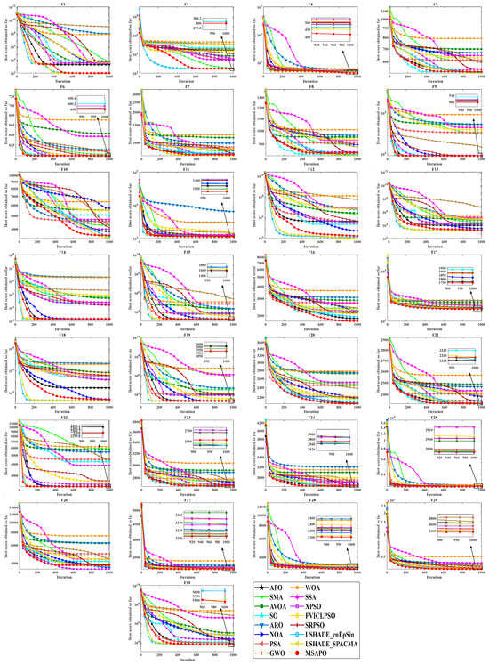
Figure 10.
Convergence curves of various algorithms under 30-dimensional CEC2017.
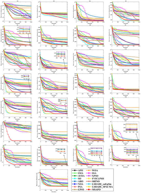
Figure 11.
Convergence curves of various algorithms under 50-dimensional CEC2017.
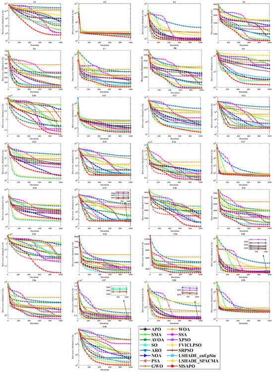
Figure 12.
Convergence curves of various algorithms under 100-dimensional CEC2017.
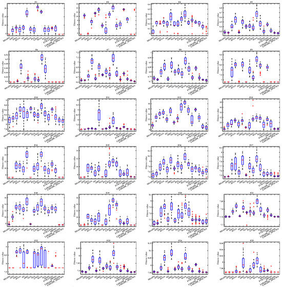
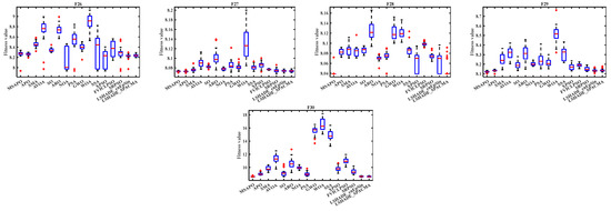
Figure 13.
Box plots of various algorithms under 30-dimensional CEC2017.
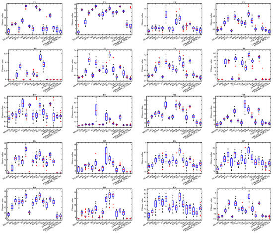
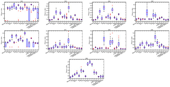
Figure 14.
Box plots of various algorithms under 50-dimensional CEC2017.
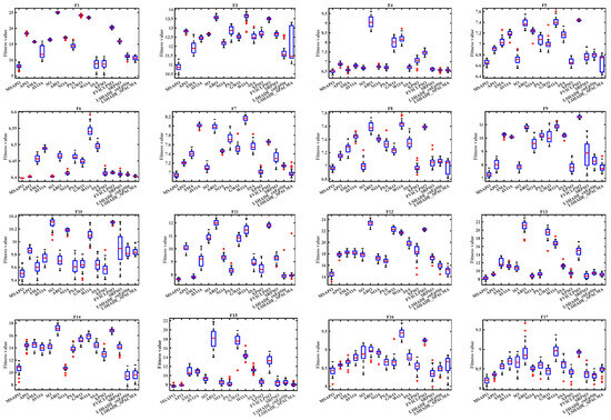
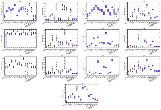
Figure 15.
Box plots of various algorithms under 100-dimensional CEC2017.
4.7. Result Analysis on CEC2017
In this section, we conducted three independent numerical experiments using MSAPO. In the first experiment, we performed a sensitivity analysis on the newly added parameter P in MSAPO. The results indicate that changes in parameter P have little impact on the algorithm’s stability. When P is set to 0.1, the algorithm exhibits a slight advantage in convergence accuracy compared to other parameter values. In the second set of experiments, we sequentially removed each strategy component from MSAPO to validate the rationality of their combination. Results confirmed that every strategy component contributes positively to the algorithm, and the combined strategy set significantly outperforms the original algorithm. We compared the performance of MSAPO with optimized parameter P against dozens of benchmark algorithms. These benchmarks encompassed a comprehensive range of types, with standardized environments and parameter settings to ensure fairness and consistency across all evaluations. Experimental results demonstrate that MSAPO exhibits high convergence speed and accuracy, maintains exceptional stability across diverse test functions, and holds significant potential for tackling complex optimization problems in engineering.
5. Real-World Optimization Problems
This section employs MSAPO and 13 comparative algorithms (presented in Section 4.3) to address a set of 8 real-world constrained optimization problems [56]. The objective is to evaluate the efficacy of MSAPO in addressing engineering design optimization problems. The parameters of the given engineering problems are presented in Table 10. In order to evaluate the results yielded by each algorithm, four statistical indicators are employed: Best, Mean, Worst, and Std. The eight engineering constraint problems have different mathematical models and constraints, allowing for the effective testing of the algorithms’ ability and applicability in solving these problems. To facilitate a fair and consistent comparison, the population size, the number of independent runs of the algorithms, and the Maximum iteration times of the 14 algorithms are maintained at the same values throughout the process, which are set at 30, 30, and 500, respectively.
Table 10.
Parameters of engineering problems.
5.1. Process Synthesis Problem (PSP)
PSP can be defined as a mixed-integer nonlinear constrained optimization problem [56]. The problem comprises 7 free variables () and 9 nonlinear constraints (). The mathematical model is as follows:
subject to:
where the range of the variables are , .
The numerical results obtained for the 14 algorithms employed to solve PSP are presented in Table 11 and Table S6. The optimal values are indicated by bold text in the tables, and the engineering problems that follow are similarly labelled. Table 11 illustrates that MSAPO’s Best and Worst are the smallest among all algorithms. Notably, MSAPO’s Best reaches the theoretical optimum of 2.9248305537 for PSP, which suggests that MSAPO has the capacity to resolve this specific issue in an exemplary manner. The inferior performance of MSAPO in comparison to NOA on Mean and Std indicates that MSAPO lacks the reliability and robustness necessary to effectively address PSP. The statistical indicators of MSAPO are superior to those of the original APO, which suggests that the incorporation of the four strategies has led to a notable enhancement in the algorithm’s performance. Table S6 presents the optimal design solution for PSP solved by MSAPO, which is (0.1983, 1.2806, 1.9547, 0.7564, −0.4323, 0.0864, 1.2050).
Table 11.
Statistical results of PSP.
5.2. Weight Minimization of a Speed Reducer (WMSR)
The objective of WMSR is the design of a reducer for a small aircraft engine. In order to minimise the weight of the reducer, WMSR must satisfy 11 constraints, involving 7 variables. Figure 16 shows the schematic structure of the reducer and the specific mathematical model of the problem is as follows:
subject to:
where the range of the variables are , , , , , .
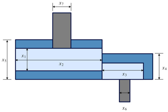
Figure 16.
The speed reducer design model.
The numerical results obtained for the 14 algorithms used to solve WMSR are presented in Table 12 and Table S7. Table 12 demonstrates that the optimal value of 2994.4244658 for WMSR can be reached by Best, Mean and Worst of MSAPO. Furthermore, Std outperforms the other comparative algorithms, indicating that MSAPO is an effective and robust method for solving WMSR. It is also concerned that PSA and FVICLPSO can also solve for the theoretical optimum, suggesting that they converge with sufficient accuracy, but neither is as robust as MSAPO. Table S7 illustrates the optimal design solution as determined by MSAPO. The solution is (3.5, 0.7, 17, 7.3, 7.7153, 3.3505, 5.2867).
Table 12.
Statistical results of WMSR.
5.3. Tension/Compression Spring Design (T/CSD)
In the context of T/CSD, the objective is to minimise the weight of the tension/compression spring. The schematic structure is illustrated in Figure 17. The problem mainly consists of 3 continuous decision variables, and 4 constraints are to be satisfied, which are mathematically modelled as follows:
subject to:
where the range of the variables are , , .
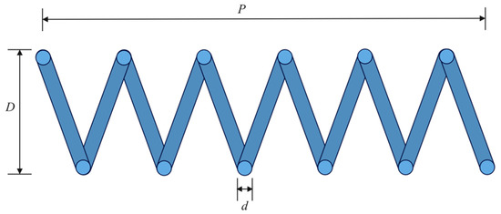
Figure 17.
Schematic diagram of T/CSD.
The numerical results obtained for the 14 algorithms used to solve T/CSD are shown in Table 13 and Table S8. Table 13 illustrates that Best of MSAPO is the smallest among all the algorithms and attaining the theoretical optimum of 0.0126652328 for T/CSD. However, the performance of MSAPO on Mean, Worst and Std is not as good as that of NOA, which indicates that the reliability and robustness of MSAPO for T/CSD are still insufficient. Table S8 indicates that the optimal design solution for the T/CSD solved by MSAPO is (0.0516875570, 0.3566815558, 11.2910874220).
Table 13.
Statistical Results of T/CSD.
5.4. Welded Beam Design (WBD)
The objective of WBD [57] is to find the lowest solution for the manufacturing cost by adjusting the decision variables. The configuration of WBD is depicted in Figure 18, which contains 4 design variables and 5 constraints and is mathematically modelled as follows:
subject to:
where:
with bounds: , , .
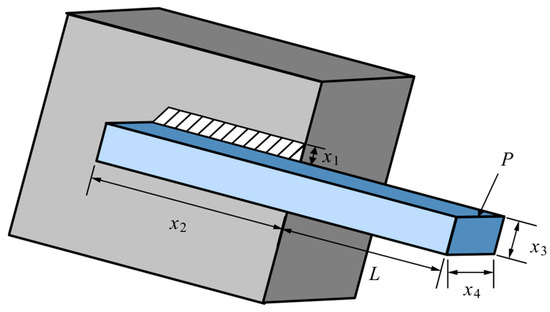
Figure 18.
Schematic design of welded beam [57].
The numerical results obtained for the 14 algorithms employed to solve WBD are presented in Table 14 and Table S9. Table 14 shows that the MSAPO Best, Mean and Worst values reach the theoretical optimum of 1.6702177263 for WBD, and that its standard deviation is also significantly better than that of the other algorithms under comparison. Although XPSO’s Best can also reach the theoretical optimum, it is less stable. Table S9 indicates that the best design solution for WBD solved by MSAPO is (0.1988323072, 3.3373652986, 9.1920243225, 0.1988323072).
Table 14.
Statistical results of WBD.
5.5. Three-Bar Truss Design Problem (TBTD)
In the context of TBTD, the primary objective is to minimise the volume of the three-rod truss, as illustrated schematically in Figure 19. Given that the cross-sectional areas of rods and are identical in the three-rod truss, only rods and are selected as the optimization variables, and the variable represents the stress that the three-rod truss is subjected to at each truss member. The particular mathematical model is as follows:
subject to:
where
with bounds: .
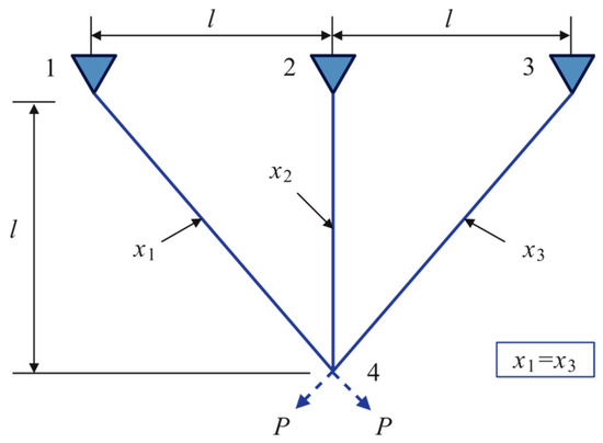
Figure 19.
Schematic diagram of TBTD.
The numerical results obtained for the 14 algorithms used to solve TBTD are presented in Table 15 and Table S10. Table 15 illustrates that the three algorithms, MSAPO, APO and NOA, collectively achieved the theoretical optimum value of 263.89584338 for TBTD. Nevertheless, MSAPO displays superior performance in terms of Mean, Worst and Std metrics in comparison to the other algorithms. Table S10 indicates that the optimal design solution for TBTD solved by MSAPO is (0.7886751377, 0.4082482817).
Table 15.
Statistical results of TBTD.
5.6. Step-Cone Pulley Problem (SCP)
The main objective of SCP [58] is to minimise the weight of a 4th order conical pulley using 5 variables. This problem contains 11 nonlinear constraints. The structure of step-cone pulley is shown schematically in Figure 20. The formula is as follows:
subject to:
where and is the belt length to obtain speed , and respectively represents the tension ratio and the power transmitted at each step, the formulas are as follows
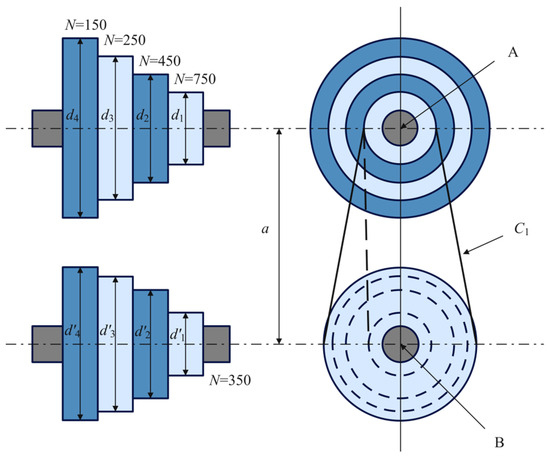
Figure 20.
Schematic diagram of SCP.
The numerical results obtained for the 14 algorithms used to solve SCP are given in Table 16 and Table S11. As illustrated in Table 16, the MSAPO exhibits superior performance in terms of the Best and Mean metrics when compared to the other algorithms. However, according to the Std metric, it displays slightly reduced stability. The optimal design solution solved by MSAPO in Table S11 is (38.41396, 52.85864, 70.47270, 84.49572, 90).
Table 16.
Statistical results of SCP.
5.7. Gas Transmission Compressor Design (GTCD)
GTCD [59] has 4 decision variables and 1 constraint. The specific mathematical model is as follows:
subject to:
with bounds: , , .
The numerical results obtained for the 14 algorithms employed to address GTCD are presented in Table 17 and Table S12. Table 17 illustrates that Best metric of three algorithms, MSAPO, APO and NOA, is the smallest among the compared algorithms. Meanwhile, Mean, Worst and Std metrics of MSAPO demonstrate a notable superiority over those of the other algorithms. Table S12 denotes that the optimal design solution for GTCD solved by MSAPO is (50, 1.178283951, 24.592590288, 0.388353071).
Table 17.
Statistical results of GTCD.
5.8. Himmelblau’s Function (HF)
Himmelblau’s function is a general benchmark for the analysis of nonlinear constrained optimization algorithms [56], comprising 6 nonlinear constraints and 5 variables. The specific modelling of the problem is as follows:
subject to:
where
with bounds: , , .
Table 18 and Table S13 present the results of 14 algorithms to solve Himmelblau’s function. Table 18 demonstrates that MSAPO’s Best, Mean, and Worst values align with the Himmelblau’s function theoretical optimal value of −30665.538672. Additionally, MSAPO’s Std value exhibits a notable superiority over those of other algorithms, indicating that MSAPO possesses exceptional capabilities in solving Himmelblau’s function. From Table S13, the optimal design solution for Himmelblau’s function solved by MSAPO is (78, 33, 29.99525603, 45, 36.77581291).
Table 18.
Statistical results of Himmelblau’s function.
5.9. Conclusion on Engineering Optimization Problems
In the section addressing practical engineering optimization problems, we conducted eight independent experiments, each corresponding to a distinct engineering optimization problem. Across these experiments, MSAPO demonstrated superior overall performance in most problems, ranking highly across the majority of evaluation metrics. Benefiting from the enhancement provided by the cross-strategy approach, MSAPO exhibits the ability to avoid local optima. Furthermore, its cyclonic search pattern accelerates convergence speed in high-dimensional problems. However, while the algorithm achieved competitive optimality in a few optimization problems, it exhibited weaker stability compared to algorithms like NOA in certain low-dimensional complex constraint problems (e.g., process synthesis, stepped cone pulleys). Consequently, there remains room for improvement in this algorithm.
6. Conclusions and Future Work
This paper proposes an enhanced APO algorithm, designated MSAPO, which incorporates piecewise chaotic opposition-based learning strategy, cyclone foraging strategy, hybrid mutation strategy, and crisscross strategy, alongside the APO. The combination of these four strategies enhances the initial population diversity, augment the local search capability of the algorithm, and diminish the probability of the algorithm attaining a local optimum. The comparison of the results with other excellent optimization algorithms on the CEC2017 and CEC2022 test functions reveals that the proposed MSAPO has significantly enhanced its computational accuracy and convergence speed. Notably, MSAPO demonstrates a remarkable capacity to identify optimal solutions, particularly in high-dimensional problems, which substantiates its competitiveness in optimization problems. The experimental results of the engineering examples demonstrate that MSAPO is capable of identifying superior optimization solutions when confronted with genuine problems. Nevertheless, MSAPO is not without its own set of limitations. The incorporation of the vertical and horizontal crossover strategy towards the conclusion of the algorithmic process has the effect of increasing its overall complexity, thereby rendering it less optimal for achieving rapid convergence when confronted with specific functional equations. In the future, the algorithm’s problem-solving ability will be enhanced by incorporating a variety of strategies to address diverse types of problems. Furthermore, the potential of the proposed MSAPO to optimize intricate optimization problems in diverse fields represents a promising avenue for future research.
Supplementary Materials
The following supporting information can be downloaded at: https://www.mdpi.com/article/10.3390/math13172888/s1, Table S1: Experimental results for different P values under 30-dimensional CEC2017; Table S2: Comparison results of various algorithms under 20-dimensional cec2022; Table S3: Comparison results of 16 algorithms under 30-dimensional cec2017; Table S4: Comparison results of 16 algorithms under 50-dimensional cec2017; Table S5: Comparison results of 16 algorithms under 100-dimensional cec2017; Table S6: Optimal design solutions for process synthesis problem; Table S7: Optimal design solutions for weight minimization of a speed reducer; Table S8: Optimal design solutions for tension/compression spring design; Table S9: Optimal design solution for welded beam design; Table S10: Optimal design solution for three-bar truss design problem; Table S11: Optimal design solution for step-cone pulley problem; Table S12: Optimal design solutions for gas transmission compressor design; Table S13: Optimal design solutions for himmelblau’s function.
Author Contributions
Conceptualization, G.H.; Methodology, H.B., J.W. and G.H.; Software, H.B. and J.W.; Validation, J.W. and G.H.; Formal analysis, H.B.; Investigation, H.B., J.W. and G.H.; Resources, G.H.; Data curation, H.B. and J.W.; Writing—original draft, H.B., J.W. and G.H.; Writing—review and editing, H.B., J.W. and G.H.; Visualization, J.W.; Supervision, G.H.; Project administration, G.H.; Funding acquisition, G.H. All authors have read and agreed to the published version of the manuscript.
Funding
This research received no external funding.
Data Availability Statement
The original contributions presented in this study are included in the article/Supplementary Materials. Further inquiries can be directed to the corresponding author.
Conflicts of Interest
The authors declare no conflicts of interest.
References
- Yao, L.; Yuan, P.; Tsai, C.Y.; Zhang, T.; Lu, Y.; Ding, S. ESO: An enhanced snake optimizer for real-world engineering problems. Expert Syst. Appl. 2023, 230, 120594. [Google Scholar] [CrossRef]
- Elnokrashy, A.F.; Abdelaziz, L.N.; Shawky, A.; Tawfeek, R.M. Advanced framework for enhancing ultrasound images through an optimized hybrid search algorithm and a novel motion compounding processing chain. Biomed. Signal Process. Control 2023, 86, 105237. [Google Scholar] [CrossRef]
- Abdel-Salam, M.; Alzahrani, A.I.; Alblehai, F.; Zitar, R.A.; Abualigah, L. An improved Genghis Khan optimizer based on enhanced solution quality strategy for global optimization and feature selection problems. Knowl.-Based Syst. 2024, 302, 112347. [Google Scholar] [CrossRef]
- Ming, F.; Gong, W.; Zhen, H.; Wang, L.; Gao, L. Constrained multi-objective optimization evolutionary algorithm for real-world continuous mechanical design problems. Eng. Appl. Artif. Intell. 2024, 135, 108673. [Google Scholar] [CrossRef]
- Hu, G.; Zhong, J.; Du, B.; Guo, W. An enhanced hybrid arithmetic optimization algorithm for engineering applications. Comput. Methods Appl. Mech. Eng. 2022, 394, 114901. [Google Scholar] [CrossRef]
- Houssein, E.H.; Çelik, E.; Mahdy, M.A.; Ghoniem, R.M. Self-adaptive Equilibrium Optimizer for solving global, combinatorial, engineering, and Multi-Objective problems. Expert Syst. Appl. 2022, 195, 116552. [Google Scholar] [CrossRef]
- Luo, W.; Yu, X. Reinforcement learning-based modified cuckoo search algorithm for economic dispatch problems. Knowl.-Based Syst. 2022, 257, 109844. [Google Scholar] [CrossRef]
- Liang, S.; Yin, M.; Sun, G.; Li, J.; Li, H.; Lang, Q. An enhanced sparrow search swarm optimizer via multi-strategies for high-dimensional optimization problems. Swarm Evol. Comput. 2024, 88, 101603. [Google Scholar] [CrossRef]
- Lu, H.C.; Tseng, H.Y.; Lin, S.W. Double-track particle swarm optimizer for nonlinear constrained optimization problems. Inf. Sci. 2023, 622, 587–628. [Google Scholar] [CrossRef]
- Meng, X.; Li, H. An adaptive co-evolutionary competitive particle swarm optimizer for constrained multi-objective optimization problems. Swarm Evol. Comput. 2024, 91, 101746. [Google Scholar] [CrossRef]
- Zhao, S.; Zhang, T.; Ma, S.; Wang, M. Sea-horse optimizer: A novel nature-inspired meta-heuristic for global optimization problems. Appl. Intell. 2023, 53, 11833–11860. [Google Scholar] [CrossRef]
- Hu, G.; Cheng, M.; Houssein, E.H.; Hussien, A.G.; Abualigah, L. SDO: A novel sled dog-inspired optimizer for solving engineering problems. Adv. Eng. Inform. 2024, 62, 102783. [Google Scholar] [CrossRef]
- Hamarashid, H.K.; Hassan, B.A.; Rashid, T.A. Modified-improved fitness dependent optimizer for complex and engineering problems. Knowl.-Based Syst. 2024, 300, 112098. [Google Scholar] [CrossRef]
- Bohrer, J.D.S.; Dorn, M. Enhancing classification with hybrid feature selection: A multi-objective genetic algorithm for high-dimensional data. Expert Syst. Appl. 2024, 255, 124518. [Google Scholar] [CrossRef]
- Storn, R.; Price, K. Differential evolution—A simple and efficient heuristic for global optimization over continuous spaces. J. Glob. Optim. 1997, 11, 341–359. [Google Scholar] [CrossRef]
- Civicioglu, P. Backtracking Search Optimization Algorithm for numerical optimization problems. Appl. Math. Comput. 2013, 219, 8121–8144. [Google Scholar] [CrossRef]
- Serrano-Rubio, J.P.; Hernández-Aguirre, A.; Herrera-Guzmán, R. An evolutionary algorithm using spherical inversions. Soft Comput. 2018, 22, 1993–2014. [Google Scholar] [CrossRef]
- Segovia-Domínguez, I.; Herrera-Guzmán, R.; Serrano-Rubio, J.P.; Hernández-Aguirre, A. Geometric probabilistic evolutionary algorithm. Expert Syst. Appl. 2020, 144, 113080. [Google Scholar] [CrossRef]
- Al-Bahrani, L.T.; Patra, J.C. A novel orthogonal PSO algorithm based on orthogonal diagonalization. Swarm Evol. Comput. 2018, 40, 1–23. [Google Scholar] [CrossRef]
- Dorigo, M.; Birattari, M.; Stutzle, T. Ant colony optimization. IEEE Comput. Intell. Mag. 2006, 1, 28–39. [Google Scholar] [CrossRef]
- Mirjalili, S.; Mirjalili, S.M.; Lewis, A. Grey Wolf Optimizer. Adv. Eng. Softw. 2014, 69, 46–61. [Google Scholar] [CrossRef]
- Mirjalili, S.; Lewis, A. The Whale Optimization Algorithm. Adv. Eng. Softw. 2016, 95, 51–67. [Google Scholar] [CrossRef]
- Heidari, A.A.; Mirjalili, S.; Faris, H.; Aljarah, I.; Mafarja, M.; Chen, H. Harris hawks optimization: Algorithm and applications. Future Gener. Comput. Syst. 2019, 97, 849–872. [Google Scholar] [CrossRef]
- Faramarzi, A.; Heidarinejad, M.; Mirjalili, S.; Gandomi, A.H. Marine Predators Algorithm: A nature-inspired metaheuristic. Expert Syst. Appl. 2020, 152, 113377. [Google Scholar] [CrossRef]
- Hashim, F.A.; Hussien, A.G. Snake Optimizer: A novel meta-heuristic optimization algorithm. Knowl.-Based Syst. 2022, 242, 108320. [Google Scholar] [CrossRef]
- Abdel-Basset, M.; Mohamed, R.; Jameel, M.; Abouhawwash, M. Nutcracker optimizer: A novel nature-inspired metaheuristic algorithm for global optimization and engineering design problems. Knowl.-Based Syst. 2023, 262, 110248. [Google Scholar] [CrossRef]
- Hu, G.; Guo, Y.; Wei, G.; Abualigah, L. Genghis Khan shark optimizer: A novel nature-inspired algorithm for engineering optimization. Adv. Eng. Inf. 2023, 58, 102210. [Google Scholar] [CrossRef]
- Abdel-Basset, M.; Mohamed, R.; Abouhawwash, M. Crested Porcupine Optimizer: A new nature-inspired metaheuristic. Knowl.-Based Syst. 2024, 284, 111257. [Google Scholar] [CrossRef]
- Fu, Y.; Liu, D.; Chen, J.; He, L. Secretary bird optimization algorithm: A new metaheuristic for solving global optimization problems. Artif. Intell. Rev. 2024, 57, 123. [Google Scholar] [CrossRef]
- Rao, R.V.; Savsani, V.J.; Vakharia, D.P. Teaching-learning-based optimization: A novel method for constrained mechanical design optimization problems. Comput.-Aided Des. 2011, 43, 303–315. [Google Scholar] [CrossRef]
- Das, B.; Mukherjee, V.; Das, D. Student psychology based optimization algorithm: A new population based optimization algorithm for solving optimization problems. Adv. Eng. Softw. 2020, 146, 102804. [Google Scholar] [CrossRef]
- Moosavi, S.H.S.; Bardsiri, V.K. Poor and rich optimization algorithm: A new human-based and multi populations algorithm. Eng. Appl. Artif. Intell. 2019, 86, 165–181. [Google Scholar] [CrossRef]
- Mohamed, A.W.; Hadi, A.A.; Mohamed, A.K. Gaining-sharing knowledge based algorithm for solving optimization problems: A novel nature-inspired algorithm. Int. J. Mach. Learn. Cybern. 2020, 11, 1501–1529. [Google Scholar] [CrossRef]
- Zhu, D.; Wang, S.; Zhou, C.; Yan, S.; Xue, J. Human memory optimization algorithm: A memory-inspired optimizer for global optimization problems. Expert Syst. Appl. 2024, 237, 121597. [Google Scholar] [CrossRef]
- Mirjalili, S. SCA: A Sine Cosine Algorithm for solving optimization problems. Knowl.-Based Syst. 2016, 96, 120–133. [Google Scholar] [CrossRef]
- Bouchekara, H.R. Electrostatic discharge algorithm: A novel nature-inspired optimisation algorithm and its application to worst-case tolerance analysis of an EMC filter. IET Sci. Meas. Technol. 2019, 13, 491–499. [Google Scholar] [CrossRef]
- Hashim, F.A.; Hussain, K.; Houssein, E.H.; Mabrouk, M.S.; Al-Atabany, W. Archimedes optimization algorithm: A new metaheuristic algorithm for solving optimization problems. Appl. Intell. 2021, 51, 1531–1551. [Google Scholar] [CrossRef]
- Deng, L.; Liu, S. Snow ablation optimizer: A novel metaheuristic technique for numerical optimization and engineering design. Expert Syst. Appl. 2023, 225, 120069. [Google Scholar] [CrossRef]
- Hashim, F.A.; Mostafa, R.R.; Hussien, A.G.; Mirjalili, S.; Sallam, K.M. Fick’s Law Algorithm: A physical law-based algorithm for numerical optimization. Knowl.-Based Syst. 2023, 260, 110146. [Google Scholar] [CrossRef]
- Hu, G.; Gong, C.; Li, X.; Xu, Z. CGKOA: An enhanced Kepler optimization algorithm for multi-domain optimization problems. Comput. Methods Appl. Mech. Eng. 2024, 425, 116964. [Google Scholar] [CrossRef]
- Duan, Y.; Yu, X. A collaboration-based hybrid GWO-SCA optimizer for engineering optimization problems. Expert Syst. Appl. 2023, 213, 119017. [Google Scholar] [CrossRef]
- Wolpert, D.H.; Macready, W.G. No free lunch theorems for optimization. IEEE Trans. Evol. Comput. 1997, 1, 67–82. [Google Scholar] [CrossRef]
- Wang, X.; Snášel, V.; Mirjalili, S.; Pan, J.S.; Kong, L.; Shehadeh, H.A. Artificial Protozoa Optimizer (APO): A novel bio-inspired metaheuristic algorithm for engineering optimization. Knowl.-Based Syst. 2024, 295, 111737. [Google Scholar] [CrossRef]
- Zhao, W.; Zhang, Z.; Wang, L. Manta ray foraging optimization: An effective bio-inspired optimizer for engineering applications. Eng. Appl. Artif. Intell. 2020, 87, 103300. [Google Scholar] [CrossRef]
- Chakraborty, S.; Saha, A.K.; Ezugwu, A.E.; Chakraborty, R.; Saha, A. Horizontal crossover and co-operative hunting-based Whale Optimization Algorithm for feature selection. Knowl.-Based Syst. 2023, 282, 111108. [Google Scholar] [CrossRef]
- Li, S.; Chen, H.; Wang, M.; Heidari, A.A.; Mirjalili, S. Slime mould algorithm: A new method for stochastic optimization. Future Gener. Comput. Syst. 2020, 111, 300–323. [Google Scholar] [CrossRef]
- Abdollahzadeh, B.; Gharehchopogh, F.S.; Mirjalili, S. African vultures optimization algorithm: A new nature-inspired metaheuristic algorithm for global optimization problems. Comput. Ind. Eng. 2021, 158, 107408. [Google Scholar] [CrossRef]
- Wang, L.; Cao, Q.; Zhang, Z.; Mirjalili, S.; Zhao, W. Artificial rabbits optimization: A new bio-inspired meta-heuristic algorithm for solving engineering optimization problems. Eng. Appl. Artif. Intell. 2022, 114, 105082. [Google Scholar] [CrossRef]
- Gao, Y. PID-based search algorithm: A novel metaheuristic algorithm based on PID algorithm. Expert Syst. Appl. 2023, 232, 120886. [Google Scholar] [CrossRef]
- Mirjalili, S.; Gandomi, A.H.; Mirjalili, S.Z.; Saremi, S.; Faris, H.; Mirjalili, S.M. Salp Swarm Algorithm: A bio-inspired optimizer for engineering design problems. Adv. Eng. Softw. 2017, 114, 163–191. [Google Scholar] [CrossRef]
- Xia, X.; Gui, L.; He, G.; Wei, B.; Zhang, Y.; Yu, F.; Wu, H.; Zhan, Z.H. An expanded particle swarm optimization based on multi-exemplar and forgetting ability. Inf. Sci. Int. J. 2020, 508, 105–120. [Google Scholar] [CrossRef]
- Xu, S.; Xiong, G.; Mohamed, A.W.; Bouchekara, H.R. Bouchekara, Forgetting velocity based improved comprehensive learning particle swarm optimization for non-convex economic dispatch problems with valve-point effects and multi-fuel options. Energy 2022, 256, 124511. [Google Scholar] [CrossRef]
- Tanweer, M.R.; Suresh, S.; Sundararajan, N. Self regulating particle swarm optimization algorithm. Inf. Sci. 2015, 294, 182–202. [Google Scholar] [CrossRef]
- Awad, N.H.; Ali, M.Z.; Suganthan, P.N. Ensemble sinusoidal differential covariance matrix adaptation with Euclidean neighborhood for solving CEC2017 benchmark problems. In Proceedings of the 2017 IEEE Congress on Evolutionary Computation, CEC, IEEE, San Sebastián, Spain, 5–8 June 2017. [Google Scholar] [CrossRef]
- Mohamed, A.W.; Hadi, A.A.; Fattouh, A.M.; Jambi, K.M. LSHADE with semi-parameter adaptation hybrid with CMA-ES for solving CEC 2017 benchmark problems. In Proceedings of the 2017 IEEE Congress on Evolutionary Computation, CEC, IEEE, San Sebastián, Spain, 5–8 June 2017. [Google Scholar] [CrossRef]
- Kumar, A.; Wu, G.; Ali, M.Z.; Mallipeddi, R.; Suganthan, P.N.; Das, S. A test-suite of non-convex constrained optimization problems from the real-world and some baseline results. Swarm Evol. Comput. 2020, 56, 100693. [Google Scholar] [CrossRef]
- Hu, G.; Song, K.; Abdel-salam, M. Sub-population evolutionary particle swarm optimization with dynamic fitness-distance balance and elite reverse learning for engineering design problems. Adv. Eng. Softw. 2025, 202, 103866. [Google Scholar] [CrossRef]
- Wang, W.C.; Tian, W.C.; Xu, D.M.; Zang, H.F. Arctic puffin optimization: A bio-inspired metaheuristic algorithm for solving engineering design optimization. Adv. Eng. Softw. 2024, 195, 103694. [Google Scholar] [CrossRef]
- Kumar, N.; Mahato, S.K.; Bhunia, A.K. Design of an efficient hybridized CS-PSO algorithm and its applications for solving constrained and bound constrained structural engineering design problems. Results Control Optim. 2021, 5, 100064. [Google Scholar] [CrossRef]


Disclaimer/Publisher’s Note: The statements, opinions and data contained in all publications are solely those of the individual author(s) and contributor(s) and not of MDPI and/or the editor(s). MDPI and/or the editor(s) disclaim responsibility for any injury to people or property resulting from any ideas, methods, instructions or products referred to in the content. |
© 2025 by the authors. Licensee MDPI, Basel, Switzerland. This article is an open access article distributed under the terms and conditions of the Creative Commons Attribution (CC BY) license (https://creativecommons.org/licenses/by/4.0/).