Abstract
Persistent topological Laplacians constitute a new class of tools in topological data analysis (TDA). They are motivated by the necessity to address challenges encountered in persistent homology when handling complex data. These Laplacians combine multiscale analysis with topological techniques to characterize the topological and geometrical features of functions and data. Their kernels fully retrieve the topological invariants of corresponding persistent homology, while their non-harmonic spectra provide supplementary information. Persistent topological Laplacians have demonstrated superior performance over persistent homology in the analysis of large-scale protein engineering datasets. In this survey, we offer a pedagogical review of persistent topological Laplacians formulated in various mathematical settings, including simplicial complexes, path complexes, flag complexes, digraphs, hypergraphs, hyperdigraphs, cellular sheaves, and N-chain complexes.
MSC:
55N99; 68W01; 57M99; 55T05; 52-02
1. Introduction
In recent years, there has been exponential growth in research on topological data analysis (TDA) in data science. TDA provides a set of mathematical and computational techniques for extracting insightful information from complex, high-dimensional datasets. The primary goal of TDA is to uncover and understand the underlying spatial features of data that might be difficult to capture using traditional methods from statistics, physics, and other mathematical disciplines. The main tools of TDA are adapted from homology theory. In homology theory, algebraic objects, such as groups, rings, or modules, are associated with geometrical objects to infer topological features from these algebraic representations. The most basic geometrical objects in homology theory are simplicial complexes, consisting of simplices that model various interactions in complex data. When the input is a point cloud, traditional (simplicial) homology theory only captures trivial topological information. Hence, it is impossible to deduce the shape of a point cloud solely through the calculation of simplicial homology. A major breakthrough in overcoming this limitation was the invention of persistent homology [1,2]. The basic idea is to construct a multiscale family of simplicial complexes, called a filtration, from the input point cloud and examine the evolution of these simplicial complexes and their associated homology groups across scales. The output of persistent homology consists of arrays of topological invariants computed on various scales, often visualized or represented by persistence diagrams, persistence barcodes [3], persistence images [4,5], or persistence landscapes [6]. Persistent homology has proven to be the most important technique in TDA.
Persistent homology has been applied in a wide variety of disciplines, including image processing [7,8], neuroscience [9], computational chemistry [10], computational biology [11,12,13,14], nanomaterials [15,16], crystalline materials [17], and complex networks [18], among others. One of the most remarkable applications of persistent homology is the dominant success of topological deep learning (TDL) models in the D3R Grand Challenges, a global competition series in computer-aided drug design [19,20]. Another notable achievement is the TDL-facilitated discovery of the evolutionary mechanism of SARS-CoV-2 [21]. The term “topological deep learning” was coined in 2017 [11] and has since become a trending topic in data science and machine learning [22]. The success of TDL, along with other topology-based machine learning algorithms, has made topological data analysis (TDA) a prominent subject in applied mathematics and data science.
However, since homology theory can only characterize topological spaces up to homotopy equivalence, persistent homology has many limitations when dealing with complex data. It neglects certain aspects of shape evolution in a filtration that might be important in applications. For example, in a filtration, the zeroth Betti number stops changing once all points are connected, even though the connectivity of simplicial complexes evolves. Additionally, for a heterogeneous 1-dimensional (1D) cycle, persistent homology does not account for the cycle’s composition or the number of points in the cycle. These features are particularly important for complex data, such as those encountered in biological sciences. Persistent Laplacians [23,24] address some of these challenges by introducing a multiscale version of combinatorial Laplacians. Roughly speaking, Laplacians are matrices whose spectra encapsulate both topological and non-topological information. A persistent Laplacian is defined on a pair of simplicial complexes, and its kernel is isomorphic to the corresponding persistent homology group. This means the harmonic spectra of persistent Laplacians can fully recover the barcodes output by persistent homology, while non-harmonic spectra capture additional information about the input filtration.
In spectral graph theory, the graph Laplacian, or Kirchhoff matrix, is extensively studied [25]. Given a graph, the number of zero eigenvalues of its graph Laplacian equals the number of connected components of the graph [26]. Beyond the number of connected components, many graph properties are related to the graph Laplacian, such as the relationship between the Fiedler value and graph connectivity [27]. However, the graph Laplacian only accounts for pairwise interactions. Indeed, the graph Laplacian can be seen as a special case, i.e., the first one, of a series of combinatorial Laplacians introduced by Eckmann in 1944 [28], which are defined for each dimension on a simplicial complex. It is well known that the kernel of a combinatorial Laplacian is isomorphic to the corresponding simplicial homology group [28].
The relationship between Laplacians and homology has been explored in many different contexts and domains. On a differentiable manifold, the de Rham–Hodge theory states that the kernel of a Hodge Laplacian is isomorphic to the corresponding de Rham cohomology group. The discretization of Hodge Laplacians can be achieved by the discrete exterior calculus [29,30] and the finite element exterior calculus [31]. The associated Helmholtz–Hodge decomposition has widespread applications in various fields [32]. Hodge Laplacians on graphs were discussed in [33]. The similarities and differences between combinatorial Laplacians on simplicial complexes and Hodge Laplacians on differentiable manifolds have been carefully examined [34]. These Laplacians have found applications in science and engineering, including ranking [35,36,37], graphics and imaging [36,38,39], games and traffic flows [40], deep learning [41], data representations [42], dimension reduction [43], denoising [44], object synchronization [45], link prediction [46], sensor network coverage [47], generalizing effective resistance to simplicial complexes [48], cryo-electron microscopy [49], brain networks [50], and biological interactions [51].
A persistent formulation of Hodge Laplacians on manifolds was introduced in 2019 [52]. The resulting evolutionary de Rham-Hodge theory can be viewed as persistent Hodge Laplacians [53]. Both persistent Hodge Laplacians and persistent (combinatorial) Laplacians are persistent topological Laplacians (PTLs) that extend the scope and capabilities of TDA. In the most general sense, any method that utilizes multiscale topological Laplacians to quantitatively characterize the topological/geometrical shapes of point cloud data or differentiable manifolds can be thought of as a persistent topological Laplacian approach.
Persistent Laplacians have been extensively studied in the past few years [54,55,56]. In addition to differential manifolds and simplicial complexes, persistent topological Laplacians have been formulated in many other mathematical settings, such as flag complexes [57], digraphs [58], cellular sheaves [59], hypergraphs [60], and hyperdigraphs [61]. Computational algorithms [56,62], including a software package [63], have been developed to compute persistent Laplacians. Persistent Laplacian approaches have been applied to protein–ligand binding prediction [64], interactomic network modeling [65], gene expression analysis [66], deep mutational scan [67], phylogenetic analysis [68], and SARS-CoV-2 variant analysis [69]. The advantage of persistent Laplacians over persistent homology was demonstrated with a collection of 34 datasets in protein engineering [70]. The power of persistent Laplacians has been exemplified by their successful prediction of the emerging dominant SARS-CoV-2 variants [71].
Both persistent homology and persistent topological Laplacians are constructed on the basis of the properties of chain complexes. It is possible to define a Mayer homology for the more general N-chain complexes [72], where N is an integer. Recently, Shen et al. introduced persistent Mayer homology and persistent Mayer Laplacians [73] to further extend persistent homology and persistent topological Laplacians to N-chain complexes, offering a new development in TDA.
Although there are numerous reviews and monographs on persistent homology [1,74,75,76], there is no review on persistent topological Laplacians. The primary goal of this survey is to introduce the notion of persistent topological Laplacians to a wider audience and facilitate further developments on the subject. In this survey, we will first introduce the basics of persistent homology and then discuss the theory of persistent Laplacians and some of their recent advances. The presentation of mathematics in this article is pedagogical, and we hope that the survey is accessible to researchers from diverse backgrounds.
2. Mathematical Preliminaries
2.1. Simplicial Complexes and Homology
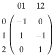
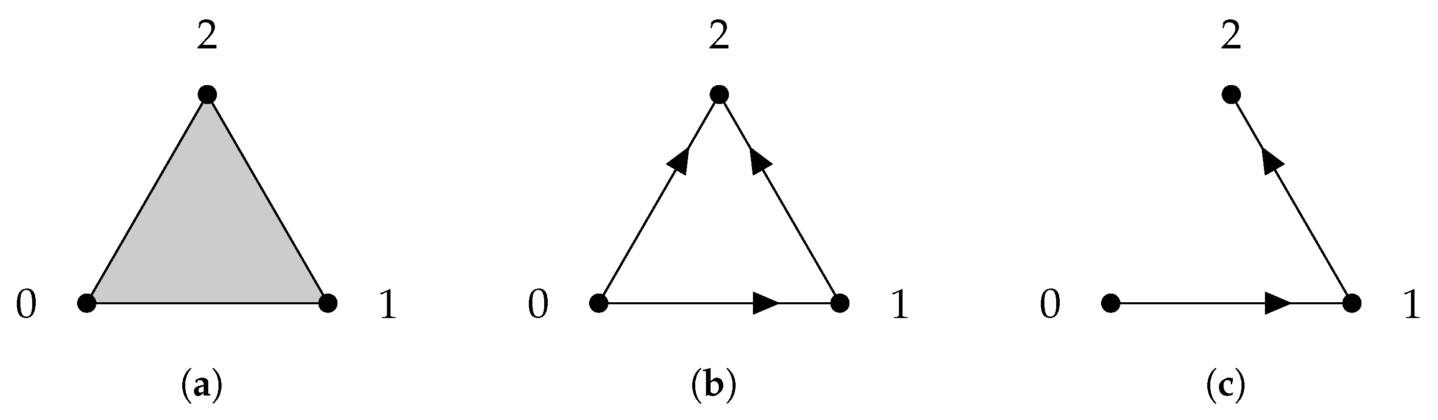
Given a finite set V, a simplicial complex X is a collection of subsets of V, such that if a set is in X, then any subset of is also in X. A set that consists of elements is referred to as a q-simplex. If is a subset of , then we say that is a face of and denote it by . The definition of a simplicial complex may seem abstract, but it is closely related to geometry. A q-simplex can be realized as the convex hull of points in a real coordinate space, so it is possible to construct a polyhedron from a simplicial complex if the simplices are glued properly. For example, supposing X is the power set of , we can identify X with a triangle whose vertices are labeled (Figure 1a). However, many geometrical objects can be sliced properly so as to give rise to a simplicial complex. We always designate a fixed order of vertices in a simplicial complex (the choice of ordering will not affect the resulting homology groups [77]) and require that the vertices of any simplices should be ordered according to the fixed ordering. For example, suppose that we use the natural ordering for the simplicial complex (Figure 1b), then we must not write the simplex as . To emphasize that a simplex is ordered, we will use the notation or .

Figure 1.
(a) The simplicial complex . (b) The simplicial complex . Arrows emphasize that vertices are ordered. (c) The simplicial complex .
We now introduce a more abstract definition. A simplicial complex X gives rise to a sequence of vector spaces and linear maps, collectively referred to as a simplicial chain complex
The chain group is the real vector space generated by q-simplices, and the boundary operator is a linear map such that
where the symbol means that is deleted. An element of is called a q-chain and, by definition, is a linear combination of q-simplices. Sometimes, it is intuitive to regard a q-chain as a function mapping a q-simplex to its coefficient. The coefficients ensure that , so the q-th homology group is well-defined. The dimension of the homology group is referred to as the q-th Betti number, which is often described as counting the number of q-dimensional “holes” in a simplicial complex. It is not always clear what a high-dimensional hole represents in a simplicial complex; nevertheless, the main idea is that homology groups extract quantitative topological information about a simplicial complex.
Example 1.
The simplicial complex (Figure 1b) has only two chain groups, and , and one boundary map , represented by the matrix
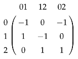 if we identify any real-valued function with the column vector , and any real valued function with the column vector . We can see that if and only if , and . Since , the homology group is and implies .
For the simplicial complex (Figure 1c), the matrix representation of is
 and we can verify that the only that satisfies is the zero function. The intuition behind the difference between and is that in X the edges constitute a close path, while in Y there are no close paths.
A simplicial chain complex is an example of a chain complex. The reader only needs to konw that a chain complex is a sequence of vector spaces and linear morphisms
where . We often assume that each is a finite-dimensional inner product space.
2.2. Combinatorial Laplacians
Many simplicial complexes share the same Betti numbers. In this case, we can resort to a class of finer descriptors called combinatorial Laplacians to distinguish among different simplicial complexes. Before we define combinatorial Laplacians, we first need to equip a chain group with an inner product. The canonical approach is to let the set of q-simplices be an orthonormal basis for the q-th chain group . Now we can discuss the adjoint of the boundary operator , denoted by , and the q-th combinatorial Laplacian [28] is defined by
When , since , the 0-th combinatorial Laplacian is just . The q-th combinatorial Laplacian is a positive semi-definite symmetric operator and only has non-negative eigenvalues. One fact of linear algebra is that, if and W are inner product spaces and , are two linear morphisms such that , then . Therefore, the kernel of the q-th combinatorial Laplacian is isomorphic to the q-th homology group [28]. This property guarantees that we can calculate Betti numbers from the spectra of combinatorial Laplacians. We can further show that admits a Hodge decomposition (a detailed exposition can be found in [33])
Example 2.
For a simple graph , let be a function that maps every vertex to a real number. If we view the simple graph as a simplicial complex, then maps to a real valued function whose domain is E. The Dirichlet energy of
measures how varies over V. Any is a function with zero Dirichlet energy. In a connected graph, if has zero Dirichlet energy, then for any two vertices a and b ( is a constant function), because there is always a path that starts from a and ends at b. If a graph has more than one connected components, only needs to be constant on any connected components. In other words, the dimension of is equal to the number of connected subgraphs.
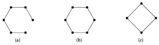
The operator is more commonly known as the graph Laplacian, and there is extensive research studying the relationship between the spectrum of a graph Laplacian and properties of a graph [25]. For a connected graph, it is well known that the minimal nonzero eigenvalue of its graph Laplacian reflects the graph’s connectivity [78]. Graphs that share the same homology groups may have different graph Laplacians (Figure 2).
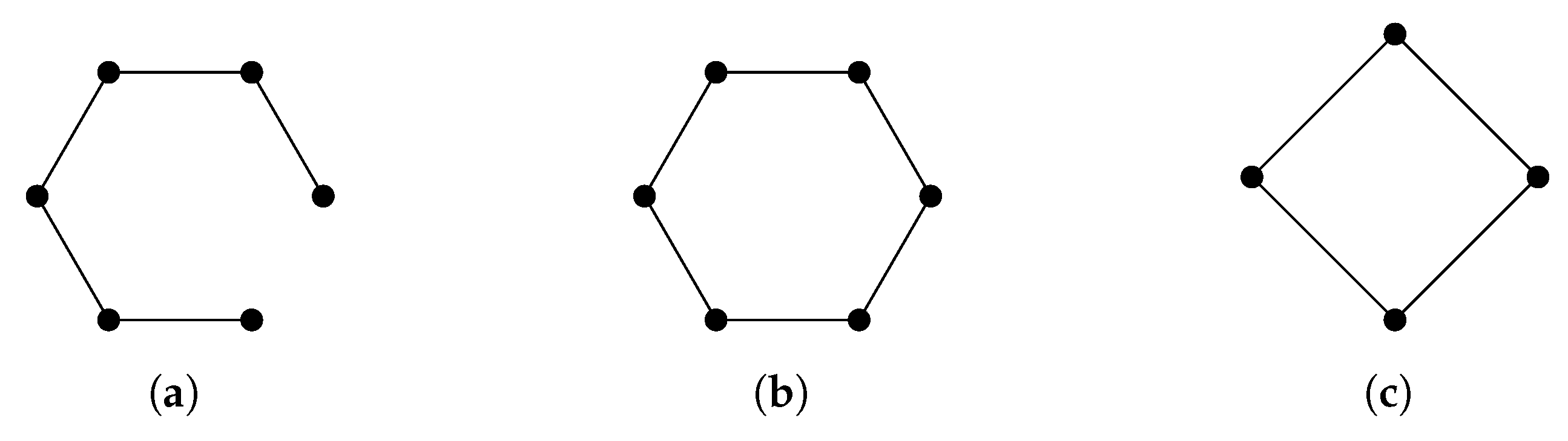
Figure 2.
Homology can distinguish (a) from (b,c), but cannot distinguish between (b,c). Laplacians can distinguish among all of them. For a cycle graph with n vertices, the spectrum of the graph Laplacian is .
2.3. Filtration and Persistent Homology
So far we have introduced the elementary theory of simplicial complexes, but we have not explained how it is related to point-cloud data. A point cloud is a set of finitely many points in a Euclidean space. Usually the geometrical structure of a point cloud is related to some non-geometrical properties of the object the point cloud represents, and a good understanding of the “geometry” of the point cloud is important. Here, the first problem is what we mean by “geometry”. A naive notion of “geometry” is the pairwise distances between each pair of points, and we can represent this information by a filtration, such that we obtain a nested sequence of simplicial complexes. One commonly used filtration is Vietoris–Rips filtration: given a point cloud and a parameter , is a simplicial complex such that the simplex if and only if the Euclidean distance between and is at most d for any . Using d, we obtain finitely many distinct simplicial complexes, each of which characterizes the shape of the point cloud on a different scale. The homology groups or combinatorial Laplacians of each will change as d varies, providing a characterization of the point cloud.
Example 3.
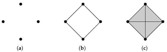
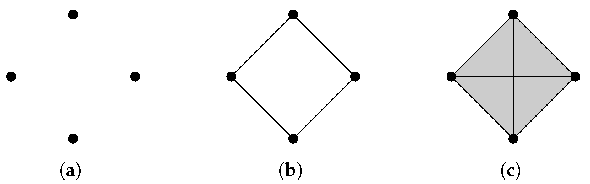
Now we build a Vietoris-Rips filtration from the point cloud shown in Figure 3a. When , there are no edges in . When , changes for the first time and becomes . If d goes from to 2, . As d becomes bigger, contains more and more simplices. Let us examine for . as there is no close path, and because of four newly born edges. When , since the close path is filled by high-dimensional simplices.
Figure 3.
(a) . (b) . (c) .
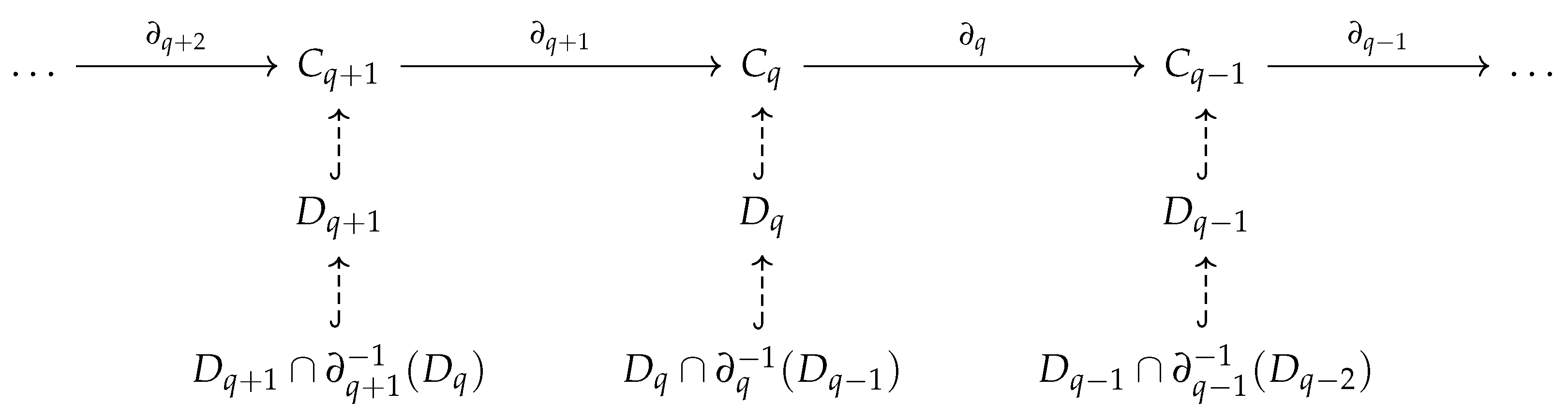
In addition to calculating homology groups or combinatorial Laplacians for each in a filtration, we can also calculate the persistent homology to quantify how topological features of a smaller complex persist in . Suppose X and Y are two simplicial complexes and , then we have the following diagram (dashed arrows indicates inclusion maps ):
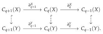 Since is larger than , some q-dimensional “holes” in X might be filled because of . The q-dimensional “holes” in X that persists in Y are , but since is not necessarily a subspace of , the proper expression should be
A more formal understanding of persistent homology is helpful. We notice that . In plain words, this means that the boundary of a simplex is unchanged if we view it as a simplex in Y. In general, for two chain complexes and , the collection of maps such that for all q is called a chain map. A chain map f induces a homomorphism , and sometimes the image is called the persistent homology group of the chain map .
3. Persistent (Combinatorial) Laplacians
3.1. Persistent Laplacians
We have shown that the kernel of the q-th combinatorial Laplacian is isomorphic to the q-th homology group. This result has been generalized for persistent homology groups.
 Given two complexes , let be the subspace
Example 4.
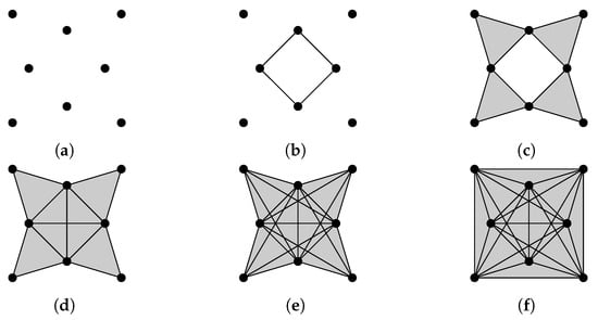
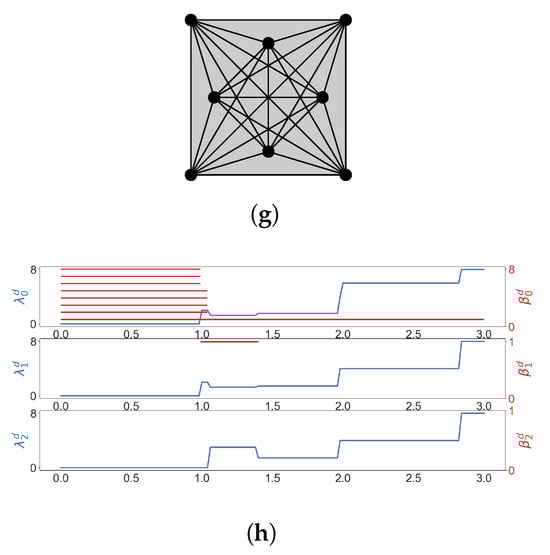
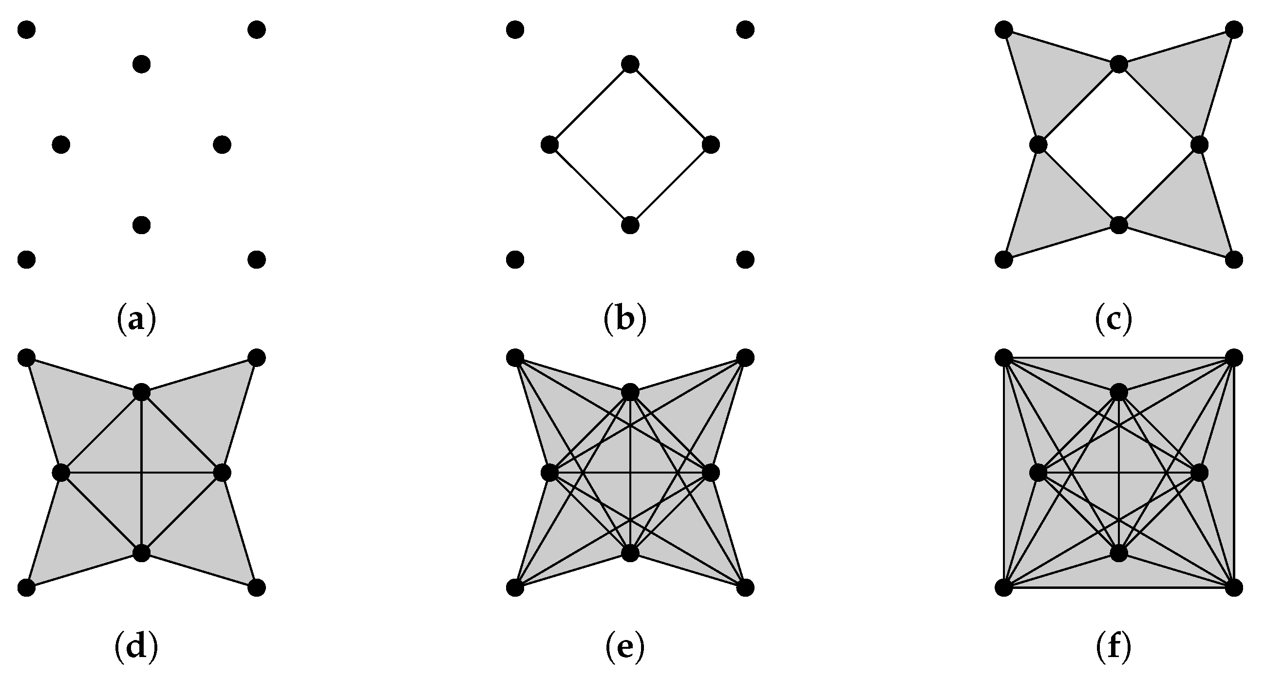
We illustrate the Vietoris–Rips filtration of a point cloud in Figure 4. Some results of Laplacian calculation are shown in Figure 4h, where d is the diameter (stepsize is 0.02), is the minimal nonzero eigenvalue of the q-th combinatorial Laplacian of , and red bars represent homology classes that persist over d. The minimal nonzero eigenvalues change at different d, indicating the formation of new simplices.
Figure 4.
The Vietoris-Rips filtration of a point cloud, and some results of Laplacian calculation. (a) ; (b) ; (c) ; (d) ; (e) ; (f) ; (g) ; (h) The horizontal axis represents the diameter d (stepsize is 0.02). (shown in blue lines) is the minimal nonzero eigenvalue of the q-th combinatorial Laplacian of , and red bars represent homology classes that persist over d.
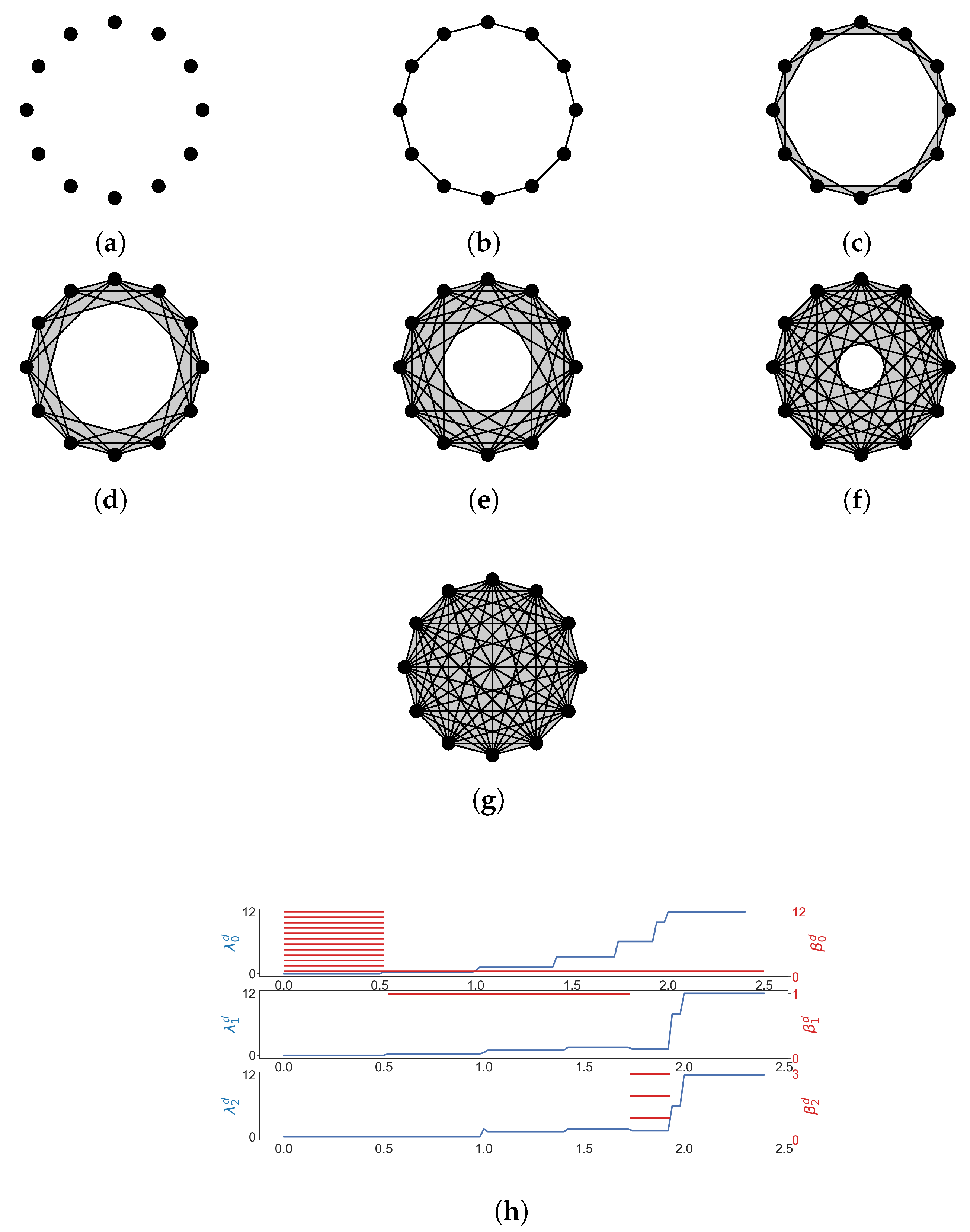
Example 5.
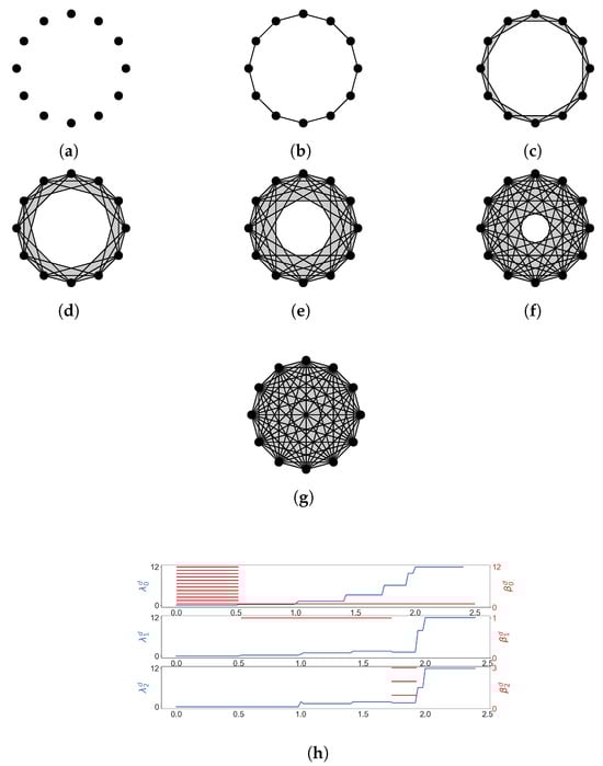
We consider the Vietoris–Rips filtration of the 12 vertices of the regular 12-gon (Figure 5). We see that goes up before any homology class is born, which means that 2-simplices form but no 2-dimensional holes are born yet. This phenomenon can be observed in many results of [63].
Figure 5.
The Vietoris-Rips filtration of the vertices of a regular 12-gon, and some results of Laplacian calculation. (a) ; (b) ; (c) ; (d) ; (e) ; (f) ; (g) ; (h) The horizontal axis represents the diameter d (stepsize is 0.02). (shown in blue lines) is the minimal nonzero eigenvalue of the q-th combinatorial Laplacian of , and red bars represent homology classes that persist over d.
3.2. Matrix Representations of a (Persistent) Laplacian
Since has a canonical orthonormal basis, the matrix representation of is the transpose of the matrix representation of . In the computation of persistent Laplacians, the difficult part is the calculation of the upper persistent Laplacian, because we need to determine , which may not have a canonical orthonormal basis. We can obtain a basis of by performing a column reduction for or by directly calculating the matrix representation of the upper persistent Laplacian by Schur complement [56]. We give two examples in the following.
Example 6.
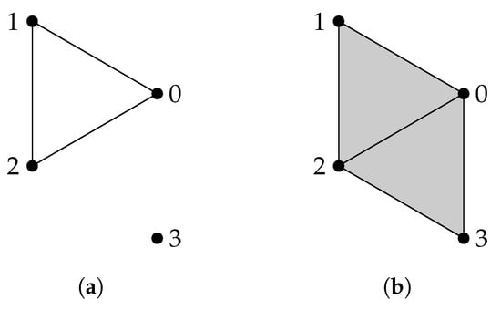
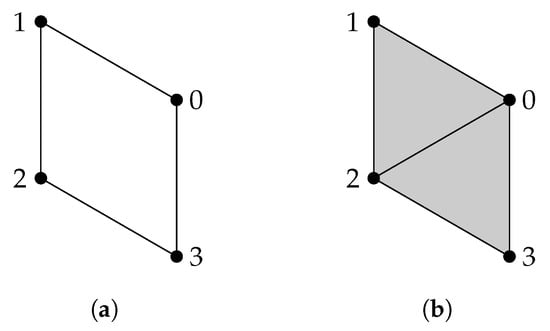
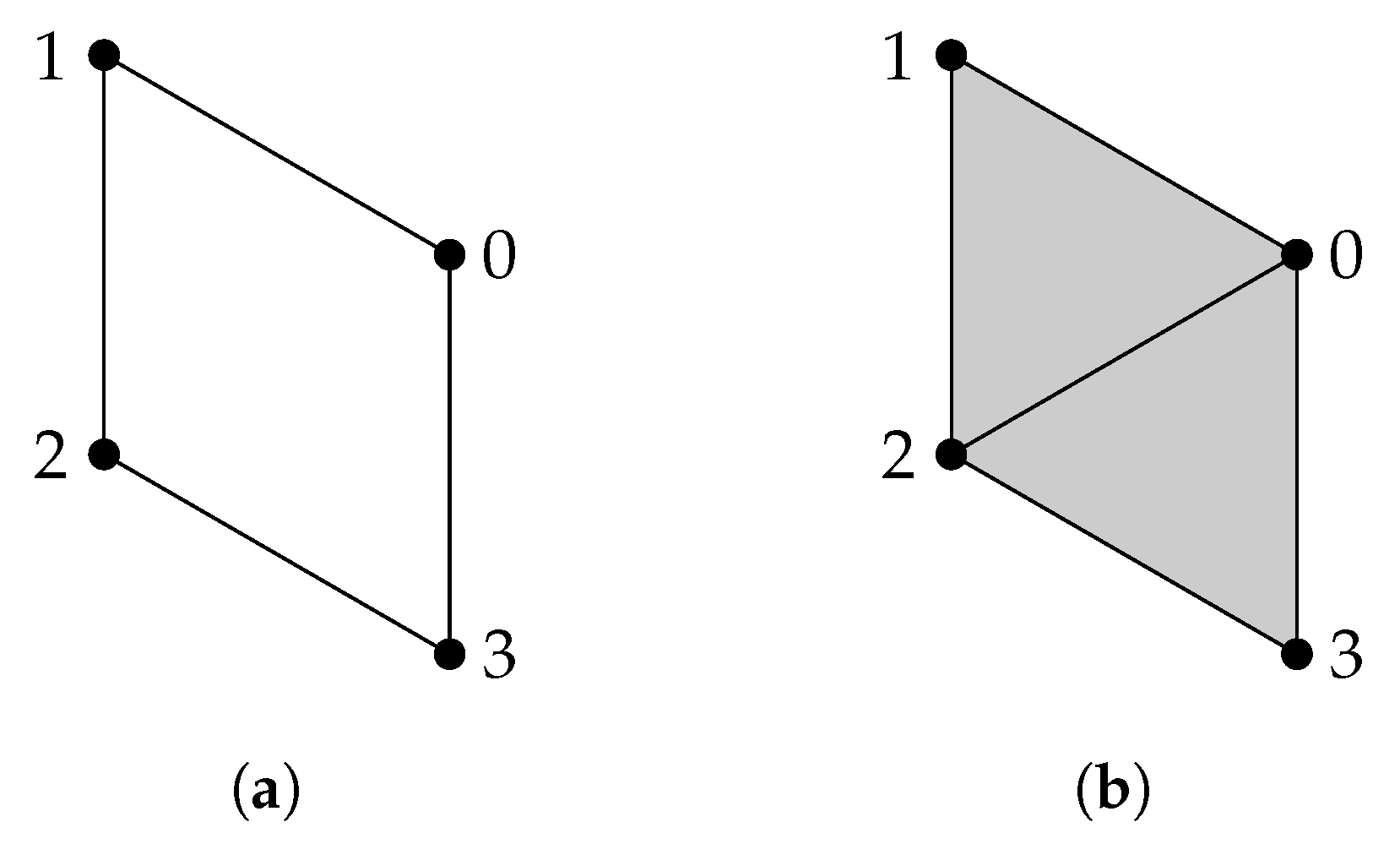
When is generated by some -simplices in Y, the calculation of is relatively easy. For X and Y shown in Figure 6, we compute . The matrix representation of is
 so is generated by 012; then, the matrix representation of is
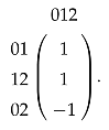
Figure 6.
(a) and (b) .
Example 7.
We compute for X and Y shown in Figure 7.
Figure 7.
(a) and (b) .
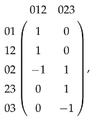
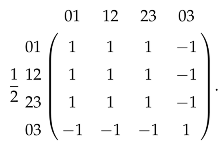
The matrix representation of is
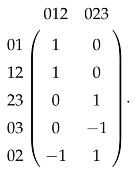 Our goal is to make the submatrix
in column echelon form. We apply one column reduction and obtain
Our goal is to make the submatrix
in column echelon form. We apply one column reduction and obtain
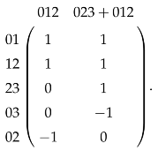 Therefore, and one matrix representation of is
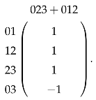
For any two spaces V and W and , if we choose arbitrary bases of V and W and take a matrix representation of f, then the matrix representation of is , where P and Q are inner product matrices of V and W, respectively. If we use as the basis of , then the inner product matrix of is 2 (the norm of ). The corresponding matrix representation of is
and the matrix representation of the upper persistent Laplacian is
 Another way to compute the upper persistent Laplacian is as follows. We first compute the upper Laplacian
 then treat this matrix as a block matrix
 and compute the Schur complement .
3.3. Eigenvectors of a Laplacian
There are some results concerning the relationship between the spectra of Laplacians and the shape of a simplicial complex [26,79]. How do we interpret the eigenvectors of a Laplacian? For an eigenvector of a q-th combinatorial Laplacian, we can look at the shape of q-simplices where the eigenvector has support (signs are arbitrary because they are affected by the fixed ordering of vertices). Empirical observations [80,81,82] suggest that (a) harmonic eigenvectors (eigenvectors of zero eigenvalues) have support near q-dimensional “holes” (or vertices in a connected component when ) or (b) nonharmonic eigenvectors (eigenvectors of nonzero eigenvalues) have support near “clusters” of q-simplices. In terms of persistent Laplacians, very little is known about the topological interpretation of eigenvalues and eigenvectors.
4. Generalizations of (Persistent) Laplacians
From a theoretical point of view, it is natural to ask whether a persistent Laplacian can be defined in other settings such that the persistent Hodge theorem still holds. From a practical point of view, generalizations of persistent Laplacians are motivated by the need to integrate non-geometrical data that are important for specific problems. In the next few sections, we will introduce structures such as cellular (co)sheaves, digraphs, and hyper(di)graphs, and then review some recent advances in their homology and Laplacians. We will also discuss Dirac operators and N-chain complexes at the end of this section.
4.1. Differential Graded Inner Product Spaces
It has been noted earlier that persistent Laplacians can be defined analogously for differential graded inner product spaces and the persistent Hodge theorem can be proved. A differential graded inner product space is just a chain complex
whose chain groups are inner product spaces. When we say is a subspace of , we mean that the inner space structure and boundary operator of are inherited from . For a pair of differential graded inner product spaces , the q-th persistent homology group is defined analogously by
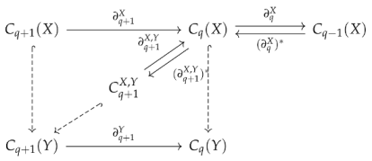
Observe that . The preimage of under is just . Hence, is the image of , where is the projection map from W to V. We denote by , and by . These maps are shown in the following diagram:
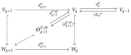 where hooked dashed arrows represent inclusion maps. We define the q-th persistent Laplacian by
4.2. Persistent Laplacians for Simplicial Maps
The classical filtration of simplicial complexes only represents one type of shape evolution. We also need tools to study more general shape evolution, such as the sparsification of a simplicial complex. This requires us to consider general simplicial maps rather than inclusion maps. Gülen et al. [54] developed a theory of persistent Laplacians for a simplicial map. Suppose is a simplicial map
 where is induced by f. Different from the original q-th persistent Laplacian for an inclusion map, we need to define two subspaces
4.3. Weighted Simplicial Complexes
A simplicial complex whose simplices have weights is generally called a weighted simplicial complex. The weights can be geometrical, such as angles between simplices, volumes of simplices, or non-geometrical such as numbers of scientific papers coauthored by groups of people. Many theories and models involving weighted simplicial complexes exist (e.g., [83,84,85,86,87,88]). Here, we focus on the theory of weighted simplicial complexes proposed by Dawson [89] and later developed in [90,91,92,93,94,95,96]. A weighted simplicial complex is a simplicial complex where each simplex has a weight valued in a commutative ring R, such that if , then is divisible by . The weighted chain complex of a weighted simplicial complex X is defined as follows. Let be the set of formal sums of q-simplices with coefficients in R (if is zero, then we do not include in any formal sum). For , we denote the face by . The weighted boundary operator ∂ is given by
As is divisible by , the weighted boundary operator is well defined. We still have , because for ,
Therefore, weighted homology groups can be defined analogously. Wu et al. [95] pointed out that in the proof of , what really matters is the quotient of weights. If we write as , then the equality
becomes
which means that any satisfying this equality induces a (-weighted) boundary operator
A simplicial complex paired with a generalized weight function is called a -weighted simplicial complex.
Example 8
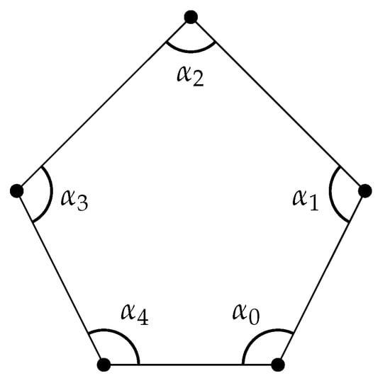
([95]). A weighted polygon is a polygon with (Figure 8).
Figure 8.
A weighted polygon.
The matrix representation of is
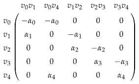 and the resulting weighted is dependent on . The weighted homology of weighted polygons might be useful for analyzing ring structures in biomolecules.
We have emphasized that a point cloud can be studied by building a filtration of simplicial complexes. If we want to distinguish some points from other points, we can assign weights and building a filtration of weighted simplicial complexes [94]. We may also consider weighted versions of (persistent) Laplacians [95].
Example 9.
Suppose each point v in a point cloud has weight . We can associate any simplex as the product weight [94]
Since the weighted boundary map can be given by
We can just define the q-th chain group as the space generated by q-simplices without worrying about zero weights.
Example 10.

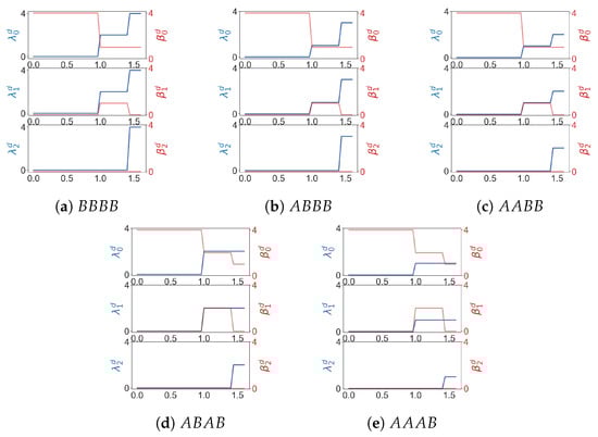
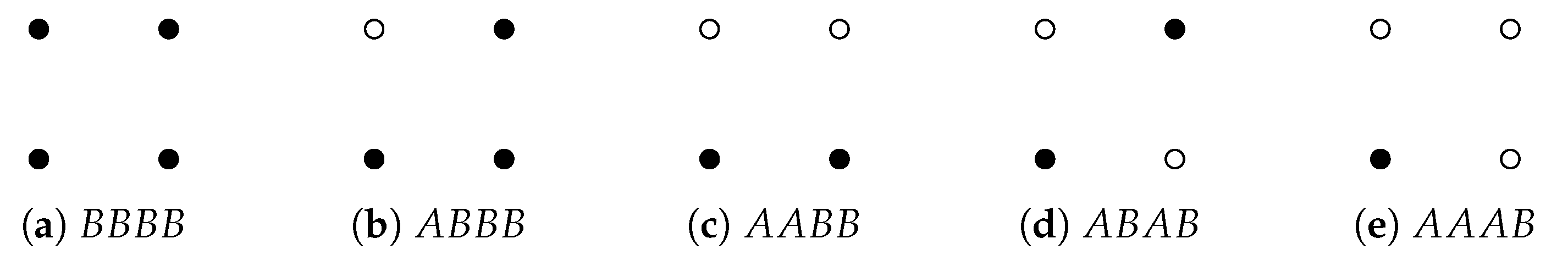
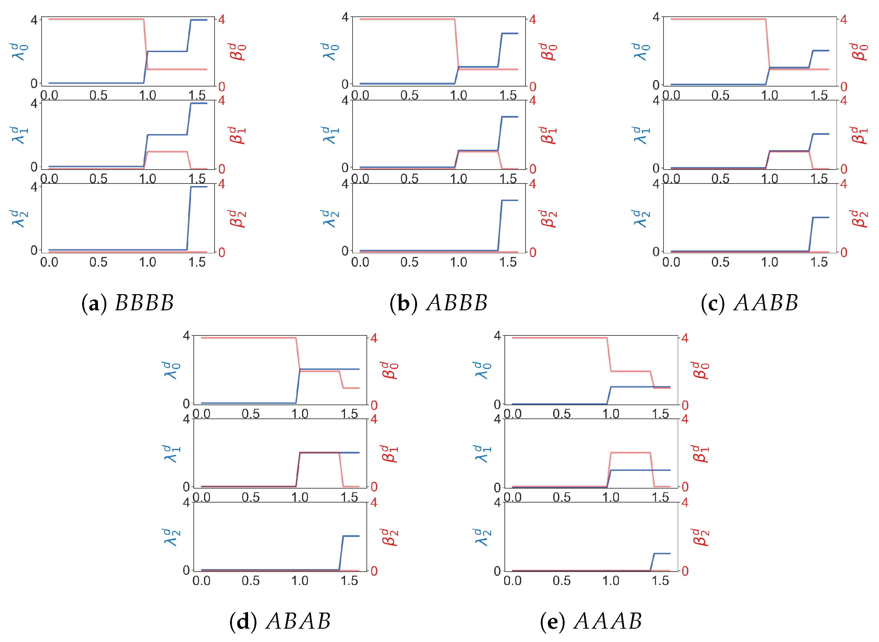
Suppose a point cloud contains two types of points A and B. We can assign weights to , and compute weighted homology and Laplacians using product weighting. At least when a point cloud is simple, weighted combinatorial Laplacians can be used to differentiate among different patterns of distribution of A and B. For a point cloud of four points there are five configurations (shown in Figure 9) that include at least one point whose weight is 1. Results of weighted Laplacians are shown in Figure 10.
Figure 9.
Five configurations of A and B.
Figure 10.
is the minimal nonzero eigenvalue of the q-th weighted combinatorial Laplacian for in a Rips filtration. is the q-th Betti number of .
4.4. Cellular (Co)Sheaves
In a -weighted simplicial complex, we can imagine that a copy of R resides on each simplex and is a scalar multiplication from the copy on to the copy on [97]. If we associate each simplex with a vector space and designate a linear morphism for every face relation, we will obtain cellular (co)sheaf. The theory of cellular (co)sheaves was first introduced in [98] and later gained attention for its application potential (e.g., [99,100,101,102,103]). In recent years, the study of sheaf neural networks has become a trending topic [104,105,106,107]. Like a weighted simplicial complex, a cellular (co)sheaf is a candidate for modeling complex objects such as molecules.
A cellular cosheaf is a simplicial complex X with additional data (for ease of exposition, we have simplified the definition of a cellular (co)sheaf). Each simplex is assigned a vector space (or denoted by ), called the stalk over , and for any face relation , there is an extension map (or denoted by ). The q-th chain group of a cellular cosheaf is the direct sum of stalks over q-simplices and the boundary map ∂ is given by
The square of this boundary map is 0, if for any face relation we have
A dual concept is a cellular sheaf. For a cellular sheaf , is a map from to (called a restriction map). An analogous sheaf cochain complex can be defined. If stalks are inner product spaces, one can equip inner product structures for (co)chain groups. Applying the construction of combinatorial Laplacians to a cosheaf chain complex or a sheaf cochain complex, we obtain (co)sheaf Laplacians [97]. It is noted that many sheaves over a digraph only have trivial 0-dimensional cohomology groups [108], but we can still extract some information from sheaf Laplacians.
Example 11.
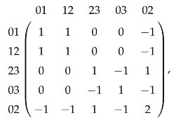
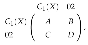
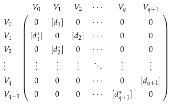
Suppose there is a sheaf over the simplicial complex , then the sheaf coboundary map is represented by the block matrix
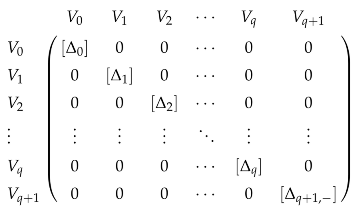
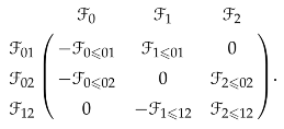 Suppose all stalks are inner product spaces and they are orthogonal to each other, then the 0-th sheaf Laplacian is represented by the block matrix
Persistent (co)sheaf (co)homology is known by experts [109,110], and a systematic treatment can be found in [111]. One type of filtration of sheaves is as follows. A sheaf on X is a “subsheaf” of over Y if and the stalks and restriction maps of are the same as those of . To define the q-th persistent sheaf Laplacian [59] for , we can first endow chain groups with inner product structures and dualize everything to make and cosheaves, such that there is an inclusion chain map between their cosheaf chain complexes. Then, we can define the q-th persistent sheaf Laplacian as the q-th persistent Laplacian of the cosheaf chain complexes.
4.5. Path Homology, Flag Homology, and Digraphs
The motivation behind path homology is to construct a homology theory of digraphs such that directional information of edges is encoded and higher-dimensional homology groups are non-trivial. Path homology (there are other (co)homology theories of digraphs [112,113,114,115]) was proposed by Grigor’yan, Lin, Muranov, and Yau [116] and developed in various papers [117,118,119,120,121]. A summary of recent advances in path homology of digraphs can be found in [122]. Recall that a digraph (without self-loops) is a pair where E is a set of ordered pairs of vertices. An allowed q-path is an ordered finite sequence of vertices such that for all . If we take the space generated by allowed p-paths (denoted by ) as the q-th chain group, and define the boundary map by
then formally we can show that . However, may include paths that are not allowed. To solve this problem, we first need to introduce some general concepts.
Definition 1.
Suppose X is a finite set. An elementary p-path is a sequence of elements of X. The space generated by all elementary p-paths with coefficient in is denoted by . The q-th non-regular boundary map is given by
We can prove that this is a chain complex. Among all paths, a path that lingers at a vertex (for some i, ) is considered a degenerate path, since we are not interested in self-loops.
Definition 2.
A path over X where for each i is called regular. The space generated by all regular q-paths is denoted by .
We define a new boundary operator between regular paths. When computing , we first compute and treat all irregular paths arising from it as zeros. We can still verify that [123].
Now, given a digraph , every is a subspace of .
One way to make well-defined is to restrict to the subspace . We have to verify that . is true by definition and is true since . Therefore, we have the chain complex
and the definition of a path homology group is straightforward. The q-th chain group is called the space of ∂-invariant q-paths on G, denoted by (if a digraph is not simple, there will be two choices of [116] that might be suitable for different problems [124]). Regarding the geometrical interpretation of path homology, we only know that non-reduced is the number of connected components of the underlying undirected graph. Chowdhury et al. [125] obtained some characterizations of path homologies of certain families of small digraphs. Since edge direction information is encoded in path homology, path homology can be used to distinguish network motifs [126] and isomers in molecular and materials sciences [127]. We can also quantify the importance of a node in a network by observing changes in path homology when the node is removed [127].
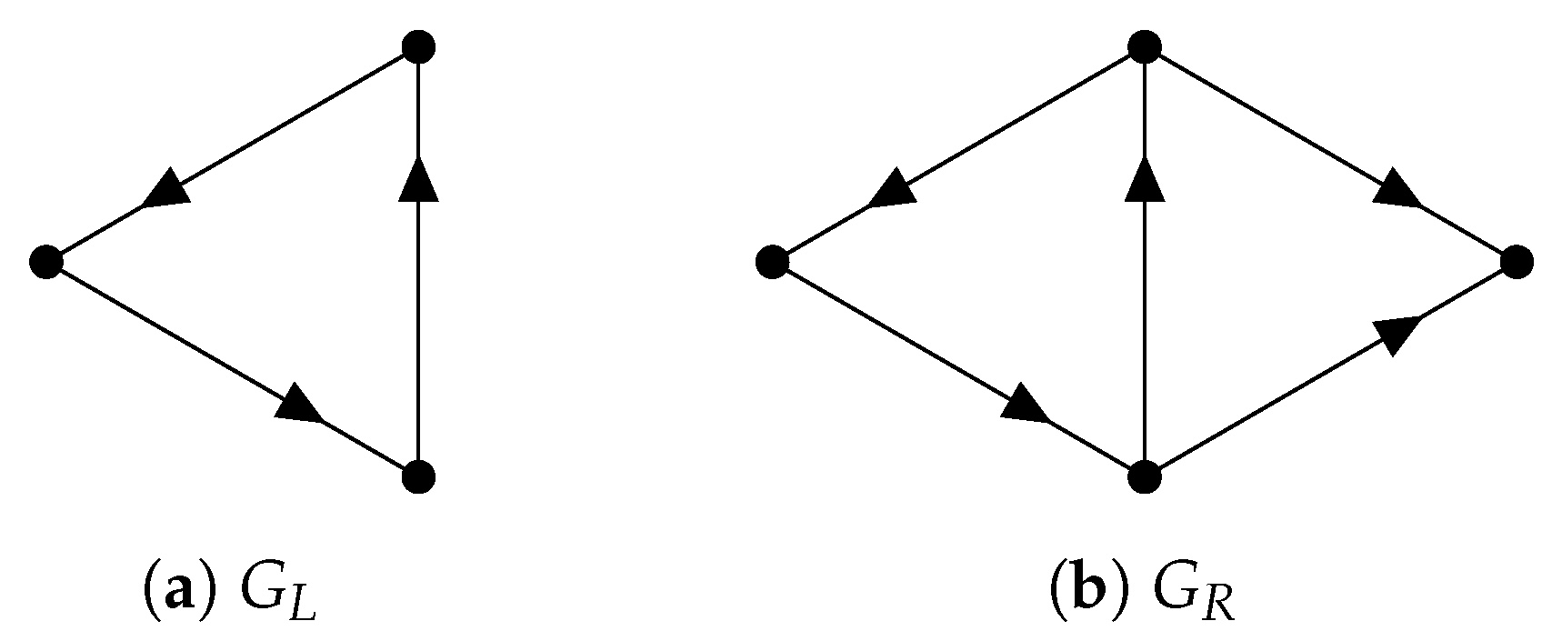
Since inherits the inner product structure from , the so-called path Laplacians (another type of path Laplacians was proposed by Estrada [128] and applied in molecular biology [129]) can be defined. We can use path Laplacians [58,122,130] to distinguish among digraphs that have the same path homology. For example, according to ([116], Theorem 5.4), the following two digraphs and (see Figure 11) have the same path homology. However, the spectrum of the 0-th path Laplacian of is and that of is .
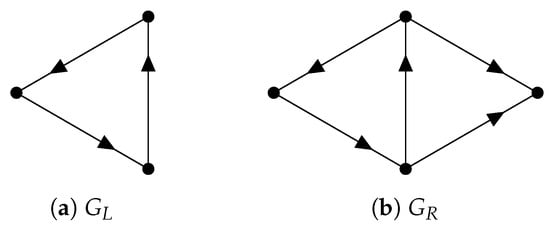
Figure 11.
Two digraphs that have the same path homology.
Persistent path homology was proposed by Chowdhury and Mémoli [126] to study a digraph where each edge e has a weight . A filtration of digraphs is constructed so that if and only if . Wang and Wei [58] introduced persistent path Laplacians and demonstrated that persistent path Laplacians can be applied to the study of molecules, since much information about molecules can be encoded in digraphs.
Flag complexes, also known as clique complexes, are another way to construct homology for digraphs, and they arise naturally in many situations [113]. Jones and Wei [57] introduced persistent directed flag Laplacians as a distinct way of analyzing flag complexes and applied them to analyze protein–ligand binding data.
Example 12.
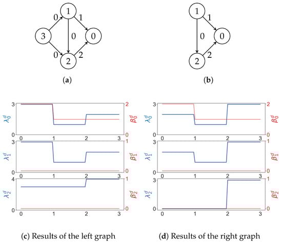
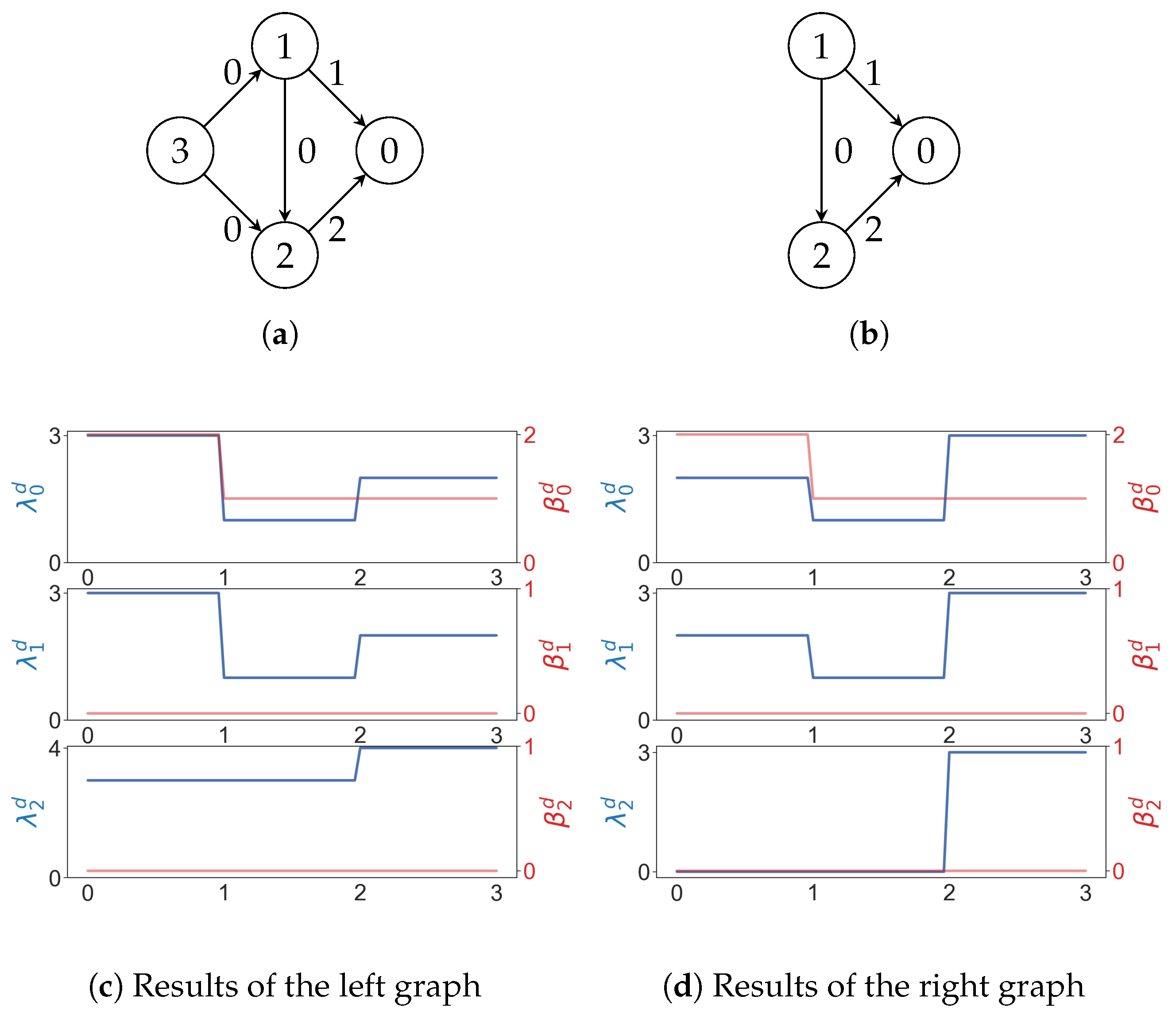
For a weighted digraph, we can build a filtration such that iff . Two weighted graphs whose path Betti numbers are the same for every may have different path Laplacians (Figure 12).
Figure 12.
In (a,b), numbers on edges are weights. In (c,d), the x axis represents the weight. As usual, and represent the minimal nonzero eigenvalues and Betti numbers.
4.6. Hypergraphs and Hyperdigraphs
A hypergraph H is a pair where E is a subset of the power set of V. An element consisting of elements is called a q-hyperedge. To define a chain complex for hypergraphs, the problem is identical to what we encounter in path homology. If we define the q-th chain group as the vector space generated by q-hyperedges, the boundary map is not well defined. One solution is to consider associated simplicial complex (simplicial closure) of a hypergraph [131], that is, the minimal simplicial complex that contains a hypergraph. Another solution inspired by path homology is embedded homology [132]. If we examine the chain complex of the associated simplicial complex, each simplicial chain group contains , the vector space generated by q-hyperedges. We only need to restrict the domain of the simplicial boundary operator to
and then the boundary operator is well-defined (Figure 13).

Figure 13.
How to costruct embedded homology.
A hyperdigraph is a hypergraph in which each hyperedge is ordered (there are other definitions of a hyperdigraph [133,134]), and its embedded homology can be defined analogously [61]. The persistent homology of hypergraphs and hyperdigraphs was studied in [132,135,136]. Persistent hypergraph Laplacians were proposed by Liu et al. [60] and persistent hyperdigraph Laplacians were introduced by Chen et al. [61] Alternative approaches to the homology and Laplacians of hypergraphs include [137,138,139,140,141,142].
4.7. Persistent Dirac Operators
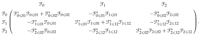
In addition to Laplacians, Dirac operators on chain complexes have also been studied [143,144,145,146,147,148]. Given a chain complex
where each chain group is a finite-dimensional inner product space, the q-th Dirac operator is represented by the block matrix
 where denotes a matrix representation of a linear morphism. Dirac operators are closely related to combinatorial Laplacians. If we think of all combinatorial Laplacians as a single operator on V, then the q-th Dirac operator is the restriction of the square root on . We can also see this by direct computation. The square of is
 where is the q-th combinatorial Laplacian. Hence, the square of any eigenvalue of a Dirac operator must be an eigenvalue of a combinatorial Laplacian.
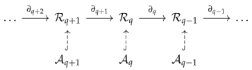
Recall that when we define persistent Laplacians, we construct an auxiliary subspace of and a map . Since is actually a subspace of , all and constitute an auxiliary chain complex
The q-th persistent Dirac operator of simplicial complexes is just the q-th Dirac operator in this auxiliary complex. The square of a persistent Dirac operator is not necessarily a block matrix consisting of persistent Laplacians. It is also possible to extend persistent Dirac operators to other settings, such as path complexes and hypergraphs [146].
4.8. Mayer Homology
In classical homology theory, the square of the boundary operator d of a chain complex must be zero (). However, this constraint can be relaxed in the so-called Mayer homology theory using an N-chain complex [72]. An N-chain complex is a sequence of abelian groups and group morphisms where . In fact, a simplicial complex can give rise to an N-chain complex. Recall that in a simplicial chain complex, the boundary operator is given by
For a prime number N, let , and we can define a generalized boundary operator d by
and prove that . Although the N-chain complex is not a chain complex in general, observe that for any positive integer
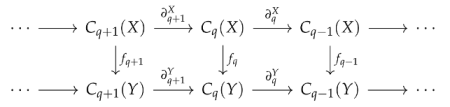
resembles a part of chain complex. We can define the Mayer homology group [72] and Mayer Laplacians (which can be thought of as ) analogously [73]. When , an N-chain complex reduces to a chain complex, and a Mayer homology group reduces to a normal homology group. Shen et al. [73] also introduced persistent Mayer homology and persistent Mayer Laplacians on N-chain complexes. Suppose , then we have the following commutative diagram
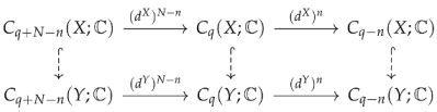 and persistent Mayer Laplacians can be defined analogously. Compared to simplicial homology, Mayer homology and Mayer Laplacians provide more features since we can vary parameters N and n. Mayer homology and the Mayer Laplacians also concern a general relationship between different dimensions. Persistent Mayer homology has been applied to protein–ligand binding affinity predictions [149].
5. Conclusions and Outlook
5.1. Persistent Topological Laplacians Versus Topological Data Analysis
The development of persistent topological Laplacians (PTLs) was driven by the need to address the limitations of persistent homology in the modeling of complex biomolecular data [24,52]. The kernels of persistent Laplacians have been shown to be isomorphic to their corresponding persistent homology groups, indicating that the information encoded in barcodes is also reflected in the spectra of persistent Laplacians [24,55,56]. Similar theoretical results apply to various PTLs designed for specific data types. The techniques outlined in this survey provide a framework for transforming point clouds or networks into algebraic features that capture both spatial and non-spatial information. These low-dimensional features have proven to be effective in supervised and unsupervised machine learning, uncovering hidden patterns, and demonstrating advantages over classical TDA methods in practical applications [70,71].
Broadly, while traditional TDA has focused predominantly on homology theory, PTLs mark a significant expansion of TDA into spectral theory. Moreover, recent advances, such as the introduction of persistent Dirac operators for flag complexes, digraphs, and hyperdigraphs, open new avenues of exploration [143,144,145,146,147,148].
The continued extension of TDA into areas such as spectral theory, geometric topology (e.g., persistent Jones polynomial [150] and persistent Khovanov homology [151]), and differential geometry (e.g., persistent de Rham–Hodge theory [52] and persistent Hodge Laplacians [53]) highlights its growing versatility. These developments promise to drive transformative progress in both theoretical research and real-world applications, enhancing the utility of TDA across a wide range of disciplines.
5.2. Limitations of Persistent Topological Laplacians
Although persistent topological Laplacians (PTLs) offer significant potential, it is important for researchers to recognize their limitations. The diversity of PTLs, when applied to point clouds [24], differentiable manifolds [52], or 1D curves embedded in higher dimensions [151,152], presents challenges in understanding the intricate relationship between the geometry and topology of the data and the PLT spectra. A deeper understanding of these relationships is essential for the successful and meaningful application of PTLs to real-world problems.
Despite advances in computational algorithms and software development [56,62,63], the computation of PTLs remains computationally intensive, especially for large datasets. Given that the primary strength of topological data analysis (TDA) lies in addressing complex challenges in data science, the development of efficient and robust PTL software packages is among the most pressing needs for advancing the field. Furthermore, the creation of finite field PTLs holds great promise for broadening the applicability of PTLs in data science and beyond.
5.3. Future Works
The field of PTLs is dynamic and rapidly evolving. The future development of PTLs is wide open, and we envision the exploration of the following topics:
(1) To some extent, the success of TDA can be attributed to its integration with machine learning, particularly with the first introduction of topological deep learning in 2017 [11]. Sheaf neural networks [107], sheaf attention [104], and neural sheaf diffusion [105] are popular topics. Similarly, the development of efficient PTL representations for machine learning, including deep learning, is also an important topic. The featurization of Laplacians typically requires domain knowledge and experience. Since self-learning representations of persistent diagrams have been proposed [153], we wonder if self-learning representations of (persistent) Laplacians are possible. As the eigenvectors of the PTLs were found to have better descriptive power than eigenvalues [57], featurization of the PTL eigenvectors is also an interesting future topic.
(2) PTLs have been formulated on a variety of mathematical objects, including simplicial complexes, directed flag complexes, path complexes, cellular sheaves, digraphs, hypergraphs, and hyperdigraphs. One can also extend PTLs to settings such as the Hochschild complex [154], quantum homology [155], multiparameter persistent homology [156], and interaction homotopy and interaction homology [157,158]. We expect that these developments will further extend the scope and capability of the current TDA for real-world applications.
(3) It is possible that persistent sheaf Dirac operators can be devised to distinguish certain geometric shapes. Additionally, persistent Dirac operators defined on a spinor bundle may extend persistence to index theory, such as multiscale index theory.
(4) The PTLs on manifolds, such as the evolutionary de Rham–Hodge theory, pose implementation challenges compared to their discrete counterparts on point clouds [34]. Recently, the persistent de Rham–Hodge Laplacian in Eulerian representation has been proposed for manifold topological learning (MTL) [53]. Persistent de Rham–Hodge Laplacians extend earlier persistent homology in the cubical setting [159,160,161]. From a theoretical point of view, it will be interesting to extend various PTLs to the setting of manifolds (with boundaries).
(5) In addition to point cloud data and data in manifolds, there are knot-type data, such as DNA packaging in Hi-C data and entangled brain neurons. Knots are traditionally studied with invariants, such as the Alexander polynomial, the Jones polynomial, and the Kauffman polynomial [162]. Song et al. proposed the multiscale Jones polynomial and the persistent Jones polynomial [150]. Khovanov homology [163] is a major breakthrough in knot theory. Shen et al. [151] proposed an evolutionary Khovanov homology for weighted links. Jones and Wei [152] proposed Khovanov Laplacians and showed that, at least for chiral prime knots up to 10 crossings, they can distinguish chiral knots from their mirrors. Based on these developments, PTLs on knot- or curve-type data, i.e., persistent Khovanov Laplacians, can be formulated, and future research on computational geometric topology is widely open.
(6) Finally, ChatGPT ushers in a new era of artificial intelligence (AI), offering wide-ranging opportunities in all disciplines. ChatGPT and other chatbots effectively transform pure mathematical theories into practical computational tools, including PTLs [164]. Both AI-enabled topology and topology-enabled AI will have a growing impact on research [165].
Funding
This work was supported in part by NIH grant R35GM148196, National Science Foundation grants DMS2052983 and IIS-1900473, MSU Foundation, and Bristol-Myers Squibb 65109.
Data Availability Statement
The data will be made available by the authors on request.
Acknowledgments
The authors thank Fei Han, Fengchun Lei, Fengling Li, Zhi Lu, Jie Wu, and Kelin Xia for useful discussions.
Conflicts of Interest
The authors declare no conflicts of interest.
References
- Edelsbrunner, H.; Harer, J. Persistent homology—A survey. Contemp. Math. 2008, 453, 257–282. [Google Scholar]
- Zomorodian, A.; Carlsson, G. Computing persistent homology. Discret. Comput. Geom. 2005, 33, 249–274. [Google Scholar] [CrossRef]
- Ghrist, R. Barcodes: The persistent topology of data. Bull. Am. Math. Soc. 2008, 45, 61–75. [Google Scholar] [CrossRef]
- Adams, H.; Emerson, T.; Kirby, M.; Neville, R.; Peterson, C.; Shipman, P.; Chepushtanova, S.; Hanson, E.; Motta, F.; Ziegelmeier, L. Persistence images: A stable vector representation of persistent homology. J. Mach. Learn. Res. 2017, 18, 1–35. [Google Scholar]
- Xia, K.; Wei, G.W. Multidimensional persistence in biomolecular data. J. Comput. Chem. 2015, 36, 1502–1520. [Google Scholar] [CrossRef]
- Bubenik, P. Statistical topological data analysis using persistence landscapes. J. Mach. Learn. Res. 2015, 16, 77–102. [Google Scholar]
- Bae, W.; Yoo, J.; Chul Ye, J. Beyond deep residual learning for image restoration: Persistent homology-guided manifold simplification. In Proceedings of the IEEE Conference on Computer Vision and Pattern Recognition Workshops, Honolulu, HI, USA, 21–26 July 2017; pp. 145–153. [Google Scholar]
- Clough, J.R.; Byrne, N.; Oksuz, I.; Zimmer, V.A.; Schnabel, J.A.; King, A.P. A topological loss function for deep-learning based image segmentation using persistent homology. IEEE Trans. Pattern Anal. Mach. Intell. 2020, 44, 8766–8778. [Google Scholar] [CrossRef]
- Dabaghian, Y.; Mémoli, F.; Frank, L.; Carlsson, G. A topological paradigm for hippocampal spatial map formation using persistent homology. PLoS Comput. Biol. 2012, 8, e1002581. [Google Scholar] [CrossRef]
- Townsend, J.; Micucci, C.P.; Hymel, J.H.; Maroulas, V.; Vogiatzis, K.D. Representation of molecular structures with persistent homology for machine learning applications in chemistry. Nat. Commun. 2020, 11, 3230. [Google Scholar] [CrossRef]
- Cang, Z.; Wei, G.W. TopologyNet: Topology based deep convolutional and multi-task neural networks for biomolecular property predictions. PLoS Comput. Biol. 2017, 13, e1005690. [Google Scholar] [CrossRef]
- Cang, Z.; Wei, G.W. Integration of element specific persistent homology and machine learning for protein-ligand binding affinity prediction. Int. J. Numer. Methods Biomed. Eng. 2018, 34, e2914. [Google Scholar] [CrossRef] [PubMed]
- Gameiro, M.; Hiraoka, Y.; Izumi, S.; Kramar, M.; Mischaikow, K.; Nanda, V. A topological measurement of protein compressibility. Jpn. J. Ind. Appl. Math. 2015, 32, 1–17. [Google Scholar] [CrossRef]
- Kovacev-Nikolic, V.; Bubenik, P.; Nikolić, D.; Heo, G. Using persistent homology and dynamical distances to analyze protein binding. Stat. Appl. Genet. Mol. Biol. 2016, 15, 19–38. [Google Scholar] [CrossRef] [PubMed]
- Lee, Y.; Barthel, S.D.; Dłotko, P.; Moosavi, S.M.; Hess, K.; Smit, B. Quantifying similarity of pore-geometry in nanoporous materials. Nat. Commun. 2017, 8, 15396. [Google Scholar] [CrossRef]
- Xia, K.; Feng, X.; Tong, Y.; Wei, G.W. Persistent homology for the quantitative prediction of fullerene stability. J. Comput. Chem. 2015, 36, 408–422. [Google Scholar] [CrossRef]
- Jiang, Y.; Chen, D.; Chen, X.; Li, T.; Wei, G.W.; Pan, F. Topological representations of crystalline compounds for the machine-learning prediction of materials properties. Npj Comput. Mater. 2021, 7, 28. [Google Scholar] [CrossRef]
- Horak, D.; Maletić, S.; Rajković, M. Persistent homology of complex networks. J. Stat. Mech. Theory Exp. 2009, 2009, P03034. [Google Scholar] [CrossRef]
- Nguyen, D.D.; Cang, Z.; Wei, G.W. A review of mathematical representations of biomolecular data. Phys. Chem. Chem. Phys. 2020, 22, 4343–4367. [Google Scholar] [CrossRef]
- Nguyen, D.D.; Cang, Z.; Wu, K.; Wang, M.; Cao, Y.; Wei, G.W. Mathematical deep learning for pose and binding affinity prediction and ranking in D3R Grand Challenges. J. Comput.-Aided Mol. Des. 2019, 33, 71–82. [Google Scholar] [CrossRef]
- Chen, J.; Wang, R.; Wang, M.; Wei, G.W. Mutations strengthened SARS-CoV-2 infectivity. J. Mol. Biol. 2020, 432, 5212–5226. [Google Scholar] [CrossRef]
- Papamarkou, T.; Birdal, T.; Bronstein, M.M.; Carlsson, G.E.; Curry, J.; Gao, Y.; Hajij, M.; Kwitt, R.; Lio, P.; Di Lorenzo, P.; et al. Position: Topological Deep Learning is the New Frontier for Relational Learning. In Proceedings of the Forty-first International Conference on Machine Learning, Vienna, Austria, 21–27 July 2024. [Google Scholar]
- Lieutier, A. Talk: Persistent Harmonic Forms. 2014. Available online: https://project.inria.fr/gudhi/files/2014/10/Persistent-Harmonic-Forms.pdf (accessed on 11 January 2024).
- Wang, R.; Nguyen, D.D.; Wei, G.W. Persistent spectral graph. Int. J. Numer. Methods Biomed. Eng. 2020, 36, e3376. [Google Scholar] [CrossRef] [PubMed]
- Chung, F.R. Spectral Graph Theory; American Mathematical Soc.: Providence, RI, USA, 1997; Volume 92. [Google Scholar]
- Horak, D.; Jost, J. Spectra of combinatorial Laplace operators on simplicial complexes. Adv. Math. 2013, 244, 303–336. [Google Scholar] [CrossRef]
- Butler, S.; Chung, F. Small spectral gap in the combinatorial Laplacian implies Hamiltonian. Ann. Comb. 2010, 13, 403–412. [Google Scholar] [CrossRef]
- Eckmann, B. Harmonische funktionen und randwertaufgaben in einem komplex. Comment. Math. Helv. 1944, 17, 240–255. [Google Scholar] [CrossRef]
- Desbrun, M.; Kanso, E.; Tong, Y. Discrete differential forms for computational modeling. In Proceedings of the ACM SIGGRAPH 2006 Courses: Special Interest Group on Computer Graphics and Interactive Techniques Conference Massachusetts, Boston, MA, USA, 30 July–3 August 2006; pp. 39–54. [Google Scholar]
- Dodziuk, J. Finite-difference approach to the Hodge theory of harmonic forms. Am. J. Math. 1976, 98, 79–104. [Google Scholar] [CrossRef]
- Arnold, D.N.; Falk, R.S.; Winther, R. Finite element exterior calculus, homological techniques, and applications. Acta Numer. 2006, 15, 1–155. [Google Scholar] [CrossRef]
- Bhatia, H.; Norgard, G.; Pascucci, V.; Bremer, P.T. The Helmholtz-Hodge decomposition—A survey. IEEE Trans. Vis. Comput. Graph. 2012, 19, 1386–1404. [Google Scholar] [CrossRef]
- Lim, L.H. Hodge laplacians on graphs. Siam Rev. 2020, 62, 685–715. [Google Scholar] [CrossRef]
- Ribando-Gros, E.; Wang, R.; Chen, J.; Tong, Y.; Wei, G.W. Combinatorial and Hodge Laplacians: Similarities and Differences. SIAM Rev. 2024, 66, 575–601. [Google Scholar] [CrossRef]
- Jiang, X.; Lim, L.H.; Yao, Y.; Ye, Y. Statistical ranking and combinatorial Hodge theory. Math. Program. 2011, 127, 203–244. [Google Scholar] [CrossRef]
- Ma, W.; Morel, J.M.; Osher, S.; Chien, A. An L 1-based variational model for Retinex theory and its application to medical images. In Proceedings of the CVPR 2011, Colorado Springs, CO, USA, 20–25 June 2011; IEEE: New York, NY, USA, 2011; pp. 153–160. [Google Scholar]
- Xu, Q.; Huang, Q.; Jiang, T.; Yan, B.; Lin, W.; Yao, Y. HodgeRank on random graphs for subjective video quality assessment. IEEE Trans. Multimed. 2012, 14, 844–857. [Google Scholar] [CrossRef]
- Hirani, A.N. Discrete Exterior Calculus; California Institute of Technology: Pasadena, CA, USA, 2003. [Google Scholar]
- Tong, Y.; Lombeyda, S.; Hirani, A.N.; Desbrun, M. Discrete multiscale vector field decomposition. ACM Trans. Graph. (TOG) 2003, 22, 445–452. [Google Scholar] [CrossRef]
- Candogan, O.; Menache, I.; Ozdaglar, A.; Parrilo, P.A. Flows and decompositions of games: Harmonic and potential games. Math. Oper. Res. 2011, 36, 474–503. [Google Scholar] [CrossRef]
- Bronstein, M.M.; Bruna, J.; LeCun, Y.; Szlam, A.; Vandergheynst, P. Geometric deep learning: Going beyond euclidean data. IEEE Signal Process. Mag. 2017, 34, 18–42. [Google Scholar] [CrossRef]
- Chui, C.K.; Mhaskar, H.; Zhuang, X. Representation of functions on big data associated with directed graphs. Appl. Comput. Harmon. Anal. 2018, 44, 165–188. [Google Scholar] [CrossRef]
- Perea, J.A. Multiscale projective coordinates via persistent cohomology of sparse filtrations. Discret. Comput. Geom. 2018, 59, 175–225. [Google Scholar] [CrossRef]
- Schaub, M.T.; Segarra, S. Flow smoothing and denoising: Graph signal processing in the edge-space. In Proceedings of the 2018 IEEE Global Conference on Signal and Information Processing (GlobalSIP), Anaheim, CA, USA, 26–29 November 2018; IEEE: New York, NY, USA, 2018; pp. 735–739. [Google Scholar]
- Gao, T.; Brodzki, J.; Mukherjee, S. The geometry of synchronization problems and learning group actions. Discret. Comput. Geom. 2021, 65, 150–211. [Google Scholar] [CrossRef]
- Benson, A.R.; Abebe, R.; Schaub, M.T.; Jadbabaie, A.; Kleinberg, J. Simplicial closure and higher-order link prediction. Proc. Natl. Acad. Sci. USA 2018, 115, E11221–E11230. [Google Scholar] [CrossRef]
- Zhang, M.; Goupil, A.; Hanaf, A.; Wang, T. Distributed harmonic form computation. IEEE Signal Process. Lett. 2018, 25, 1241–1245. [Google Scholar] [CrossRef]
- Kook, W.; Lee, K.J. Simplicial networks and effective resistance. Adv. Appl. Math. 2018, 100, 71–86. [Google Scholar] [CrossRef]
- Ye, K.; Lim, L.H. Cohomology of cryo-electron microscopy. SIAM J. Appl. Algebra Geom. 2017, 1, 507–535. [Google Scholar] [CrossRef]
- Lee, H.; Chung, M.K.; Choi, H.; Kang, H.; Ha, S.; Kim, Y.K.; Lee, D.S. Harmonic holes as the submodules of brain network and network dissimilarity. In Proceedings of the Computational Topology in Image Context: 7th International Workshop, CTIC 2019, Málaga, Spain, 24–25 January 2019; Proceedings 7. Springer: Berlin/Heidelberg, Germany, 2019; pp. 110–122. [Google Scholar]
- Schaub, M.T.; Benson, A.R.; Horn, P.; Lippner, G.; Jadbabaie, A. Random walks on simplicial complexes and the normalized Hodge 1-Laplacian. SIAM Rev. 2020, 62, 353–391. [Google Scholar] [CrossRef]
- Chen, J.; Zhao, R.; Tong, Y.; Wei, G.W. Evolutionary de rham-hodge method. Iscrete Contin. Dyn. Syst.-B 2021, 26, 3785–3821. [Google Scholar] [CrossRef] [PubMed]
- Su, Z.; Tong, Y.; Wei, G.W. Persistent de Rham-Hodge Laplacians in Eulerian representation for manifold topological learning. AIMS Math. 2024, 9, 27438–27470. [Google Scholar] [CrossRef]
- Gülen, A.B.; Mémoli, F.; Wan, Z.; Wang, Y. A generalization of the persistent Laplacian to simplicial maps. arXiv 2023, arXiv:2302.03771. [Google Scholar]
- Liu, J.; Li, J.; Wu, J. The algebraic stability for persistent Laplacians. arXiv 2023, arXiv:2302.03902. [Google Scholar] [CrossRef]
- Mémoli, F.; Wan, Z.; Wang, Y. Persistent Laplacians: Properties, algorithms and implications. SIAM J. Math. Data Sci. 2022, 4, 858–884. [Google Scholar] [CrossRef]
- Jones, B.; Wei, G.W. Persistent directed flag Lpalacians. Found. Data Sci. 2024. [Google Scholar] [CrossRef]
- Wang, R.; Wei, G.W. Persistent path Laplacian. Found. Data Sci. 2023, 5, 26–55. [Google Scholar] [CrossRef]
- Wei, X.; Wei, G.W. Persistent sheaf Laplacians. Found. Data Sci. 2024. [Google Scholar] [CrossRef]
- Liu, X.; Feng, H.; Wu, J.; Xia, K. Persistent spectral hypergraph based machine learning (PSH-ML) for protein-ligand binding affinity prediction. Briefings Bioinform. 2021, 22, bbab127. [Google Scholar] [CrossRef] [PubMed]
- Chen, D.; Liu, J.; Wu, J.; Wei, G.W. Persistent hyperdigraph homology and persistent hyperdigraph Laplacians. Found. Data Sci. 2023, 5, 558–588. [Google Scholar] [CrossRef] [PubMed]
- Dong, R. A faster algorithm of up persistent laplacian over non-branching simplicial complexes. arXiv 2024, arXiv:2408.16741. [Google Scholar]
- Wang, R.; Zhao, R.; Ribando-Gros, E.; Chen, J.; Tong, Y.; Wei, G.W. HERMES: Persistent spectral graph software. Found. Data Sci. 2020, 3, 67–97. [Google Scholar] [CrossRef] [PubMed]
- Meng, Z.; Xia, K. Persistent spectral–based machine learning (PerSpect ML) for protein-ligand binding affinity prediction. Sci. Adv. 2021, 7, eabc5329. [Google Scholar] [CrossRef]
- Du, H.; Wei, G.W.; Hou, T. Multiscale Topology in Interactomic Network: From Transcriptome to Antiaddiction Drug Repurposing. Briefings Bioinform. 2024, 25, bbae054. [Google Scholar] [CrossRef]
- Cottrell, S.; Wang, R.; Wei, G.W. PLPCA: Persistent Laplacian Enhanced-PCA for Microarray Data Analysis. J. Chem. Inf. Model. 2023, 64, 2405–2420. [Google Scholar] [CrossRef]
- Chen, J.; Woldring, D.R.; Huang, F.; Huang, X.; Wei, G.W. Topological deep learning based deep mutational scanning. Comput. Biol. Med. 2023, 164, 107258. [Google Scholar] [CrossRef]
- Hozumi, Y.; Wei, G.W. Revealing the Shape of Genome Space via K-mer Topology. arXiv 2024, arXiv:2412.20202. [Google Scholar]
- Wei, X.; Chen, J.; Wei, G.W. Persistent topological Laplacian analysis of SARS-CoV-2 variants. J. Comput. Biophys. Chem. 2023, 22, 569. [Google Scholar] [CrossRef]
- Qiu, Y.; Wei, G.W. Persistent spectral theory-guided protein engineering. Nat. Comput. Sci. 2023, 3, 149–163. [Google Scholar] [CrossRef] [PubMed]
- Chen, J.; Qiu, Y.; Wang, R.; Wei, G.W. Persistent Laplacian projected Omicron BA. 4 and BA. 5 to become new dominating variants. Comput. Biol. Med. 2022, 151, 106262. [Google Scholar] [CrossRef] [PubMed]
- Mayer, W. A new homology theory. Ann. Math. 1942, 43, 370–380. [Google Scholar] [CrossRef]
- Shen, L.; Liu, J.; Wei, G.W. Persistent Mayer homology and persistent Mayer Laplacian. Found. Data Sci. 2024, 6, 584–612. [Google Scholar] [CrossRef]
- Carlsson, G. Topology and data. Bull. Am. Math. Soc. 2009, 46, 255–308. [Google Scholar] [CrossRef]
- Otter, N.; Porter, M.A.; Tillmann, U.; Grindrod, P.; Harrington, H.A. A roadmap for the computation of persistent homology. EPJ Data Sci. 2017, 6, 1–38. [Google Scholar] [CrossRef]
- Pun, C.S.; Lee, S.X.; Xia, K. Persistent-homology-based machine learning: A survey and a comparative study. Artif. Intell. Rev. 2022, 55, 5169–5213. [Google Scholar] [CrossRef]
- Munkres, J.R. Elements of Algebraic Topology; Addison-Wesley Publishing Company, Inc.: London, UK, 1984. [Google Scholar]
- Fiedler, M. Algebraic connectivity of graphs. Czechoslov. Math. J. 1973, 23, 298–305. [Google Scholar] [CrossRef]
- Goldberg, T.E. Combinatorial Laplacians of Simplicial Complexes. Bachelor’s Thesis, Bard College, Annandale-On-Hudson, NY, USA, 2002. [Google Scholar]
- Krishnagopal, S.; Bianconi, G. Spectral detection of simplicial communities via Hodge Laplacians. Phys. Rev. E 2021, 104, 064303. [Google Scholar] [CrossRef]
- Muhammad, A.; Egerstedt, M. Control using higher order Laplacians in network topologies. In Proceedings of the 17th International Symposium on Mathematical Theory of Networks and Systems, Citeseer, Kyoto, Japan, 24–28 July 2006; pp. 1024–1038. [Google Scholar]
- Wei, R.K.J.; Wee, J.; Laurent, V.E.; Xia, K. Hodge theory-based biomolecular data analysis. Sci. Rep. 2022, 12, 9699. [Google Scholar] [CrossRef]
- Baccini, F.; Geraci, F.; Bianconi, G. Weighted simplicial complexes and their representation power of higher-order network data and topology. Phys. Rev. E 2022, 106, 034319. [Google Scholar] [CrossRef] [PubMed]
- Battiloro, C.; Sardellitti, S.; Barbarossa, S.; Di Lorenzo, P. Topological Signal Processing over Weighted Simplicial Complexes. arXiv 2023, arXiv:2302.08561. [Google Scholar]
- Chung, F.R.; Langlands, R.P. A combinatorial Laplacian with vertex weights. J. Comb. Theory Ser. 1996, 75, 316–327. [Google Scholar] [CrossRef]
- Courtney, O.T.; Bianconi, G. Weighted growing simplicial complexes. Phys. Rev. E 2017, 95, 062301. [Google Scholar] [CrossRef]
- Petri, G.; Scolamiero, M.; Donato, I.; Vaccarino, F. Topological strata of weighted complex networks. PloS ONE 2013, 8, e66506. [Google Scholar] [CrossRef]
- Sharma, A.; Moore, T.J.; Swami, A.; Srivastava, J. Weighted simplicial complex: A novel approach for predicting small group evolution. In Proceedings of the Advances in Knowledge Discovery and Data Mining: 21st Pacific-Asia Conference, PAKDD 2017, Jeju, South Korea, 23–26 May 2017; Proceedings, Part I 21. Springer: Berlin/Heidelberg, Germany, 2017; pp. 511–523. [Google Scholar]
- Dawson, R.J.M. Homology of weighted simplicial complexes. Cah. Topol. Géom. Différ. Catég. 1990, 31, 229–243. [Google Scholar]
- Bura, A.; He, Q.; Reidys, C. Weighted Homology of Bi-Structures over Certain Discrete Valuation Rings. Mathematics 2021, 9, 744. [Google Scholar] [CrossRef]
- Bura, A.C.; Dutta, N.S.; Li, T.J.; Reidys, C.M. A computational framework for weighted simplicial homology. arXiv 2022, arXiv:2206.04612. [Google Scholar] [CrossRef]
- Li, T.J.; Reidys, C.M. On Weighted Simplicial Homology. arXiv 2022, arXiv:2205.03435. [Google Scholar]
- Ren, S.; Wu, C. Weighted Simplicial Complexes and Weighted Analytic Torsions. arXiv 2021, arXiv:2103.04252. [Google Scholar]
- Ren, S.; Wu, C.; Wu, J. Weighted persistent homology. Rocky Mt. J. Math. 2018, 48, 2661–2687. [Google Scholar] [CrossRef]
- Wu, C.; Ren, S.; Wu, J.; Xia, K. Weighted (co)homology and weighted laplacian. arXiv 2018, arXiv:1804.06990. [Google Scholar]
- Wu, C.; Ren, S.; Wu, J.; Xia, K. Discrete Morse theory for weighted simplicial complexes. Topol. Its Appl. 2020, 270, 107038. [Google Scholar] [CrossRef]
- Hansen, J.; Ghrist, R. Toward a spectral theory of cellular sheaves. J. Appl. Comput. Topol. 2019, 3, 315–358. [Google Scholar] [CrossRef]
- Shepard, A.D. A Cellular Description of the Derived Category of a Stratified Space. Ph.D. Thesis, Brown University, Providence, RI, USA, 1985. [Google Scholar]
- Curry, J. Sheaves, Cosheaves and Applications. Ph.D. Thesis, University of Pennsylvania, Philadelphia, PA, USA, 2014. [Google Scholar]
- Hansen, J. Laplacians of Cellular Sheaves: Theory and Applications. Ph.D. Thesis, University of Pennsylvania, Philadelphia, PA, USA, 2020. [Google Scholar]
- Robinson, M. Topological Signal Processing; Springer: Berlin/Heidelberg, Germany, 2014; Volume 81. [Google Scholar]
- Robinson, M. Sheaves are the canonical data structure for sensor integration. Inf. Fusion 2017, 36, 208–224. [Google Scholar] [CrossRef]
- Yoon, H.R. Cellular Sheaves and Cosheaves for Distributed Topological Data Analysis. Ph.D. Thesis, University of Pennsylvania, Philadelphia, PA, USA, 2018. [Google Scholar]
- Barbero, F.; Bodnar, C.; de Ocáriz Borde, H.S.; Bronstein, M.; Veličković, P.; Liò, P. Sheaf neural networks with connection laplacians. In Proceedings of the Topological, Algebraic and Geometric Learning Workshops 2022, PMLR, Virtual, 25 February–22 July 2022; pp. 28–36. [Google Scholar]
- Bodnar, C.; Di Giovanni, F.; Chamberlain, B.; Lio, P.; Bronstein, M. Neural sheaf diffusion: A topological perspective on heterophily and oversmoothing in gnns. Adv. Neural Inf. Process. Syst. 2022, 35, 18527–18541. [Google Scholar]
- Gillespie, P.; Maroulas, V.; Schizas, I. Bayesian Sheaf Neural Networks. arXiv 2024, arXiv:2410.09590. [Google Scholar]
- Hansen, J.; Gebhart, T. Sheaf neural networks. arXiv 2020, arXiv:2012.06333. [Google Scholar]
- Hansen, J. A Gentle Introduction to Sheaves on Graphs. Available online: https://jakobhansen.org/publications/gentleintroduction.pdf (accessed on 2 February 2024).
- Robinson, M. How Do We Deal with Noisy Data? Available online: https://www.youtube.com/watch?v=TZpA8E5U4CE (accessed on 3 January 2024).
- Yegnesh, K. Persistence and sheaves. arXiv 2016, arXiv:1612.03522. [Google Scholar]
- Russold, F. Persistent sheaf cohomology. arXiv 2022, arXiv:2204.13446. [Google Scholar]
- Caputi, L.; Riihimäki, H. Hochschild homology, and a persistent approach via connectivity digraphs. J. Appl. Comput. Topol. 2023, 8, 1121–1170. [Google Scholar] [CrossRef]
- Lütgehetmann, D.; Govc, D.; Smith, J.P.; Levi, R. Computing persistent homology of directed flag complexes. Algorithms 2020, 13, 19. [Google Scholar] [CrossRef]
- Masulli, P.; Villa, A.E. The topology of the directed clique complex as a network invariant. SpringerPlus 2016, 5, 1–12. [Google Scholar] [CrossRef] [PubMed]
- Reimann, M.W.; Nolte, M.; Scolamiero, M.; Turner, K.; Perin, R.; Chindemi, G.; Dłotko, P.; Levi, R.; Hess, K.; Markram, H. Cliques of neurons bound into cavities provide a missing link between structure and function. Front. Comput. Neurosci. 2017, 11, 48. [Google Scholar] [CrossRef]
- Grigor’yan, A.; Lin, Y.; Muranov, Y.; Yau, S.T. Homologies of path complexes and digraphs. arXiv 2012, arXiv:1207.2834. [Google Scholar]
- Grigor’yan, A.; Lin, Y.; Muranov, Y.; Yau, S.T. Homotopy Theory for Digraphs. Pure Appl. Math. Q. 2014, 10, 619–674. [Google Scholar] [CrossRef]
- Grigor’yan, A.; Lin, Y.; Muranov, Y.; Yau, S.T. Cohomology of digraphs and (undirected) graphs. Asian J. Math. 2015, 19, 887–932. [Google Scholar] [CrossRef]
- Grigor’yan, A.; Lin, Y.; Muranov, Y.V.; Yau, S.T. Path complexes and their homologies. J. Math. Sci. 2020, 248, 564–599. [Google Scholar] [CrossRef]
- Grigor’yan, A.; Muranov, Y.; Yau, S.T. Homologies of digraphs and Künneth formulas. Commun. Anal. Geom. 2017, 25, 969–1018. [Google Scholar] [CrossRef]
- Lin, Y.; Ren, S.; Wang, C.; Wu, J. Weighted path homology of weighted digraphs and persistence. arXiv 2019, arXiv:1910.09891. [Google Scholar]
- Grigor’yan, A. Advances in path homology theory of digraphs. Not. Int. Consort. Chin. Math. 2022, 10, 61–124. [Google Scholar] [CrossRef]
- Grigor’yan, A.; Jimenez, R.; Muranov, Y.; Yau, S.T. Homology of path complexes and hypergraphs. Topol. Its Appl. 2019, 267, 106877. [Google Scholar] [CrossRef]
- Huntsman, S. Path homology as a stronger analogue of cyclomatic complexity. arXiv 2020, arXiv:2003.00944. [Google Scholar]
- Chowdhury, S.; Huntsman, S.; Yutin, M. Path homologies of motifs and temporal network representations. Appl. Netw. Sci. 2022, 7, 4. [Google Scholar] [CrossRef]
- Chowdhury, S.; Mémoli, F. Persistent path homology of directed networks. In Proceedings of the Twenty-Ninth Annual ACM-SIAM Symposium on Discrete Algorithms, SIAM, New Orleans, LA, USA, 7–10 January 2018; pp. 1152–1169. [Google Scholar]
- Chen, D.; Liu, J.; Wu, J.; Wei, G.W.; Pan, F.; Yau, S.T. Path topology in molecular and materials sciences. J. Phys. Chem. Lett. 2023, 14, 954–964. [Google Scholar] [CrossRef]
- Estrada, E. Path Laplacian matrices: Introduction and application to the analysis of consensus in networks. Linear Algebra Its Appl. 2012, 436, 3373–3391. [Google Scholar] [CrossRef]
- Liu, R.; Liu, X.; Wu, J. Persistent Path-Spectral (PPS) Based Machine Learning for Protein–Ligand Binding Affinity Prediction. J. Chem. Inf. Model. 2023, 63, 1066–1075. [Google Scholar] [CrossRef]
- Gomes, A.; Miranda, D. Path cohomology of locally finite digraphs, Hodge’s theorem and the p-lazy random walk. arXiv 2019, arXiv:1906.04781. [Google Scholar]
- Parks, A.D.; Lipscomb, S.L. Homology and Hypergraph Acyclicity: A Combinatorial Invariant for Hypergraphs; Technical report; Naval Surface Warfare Center: Dahlgren, VA, USA, 1991. [Google Scholar]
- Bressan, S.; Li, J.; Ren, S.; Wu, J. The embedded homology of hypergraphs and applications. Asian J. Math. 2019, 23, 479–500. [Google Scholar] [CrossRef]
- Ausiello, G.; Laura, L. Directed hypergraphs: Introduction and fundamental Algorithms—A survey. Theor. Comput. Sci. 2017, 658, 293–306. [Google Scholar] [CrossRef]
- Thakur, M.; Tripathi, R. Linear connectivity problems in directed hypergraphs. Theor. Comput. Sci. 2009, 410, 2592–2618. [Google Scholar] [CrossRef]
- Ren, S.; Wu, C.; Wu, J. Hodge decompositions for weighted hypergraphs. arXiv 2018, arXiv:1805.11331. [Google Scholar]
- Ren, S.; Wu, J. Stability of persistent homology for hypergraphs. arXiv 2020, arXiv:2002.02237. [Google Scholar]
- Chung, F.R. The Laplacian of a Hypergraph. In Proceedings of the Expanding Graphs, Princeton, NJ, USA, 11–14 May 1992; pp. 21–36. [Google Scholar]
- Emtander, E. Betti numbers of hypergraphs. Commun. Algebra 2009, 37, 1545–1571. [Google Scholar] [CrossRef]
- Hu, S.; Qi, L. The Laplacian of a uniform hypergraph. J. Comb. Optim. 2015, 29, 331–366. [Google Scholar] [CrossRef]
- Jost, J.; Mulas, R. Hypergraph Laplace operators for chemical reaction networks. Adv. Math. 2019, 351, 870–896. [Google Scholar] [CrossRef]
- Muranov, Y.; Szczepkowska, A.; Vershinin, V. Path homology of directed hypergraphs. Homol. Homotopy Appl. 2022, 24, 347–363. [Google Scholar] [CrossRef]
- Myers, A.; Joslyn, C.; Kay, B.; Purvine, E.; Roek, G.; Shapiro, M. Topological Analysis of Temporal Hypergraphs. In Proceedings of the Algorithms and Models for the Web Graph: 18th International Workshop, WAW 2023, Toronto, ON, Canada, 23–26 May 2023; Proceedings. Springer: Berlin/Heidelberg, Germany, 2023; pp. 127–146. [Google Scholar]
- Ameneyro, B.; Maroulas, V.; Siopsis, G. Quantum persistent homology. J. Appl. Comput. Topol. 2024, 8, 1961–1980. [Google Scholar] [CrossRef]
- Ameneyro, B.; Siopsis, G.; Maroulas, V. Quantum Persistent Homology for Time Series. Bull. Am. Phys. Soc. 2023, 68, 387–392. [Google Scholar]
- Bianconi, G. The topological Dirac equation of networks and simplicial complexes. J. Phys. Complex. 2021, 2, 035022. [Google Scholar] [CrossRef]
- Suwayyid, F.; Wei, G.W. Persistent Dirac of paths on digraphs and hypergraphs. Found. Data Sci. 2024, 6, 124–135. [Google Scholar] [CrossRef] [PubMed]
- Suwayyid, F.A.; Wei, G. Persistent Mayer Dirac. J. Phys. Complex. 2024, 5, 045005. [Google Scholar] [CrossRef] [PubMed]
- Wee, J.; Bianconi, G.; Xia, K. Persistent Dirac for molecular representation. Sci. Rep. 2023, 13, 11183. [Google Scholar] [CrossRef] [PubMed]
- Feng, H.; Shen, L.; Liu, J.; Wei, G.W. Mayer-homology learning prediction of protein-ligand binding affinities. J. Comput. Biophys. Chem. 2024. [Google Scholar] [CrossRef]
- Song, R.; Li, F.; Wu, J.; Lei, F.; Wei, G.W. Multiscale Jones Polynomial and Persistent Jones Polynomial for Knot Data Analysis. arXiv 2024, arXiv:2411.17331. [Google Scholar]
- Shen, L.; Liu, J.; Wei, G.W. Evolutionary Khovanov homology. AIMS Math. 2024, 9, 26139–26165. [Google Scholar] [CrossRef]
- Jones, B.; Wei, G.W. A Khovanov Laplacian for Knots and Links. arXiv 2024, arXiv:2411.18841. [Google Scholar]
- Hofer, C.D.; Kwitt, R.; Niethammer, M. Learning representations of persistence barcodes. J. Mach. Learn. Res. 2019, 20, 1–45. [Google Scholar]
- Gerstenhaber, M.; Voronov, A. Higher operations on the Hochschild complex. Funct. Anal. Appl 1995, 29, 3. [Google Scholar]
- Biran, P.; Cornea, O. A Lagrangian quantum homology. In New Perspectives and Challenges in Symplectic Field Theory; American Mathematical Society: Providence, RI, USA, 2009; Volume 49, pp. 1–44. [Google Scholar]
- Harrington, H.A.; Otter, N.; Schenck, H.; Tillmann, U. Stratifying multiparameter persistent homology. SIAM J. Appl. Algebra Geom. 2019, 3, 439–471. [Google Scholar] [CrossRef]
- Liu, J.; Chen, D.; Wei, G.W. Interaction homotopy and interaction homology. arXiv 2023, arXiv:2311.16322. [Google Scholar]
- Liu, J.; Chen, D.; Wei, G.W. Persistent interaction topology in data analysis. arXiv 2024, arXiv:2404.11799. [Google Scholar]
- Kaji, S.; Sudo, T.; Ahara, K. Cubical ripser: Software for computing persistent homology of image and volume data. arXiv 2020, arXiv:2005.12692. [Google Scholar]
- Wagner, H.; Chen, C.; Vuçini, E. Efficient computation of persistent homology for cubical data. In Topological Methods in Data Analysis and Visualization II: Theory, Algorithms, and Applications; Springer: Berlin/Heidelberg, Germany, 2011; pp. 91–106. [Google Scholar]
- Wang, B.; Wei, G.W. Object-oriented persistent homology. J. Comput. Phys. 2016, 305, 276–299. [Google Scholar] [CrossRef]
- Kauffman, L.H. State models and the Jones polynomial. Topology 1987, 26, 395–407. [Google Scholar] [CrossRef]
- Khovanov, M. A categorification of the Jones polynomial. Duke Math. J. 2000, 101, 359–426. [Google Scholar] [CrossRef]
- Liu, J.; Shen, L.; Wei, G.W. ChatGPT for Computational Topology. Found. Data Sci. 2024, 6, 221–250. [Google Scholar] [CrossRef]
- Chen, D.; Liu, J.; Wei, G.W. Multiscale topology-enabled structure-to-sequence transformer for protein–ligand interaction predictions. Nat. Mach. Intell. 2024, 6, 799–810. [Google Scholar] [CrossRef]


Disclaimer/Publisher’s Note: The statements, opinions and data contained in all publications are solely those of the individual author(s) and contributor(s) and not of MDPI and/or the editor(s). MDPI and/or the editor(s) disclaim responsibility for any injury to people or property resulting from any ideas, methods, instructions or products referred to in the content. |
© 2025 by the authors. Licensee MDPI, Basel, Switzerland. This article is an open access article distributed under the terms and conditions of the Creative Commons Attribution (CC BY) license (https://creativecommons.org/licenses/by/4.0/).