Abstract
This paper presents an accurate method to obtain the bidiagonal decomposition of some generalized Pascal matrices, including Pascal k-eliminated functional matrices and Pascal symmetric functional matrices. Sufficient conditions to assure that these matrices are either totally positive or inverse of totally positive matrices are provided. In these cases, the presented method can be used to compute their eigenvalues, singular values and inverses with high relative accuracy. Numerical examples illustrate the high accuracy of our approach.
Keywords:
bidiagonal decomposition; high relative accuracy; total positivity; k-eliminated Pascal matrix MSC:
65F05; 65F15; 65G50; 15A23; 05A05
1. Introduction
The famous Pascal’s triangle, formed by the binomial coefficients, appears in many fields of mathematics, including combinatorics and number theory. Triangular and symmetric Pascal matrices arrange the binomial coefficients into matrices that possess many special properties and connections (cf. [1]). Moreover, these matrices have been generalized in several ways (cf. [2,3,4,5,6]). These generalized classes of Pascal matrices also present many applications to very different fields, for example, in signal processing, filter design, probability theory, electrical engineering, or combinatorics, among other fields.
It is also known that Pascal matrices (see [7]) and their generalizations are very ill-conditioned. However, for some generalized Pascal matrices, it has been proved in [8] that many linear algebra computations can be performed with high relative accuracy. These computations include the calculations of all singular values, eigenvalues, their inverses or the solution of some associated linear systems. A value z is calculated with high relative accuracy (HRA) if the relative error of the computed value satisfies where K is a positive constant independent of the arithmetic precision and u is the unit round-off (see [9,10]). An algorithm can be carried out with HRA if it does not use subtractions except for initial data, that is, if it only includes products, divisions, sums of numbers of the same sign and sums of numbers of different sign involving only initial data.
Here, we prove that the mentioned linear algebra computations can be performed with HRA for some generalized Pascal matrices of [2,3]. In order to prove these results, we have previously proved that those matrices are totally positive. Let us recall that a matrix is totally positive (TP) if all its minors are non-negative. The class of TP matrices presents applications to many different fields, including combinatorics, differential equations, statistics, mechanics, computer-aided geometric design, economics, approximation theory, biology or numerical analysis (cf. [11,12,13,14,15,16]). Nonsingular TP matrices have a bidiagonal decomposition and, when this decomposition can be obtained with HRA, then one can use the algorithms of [17,18] to perform the mentioned linear algebra computations with HRA. Following this framework, it has been proved that many computations can be carried out with HRA for some subclasses of TP matrices (cf. [8,19,20,21]), and this was our approach.
We will now outline the layout of this paper. In Section 2, we present some basic tools for TP matrices such as Neville elimination or their bidiagonal decomposition. In Section 3, we present some generalized Pascal matrices, we prove that their bidiagonal decompositions can be performed with HRA and we prove in some cases that they are either TP or inverses of TP. In these cases, we guarantee that the mentioned linear algebra computations can be performed with HRA. Finally, Section 4 illustrates the theoretical results by including numerical examples showing the high accuracy of our approach.
2. Totally Positive Matrices and Bidiagonal Decomposition
Given a diagonal matrix , we denote it by , with for all .
Neville elimination (NE) is an alternative procedure to Gaussian elimination. This algorithm produces zeros in a column of a matrix by adding an appropriate multiple of the previous one to each row. For a nonsingular matrix , NE consists of n steps and leads to the following sequence of matrices:
where U is an upper triangular matrix.
The matrix is obtained from the matrix by a row permutation that moves to the bottom rows with a zero entry in column k below the main diagonal. For nonsingular TP matrices, it is always possible to perform NE without row exchanges (see [22]). If a row permutation is not necessary at the k-th step, we have that . The entries of can be obtained from using the following formula:
for . Then, the pivot of the NE of A is defined as
when , we call a diagonal pivot. We define the multiplier of the NE of A, with , as
The multipliers satisfy that
NE is a very useful method to study TP matrices. In fact, NE can be used to characterize nonsingular TP matrices. In [22], the following characterization of nonsingular TP matrices was provided in terms of NE.
Theorem 1
(Theorem 5.4 of [22]). Let A be a nonsingular matrix. Then, A is TP if and only if there are no row exchanges in the NE of A and , and if the pivots of both NE are non-negative.
Nonsingular TP matrices can be expressed as a product of non-negative bidiagonal matrices. The following theorem (see Theorem 4.2 and p. 120 of [13]) introduces this representation, which is called the bidiagonal decomposition.
Theorem 2
(cf. Theorem 4.2 of [13]). Let be a nonsingular matrix. Then, A is TP if and only if it admits the following representation:
where D is the diagonal matrix with positive diagonal entries and , are the non-negative bidiagonal matrices given by
for all . If, in addition, the entries and satisfy
then the decomposition is unique.
Let us remark that the entries and appearing in the bidiagonal decomposition given by (3) and (4) are the multipliers and diagonal pivots, respectively, corresponding to the NE of A (see Theorem 4.2 of [13] and the comment below it). The entries are the multipliers of the NE of (see p. 116 of [13]).
Bidiagonal decomposition can be used to represent more classes of matrices. The following remark shows which hypotheses of Theorem 2 are sufficient for the uniqueness of a factorization following (3).
Remark 1.
In [17], the matrix notation was introduced to represent the bidiagonal decomposition of a nonsingular TP matrix,
Taking into account Corollary 3.3 of [23], we can deduce the following remark.
Remark 2.
The matrix A is nonsingular TP if and only if has all its entries non-negative with positive diagonal entries. The matrix A is the inverse of a nonsingular TP matrix if and only if has positive diagonal entries and non-positive off-diagonal entries.
3. Pascal k-Eliminated Functional Matrices
The Pascal k-eliminated functional matrix with two variables was introduced in [3] as
where and . We denote the set of positive integers by .
In [2], an extension of this matrix depending on variables was introduced based on the following definition: Given the real numbers with , we define the sequence
with and . We will also use the notation introduced in [2]
Given two sequences and of real numbers, the Pascal k-eliminated functional matrix with variables , for , is defined as
for and 0 otherwise. This matrix is an extension of many well-known families of Pascal matrices.
Theorem 3.
Given , and , let be the lower triangular matrix given by (8).
- (i)
- If for , then we have that
- (ii)
- If , then is a nonsingular TP matrix.
- (iii)
- If , then is the inverse of a nonsingular TP matrix.
Proof.
Let be the matrix defined by (8) and let Let us define the matrix such that . Hence, the entries of A are given by
Let us now apply NE to A. Let us consider as the matrix obtained after performing t steps of NE to A. Let us prove by induction that
For the first step, , we see that the multipliers of the NE are
for . Then, we perform the first step of NE
Thus, Formula (10) holds for . Now, let us assume that (10) is true and let us check that the formula also holds for the index . First, we compute the multipliers for this step of NE:
Now, let us perform the step of the NE:
Since , we can deduce from (11). Since we know the bidiagonal decomposition of A, i.e., with the multipliers and diagonal pivots given by (11) when and , respectively, we see that
Hence, we have that the off-diagonal entries of the are equal to the off-diagonal entries of and that for . Therefore, by the uniqueness of the bidiagonal decomposition, we conclude that (9) holds.
For , it is straightforward to check that all the nonzero entries of the bidiagonal decomposition of are non-negative whenever for all . Moreover, the diagonal pivots are strictly positive since for all . Hence, is a TP matrix by Remark 2.
Finally, with a proof analogous to that of , also holds. □
The cases described in and of the previous theorem also provide an accurate representation of that can be used to achieve accurate computations, as the following corollary shows.
Corollary 1.
Given for , we can compute (9) with HRA. Moreover, if either the hypotheses of (ii) or of (iii) of Theorem 3 hold, then the following computations for the matrix defined by (8) can be performed with HRA: all the eigenvalues and singular values, the inverse and the solution of the linear systems whose independent term has alternating signs.
Proof.
The first part of the result follows from the fact that (9) can be obtained without subtractions. If the hypotheses of Theorem 3 hold, then the matrix is nonsingular TP and the construction of its bidiagonal decomposition with HRA assures that the linear algebra problems mentioned in the statement of this corollary can be performed to HRA with the algorithms from [17,18]. Finally, if the hypotheses of Theorem 3 hold, then the matrix is inverse of a TP matrix and Section 3.2 of [23] shows how the linear algebra problems mentioned in the statement of this corollary can also be performed to HRA. □
Let us recall that the symmetric Pascal matrix is the matrix such that
It is a well-known and interesting result that the bidiagonal decomposition of the symmetric Pascal matrix is formed by all ones (see, for example, [7]).
Proposition 1.
Let us now consider the symmetric Pascal matrix with variables ,
for . From the bidiagonal decomposition of the symmetric Pascal matrix given in Proposition 1, we can obtain the bidiagonal decomposition of the wider class of matrices considered in this paper, as it is shown in the following result. Let us now obtain the bidiagonal decomposition of the symmetric Pascal matrix with variables.
Theorem 4.
- (i)
- If for , then
- (ii)
- If , then is a nonsingular TP matrix.
- (iii)
- If , then is the inverse of a nonsingular TP matrix.
Proof.
Let be the matrix defined by (14). By its definition, we have the following factorization for this matrix:
where is the symmetrical Pascal matrix such that . By (13), we can write , where and are bidiagonal matrices defined by (4) whose nonzero entries are all ones. The diagonal matrix reduces to the identity matrix in this case. Hence, we can rewrite (16) as
In (17), we have a representation of B that relates to its bidiagonal decomposition. In order to retrieve from it, we need to move the diagonal matrices so that they appear in the center of the formula, between the matrices and the matrices . Let us first compute the bidiagonal matrices that satisfy the following:
For that, let us pay attention to the relationship for any diagonal matrix and . Whenever for all k, the previous equation is equivalent to . Hence, the diagonal entries of are equal to those of (all ones) and a nonzero off-diagonal entry at the position is multiplied by . Hence, we have that the nonzero off-diagonal entries of are for .
Now let us compute the bidiagonal matrices that verify
Let us notice that we can use the same strategy for this case. If we consider the equation , we have once again that the diagonal entries of are ones and that the off-diagonal entry of is now multiplied by . Thus, we have that the nonzero off-diagonal entries of are , for .
Now, rewriting B in terms of the bidiagonal matrices and , we see that
Therefore, by the uniqueness of the bidiagonal decomposition, we conclude that with and (15) holds.
For , it is straightforward to check that all the entries of the bidiagonal decomposition of are non-negative whenever for all . Furthermore, the diagonal pivots are all strictly positive since for all . Then, we conclude that is a nonsingular TP matrix by Remark 2. Moreover, with a proof analogous to that of , also holds. □
As we did previously with the Pascal k-eliminated functional matrices, in the cases and of Theorem 4 we presented values of the parameters for which an accurate representation of the matrix can be obtained and used to achieve computations with HRA. We state this property in the following corollary:
Corollary 2.
Given for , we can compute (15) with HRA. Moreover, if either the hypotheses of or of of Theorem 4 hold, then the following computations for the matrix defined by (14) can be performed with HRA: all the eigenvalues and singular values, the inverse and the solution of the linear systems whose independent term has alternating signs.
Proof.
The first part of the result follows from the fact that (15) can be obtained without subtractions. If the hypotheses of Theorem 4 hold, then the matrix is nonsingular TP and the construction of its bidiagonal decomposition with HRA assures that the linear algebra problems mentioned in the statement of this corollary can be performed to HRA with the algorithms from [17,18]. Finally, if the hypotheses of Theorem 4 hold, then the matrix is inverse of a TP matrix, and Section 3.2 of [23] shows how the linear algebra problems mentioned in the statement of this corollary can also be performed to HRA. □
4. Numerical Experiments
As has been pointed out in the proofs of Corollaries 1 and 2, if the bidiagonal decomposition of a nonsingular TP matrix A can be constructed with HRA, then the following linear algebra problems can be solved to HRA with the algorithms from [17,18,24]:
- Computation of all the eigenvalues and singular values of A.
- Computation of the inverse .
- Computation of the solution of linear systems where b has an alternating pattern of signs.
In [25], the software library TNTool (version January 2018) containing an implementation of the four algorithms mentioned above for Matlab/Octave is available. The corresponding functions of the software library for solving those problems are TNEigenValues, TNSingularValues, TNInverseExpand and TNSolve. By using this software library, several numerical experiments were carried out to illustrate the accuracy of the bidiagonal decompositions of both generalized Pascal matrices presented in this work. In this article, we used Matlab R2023b for the numerical experiments presented.
Remark 3.
The bidiagonal decompositions of the generalized Pascal matrices considered in this paper, and (given by (9) and (15), respectively), can be obtained via HRA with a computational cost of elementary operations. Then, the functionTNSolvesolve linear systems of equations with these generalized Pascal matrices with a computational cost of elementary operations. Analogously, for the case of the inverse,TNInverseExpandwill provide it also with a computational cost of elementary operations. The computation of the eigenvalues and singular values of these matrices with TNEigenValues
and
TNSingularValues
needs elementary operations.
4.1. Example 1
For the first example, the matrices defined by (8) of orders were considered for the case where
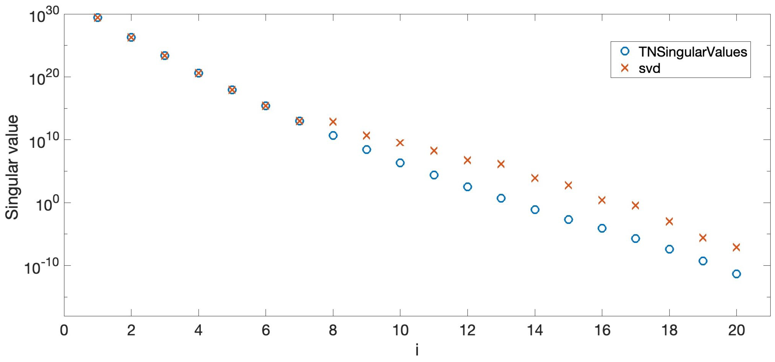
First, the singular values of the considered matrices, , were computed with Mathematica by using a 200 digit precision. Then, these singular values were obtained with Matlab in two different ways. The first one was acquired by using the Matlab function svd. The second one was obtained by using the function TNSingularValues of the software library TNTool (see [25]). Figure 1 shows the singular values for the case where . The differences between the singular values computed with and the ones obtained with svd for the case can be observed. Therefore, the obtained approximations are quite different, except for the greater singular values.
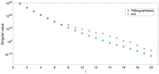
Figure 1.
Singular values for .
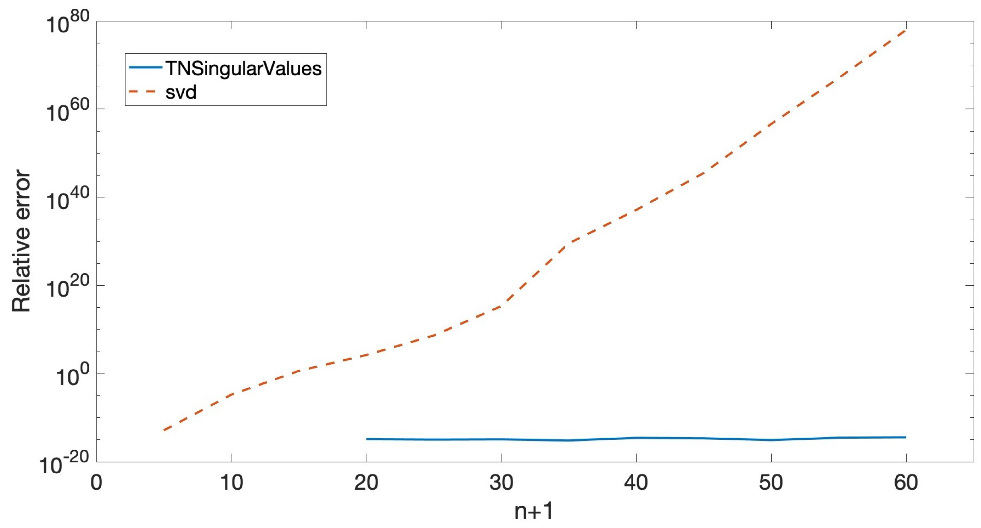
Then, the relative errors of the approximations of the obtained minimal singular values were computed considering the singular values provided by Mathematica as exact. It was observed that the lower the singular value is, the greater the relative error is for the usual standard method. Figure 2 shows these relative errors for the minimal singular values , , obtained in Matlab via these two different ways (svd and TNSingularValues). The figures are shown using a logarithmic scale for the Y-axis. Hence, when a relative error is zero for a certain , the line for that value does not appear (all the figures in this work showing relative errors use a logarithmic scale for the Y-axis). It can be observed that the results calculated with the new HRA algorithms (the algorithm obtaining the HRA bidiagonal decomposition of the matrix together with TNSingularValues) are very accurate in contrast to the poor results obtained with the standard algorithm.

Figure 2.
Relative errors when computing the singular values for .
Next, the systems of linear equations for were considered, where is the vector whose entries has an alternating pattern of signs. Moreover, its absolute values were randomly generated as integers in the interval . The systems were solved with Mathematica using 200 digits of precision, and the computed results were considered to be exact. Then, we solved the systems with Matlab in two different ways, like in the case of the singular values:
- 1.
- Using TNSolve and the bidiagonal decomposition of to HRA.
- 2.
- Using the Matlab operator \.
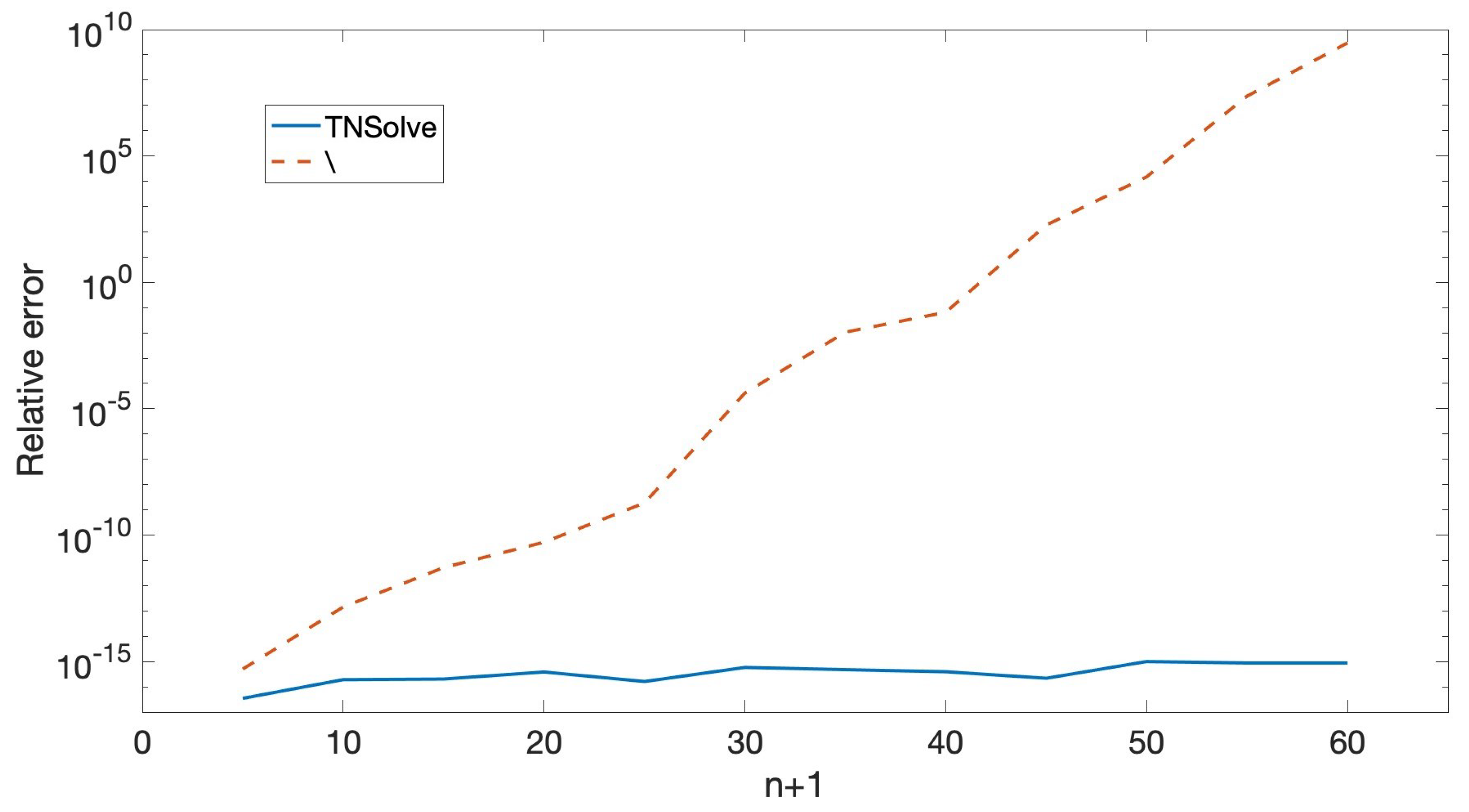
Then, the relative errors of the solutions obtained with Matlab were calculated, where are the solutions obtained with Mathematica. Figure 3 shows the results.
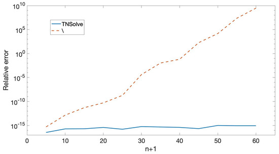
Figure 3.
, , when solving .
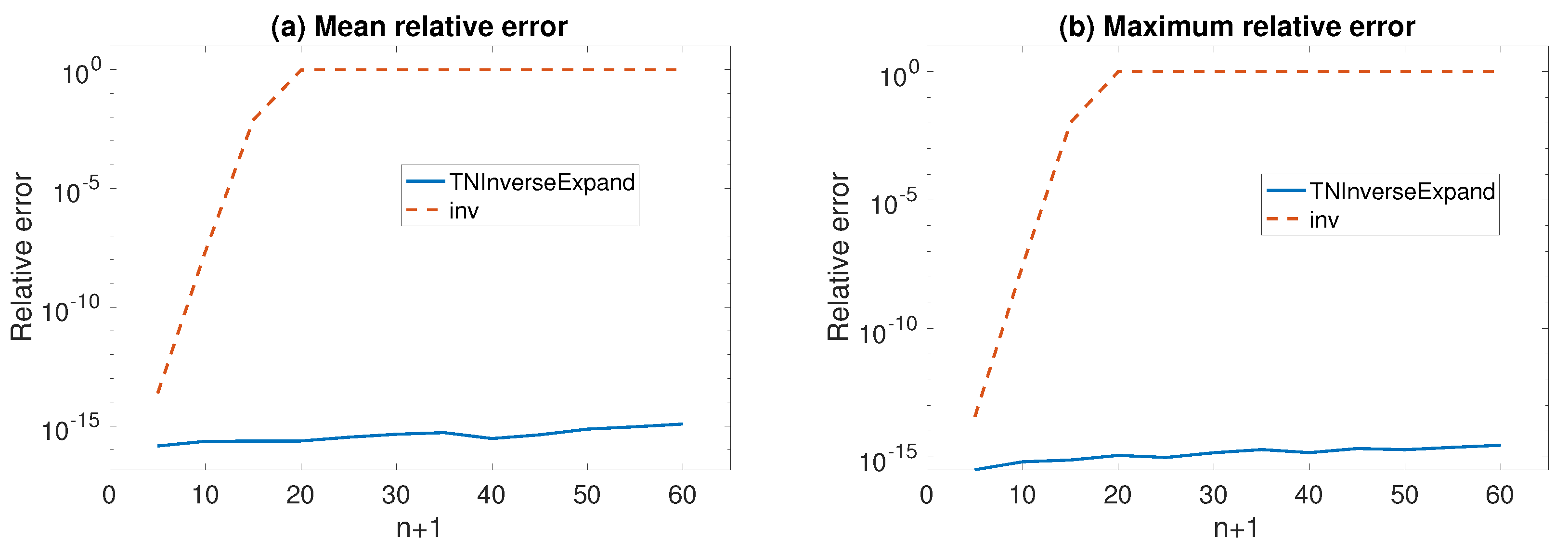
In the case of inverses , they were first obtained with Mathematica using a 200 digit precision. Then, they were calculated with Matlab in two ways. Firstly, using TNInverseExpand with the new HRA biadiagonal decomposition. Secondly, using the standard Matlab command inv. Then, component-wise relative errors corresponding to the approximations obtained using Matlab were computed, taking the results of Mathematica as being exact. Figure 4 shows the mean and the maximum of these component-wise relative errors.

Figure 4.
Mean and maximum component-wise relative errors when computing the inverse .
Taking into account the numerical results, we can see that the new methods introduced in this work outperform the standard algorithms for the three algebra problems that were considered.
4.2. Example 2
For this second example, the symmetric Pascal matrices defined by (14), for , in the case where x and y are given by (18), were considered. Since these matrices are not triangular, their eigenvalues were also computed with Matlab in two ways:
- 1.
- With the usual Matlab command eig.
- 2.
- With TNEigenValues of the library TNTool using the bidiagonal decomposition of the matrices to HRA given in Theorem 4.
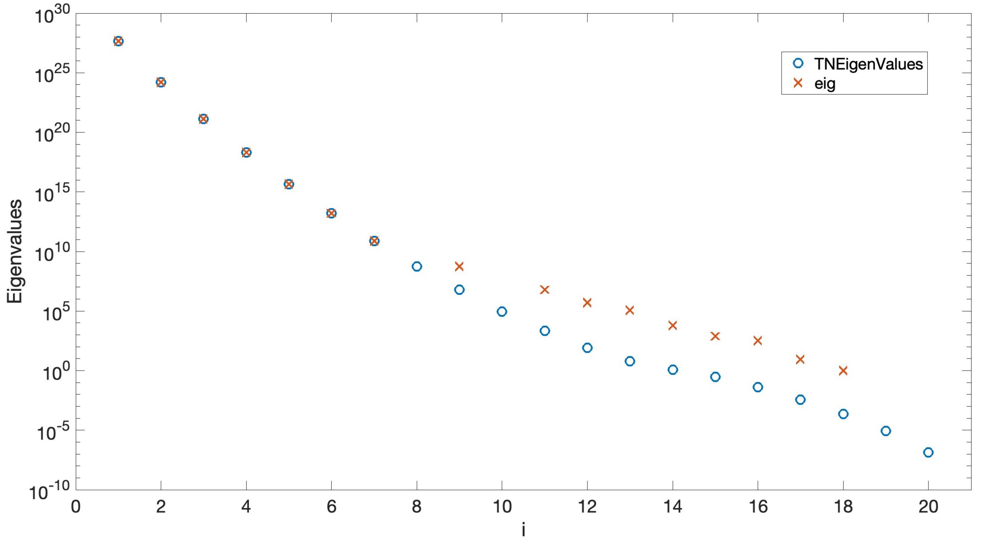
Figure 5 shows the eigenvalues computed in these two ways for the symmetric Pascal matrix . It can be observed than the approximation to the greater eigenvalues obtained with both methods are very similar, whereas the approximations to the lower eigenvalues are quite different. In fact, the eigenvalues of a nonsingular totally positive matrix are positive real numbers, and the eigenvalues of obtained with Matlab eig function are either negative real numbers or even complex numbers with a negative real part.
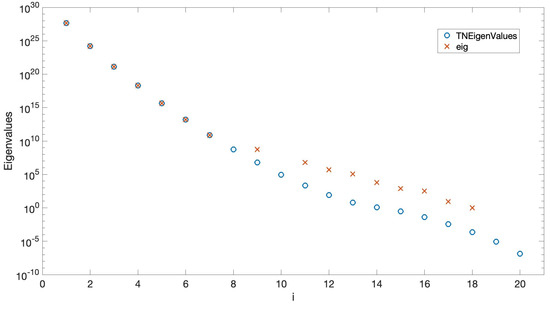
Figure 5.
Eigenvalues for .
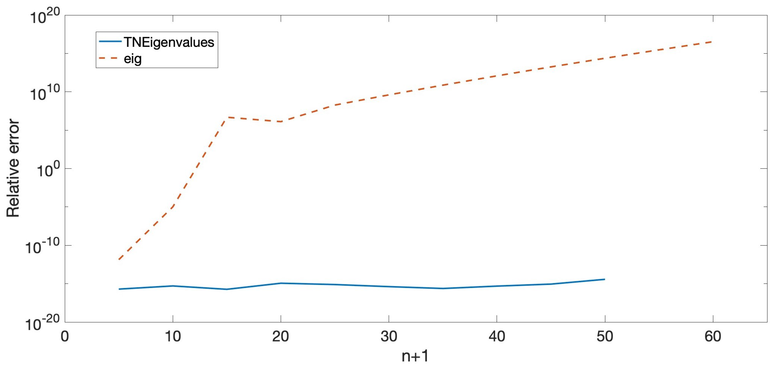
Then, the relative errors for the minimal eigenvalues of the considered matrices were calculated, taking the minimal eigenvalues provided by Mathematica with a 200-digit precision as exact. Figure 6 shows these relative errors. It can be observed that the approximations of the eigenvalues obtained with TNEigenValues and the new bidiagonal decomposition are much better than those obtained with the standard Matlab eig command.
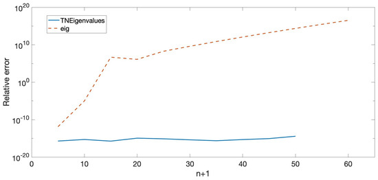
Figure 6.
Relative errors when computing the eigenvalues for .
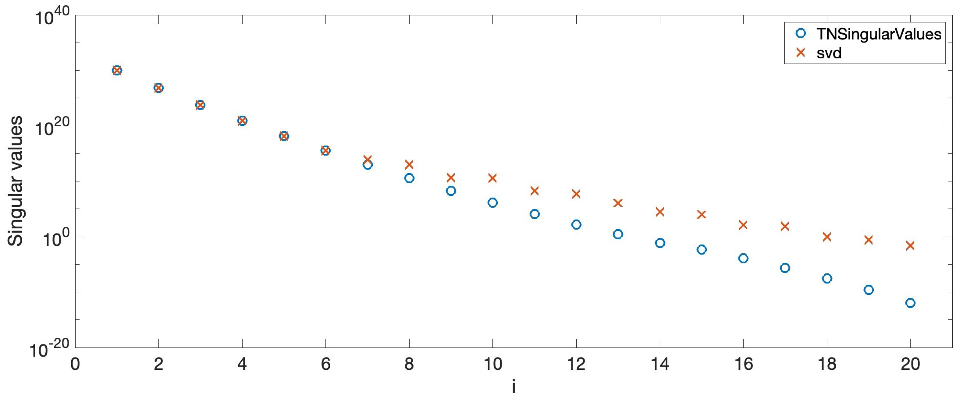
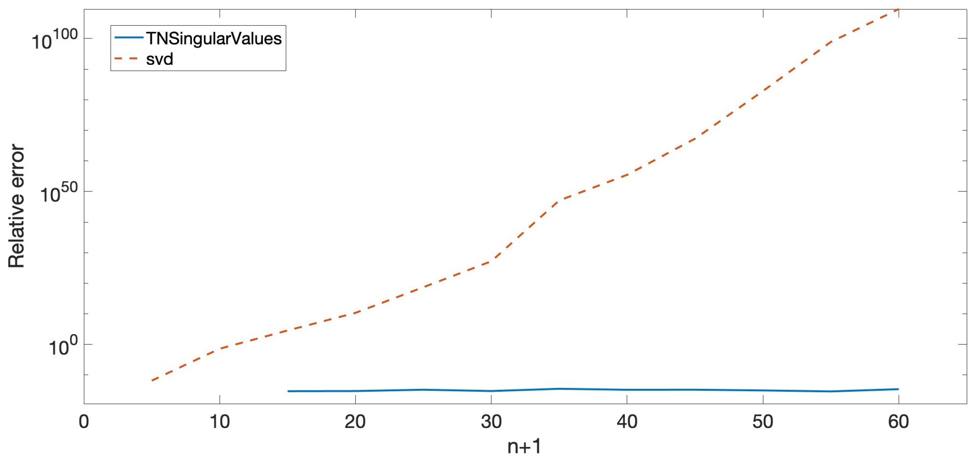
In addition, the same numerical tests of Example 1 were carried out for the symmetric Pascal matrices considered now. Figure 7 shows the approximations to the singular values of the matrix . The same conclusion for the case of eigenvalues is obtained, with the lower singular values being more prone to higher rounding errors. Thus, Figure 8 shows the relative errors for the minimal singular values of matrices.
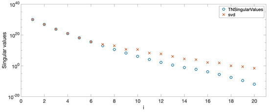
Figure 7.
Singular values for .
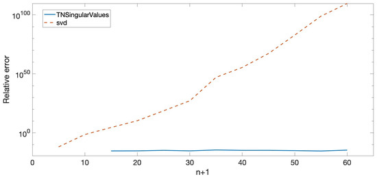
Figure 8.
Relative errors when computing the singular values for .
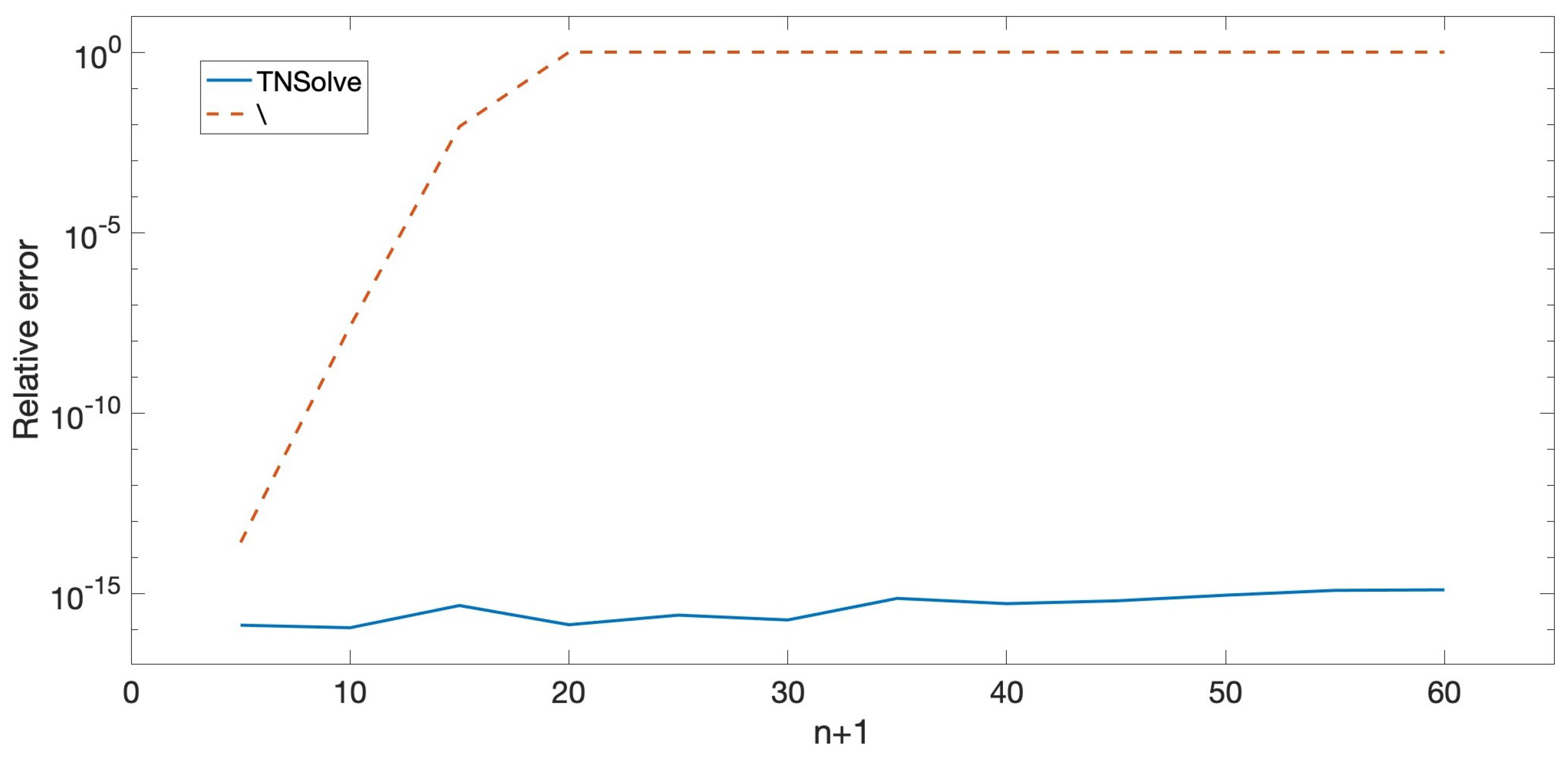
For the cases of linear systems of equations, 2-norm relative errors can be seen in Figure 9.
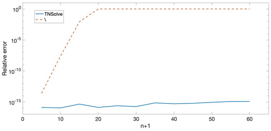
Figure 9.
, , when solving .
Finally, the mean and maximum component-wise relative errors for the computation of the inverses of symmetric Pascal matrices can be seen in Figure 10.
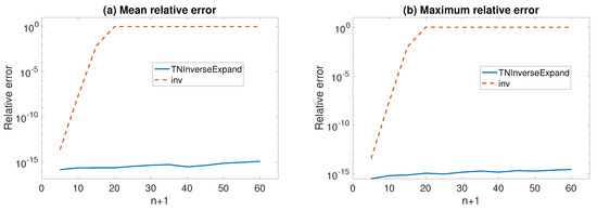
Figure 10.
Relative errors when computing the inverse .
5. Conclusions
Pascal k-eliminated functional matrices and Pascal symmetric functional matrices were studied previously in the literature. In this paper, we obtained the bidiagonal decomposition of these generalized Pascal matrices. Appropriate conditions, provided that these matrices were either totally positive or inverse of totally positive matrices, were found. In those cases, the bidiagonal decomposition can be performed with high relative accuracy. Consequently, many other linear algebra calculations with these matrices can be computed with high relative accuracy, for example, the calculation of their eigenvalues, singular values, inverses and of some associated linear systems. The high relative accuracy of the presented method was illustrated with some numerical examples.
Author Contributions
Conceptualization, J.D., H.O. and J.M.P.; Methodology, J.D., H.O. and J.M.P.; Software, J.D., H.O. and J.M.P.; Writing—original draft, J.D., H.O. and J.M.P.; Writing—review & editing, J.D., H.O. and J.M.P. All authors have read and agreed to the published version of the manuscript.
Funding
This research was partially supported through the Spanish research grants PID2022-138569NB-I00 and RED2022-134176-T (MCIU/AEI), and by Gobierno de Aragón (E41_23R).
Data Availability Statement
Data is contained within the article.
Conflicts of Interest
The authors declare no conflicts of interest.
Abbreviations
The following abbreviations are used in this manuscript:
| TP | Totally positive |
| HRA | High relative accuracy |
References
- Edelman, A.; Strang, G. Pascal Matrices. Am. Math. Mon. 2004, 111, 189–197. [Google Scholar] [CrossRef]
- Bayat, M. Generalized Pascal k-eliminated functional matrix with 2n variables. Electron. J. Linear Algebra 2011, 22, 419–429. [Google Scholar]
- Bayat, M.; Faal, H.T. Pascal k-eliminated functional matrix and its property. Linear Algebra Appl. 2000, 308, 65–75. [Google Scholar] [CrossRef]
- Lv, X.-G.; Huang, T.-Z.; Ren, Z.-G. A new algorithm for linear systems of the Pascal type. J. Comput. Appl. Math. 2009, 225, 309–315. [Google Scholar] [CrossRef]
- Zhang, Z. The linear algebra of the generalized Pascal matrix. Linear Algebra Appl. 1997, 250, 51–60. [Google Scholar] [CrossRef]
- Zhang, Z.; Liu, M. An extension of the generalized Pascal matrix and its algebraic properties. Linear Algebra Appl. 1998, 271, 169–177. [Google Scholar] [CrossRef]
- Alonso, P.; Delgado, J.; Gallego, R.; Peña, J.M. Conditioning and accurate computations with Pascal matrices. J. Comput. Appl. Math. 2013, 252, 21–26. [Google Scholar] [CrossRef]
- Delgado, J.; Orera, H.; Peña, J.M. Accurate bidiagonal decomposition and computation with generalized Pascal matrices. J. Comput. Appl. Math. 2021, 391, 113443. [Google Scholar] [CrossRef]
- Demmel, J.; Dumitriu, I.; Holtz, O.; Koev, P. Accurate and efficient expression evaluation and linear algebra. Acta Numer. 2008, 17, 87–145. [Google Scholar] [CrossRef]
- Demmel, J.; Gu, M.; Eisenstat, S.; Slapnicar, I.; Veselic, K.; Drmac, Z. Computing the singular value decomposition with high relative accuracy. Linear Algebra Appl. 1999, 299, 21–80. [Google Scholar] [CrossRef]
- Ando, T. Totally positive matrices. Linear Algebra Appl. 1987, 90, 165–219. [Google Scholar] [CrossRef]
- Gantmacher, F.P.; Krein, M.G. Oscillation Matrices and Kernels and Small Vibrations of Mechanical Systems, Revised ed.; AMS Chelsea Publishing: Providence, RI, USA, 2002. [Google Scholar]
- Gasca, M.; Peña, J.M. On factorizations of totally positive matrices. In Total Positivity and Its Applications; Gasca, M., Micchelli, C.A., Eds.; Kluver Academic Publishers: Dordrecht, The Netherlands, 1996; pp. 109–130. [Google Scholar]
- Gasca, M.; Micchelli, C.A. (Eds.) Total Positivity and Its Applications, Volume 359 of Mathematics and Its Applications; Kluwer Academic Publishers Group: Dordrecht, The Netherlands, 1996. [Google Scholar]
- Karlin, S. Total Positivity; Stanford University Press: Stanford, CA, USA, 1968; Volume I. [Google Scholar]
- Pinkus, A. Totally Positive Matrices. Tracts in Mathematics; Cambridge University Press: Cambridge, UK, 2010; Volume 181. [Google Scholar]
- Koev, P. Accurate eigenvalues and SVDs of totally nonnegative matrices. SIAM J. Matrix Anal. Appl. 2005, 27, 1–23. [Google Scholar] [CrossRef]
- Koev, P. Accurate computations with totally nonnegative matrices. SIAM J. Matrix Anal. Appl. 2007, 29, 731–751. [Google Scholar] [CrossRef]
- Demmel, J.; Koev, P. The accurate and efficient solution of a totally positive generalized Vandermonde linear system. SIAM J. Matrix Anal. Appl. 2005, 27, 142–152. [Google Scholar] [CrossRef]
- Marco, A.; Martínez, J.J. A fast and accurate algorithm for solving Bernstein-Vandermonde linear systems. Linear Algebra Appl. 2007, 422, 616–628. [Google Scholar] [CrossRef]
- Marco, A.; Martínez, J.J.; Viaña, R. Accurate bidiagonal decomposition of totally positive h-Bernstein-Vandermonde matrices and applications. Linear Algebra Appl. 2019, 579, 32. [Google Scholar] [CrossRef]
- Gasca, M.; Peña, J.M. Total positivity and Neville Elimination. Linear Algebra Appl. 1992, 165, 25–44. [Google Scholar] [CrossRef]
- Barreras, A.; Peña, J.M. Accurate computations of matrices with bidiagonal decomposition using methods for totally positive matrices. Numer. Linear Algebra Appl. 2013, 20, 413–424. [Google Scholar] [CrossRef]
- Marco, A.; Martínez, J.J. Accurate computation of the Moore-Penrose inverse of strictly totally positive matrices. J. Comput. Appl. Math. 2019, 350, 299–308. [Google Scholar] [CrossRef]
- Koev, P. Available online: https://sites.google.com/sjsu.edu/plamenkoev/home/software/tntool (accessed on 15 January 2025).
Disclaimer/Publisher’s Note: The statements, opinions and data contained in all publications are solely those of the individual author(s) and contributor(s) and not of MDPI and/or the editor(s). MDPI and/or the editor(s) disclaim responsibility for any injury to people or property resulting from any ideas, methods, instructions or products referred to in the content. |
© 2025 by the authors. Licensee MDPI, Basel, Switzerland. This article is an open access article distributed under the terms and conditions of the Creative Commons Attribution (CC BY) license (https://creativecommons.org/licenses/by/4.0/).

