Abstract
Fractional-order chaotic systems have received increasing attention over the past few years due to their ability to effectively model memory and complexity in nonlinear dynamics. Nonetheless, most of the research conducted so far has been on constant-order formulations, which still have some limitations in terms of adaptability and reality. Thus, to evade these limitations, we present a recently designed four-dimensional hyperchaotic Chen system with variable-order fractional (VOF) derivatives in the Liouville–Caputo sense. In comparison with constant-order systems, the new system possesses excellent performance in numerous aspects. Firstly, with the use of variable-order derivatives, the system becomes more adaptive and flexible, allowing the chaotic dynamics of the system to evolve with changing fractional orders. Secondly, large-scale numerical simulations are conducted, where phase portrait orbits and time series for differences in VOF directly illustrate the effect of the order function on the system’s behavior. Thirdly, qualitative analysis is performed with the help of phase portraits, time series, and Lyapunov exponents to confirm the system’s hyperchaotic behavior and sensitivity to initial and control parameters. Finally, the model developed demonstrates a wide range of dynamic behaviors, which confirms the sufficient efficiency of VOF calculus for modeling complicated nonlinear processes. Numerous analyses indicate that this research not only shows meaningful findings but also provides thoughtful methodologies that might result in subsequent research on fractional-order chaotic systems.
Keywords:
fractional calculus; variable-order derivatives; chaos; computational simulation; numerical solution MSC:
26A33; 34K37; 03D15; 65C30
1. Introduction
In recent years, fractional calculus, which extends classical integer-order integration and differentiation to a non-integer order, has drawn considerable interest because of its precise explanation of the strongly nonlinear dynamical behavior in contrast to the classical models [1]. Chaotic systems have attracted significant interest due to their wide-ranging applications in memristive hyperchaotic systems, Hopfield neural networks, and image encryption, motivating the study of their complex dynamics [2,3]. Fractional-order systems offer more flexible and realistic modeling platforms for engineering, biological, and physical systems [4,5], especially for the system where memory effects and long-range dependence are included [6].
Fractional-order systems are a generalization of conventional models in the sense that they incorporate memory effects and long-range dependencies, making them ideal to model real phenomena [7]. Compared to integer-order models, fractional systems are more flexible and accurate in modeling complex dynamics, particularly chaotic dynamics [8,9].
One of the primary advantages of fractional-order models is their ability to describe memory-dependent and long-range behavior. However, a constant-order derivative might be inadequate for systems with time-varying memory behavior [10]. In order to remedy this shortcoming, variable-order fractional derivatives were proposed, which allow time-dependent, spatial-dependent, or even other factor-dependent alteration of the differentiation order [11,12,13]. This new development allows for better modeling of nonuniform memory systems and, as a result, the application of fractional calculus to other areas of science and engineering. In particular, a comprehensive review of variable-order operators has been presented [14], novel neural variable-order fractional differential equation networks have been proposed for artificial intelligence tasks [15], and predictive modeling of CO2 emissions using gray models of nonlinear fractional order has been demonstrated [16].
To understand the stability, bifurcations, and chaotic properties of variable fractional systems, numerical solutions must be obtained using a variety of techniques [17,18,19]. There are growing real-world uses for fractional chaotic systems [20,21].
The general aim of this paper is to investigate a novel 4D hyperchaotic Chen system using variable-order fractional derivatives in order to guide qualitative research to tackle chaotic dynamics, bifurcation, and sensitivity analysis utilizing phase portraits. Furthermore, the qualitative dynamics of the time-dependent dynamical system are investigated on the basis of chaos theory. Phase portraits, time series, and Lyapunov exponents are employed to identify chaotic behavior in self-regulating dynamical systems. This paper presents some of the latest findings in nonlinear dynamical systems, and it also offers valuable tools for future research in this field.
The flow chart in Figure 1 represents a systematic method for studying the 4D Chen system. There are several analytical steps within the workflow that guarantee a systematic study of dynamical systems. On the left side of the workflow is a systematic investigation of variable-order fractional dynamical systems (VFDS) with dynamical stability checks and hypothesis formulation. The right side of the process consists of an entire characterization of a chaotic system that systematically covers chaos, bifurcation, Lyapunov exponents, phase trajectory, and time series. The two subjects are classified into two major sections for strategic reasons. Scholars can investigate the complex dynamics of the Chen system step by step owing to this well-designed format. This also allows for a multiperspective cognition that involves theoretical modeling, computational simulation, and empirical testing by the use of corresponding analytical tools.
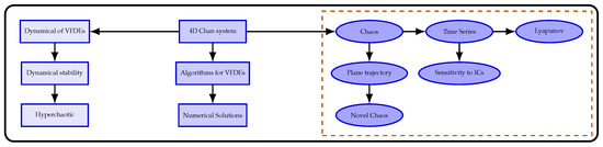
Figure 1.
Graphical abstract of perturbed dynamical system analysis.
In the analysis of the four-dimensional hyperchaotic fractional Chen system, the Table 1 demonstrates a broad range of research methods. These techniques indicate the huge number of tools applied in the analysis of the behavior of complex dynamical systems, whereas the majority of earlier studies were interested chiefly in classical quantities, such as Lyapunov exponents (LE), and chaotic (CH) or hyperchaotic (HCH) dynamics; in general, the current research is focused particularly on variable order fractional dynamical systems (VFDS) and the sensitivity of initial conditions (). Moreover, this research integrates the time series (TS) data analysis with emphasizing the role of numerical solutions (NS) in revealing the system dynamics. Not only does the new framework deepen the understanding of fractional-order chaos, but it also advances computational modeling and the ability to predict system evolution across different parameter regimes.

Table 1.
Comparison of studies on 4D hyperchaotic Chen system and chaos.
To fill the research vacuum in fluctuating-order fractional-order chaotic systems, the VOF system accommodates dynamics to evolve with fluctuating fractional orders whereby simulations confirm hyperchaotic dynamics, initial value sensitivity, and rich dynamics, thus confirming VOF calculus potential in subsequent fractional-order chaos research. In general, the principal contributions of this paper include the following:
- We address the intrinsic drawbacks of constant-order systems and offer a more practical framework for capturing memory and adaptability in nonlinear dynamics by presenting a recently developed four-dimensional (4D) hyperchaotic Chen system with variable-order fractional (VOF) derivatives in the Liouville–Caputo sense.
- The proposed system creatively exploits variable-order derivatives to enhance flexibility, enabling the chaotic dynamics to evolve with changing fractional orders. This design establishes a richer structure for analyzing dynamical transitions compared to fixed-order formulations.
- Phase-space orbits and time series for various are used in extensive numerical simulations to clearly show how the order function affects system behavior. These results demonstrate how important fractional order variability is in forming intricate dynamical responses.
- The system’s hyperchaotic nature and sensitivity to initial conditions and control parameters are confirmed by a thorough qualitative analysis that includes phase portraits, time series, and Lyapunov exponents. This method creates new avenues for methodically investigating the sensitivity and stability of VOF-based systems.
- The suggested model exhibits a wide variety of dynamic properties, proving the effectiveness and applicability of VOF calculus in simulating complex nonlinear processes. These contributions offer useful methodologies as well as theoretical insights that can direct future studies in fractional-order chaotic systems.
2. Preliminaries
This section gives definitions of the Liouville–Caputo fractional derivative in constant and variable orders, which form the mathematical basis of the proposed model. The Liouville–Caputo (LC) fractional derivative is an extension of the standard differentiation to orders beyond integers and hence provides a useful tool to describe memory and hereditary phenomena in physical and engineering processes. It is most useful in describing intricate processes with viscoelastic materials, anomalous diffusion, fractional-order control systems, and other processes where previous states play an important role in governing the system’s evolution as time progresses.
Definition 1
([29]). The Liouville–Caputo (LC) fractional derivative of constant order α is defined as
where
- : The Liouville–Caputo fractional derivative operator, where the order of the derivative changes with time .
- : The function being differentiated.
- ξ: The integration variable.
- : The Euler gamma function.
- : The variable fractional order of the derivative, which depends on time.
- : The kernel of the integral, where α.
- : The definite integral with respect to ξ.
Definition 2
([30]). The variable-order Liouville–Caputo (LCV) fractional derivative, where the order varies with time , is defined as
where
- : The Liouville–Caputo variable-order fractional derivative operator, where the order of the derivative changes with time .
- : The function being differentiated.
- ξ: The integration variable.
- : The Euler gamma function.
- : The variable fractional order of the derivative, which depends on time.
- : The kernel of the integral, where .
- : The definite integral with respect to ξ.
3. 4D Hyperchaotic Chen System
The hyperchaotic system examined in [31] is governed by the following set of differential equations:
where and denote the state variables, and are real-valued parameters.
Divergence of the 4D Hyperchaotic Chen System
To investigate the dissipative nature of the system, we compute the divergence of the corresponding vector field
, defined as
The divergence is calculated by taking the sum of the partial derivatives of each component with respect to its corresponding variable
Computing each term,
Thus, the total divergence becomes
If , then the system is dissipative.
4. Fractional 4D Hyperchaotic Chen System
The fractional hyperchaotic system examined in [32] is governed by the following set of differential equations:
where and denote state variables, and are parameters with real values [32].
4.1. Stability Analysis in Fractional Framework
Equilibrium Points
The fractional system in Equation (7) has equilibria at constant states; hence, we set the Caputo-like derivatives to zero and solve the algebraic system
- Step 1. Immediate relations
From the first and fourth equations of Equation (8) (noting ) we obtain
- Step 2. Solve for
- Step 3. Solve for
Use in the second equation and rearrange,
- Step 4. Equilibrium point (parameters)
Substituting , we obtain
Using numerical values with we get
The corresponding Jacobian matrix of Equation (7) is given by
The corresponding eigenvalues of the Jacobian at this equilibrium point are
This result indicates that the equilibrium point behaves as a saddle point and, consequently, is unstable.
Analyze the local stability of the fractional-order system. We define the matrix
where J denotes the Jacobian matrix evaluated at the equilibrium point, represents the corresponding fractional orders associated with each state variable, and M is the smallest positive integer such that for all i.
The equilibrium point is said to be asymptotically stable if all eigenvalues of the characteristic equation
satisfy the condition
This leads to a practical inequality used to assess stability,
If inequality holds true, the equilibrium point is considered asymptotically stable. On the other hand, for the system to exhibit chaotic dynamics (such as a strange attractor), the opposite condition must be satisfied,
We compute the minimum argument of the eigenvalues. If the fractional order satisfies the inequality, then
Since two eigenvalues (, ) have strictly positive real parts, they violate the angle condition required by Matignon’s criterion. Therefore, the equilibrium point is unstable for all . As a result, depending on the system parameters and initial conditions, the system may exhibit chaotic, hyperchaotic, or other complex unstable dynamics.
4.2. Stability Analysis in Fractional Variable-Order System
Consider the following fractional variable-order system:
with initial condition , where
- is the order function;
- is the input function;
- is the state function;
- and are constant matrices.
Assume that the matrix is invertible, where I denotes the identity matrix. This assumption guarantees the existence of solutions of Equation (10). Under this condition, Equation (10) can be equivalently expressed as
or, equivalently,
with the initial condition .
We now present a stability condition for Equation (10).
Proposition 1.
Proof.
Introduce the notation
for . Observe that
Since , we have
Moreover,
The linear part is governed by the constant matrix A, while collects the nonlinear terms. According to the same reasoning as in Proposition 1, the variable-order system in Equation (16) is asymptotically stable if all eigenvalues of A satisfy
for every .
Equation (17) ensures that the contribution of the variable-order memory kernel does not dominate the dynamics of the linearized Chen system. Hence, the stability of the 4D hyperchaotic Chen system under variable-order derivatives can be guaranteed using the same framework established for the general fractional variable-order system.
The stability of variable-order fractional systems has been widely studied in theory as well as applications. General conclusions on the solvability, difference systems, and asymptotic stability can be found in [33,34]. Also, studies on high-dimensional chaotic and hyperchaotic networks, Lorenz-type and Chen-type networks.
In particular, with the imposition of spectral conditions on the linear part of the system matrix and suitable bounds on the variable-order kernel, asymptotic stability of the system can be guaranteed.
4.3. Variable Order Fractional 4D Hyperchaotic Chen System
In this section, we present the 4D hyperchaotic variational order system. While the integer-order and constant-order fractional forms of the 4D hyperchaotic Chen system were already studied [31,32], the present work’s contribution lies in how the system is placed in the variable-order fractional calculus framework. To this extent, the paper’s innovation does not lie in showing a new system but in how it brings variable-order derivatives to bear on the established 4D Chen system and studies its resulting dynamical behavior.
The hyperchaotic system is driven by the fractional derivative , where and denote state variables.
5. Numerical Algorithms for Variable-Order Fractional Systems
In this part we approximate solutions of models with Liouville–Caputo operators using numerical methods from [35]. The system is given by
Here, * denotes a chosen variable-order fractional derivative, is the initial condition (see Definition 2), and approximates at , with uniform steps over .
Evaluating at , the equation becomes
Applying a second-order Lagrange interpolation, the function over the interval is approximated as
Equations (24) and (25) are derived with the aid of a second-order Lagrange interpolation to estimate the nonlinear function on the subinterval . The interpolation produces a piecewise polynomial estimate of , and upon substitution into the discretized integral formulation of the fractional operator, it leads directly to the formulations. For ease of calculation, we define the following expressions:
Hence, the numerical approximations of the variable-order LC-type system are expressed as
where .
where .
where .
where .
The numerical values in Table 2, Table 3 and Table 4 show that the system exhibits very different behaviors under the variable-order functions , , and . Although all simulations are initialized with the same initial conditions, the trajectories show remarkably different paths as time progresses, reflecting the system’s sensitivity to the precise shape of the variable-order function. The cosine-modulated case (Table 2) exhibits amplitude oscillation that is seemingly quasi-periodic in character, with oscillation cycles in positive and negative directions on all variables. Contrarily, the tanh-driven case (Table 3) induces steeper transition dynamics and higher peak amplitudes, which indicates greater nonlinear effects. The sine-controlled case (Table 4) produces more gradual oscillatory behavior with moderate oscillations in amplitude, yet still noticeably exhibits chaotic phenomena. These analogies are used to outline how the form of the fractional-order function influences the temporal development of the system directly and illustrate the greater flexibility and sophistication introduced by variable-order fractional dynamics.
Table 2.
System results using numerical algorithm with .
Table 3.
System results using numerical algorithm with .
Table 4.
System results using numerical algorithm with .
6. Dynamical Analysis
This section analyzes the chaotic nature of the system using analytical tools such as time series plots, Lyapunov exponents, and attractors (18). Chaos is revealed by high sensitivity to initial conditions, where small changes produce divergent trajectories. The Lyapunov exponent measures this sensitivity, while time series and phase projections demonstrate the system’s unpredictable, non-repeating behavior within its state space. The figures were drawn with the help of the package of MATLAB software (R2024a).
6.1. Dynamics in Phase Portrait
We investigate the chaotic dynamics of the system defined in Equation (18), numerical simulations for three different scenarios. The corresponding phase portraits, presented in Figure 2, Figure 3, Figure 4, Figure 5, Figure 6 and Figure 7, illustrate the system’s behavior under each condition.
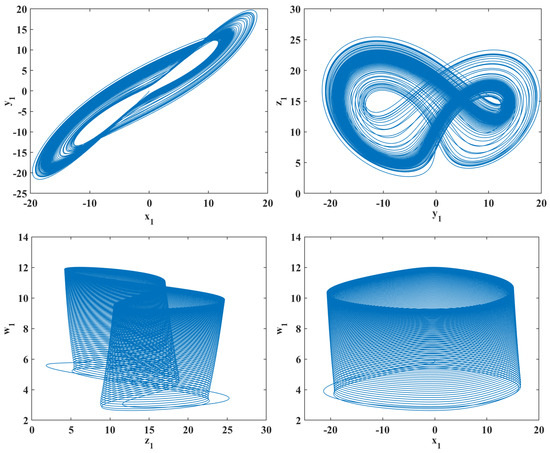
Figure 2.
Phase portraits of a dynamical system with Case 1.
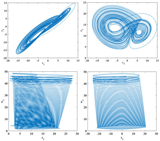
Figure 3.
Phase portraits of a dynamical system with Case 2.
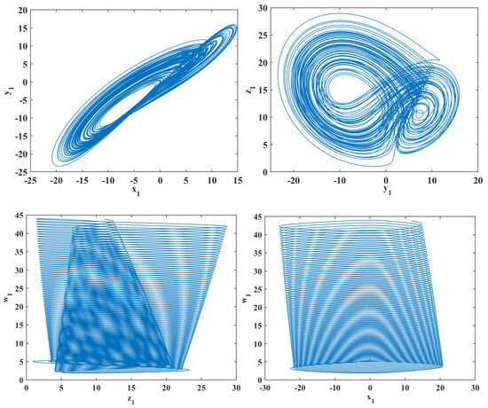
Figure 4.
Phase portraits of a dynamical system with Case 3.
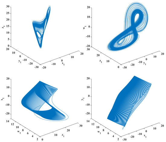
Figure 5.
Phase portraits of the 4D hyperchaotic Chen system with variable-order function , showing complex trajectories and sensitive dependence on initial conditions.
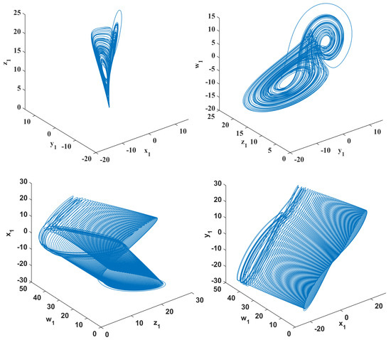
Figure 6.
Phase portraits of the 4D hyperchaotic Chen system with variable-order function , illustrating periodic modulation effects on the hyperchaotic dynamics.
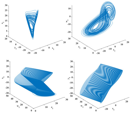
Figure 7.
Phase portraits of the 4D hyperchaotic Chen system with variable-order function , highlighting the system’s transition in behavior due to the sigmoidal change in the order.
The system involves four state variables: and , and five real-valued parameters defined as
The initial conditions for all cases are given by
The system is analyzed under three different scenarios of the variable-order function as follows:
- Case 1: .
- Case 2: .
- Case 3: .
The system was considered numerically for three specific cases of the variable-order function to investigate its chaotic behavior. These were chosen such that they encompass various kinds of functional variation—hyperbolic, periodic, and sigmoidal—hence allowing us to observe the system response towards varying fractional orders; while these are representative cases, they do qualitatively demonstrate the effect of on the system behavior.
Figure 3 illustrates the emergence of chaotic behavior, showing the complex rules exhibited by the system in this case. In scenarios, the presence of chaotic attractors is evident through the distinct phase portraits. Variations in the functional form of contribute to noticeable differences in the trajectories of the system.
6.2. Time Series Analysis
Time series in Figure 8, Figure 9 and Figure 10 reveal that the system displays complex dynamics with signs of chaos, especially through non-periodic oscillations and initial condition sensitivity. This is compounded by Lyapunov exponent analysis presented in the following section, where the divergence of neighboring orbits in the phase portrait is quantified.
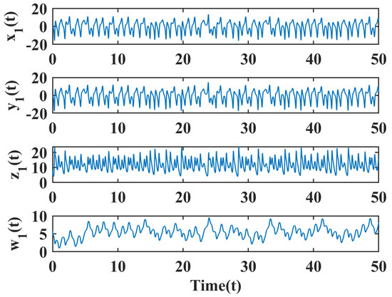
Figure 8.
Time series of the system for Case 1.
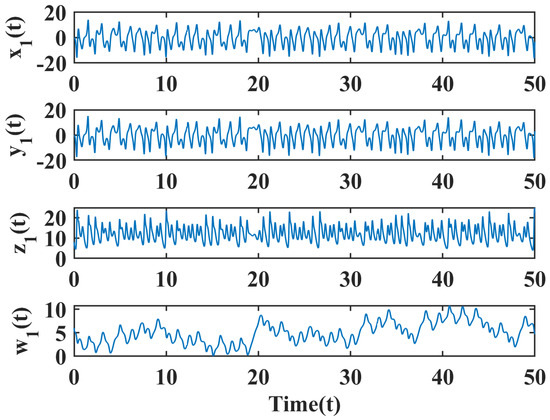
Figure 9.
Time series of the system for Case 2.
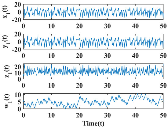
Figure 10.
Time series of the system for Case 3.
6.3. Lyapunov Exponents
The Lyapunov exponent in Figure 11, Figure 12 and Figure 13 measures the rate at which adjacent trajectories in the state space of a system diverge or converge and is central to determining the sensitivity of a system to initial conditions and the emergence of complex behavior, especially for fractional-order systems. The most significant in determining the general dynamics of a system is the largest Lyapunov exponent (LLE). A positive LLE is associated with chaotic behavior by exponential divergence, a negative one with stability by convergence, and a zero one with neutral stability. Calculation of the LLE for the system (18) under variable order conditions provides a clear picture of its dynamic complexity and allows the transitions between chaotic and stable regimes to be determined. The following algorithm was used to compute the Lyapunov exponents [36].
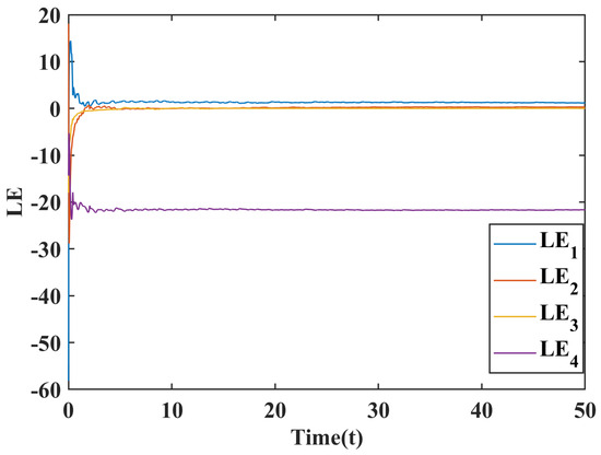
Figure 11.
Lyapunov exponents over time for Case 1.
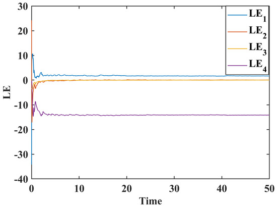
Figure 12.
Lyapunov exponents over time for Case 2.
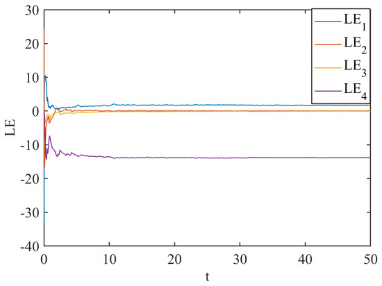
Figure 13.
Lyapunov exponents over time for Case 3.
Table 5 numerically confirms the hyperchaotic character of the system, as at least two positive Lyapunov exponents are found in all the cases. The results indicate high initial condition sensitivity and complex dynamics, with the largest exponent increasing as the variable-order function changes, exhibiting the impact of fractional order on chaotic behavior of the system.
Table 5.
Lyapunov exponents versus of a fractional system.
6.4. Sensitivity Analysis
The system’s sensitivity to initial conditions is demonstrated in Figure 14, Figure 15, Figure 16, Figure 17, Figure 18 and Figure 19, where even small differences in the initial values lead to dramatically different oscillatory dynamics. The system with (0, 0.3, 6, 8) (Figure 14), for example, has lighter, gentler oscillations at the beginning, whereas the system with (1, 0.5, 3, 4) (Figure 15) already exhibits more pronounced and erratic dynamics from the start. This sensitivity with these constant parameters (, , , , ) indicates the nonlinearity and perhaps chaotic nature of the system and the need to choose the initial conditions with care in practical situations so as not to obtain unpredictable results. The time series plots for each state variable in Case 1 are shown in (Figure 14 and Figure 15), demonstrating aperiodic long-term behavior that demonstrates the existence of chaos in the system. The time series plots for Case 2 are similarly shown in (Figure 16 and Figure 17), also in Case 3 in (Figure 18 and Figure 19), where each state variable exhibits chaotic variations.
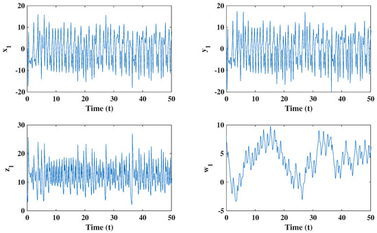
Figure 14.
Time series for Case 1 with initial conditions .
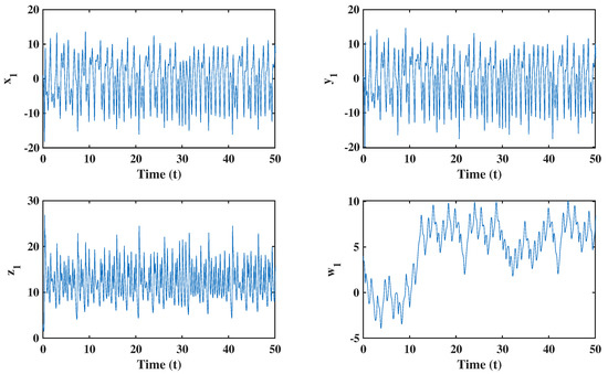
Figure 15.
Time series for Case 1 with initial conditions .
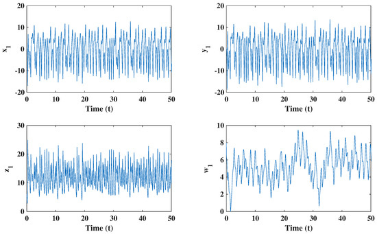
Figure 16.
Time series for Case 2 with initial conditions .
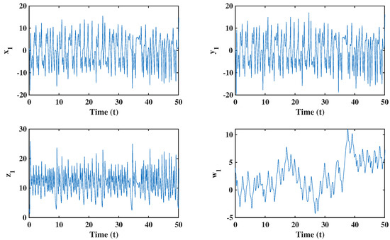
Figure 17.
Time series for Case 2 with initial conditions .
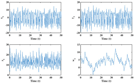
Figure 18.
Time series for Case 3 with initial conditions .
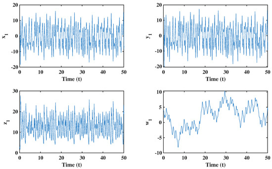
Figure 19.
Time series for Case 3 with initial conditions .
The results show that the Chen system of hyperchaotic 4D variables of order possesses complex dynamics dominated by the fractional order function . Phase portraits show complex orbits, while time series detect non-periodic oscillations and high initial condition sensitivity. Lyapunov exponents confirm hyperchaotic behavior and sensitivity analyses emphasize the importance of initial states.
7. Conclusions
In this study, to explore the complex dynamics of higher-dimensional systems, we first constructed a 4D hyperchaotic Chen system via variable-order fractional calculus using the Liouville–Caputo derivative. Using numerical simulations performed in MATLAB, including phase portraits, time series, and Lyapunov exponents, we explained how variable-order derivatives influence system behavior. The results indicate that the system exhibits rich hyperchaotic dynamics, large initial sensitivity, and extensive memory effects, which justifies the function of the order function in its development.
Moreover, using derivative applications of variable order, we gained a deeper understanding of the time dynamics and adaptability of fractional order systems. The findings suggest that system parameters and the order function play a crucial role in controlling hyperchaotic behavior and determining phase-space trajectories. Such findings provide a solid foundation for studying complex nonlinear dynamics in higher-order systems.
Despite its advantages, the proposed VOF hyperchaotic Chen system has some limitations, including reliance on numerical simulations and higher computational cost. In the future, we intend to extend this approach to solve new fractional models and compare it with other analytical and numerical approaches [37]. This research will further advance the science and engineering practice of variable-order fractional systems.
Author Contributions
Methodology, A.I.A., M.E., A.M.A., M.A.M.A., M.E.D., and I.K.; investigation, A.I.A., M.E., A.M.A., M.A.M.A., M.E.D., and I.K.; review and editing, A.I.A., M.E., A.M.A., M.A.M.A., M.E.D., and I.K.; writing—original draft, A.I.A., M.E., A.M.A., M.A.M.A., M.E.D., and I.K.; formal analysis, A.I.A., M.E., A.M.A., M.A.M.A., M.E.D., and I.K.; softwear, A.I.A., M.E., A.M.A., M.A.M.A., M.E.D., and I.K. All authors have read and agreed to the published version of the manuscript.
Funding
This research received no external funding.
Data Availability Statement
The original contributions presented in this study are included in the article. Further inquiries can be directed to the corresponding authors.
Conflicts of Interest
The authors declare no conflicts of interest.
References
- Hafez, M.; Alshowaikh, F.; Voon, B.W.N.; Alkhazaleh, S.; Al-Faiz, H. Review on recent advances in fractional differentiation and its applications. Progr. Fract. Differ. Appl. 2025, 11, 245–261. [Google Scholar]
- Feng, W.; Zhang, K.; Zhang, J.; Zhao, X.; Chen, Y.; Cai, B.; Zhu, Z.; Wen, H.; Ye, C. Integrating Fractional-Order Hopfield Neural Network with Differentiated Encryption: Achieving High-Performance Privacy Protection for Medical Images. Fractal Fract. 2025, 9, 426. [Google Scholar] [CrossRef]
- Li, H.; Yu, S.; Feng, W.; Chen, Y.; Zhang, J.; Qin, Z.; Zhu, Z.; Wozniak, M. Exploiting dynamic vector-level operations and a 2D-enhanced logistic modular map for efficient chaotic image encryption. Entropy 2023, 25, 1147. [Google Scholar] [CrossRef]
- Elbadri, M.; AlMutairi, D.M.; Almutairi, D.; Hassan, A.A.; Hdidi, W.; Abdoon, M.A. Efficient numerical techniques for investigating chaotic behavior in the fractional-order inverted Rössler system. Symmetry 2025, 17, 451. [Google Scholar] [CrossRef]
- Abdoon, M.A. Fractional Derivative Approach for Modeling Chaotic Dynamics: Applications in Communication and Engineering Systems. In International Conference on Mathematical Modelling, Applied Analysis and Computation; Springer: Cham, Switzerland, 2025; pp. 82–95. [Google Scholar]
- E. Alsubaie, N.; EL Guma, F.; Boulehmi, K.; Al-kuleab, N.; A. Abdoon, M. Improving influenza epidemiological models under Caputo fractional-order calculus. Symmetry 2024, 16, 929. [Google Scholar] [CrossRef]
- Wu, L.; Chen, Y. Fractional Grey System Model and Its Application; Springer: Singapore, 2025. [Google Scholar]
- Zhang, Y.; Sun, H.; Stowell, H.H.; Zayernouri, M.; Hansen, S.E. A review of applications of fractional calculus in Earth system dynamics. Chaos Solitons Fractals 2017, 102, 29–46. [Google Scholar] [CrossRef]
- Elgezouli, D.E.; Eltayeb, H.; Abdoon, M.A. Novel GPID: Grünwald–Letnikov Fractional PID for Enhanced Adaptive Cruise Control. Fractal Fract. 2024, 8, 751. [Google Scholar] [CrossRef]
- Samko, S.G. Fractional integration and differentiation of variable order. Anal. Math. 1995, 21, 213–236. [Google Scholar] [CrossRef]
- Almutairi, D.; AlMutairi, D.M.; Taha, N.E.; Dafaalla, M.E.; Abdoon, M.A. Variable-Fractional-Order Nosé–Hoover System: Chaotic Dynamics and Numerical Simulations. Fractal Fract. 2025, 9, 277. [Google Scholar] [CrossRef]
- Malaikah, H.; Al-Abdali, J.F. Variable-Order Fractional Derivatives in Financial Systems. Appl. Math. 2025, 16, 461–469. [Google Scholar] [CrossRef]
- Naik, P.A.; Naveen, S.; Parthiban, V.; Qureshi, S.; Alquran, M.; Senol, M. Advancing lotka-volterra system simulation with variable fractional order caputo derivative for enhanced dynamic analysis. J. Appl. Anal. Comput. 2025, 15, 1002–1019. [Google Scholar] [CrossRef]
- Patnaik, S.; Hollkamp, J.P.; Semperlotti, F. Applications of variable-order fractional operators: A review. Proc. R. Soc. A 2020, 476, 20190498. [Google Scholar] [CrossRef]
- Cui, W.; Kang, Q.; Li, X.; Zhao, K.; Tay, W.P.; Deng, W.; Li, Y. Neural variable-order fractional differential equation networks. In Proceedings of the AAAI Conference on Artificial Intelligence, Philadelphia, PA, USA, 25 February–4 March 2025; Volume 39, pp. 16109–16117. [Google Scholar]
- Jiang, H.; Jiang, P.; Kong, P.; Hu, Y.C.; Lee, C.W. A predictive analysis of China’s CO2 emissions and OFDI with a nonlinear fractional-order grey multivariable model. Sustainability 2020, 12, 4325. [Google Scholar] [CrossRef]
- Hassani, H.; Machado, J.T.; Avazzadeh, Z. An effective numerical method for solving nonlinear variable-order fractional functional boundary value problems through optimization technique. Nonlinear Dyn. 2019, 97, 2041–2054. [Google Scholar] [CrossRef]
- Parovik, R.; Tverdyi, D. Some Aspects of Numerical Analysis for a Model Nonlinear Fractional Variable Order Equation. Math. Comput. Appl. 2021, 26, 55. [Google Scholar] [CrossRef]
- Bhrawy, A.; Zaky, M. Numerical algorithm for the variable-order Caputo fractional functional differential equation. Nonlinear Dyn. 2016, 85, 1815–1823. [Google Scholar] [CrossRef]
- Sun, H.; Chang, A.; Zhang, Y.; Chen, W. A review on variable-order fractional differential equations: Mathematical foundations, physical models, numerical methods and applications. Fract. Calc. Appl. Anal. 2019, 22, 27–59. [Google Scholar] [CrossRef]
- Zhang, H.; Liu, F.; Phanikumar, M.S.; Meerschaert, M.M. A novel numerical method for the time variable fractional order mobile–immobile advection–dispersion model. Comput. Math. Appl. 2013, 66, 693–701. [Google Scholar] [CrossRef]
- Yang-Zheng, L.; Chang-Sheng, J.; Chang-Sheng, L.; Yao-Mei, J. Chaos synchronization between twodifferent 4D hyperchaotic Chen systems. Chin. Phys. 2007, 16, 660. [Google Scholar] [CrossRef]
- Alexan, W.; El-Damak, D.; Gabr, M. Image encryption based on fourier-DNA coding for hyperchaotic chen system, chen-based binary quantization S-box, and variable-base modulo operation. IEEE Access 2024, 12, 21092–21113. [Google Scholar]
- Cafagna, D.; Grassi, G. Bifurcation and chaos in the fractional-order Chen system via a time-domain approach. Int. J. Bifurc. Chaos 2008, 18, 1845–1863. [Google Scholar] [CrossRef]
- Čermák, J.; Nechvátal, L. Stability and chaos in the fractional Chen system. Chaos Solitons Fractals 2019, 125, 24–33. [Google Scholar] [CrossRef]
- Lu, J.G.; Chen, G. A note on the fractional-order Chen system. Chaos Solitons Fractals 2006, 27, 685–688. [Google Scholar] [CrossRef]
- Elbadri, M.; Abdoon, M.A.; Almutairi, D.; Almutairi, D.M.; Berir, M. Numerical Simulation and Solutions for the Fractional Chen System via Newly Proposed Methods. Fractal Fract. 2024, 8, 709. [Google Scholar] [CrossRef]
- Hussain, S.; Bashir, Z.; Malik, M.A. Chaos analysis of nonlinear variable order fractional hyperchaotic Chen system utilizing radial basis function neural network. Cogn. Neurodyn. 2024, 18, 2831–2855. [Google Scholar] [CrossRef] [PubMed]
- Oldham, K.; Spanier, J. The Fractional Calculus Theory and Applications of Differentiation and Integration to Arbitrary Order; Elsevier: Amsterdam, The Netherlands, 1974; Volume 111. [Google Scholar]
- Solís-Pérez, J.; Gómez-Aguilar, J.; Atangana, A. Novel numerical method for solving variable-order fractional differential equations with power, exponential and Mittag-Leffler laws. Chaos Solitons Fractals 2018, 114, 175–185. [Google Scholar] [CrossRef]
- Gao, T.; Chen, Z.; Yuan, Z.; Chen, G. A hyperchaos generated from Chen’s system. Int. J. Mod. Phys. C 2006, 17, 471–478. [Google Scholar] [CrossRef]
- Wu, X.; Lu, H.; Shen, S. Synchronization of a new fractional-order hyperchaotic system. Phys. Lett. A 2009, 373, 2329–2337. [Google Scholar] [CrossRef]
- Mozyrska, D.; Oziablo, P.; Wyrwas, M. Stability of fractional variable order difference systems. Fract. Calc. Appl. Anal. 2019, 22, 807–824. [Google Scholar] [CrossRef]
- Ostalczyk, P. Stability analysis of a discrete-time system with a variable-, fractional-order controller. Bull. Pol. Acad. Sci. Tech. Sci. 2010, 613–619. [Google Scholar] [CrossRef]
- Alqahtani, A.M.; Chaudhary, A.; Dubey, R.S.; Sharma, S. Comparative analysis of the chaotic behavior of a five-dimensional fractional hyperchaotic system with constant and variable order. Fractal Fract. 2024, 8, 421. [Google Scholar] [CrossRef]
- Wolf, A.; Swift, J.B.; Swinney, H.L.; Vastano, J.A. Determining Lyapunov exponents from a time series. Phys. D Nonlinear Phenom. 1985, 16, 285–317. [Google Scholar] [CrossRef]
- Abdoon, M.A.; Elbadri, M.; Alzahrani, A.B.; Berir, M.; Ahmed, A. Analyzing the inverted fractional rössler system through two approaches: Numerical scheme and lham. Phys. Scr. 2024, 99, 115220. [Google Scholar] [CrossRef]


Disclaimer/Publisher’s Note: The statements, opinions and data contained in all publications are solely those of the individual author(s) and contributor(s) and not of MDPI and/or the editor(s). MDPI and/or the editor(s) disclaim responsibility for any injury to people or property resulting from any ideas, methods, instructions or products referred to in the content. |
© 2025 by the authors. Licensee MDPI, Basel, Switzerland. This article is an open access article distributed under the terms and conditions of the Creative Commons Attribution (CC BY) license (https://creativecommons.org/licenses/by/4.0/).