Abstract
Increasing the amount of data with complex dynamics requires the constant updating of statistical distributions. This study aimed to introduce a new three-parameter distribution, named the new exponentiated Weibull (NEW) distribution, by applying the logarithmic transformation to the exponentiated Weibull distribution. The exponentiated Weibull distribution is a powerful generalization of the Weibull distribution that includes several classical distributions as special cases—Weibull, exponential, Rayleigh, and exponentiated exponential—which make it capable of capturing diverse forms of hazard functions. By combining the advantages of the logarithmic transformation and exponentiated Weibull, the new distribution offers great flexibility in modeling different forms of hazard functions, including increasing, J-shaped, reverse-J-shaped, and bathtub-shaped functions. Some mathematical properties of the NEW distribution were studied. Moreover, four different methods of estimation—the maximum likelihood (ML), least squares (LS), Cramer–Von Mises (CVM), and percentile (PE) methods—were employed to estimate the distribution parameters. To assess the performance of the estimates, three simulation studies were conducted, showing the benefit of the ML method, followed by the PE method, in estimating the model parameters. Additionally, five datasets were used to evaluate the effectiveness of the new distribution in fitting real data. Compared with some Weibull-type extensions, the results demonstrate the superiority of the new distribution in modeling various forms of real data and provide evidence for the applicability of the new distribution.
MSC:
62E10; 62E15; 60E05
1. Introduction
In real phenomena, data may not always be well captured by classical distributions. Thus, statistical distributions are continuously updated and improved in an attempt to accommodate the growth and complexity of data and enhance their fit. Researchers have considered proposing new methods to introduce new distributions with a good ability to fit various types of data in different applications. Some methods have focused on adding a new parameter to traditional distributions, such as the Marshall and Olkin [1], exponentiated [2], and alpha-power [3] methods, while others use any statistical distribution as a generator for new ones, such as the transformed-transformer (T-X) method [4]. These approaches have been utilized widely to generate highly adaptable generalizations of many well-known distributions. Examples include the exponentiated Chen distribution [5], the alpha-power Kumaraswamy distribution [6], the Marshall–Olkin odd Burr III exponential distribution [7], the exponentiated Gompertz distribution [8], the Marshall–Olkin Bilal distribution [9], the extended Weibull distribution [10], the exponentiated XLindley distribution [11], the alpha-power modified Weibull geometric distribution [12], and the alpha-power Erlang distribution [13], among others.
The Weibull distribution is the most commonly applied distribution in lifetime analyses and reliability engineering. Although it has great flexibility in modeling the monotone failure rates for many phenomena, it performs poorly when modeling non-monotonic hazard rate functions, which are common in medical applications and reliability. This limitation has motivated researchers to introduce different extensions of the Weibull distribution to enhance its ability to capture non-monotone hazards. For example, Ref. [14] presents the modified Weibull distribution, Ref. [15] proposes the Kumaraswamy Weibull distribution, Ref. [16] provides the generalized inverse Weibull distribution, Ref. [17] introduces the exponential Weibull distribution, Ref. [18] presents the odd Weibull Weibull distribution, Ref. [19] formulated the odd generalized exponential Weibull distribution, and Ref. [20] developed the gull alpha-power Weibull distribution.
One of the well-known distributions for generalizing the two-parameter Weibull distribution is called the exponentiated Weibull distribution, which was introduced in Ref. [21]. This generalization of the Weibull distribution includes the Weibull, exponential, Rayleigh, and exponentiated exponential distributions as special cases and produces a broad versatility in modeling lifetime data. This extension of the Weibull distribution presents an additional shape parameter that assists in capturing a wider range of hazard rate behaviors, including unimodal, bathtub, increasing, and decreasing shapes. These characteristics have attracted authors’ attention toward introducing more extended forms of this distribution; e.g., see [22,23,24,25]. The probability density function (pdf) and cumulative distribution function (cdf) of the exponentiated Weibull distribution are given, respectively, as follows:
where .
In recent years, the parsimonious transformation technique has been considered as a powerful method for creating new flexible distributions that are able to model numerous types of data. This method applies specific mathematical transformations, such as exponentiation, logarithmic, power, or trigonometric functions, to an existing baseline distribution without incorporating additional parameters. These transformations make the distributions more flexible in capturing skewness, kurtosis, heavy tails, or non-monotonic hazard functions without increasing the model complexity. A considerable number of studies have proposed novel transformation techniques. For example, Ref. [26] proposes the sin function transformation, Ref. [27] presents the DUS transformation, Ref. [28] introduces the log transformation, Ref. [29] provides the MG transformation, Ref. [30] suggests the PCM transformation, Ref. [31] proposes the Kavya and Manoharan (KM) transformation, and Ref. [32] presents the exponentiated transformation. These transformations have been utilized in the literature to introduce new distributions, such as the logarithmically transformed exponential distribution [28], the DUS transformation of the inverse Weibull distribution [33], the PCM exponential distribution [30], the KM exponentiated Weibull distribution [34], the KM Kumaraswamy distribution [35], and the modified log-logistic distribution [36].
In this study, the exponentiated Weibull distribution was chosen as a baseline due to its versatility and capability in capturing a wide range of hazard forms and tail behaviors. Applying a logarithmic transformation, particularly log(1 + x), will enhance its ability to model heavy-tailed data and enrich the variety of possible hazard rate forms with no added parameters. The term heavy-tailed here was adopted in a practical sense, denoting the greater flexibility of the NEW distribution in fitting moderately heavy-tailed data. Moreover, it is advantageous in applications when the data include zero or near-zero values, which makes it suitable for modeling the time to failure and income [37]. Therefore, this type of transformation is commonly used to represent different types of data and address problems related to asymmetric distributions [38]. Thus, the main aim of this study was to introduce a new distribution that enhances the flexibility of the exponentiated Weibull distribution while maintaining the same number of parameters.
The remaining sections of this paper are organized as follows: Section 2 defines the pdf and cdf of the NEW distribution along with its relation to some existing distributions. Section 3 discusses the mathematical characteristics of the proposed distribution. Section 4 presents four methods of estimating the new model parameters. Section 5 presents a Monte Carlo simulation used to evaluate the accuracy of the estimated parameters. Five real data applications are presented in Section 6 to illustrate the adaptability of the NEW distribution. Finally, Section 6 provides the concluding remarks.
2. The New Exponentiated Weibull Distribution
Let Y be a random variable from the exponentiated Weibull distribution defined in Equations (1) and (2). Then, the NEW distribution can be introduced by taking the transformation . Thus, the random variable X is said to have a NEW distribution with the following pdf and cdf, respectively:
where . Moreover, the hazard rate function takes the following form:
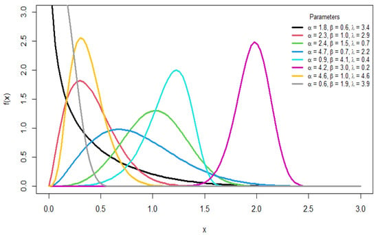
Figure 1.
Plots of the pdf for different parameter values.
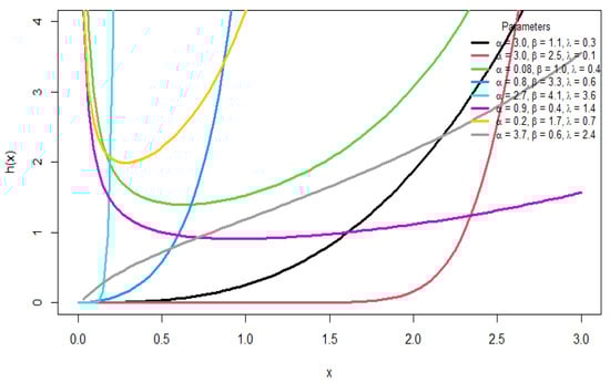
Figure 2.
Plots of the HRF for different parameter values.
Various shapes are shown in the pdf, including symmetric, left-skewed, right-skewed, and reverse J-shaped forms, whereas the hazard function provides different forms, such as increasing, bathtub, J-shaped, and reverse J-shaped forms. This illustrates the flexibility of the distribution in modeling different forms of data.
Special Cases of the NEW Distribution
It is noteworthy to mention that some well-known distributions are considered as special cases of the proposed distribution, such as the following:
- The exponentiated Gompertz distribution proposed by Ref. [8], when .
- The exponentiated Chen distribution introduced by Ref. [5], when .
- The odd Weibull Weibull distribution presented by Ref. [18], when .
- The odd generalized exponential Weibull distribution suggested by [19], when .
3. Mathematical Properties
3.1. Quantile Function
The quantile function for the NEW distribution is easily obtained by inverting the cdf in Equation (4), and is given by
3.2. Moments
The rth moment of a random variable X is a measure that gives information on a distribution’s shape and provides details of its central tendency and variations. Let X be a random variable with the pdf of the NEW distribution defined in Equation (3); then, the rth moment about the origin of X is given as
Using the binomial expansion
we obtain
We apply the following substitution:
Letting ⇒ we obtain
For r in general, Equation (8) can be solved numerically by applying statistical software for fixed values of the distribution’s parameters. When , the first moment about the origin is
For using the expansion
we obtain
3.3. Moment-Generating Function
The moment-generating function (MGF) is a method that is used to derive moments and understand the characteristics of a random variable for any distribution. The MGF is defined as
By substituting Equation (3) into Equation (11) and applying the binomial expansion in Equation (7), we have the following:
Let ⇒ Then,
3.4. Rényi Entropy
The entropy of a random variable X captures how much its uncertainty can vary. Let X be a random variable that follows the NEW distribution with the pdf defined in Equation (3). Then, the Rényi entropy can be obtained as follows:
Since , we apply the binomial expansion in Equation (7):
Therefore,
Let . Then, , and .
3.5. Order Statistics
4. Methods of Estimation
As part of assessing the efficiency of the NEW distribution, its parameters were estimated using different techniques, each with complementary advantages. These techniques included the maximum likelihood (ML) method, the least squares (LS) method, the Cramer–Von Mises (CVM) method, and the percentile (PE) method. These methods were chosen because they provide a comprehensive comparison of both distance- and likelihood-based estimation techniques.
4.1. Maximum Likelihood Method
The ML estimation is the most commonly utilized method of estimating the parameters in the statistical literature. It focuses on maximizing the log-likelihood function to obtain an estimate of the unknown parameters. Let be a sample obtained from the NEW distribution with parameters ; then, the log-likelihood function is given as
Therefore, an estimate of the distribution parameters can be obtained by taking the first derivative of Equation (18) with respect to each parameter as follows:
4.2. Least Squares Method
The LS method is one of the oldest estimation techniques, introduced in Ref. [39]. It estimates the parameters by minimizing the difference between the empirical and theoretical cdf. Let be the order statistics of a random sample from the NEW distribution; the least squares method aims to minimize the following objective function
Then, taking the first derivative of the objective function with respect to each parameter leads to the following:
4.3. Cramer–Von Mises Method
The CVM approach was formulated in Ref. [40] to estimate parameters by comparing the empirical and theoretical distribution functions in order to ensure an effective overall fit to the cdf. If is the order statistics of the random sample from the NEW distribution, the CVM method obtains an estimate of the parameters by minimizing the following equation:
Minimizing Equation (26) using a numerical optimization method or, alternatively, by solving the resulting equations gives the CVM estimates.
4.4. Percentile Method
The PE method was proposed in Ref. [41] as a simple estimation method. The PE approach compares the percentile points of the sample with their corresponding percentiles in the population by minimizing the Euclidean distance between them. In many scenarios, the PE estimators can be derived in a closed form, which makes it an attractive estimation method. For the order statistics obtained from a random sample from the NEW distribution, the PE approach aims to minimize the equation given below.
where is an estimate of . Similarly, percentile estimates are derived by minimizing Equation (30) or solving the following derivatives:
To obtain the estimates of the NEW distribution, the aforementioned methods were executed using the statistical software R (version 4.3.2). In particular, the optimization function optim with the Nelder–Mead algorithm was utilized to derive the estimates of the parameters.
5. Simulation
In an attempt to investigate the capability of the estimation methods in estimating the distribution parameters , simulation-based studies were conducted. By using the number of simulations and sample sizes of , the following three cases of the true value of the parameters were utilized:
As measures of accuracy, the bias and mean square error (MSE) were calculated for each estimate as follows:

Table 1.
Estimates, bias, and MSE of the parameters , and for case 1.
Table 2.
Estimates, bias, and MSE of the parameters , and for case 2.
Table 3.
Estimates, bias, and MSE of the parameters , and for case 3.
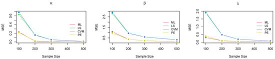
Figure 3.
Plot of the MSE for each parameter for all methods of estimation—case 1.
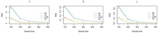
Figure 4.
Plot of the MSE for each parameter for all methods of estimation—case 2.
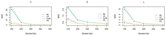
Figure 5.
Plot of the MSE for each parameter for all methods of estimation—case 3.
The above tables and figures show that, for small samples, the bias and MSE were high for all approaches, particularly for the parameter . For and , however, all methods performed better, with a slightly higher MSE for the ML method. As the sample size increased, there was a dramatic improvement in all the estimation methods, with a considerable reduction in both the bias and MSE for all parameters. By , the consistency property was achieved across all the estimation techniques, with a noticeable decrease in the MSE for all parameters. The ML method became much more stable, followed by the PE method. The LS and CVM methods were further enhanced with a high bias and MSE compared with ML and PE in most scenarios. Thus, they can be considered acceptable alternatives to the ML and PE approaches, despite being less efficient.
6. Application
For the purpose of assessing the distribution adequacy in fitting real data, seven statistical distributions were used. The considered distributions were the Weibull distribution along with six of its extensions that were built using different techniques. These Weibull-type extensions are widely employed in the literature due to their flexibility and applicability in modeling various forms of data. The aim was to investigate the flexibility of the NEW distribution compared with the Weibull distribution and its different extensions. The considered distributions were as follows:
- The Weibull (W) distribution:
- The exponentiated Weibull (EW) distribution [21]:
- The modified Weibull (MW) distribution [14]:
- The gull alpha-power Weibull (GAPW) distribution [20]:
- The generalized inverse Weibull (GIW) distribution [16]:
- The odd Weibull Weibull (OWW) distribution [18]:
- The KM exponentiated Weibull (KMEW) distribution [34]:
The comparison between the aforementioned distributions and the proposed NEW distribution was carried out using five different datasets to investigate the goodness of fit and adequacy in describing the data behavior.
6.1. Dataset Description
6.1.1. Dataset I: Blood Cancer Dataset
This dataset represents the lifetime, from diagnosis until death (in years), for 40 patients who suffered from blood cancer (leukemia). The data are complete (no censoring) and were provided by a hospital of the Ministry of Health in Saudi Arabia. The following data values have been used by many authors, such as Refs. [42,43,44]: 0.315, 0.496, 0.616, 1.145,1.208, 1.263, 1.414, 2.025, 2.036, 2.162, 2.211, 2.370, 2.532, 2.693, 2.805, 2.910, 2.912, 3.192, 3.263, 3.348, 3.348, 3.427, 3.499, 3.534, 3.767, 3.751, 3.858, 3.986, 4.049, 4.244, 4.323, 4.381, 4.392, 4.397, 4.647, 4.753, 4.929, 4.973, 5.074, 5.381. The data are summarized in Table 4.
Table 4.
Descriptive statistics for blood cancer data.
6.1.2. Dataset II: Single Carbon Fibers
The data are presented in Ref. [45] and contain tensile strength measurements in gigapascals (GPa) for single carbon fibers and impregnated bundles of 1000 fibers, tested at a gauge length of 20 mm. The dataset includes 69 recorded values as follows:
1.312, 1.314, 1.479, 1.552, 1.7, 1.803, 1.861, 1.865, 1.944, 1.958, 1.966, 1.997, 2.006, 2.021, 2.027, 2.055, 2.063, 2.098, 2.14, 2.179, 2.224, 2.24, 2.253, 2.27, 2.272, 2.274, 2.301, 2.301, 2.359, 2.382, 2.382, 2.426, 2.434, 2.435, 2.478, 2.49, 2.511, 2.514, 2.535, 2.554, 2.566, 2.57, 2.586, 2.629, 2.633, 2.642, 2.648, 2.684, 2.697, 2.726, 2.77, 2.773, 2.8, 2.809, 2.818, 2.821, 2.848, 2.88, 2.954, 3.012, 3.067, 3.084, 3.09, 3.096, 3.128, 3.233, 3.433, 3.585, 3.858. Table 5 provides a summary of the data.
Table 5.
Descriptive statistics for the single carbon fiber dataset.
6.1.3. Dataset III: Aircraft Windshield Dataset
This aircraft windshield dataset was used in Ref. [46] and represents the lifetimes of aircraft windshields (in units of 1000 h). A windshield is a multi-layered structure consisting of a strong outer skin and inner layers. If a malfunction of the heating system or the delamination of the outer ply occurs, a failure will occur and replacement of the windshield is required. The failure times for 63 aircraft windshields are as follows: 0.046, 1.436, 2.592, 0.140, 1.492, 2.600, 0.150, 1.580, 2.670, 0.248, 1.719, 2.717, 0.280, 1.794, 2.819, 0.313, 1.915, 2.820, 0.389, 1.920, 2.878, 0.487, 1.963, 2.950, 0.622, 1.978, 3.003, 0.900,2.053, 3.102, 0.952, 2.065, 3.304, 0.996, 2.117, 3.483, 1.003, 2.137, 3.500, 1.010, 2.141, 3.622,1.085, 2.163, 3.665, 1.092, 2.183, 3.695, 1.152, 2.240, 4.015, 1.183, 2.341, 4.628, 1.244, 2.435,4.806, 1.249, 2.464, 4.881, 1.262, 2.543, 5.140. Some descriptive statistics for the data are given in Table 6.
Table 6.
Descriptive statistics for the aircraft windshield dataset.
6.1.4. Dataset IV: Aluminum Fracture Toughness Dataset
This dataset denotes the fracture toughness of Aluminum2O3 and is reported in [47]. The values are as follows: 7.060066, 6.418242, 6.289877, 8.215349, 6.546606, 6.674971, 6.674971, 6.418242, 6.033147, 5.134593, 5.776417, 5.391323, 5.262958, 5.853436, 6.431078, 6.033147, 4.017819, 4.004983, 3.440177, 3.555706, 3.465850, 3.029410, 5.622380, 7.355305, 5.583870, 8.741645, 2.451768, 3.414504, 3.350322, 2.156529, 2.618643, 2.669988, 2.734171, 4.877864, 4.788008, 4.762335, 4.210366, 5.006228, 5.134593, 4.877864, 5.262958, 5.006228, 5.198776, 5.134593, 5.070411, 5.134593, 5.776417, 5.776417, 5.391323, 5.840600, 5.968965, 5.262958, 5.455505, 5.519688, 5.776417, 6.033147, 6.610789, 5.519688, 5.776417, 6.289877, 6.418242, 6.867518, 6.610789, 6.739154, 7.445160, 7.509343, 7.573525, 7.380978, 8.022802, 7.766072, 7.573525, 4.621134, 5.262958, 5.776417, 6.803336, 6.225694, 6.803336, 6.995883, 6.546606, 6.803336, 6.674971, 6.803336, 6.739154, 6.097329, 5.776417, 5.391323, 5.134593, 5.327140, 5.455505, 5.519688, 4.813681, 5.070411, 4.505606, 5.301467, 6.931701, 6.418242, 2.695661, 5.904782, 4.107675, 3.209121, 5.262958, 4.492769, 4.107675, 4.236039, 5.904782, 5.519688, 5.519688, 5.776417, 7.060066, 5.904782, 6.289877, 5.519688, 3.850945, 4.364404, 4.749499, 5.648053, 6.289877, 6.289877, 6.418242, 10.654281, 9.370633, 7.188430, 8.728808, 7.958619, 9.884092, 9.370633, 10.525916, 10.140822, 8.343714, 8.600444. Table 7 summarizes the data.
Table 7.
Descriptive statistics for the aluminum fracture toughness dataset.
6.1.5. Dataset V: Reliability Dataset
This dataset was presented in Ref. [48] and reported in Ref. [49], and it focuses on the failure and running times for a large system with 30 units. The values are as follows: 2.75, 0.13, 1.47, 0.23, 1.81, 0.30, 0.65, 0.10, 3.00,1.73, 1.06, 3.00, 3.00, 2.12, 3.00, 3.00, 3.00, 0.02, 2.61, 2.93, 0.88, 2.47, 0.28, 1.43, 3.00, 0.23, 3.00, 0.80, 2.45, 2.66. A summarization of this dataset is given in Table 8.
Table 8.
Descriptive statistics for the reliability dataset.
6.2. Distribution Comparison
This section compares the adequacy of the NEW distribution in fitting real data with the selected competitors by focusing on the relative performance with respect to goodness-of-fit indices and the predictive accuracy. The acquired information criteria are the following: the Akaike information criterion (AIC), Bayesian information criterion (BIC), Hannan–Quinn information criterion (HQIC), corrected Akaike information criterion (AICc), consistent Akaike information criterion (CAIC), and Kolmogorov–Smirnov (KS) test with its p-value. It is worth mentioning that the KS statistic is calculated using the estimated parameters; thus, its p-value should be interpreted as approximate. The utilization of these criteria is motivated by their distinct objectives and penalty structures, which allow for a more comprehensive model assessment. The results are shown in Table 9, Table 10, Table 11, Table 12 and Table 13 and Figure 6, Figure 7, Figure 8, Figure 9 and Figure 10.
Table 9.
The ML estimates with the standard error in parentheses and the goodness-of-fit measures for the blood cancer dataset.
Table 10.
The ML estimates with the standard error in parentheses and the goodness-of-fit measures for the single carbon fibers dataset.
Table 11.
The ML estimates with the standard error in parentheses and the goodness-of-fit measures for the aircraft windshield dataset.
Table 12.
The ML estimates with the standard error in parentheses and the goodness-of-fit measures for the aluminum fracture toughness dataset.
Table 13.
The ML estimates with the standard error in parentheses and the goodness-of-fit measures for the reliability dataset.
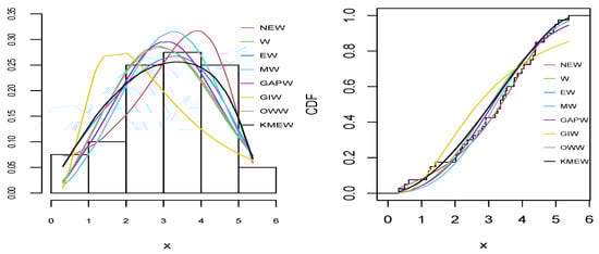
Figure 6.
The empirical pdf (right) and cdf (left) for all distributions for the blood cancer dataset.
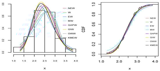
Figure 7.
The empirical pdf (right) and cdf (left) for all distributions for the single carbon fiber dataset.
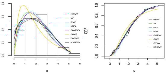
Figure 8.
The empirical pdf (right) and cdf (left) for all distributions for the aircraft windshield dataset.
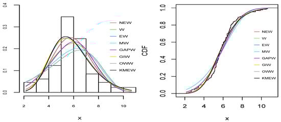
Figure 9.
The empirical pdf (right) and cdf (left) for all distributions for the aluminum fracture toughness dataset.
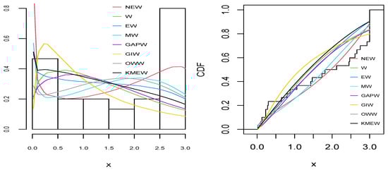
Figure 10.
The empirical pdf (right) and cdf (left) for all distributions for the reliability dataset.
As can be seen from Table 9, Table 10, Table 11, Table 12 and Table 13 and Figure 6, Figure 7, Figure 8, Figure 9 and Figure 10, the NEW distribution achieves a minimum value of all information criteria and a higher p-value among all distributions. This indicates the good ability of the NEW distribution to fit the data accurately compared with other extensions of the Weibull distribution.
7. Conclusions
Researchers’ interest in introducing new statistical distributions has resulted in an influx of data modeling in a wide range of applications. This study aimed to introduce a new, adaptable extension of the Weibull distribution by applying a logarithmic transformation to the exponentiated Weibull distribution. This new distribution, called the NEW distribution, has the ability to model different forms of pdfs and hazard functions, making it flexible in fitting complex behaviors. Some statistical properties of the NEW distribution were studied. Four estimation methods—the MLE, LS, CVM, and PE methods—were utilized to estimate the distribution parameters. Moreover, the efficiency of the estimation methods was compared using three simulation cases. The results demonstrated that the ML approach, followed by the PE method, achieved a higher accuracy in estimating the NEW parameters in comparison with the other methods. All the methods achieved the consistency property when the sample size increased. Additionally, five datasets were modeled with the NEW distribution and other formerly specified extensions of the Weibull distribution, and their results were compared. The obtained results evidenced that the NEW distribution is superior in terms of fitting the data; thus, it is considered a good alternative to other Weibull extensions in modeling various forms of data.
Although the present study indicates the applicability and usefulness of the proposed model, future research may be able to extend these findings in various directions. For example, using the penalized likelihood method or Bayesian technique with informative prior can help stabilize the estimators, especially in the case of small sample settings. Moreover, constructing a regression model for the NEW distribution would have considerable research value. Furthermore, the NEW distribution can be applied to censored data, which are popular in the fields of reliability engineering, economics, and finance.
Author Contributions
Conceptualization, D.A. and A.S.A.; methodology, D.A. and A.S.A.; software, D.A. and A.S.A.; validation, D.A. and A.S.A.; formal analysis, D.A. and A.S.A.; investigation, D.A. and A.S.A.; resources, D.A. and A.S.A.; data curation, D.A. and A.S.A.; writing—original draft preparation, D.A. and A.S.A.; writing—review and editing, D.A. and A.S.A.; visualization, D.A. and A.S.A. All authors have read and agreed to the published version of the manuscript.
Funding
This research received no external funding.
Data Availability Statement
The original contributions presented in this study are included in the article. Further inquiries can be directed to the corresponding author.
Conflicts of Interest
The authors declare no conflicts of interest.
References
- Marshall, A.W.; Olkin, I. A new method for adding a parameter to a family of distributions with application to the exponential and Weibull families. Biometrika 1997, 84, 641–652. [Google Scholar] [CrossRef]
- Gupta, R.C.; Gupta, P.L.; Gupta, R.D. Modeling failure time data by Lehman alternatives. Commun. Stat. Theory Methods 1998, 27, 887–904. [Google Scholar]
- Mahdavi, A.; Kundu, D. A new method for generating distributions with an application to exponential distribution. Commun. Stat.-Theory Methods 2017, 46, 6543–6557. [Google Scholar]
- Alzaatreh, A.; Lee, C.; Famoye, F. A new method for generating families of continuous distributions. Metron 2013, 71, 63–79. [Google Scholar] [CrossRef]
- Dey, S.; Kumar, D.; Ramos, P.L.; Louzada, F. Exponentiated Chen distribution: Properties and estimation. Commun. Stat.-Simul. Comput. 2017, 46, 8118–8139. [Google Scholar] [CrossRef]
- Ahmed, M.A. On the alpha power Kumaraswamy distribution: Properties, simulation and application. Rev. Colomb. Estad. 2020, 43, 285–313. [Google Scholar]
- Afify, A.Z.; Cordeiro, G.M.; Ibrahim, N.A.; Jamal, F.; Elgarhy, M.; Nasir, M.A. The Marshall-Olkin odd Burr III-G family: Theory, estimation, and engineering applications. IEEE Access 2020, 9, 4376–4387. [Google Scholar]
- Aslam, M.; Afzaal, M.; Bhatti, M.I. A study on exponentiated Gompertz distribution under Bayesian discipline using informative priors. Stat. Transit. New Ser. 2021, 22, 101–119. [Google Scholar] [CrossRef]
- İrhad, M.; Ahammed, E.M.; Maya, R.; Al-omari, A. Marshall-Olkin Bilal distribution with associated minification process and acceptance sampling plans. Hacet. J. Math. Stat. 2024, 53, 201–229. [Google Scholar] [CrossRef]
- Salahuddin, N.; Azeem, M.; Hussain, S.; Ijaz, M. A novel flexible TX family for generating new distributions with applications to lifetime data. Heliyon 2024, 10. [Google Scholar] [CrossRef] [PubMed]
- Alomair, A.M.; Ahmed, M.; Tariq, S.; Ahsan-ul Haq, M.; Talib, J. An exponentiated XLindley distribution with properties, inference and applications. Heliyon 2024, 10. [Google Scholar] [CrossRef]
- Namsaw, M.; Das, B.; Hazarika, P.J.; Alizadeh, M. The Alpha Power Modified Weibull-Geometric Distribution: A Comprehensive Mathematical Framework with Simulation, Goodness-of-fit Analysis and Informed Decision making using Real Life Data. Stat. Optim. Inf. Comput. 2025, 14, 1060–1087. [Google Scholar]
- Aliabadi, M.; Ghatari, A.H.; Khorram, E. A Three-Parameter Alpha Power Erlang Distribution for Modeling Lifetime Data. Stat. Optim. Inf. Comput. 2025. [Google Scholar]
- Lai, C.; Xie, M.; Murthy, D. A modified Weibull distribution. IEEE Trans. Reliab. 2003, 52, 33–37. [Google Scholar] [CrossRef]
- Cordeiro, G.M.; Ortega, E.M.; Nadarajah, S. The Kumaraswamy Weibull distribution with application to failure data. J. Frankl. Inst. 2010, 347, 1399–1429. [Google Scholar] [CrossRef]
- De Gusmao, F.R.; Ortega, E.M.; Cordeiro, G.M. The generalized inverse Weibull distribution. Stat. Pap. 2011, 52, 591–619. [Google Scholar] [CrossRef]
- Cordeiro, G.M.; Ortega, E.M.; Lemonte, A.J. The exponential–Weibull lifetime distribution. J. Stat. Comput. Simul. 2014, 84, 2592–2606. [Google Scholar] [CrossRef]
- Bourguignon, M.; Silva, R.B.; Cordeiro, G.M. The Weibull-G family of probability distributions. J. Data Sci. 2014, 12, 53–68. [Google Scholar] [CrossRef]
- Tahir, M.H.; Cordeiro, G.M.; Alizadeh, M.; Mansoor, M.; Zubair, M.; Hamedani, G.G. The odd generalized exponential family of distributions with applications. J. Stat. Distrib. Appl. 2015, 2, 1. [Google Scholar] [CrossRef]
- Ijaz, M.; Asim, S.M.; Alamgir; Farooq, M.; Khan, S.A.; Manzoor, S. A Gull Alpha Power Weibull distribution with applications to real and simulated data. PLoS ONE 2020, 15, e0233080. [Google Scholar] [CrossRef]
- Mudholkar, G.S.; Srivastava, D.K. Exponentiated Weibull family for analyzing bathtub failure-rate data. IEEE Trans. Reliab. 1993, 42, 299–302. [Google Scholar] [CrossRef]
- Pinho, L.; Cordeiro, G.; Nobre, J. The gamma-exponentiated Weibull distribution. J. Stat. Theory Appl. 2012, 11, 379–395. [Google Scholar]
- Eugene, N.; Lee, C.; Famoye, F. Beta-normal distribution and its applications. Commun. Stat.-Theory Methods 2002, 31, 497–512. [Google Scholar] [CrossRef]
- Mansour, M.; Korkmaz, M.Ç.; Ali, M.M.; Yousof, H.; Ansari, S.I.; Ibrahim, M. A generalization of the exponentiated Weibull model with properties, Copula and application. Eurasian Bull. Math. 2020, 3, 84–102. [Google Scholar]
- Ashraf, J.H.; Iqbal, Z.; Chakrabarty, T.K. A New Generalized Exponentiated Weibull Distribution: Properties and Applications. Thail. Stat. 2024, 22, 856–876. [Google Scholar]
- Kumar, D.; Singh, U.; Singh, S.K. A new distribution using sine function-its application to bladder cancer patients data. J. Stat. Appl. Probab. 2015, 4, 417. [Google Scholar]
- Kumar, D.; Singh, U.; Singh, S.K. A method of proposing new distribution and its application to Bladder cancer patients data. J. Stat. Appl. Pro. Lett. 2015, 2, 235–245. [Google Scholar]
- Maurya, S.K.; Kaushik, A.; Singh, R.K.; Singh, S.K.; Singh, U. A new method of proposing distribution and its application to real data. Imp. J. Interdiscip. Res. 2016, 2, 1331–1338. [Google Scholar]
- Kumar, D.; Singh, U.; Singh, U. Life time distributions: Derived from some minimum guarantee distribution. Sohag J. Math. 2017, 4, 7–11. [Google Scholar] [CrossRef]
- Kumar, D.; Kumar, P.; Kumar, P.; Singh, S.K.; Singh, U. PCM transformation: Properties and their estimation. J. Reliab. Stat. Stud. 2021, 14, 373–392. [Google Scholar] [CrossRef]
- Kavya, P.; Manoharan, M. Some parsimonious models for lifetimes and applications. J. Stat. Comput. Simul. 2021, 91, 3693–3708. [Google Scholar] [CrossRef]
- Dar, I.; Lone, M. A new class of probability distributions with an application in engineering science. Pak. J. Stat. Oper. Res. 2024, 20, 217–231. [Google Scholar] [CrossRef]
- Gauthami, P.; Chacko, V. Dus transformation of inverse Weibull distribution: An upside-down failure rate model. Reliab. Theory Appl. 2021, 16, 58–71. [Google Scholar]
- Alotaibi, N.; Elbatal, I.; Almetwally, E.M.; Alyami, S.A.; Al-Moisheer, A.; Elgarhy, M. Bivariate step-stress accelerated life tests for the Kavya–Manoharan exponentiated Weibull model under progressive censoring with applications. Symmetry 2022, 14, 1791. [Google Scholar] [CrossRef]
- Alotaibi, N.; Elbatal, I.; Shrahili, M.; Al-Moisheer, A.; Elgarhy, M.; Almetwally, E.M. Statistical inference for the Kavya–Manoharan Kumaraswamy model under ranked set sampling with applications. Symmetry 2023, 15, 587. [Google Scholar] [CrossRef]
- Afify, A.Z.; Abdelall, Y.Y.; AlQadi, H.; Mahran, H.A. The Modified Log-Logistic Distribution: Properties and Inference with Real-Life Data Applications. Contemp. Math. 2025, 790, 862–902. [Google Scholar] [CrossRef]
- West, R.M. Best practice in statistics: The use of log transformation. Ann. Clin. Biochem. 2022, 59, 162–165. [Google Scholar] [CrossRef]
- Curran-Everett, D. Explorations in statistics: The log transformation. Adv. Physiol. Educ. 2018, 42, 343–347. [Google Scholar] [CrossRef]
- Swain, J.J.; Venkatraman, S.; Wilson, J.R. Least-squares estimation of distribution functions in Johnson’s translation system. J. Stat. Comput. Simulation 1988, 29, 271–297. [Google Scholar] [CrossRef]
- Macdonald, P. Comments and Queries Comment on “An Estimation Procedure for Mixtures of Distributions” by Choi and Bulgren. J. R. Stat. Soc. Ser. B Stat. Methodol. 1971, 33, 326–329. [Google Scholar] [CrossRef]
- Kao, J.H. Computer methods for estimating Weibull parameters in reliability studies. IRE Trans. Reliab. Qual. Control 2009, PGRQC-13, 15–22. [Google Scholar] [CrossRef]
- Atallah, M.; Mahmoud, M.; Al-Zahrani, B. A new test for exponentiality versus NBUmgf life distributions based on Laplace transform. Qual. Reliab. Eng. Int. 2014, 30, 1353–1359. [Google Scholar] [CrossRef]
- Al-Saiary, Z.A.; Bakoban, R.A. The Topp-Leone generalized inverted exponential distribution with real data applications. Entropy 2020, 22, 1144. [Google Scholar] [CrossRef]
- Klakattawi, H.S. Survival analysis of cancer patients using a new extended Weibull distribution. PLoS ONE 2022, 17, e0264229. [Google Scholar] [CrossRef]
- Alrashidi, A. Arctan Kavya-Manoharan-G class of distributions with modelling in different fields. Adv. Appl. Stat. 2024, 91, 393–420. [Google Scholar] [CrossRef]
- Tahir, M.H.; Cordeiro, G.M.; Mansoor, M.; Zubair, M. The Weibull-Lomax distribution: Properties and applications. Hacet. J. Math. Stat. 2015, 44, 455–474. [Google Scholar] [CrossRef]
- Alshanbari, H.M.; Ahmad, Z.; El-Bagoury, A.A.A.H.; Odhah, O.H.; Rao, G.S. A new modification of the Weibull distribution: Model, theory, and analyzing engineering data sets. Symmetry 2024, 16, 611. [Google Scholar] [CrossRef]
- Meeker, W.; Escobar, L. Statistical Methods for Reliability Data; John Wiley & Sons: New York, NY, USA, 1998. [Google Scholar]
- Klakattawi, H.S.; Aljuhani, W.H.; Baharith, L.A. Alpha power exponentiated new Weibull-Pareto distribution: Its properties and applications. Pak. J. Stat. Oper. Res. 2022, 18, 703–720. [Google Scholar] [CrossRef]


Disclaimer/Publisher’s Note: The statements, opinions and data contained in all publications are solely those of the individual author(s) and contributor(s) and not of MDPI and/or the editor(s). MDPI and/or the editor(s) disclaim responsibility for any injury to people or property resulting from any ideas, methods, instructions or products referred to in the content. |
© 2025 by the authors. Licensee MDPI, Basel, Switzerland. This article is an open access article distributed under the terms and conditions of the Creative Commons Attribution (CC BY) license (https://creativecommons.org/licenses/by/4.0/).