
Piecewise Analytical Approximation Methods for Initial-Value Problems of Nonlinear Ordinary Differential Equations


Abstract
:1. Introduction
2. Piecewise Continuous Solutions Based on Quadratic Approximations
2.1. Piecewise Continuous Solutions of the Generalized Riccati Equation (2) for
2.2. Piecewise Continuous Solutions of the Generalized Riccati Equation (2) for
3. Piecewise Continuous Solutions Based on Quadratic Approximations with Frozen Coefficients
3.1. Piecewise Continuous Solutions for
3.2. Piecewise Continuous Solutions for
4. Discrete Mappings/Finite-Difference Techniques for Piecewise Continuous Methods Based on Quadratic Approximations
5. Discrete Methods Based on Quadratic Approximations
5.1. Discrete Methods Based on Quadratic Approximations for
5.2. Discrete Methods Based on Quadratic Approximations for and
6. Discrete Methods Based on Frozen-Coefficient Approximations
7. Results
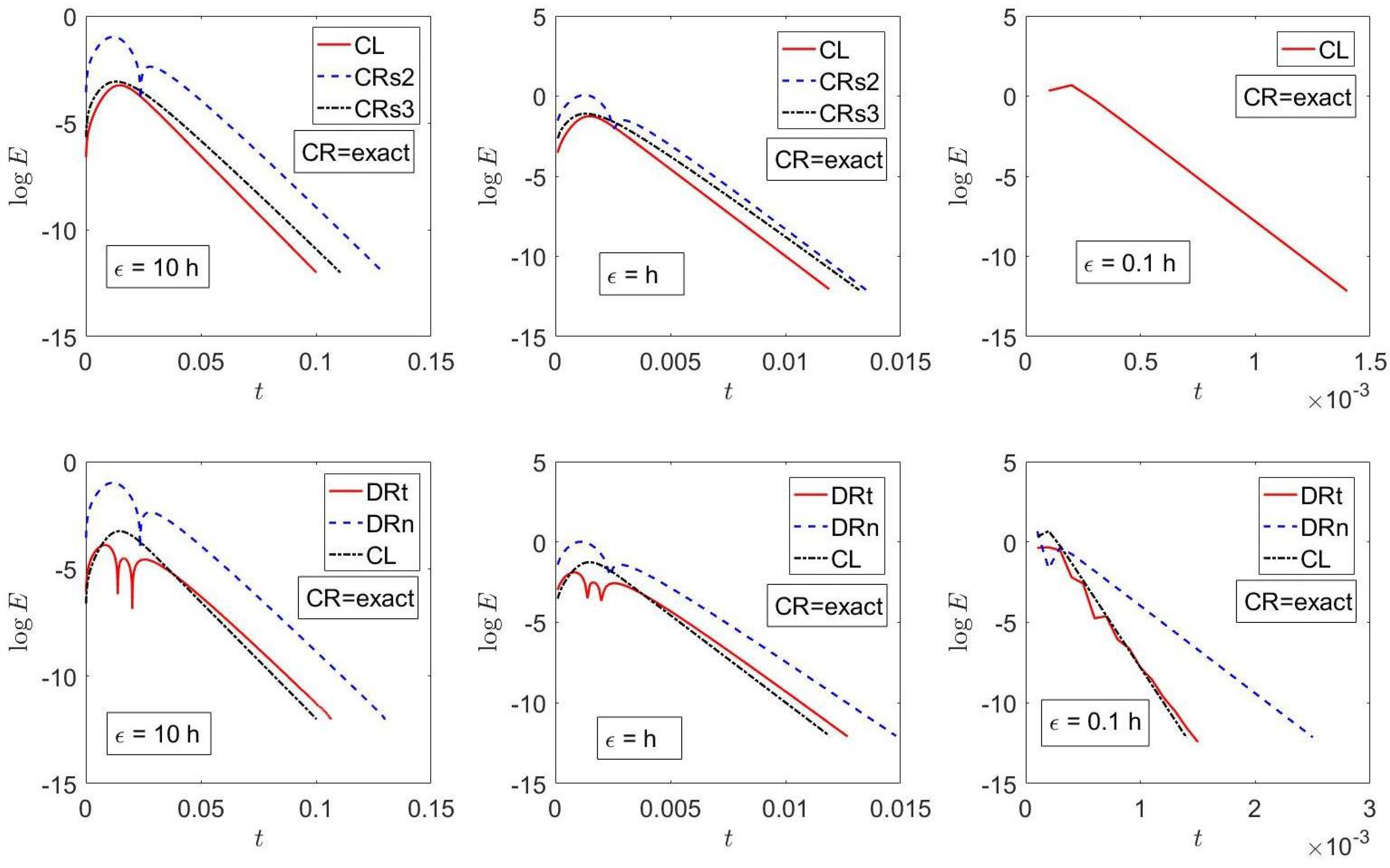
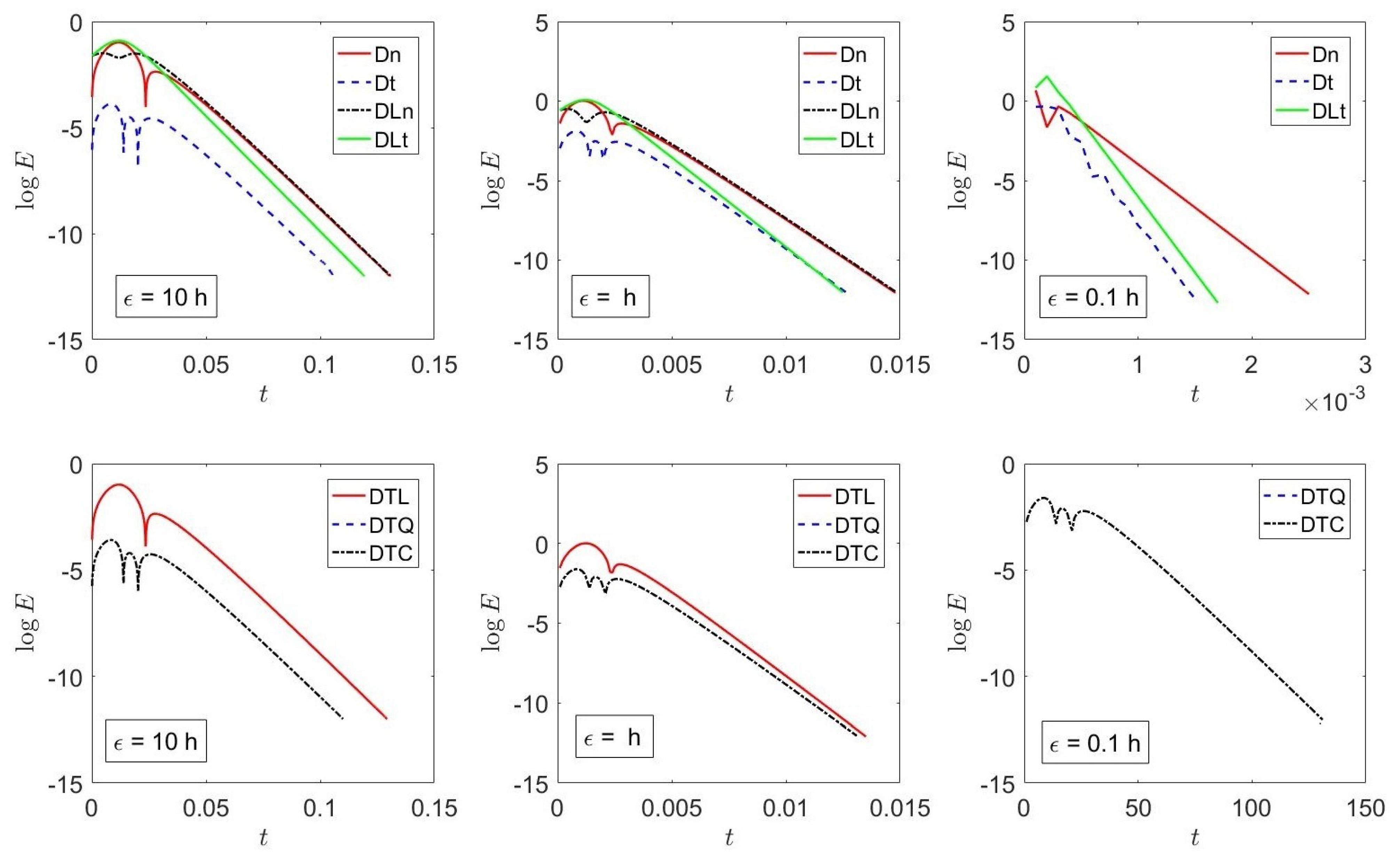
7.1. Example 1
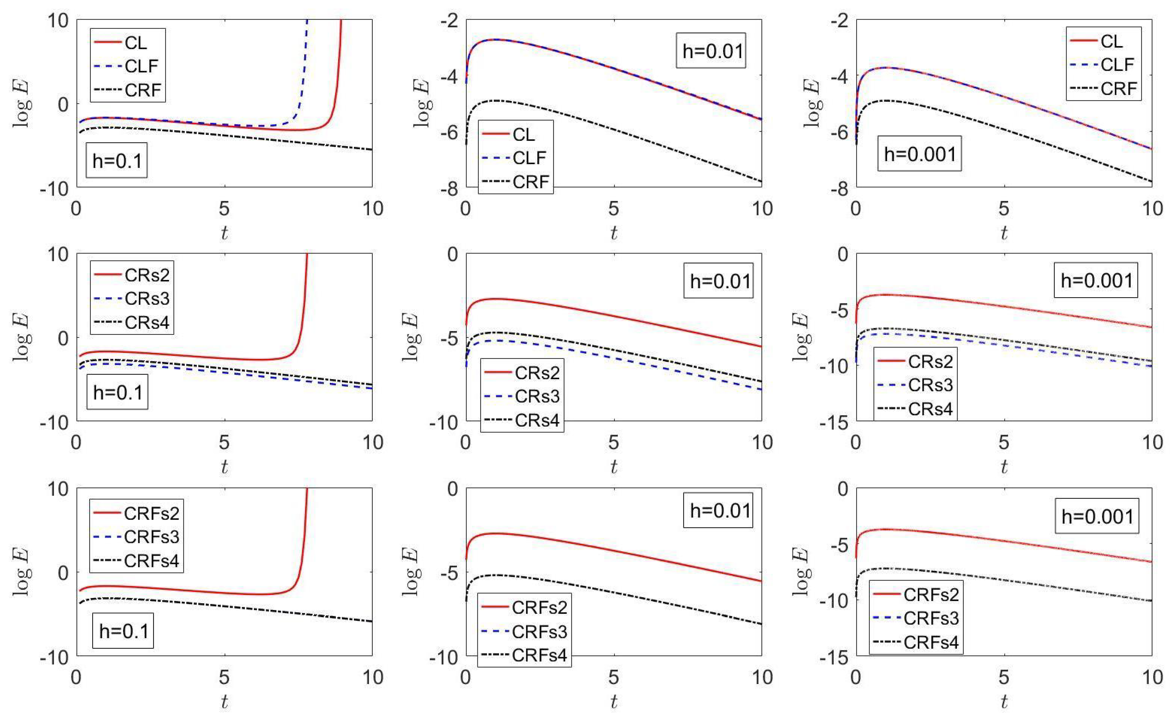
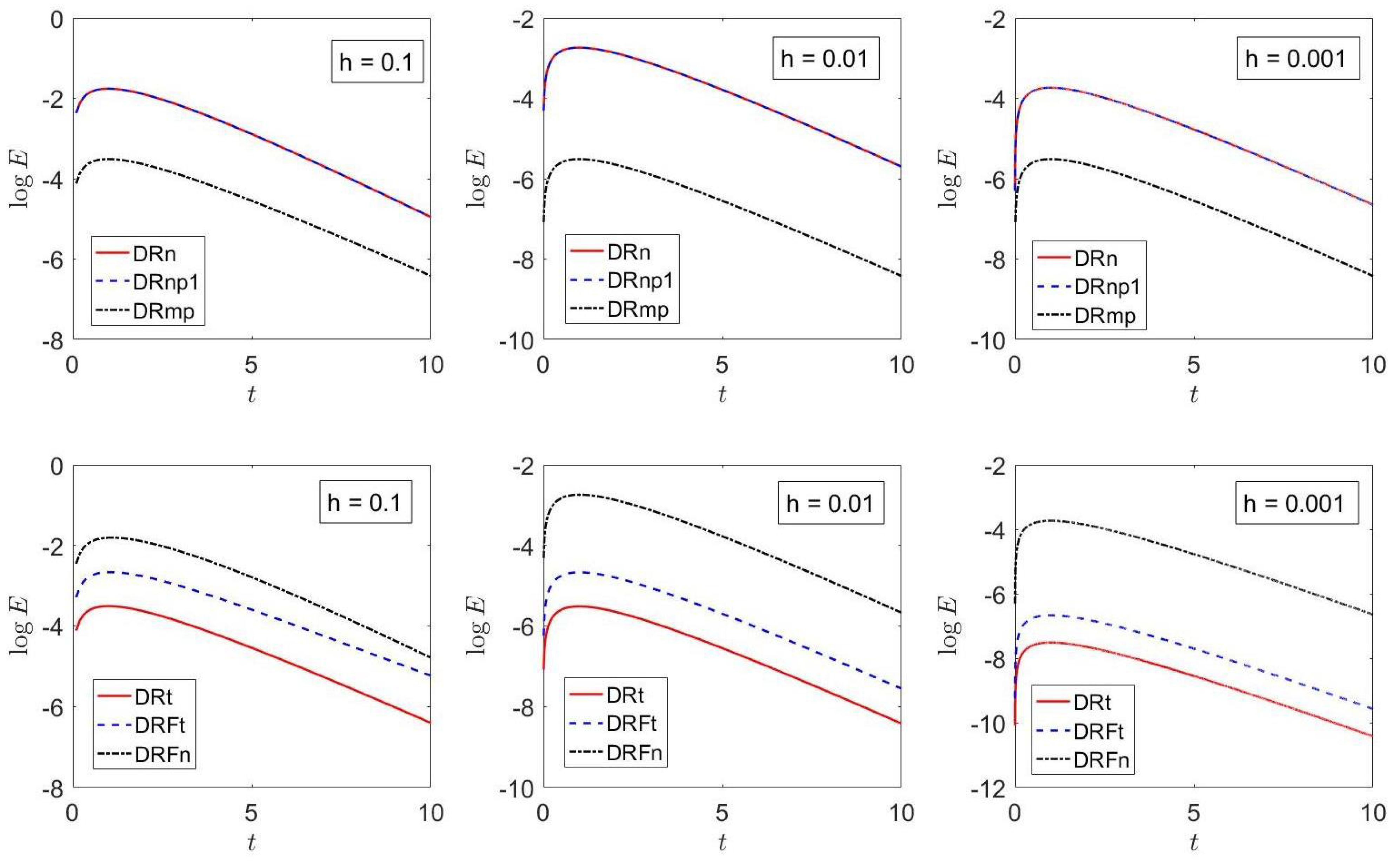
7.2. Example 2
8. Conclusions
Funding
Data Availability Statement
Acknowledgments
Conflicts of Interest
Appendix A. Piecewise Continuous Methods Based on Linear Approximations
Appendix B. Discrete Methods Based on Linear Approximations
Appendix C. Taylor’s Methods
References
- Tan, Z.; Su, G.; Su, J. Improved lumped models for combined convective and radiative cooling of a wall. Appl. Therm. Eng. 2009, 29, 2439–2443. [Google Scholar] [CrossRef]
- Su, G.; Tan, Z.; Su, J. Improved lumped models for transient heat conduction in a slab with temperature–dependent thermal conductivity. Appl. Math. Model. 2009, 33, 274–283. [Google Scholar] [CrossRef]
- Alhama, F.; Zueco, J. Application of a lumped model to solids with temperature–dependent thermal conductivity. Appl. Math. Model. 2007, 31, 302–310. [Google Scholar] [CrossRef]
- Sahu, S.K.; Behera, P. An improved lumped analysis for transient heat conduction in different geometries with heat generation. C. R. Mec. 2012, 340, 477–484. [Google Scholar] [CrossRef]
- Shitzer, A.; Stroschein, L.A.; Gonzalez, R.R.; Pandolf, K.B. Lumped–parameter tissue temperature–blood perfusion model of a cold-stressed fingertip. J. Appl. Physiol. 1996, 80, 1829–1834. [Google Scholar] [CrossRef] [PubMed]
- Gao, Y.; Shan, R.; Lyra, S.; Li, C.; Wang, H.; Chen, J.H.; Lu, T. On lumped-reduced reaction model for combustion of liquid fuels. Combust. Flame 2016, 163, 437–446. [Google Scholar] [CrossRef]
- Ranzi, E.; Dente, M.; Goldaniga, A.; Bozzano, G.; Faravelli, T. Lumping procedures in detailed kinetic modeling of gasification, pyrolysis, partial oxidation and combustion of hydrocarbon mixtures. Prog. Energy Combust. Sci. 2001, 27, 99–139. [Google Scholar] [CrossRef]
- Ramos, J.I. Lumped models of gas bubbles in thermal gradients. J. Appl. Math. Model. 1997, 21, 371–386. [Google Scholar] [CrossRef]
- Ramos, J.I. Multicomponent Gas Bubbles. II. Bubble Dynamics. J. Non-Equilib. Thermodyn. 1988, 13, 107–131. [Google Scholar] [CrossRef]
- Abramowitz, M.; Stegun, I.A. (Eds.) Handbook of Mathematical Functions with Formulas, Graphs, and Mathematical Tables, 9th ed.; Dover: New York, NY, USA, 1972. [Google Scholar]
- Zwillinger, D. Handbook of Differential Equations, 3rd ed.; Academic Press: New York, NY, USA, 1997. [Google Scholar]
- Polyanin, A.D.; Zaitsev, V.F. Handbook of Exact Solutions for Ordinary Differential Equations, 2nd ed.; Chapman & Hall/CRC Press: New York, NY, USA, 2003. [Google Scholar]
- Murphy, G.M. Ordinary Differential Equations and Their Solutions; Dover: New York, NY, USA, 2011. [Google Scholar]
- Pope, D.A. An exponential method of numerical integration of ordinary differential equations. Commun. ACM 1963, 6, 491–493. [Google Scholar] [CrossRef]
- Ramos, J.I. Linearization techniques for singularly–perturbed initial–value problems of ordinary differential equations. Appl. Math. Comput. 2005, 163, 1143–1163. [Google Scholar] [CrossRef]
- De la Cruz, H.; Bisccay, R.J.; Carbonell, F.; Ozaki, T.; Jimenez, J.C. A higher order linearization method for solving ordinary differential equations. Appl. Math. Comput. 2007, 185, 197–212. [Google Scholar] [CrossRef]
- Hochbruck, M.; Ostermann, A. Exponential integrators. Acta Numer. 2010, 19, 209–286. [Google Scholar] [CrossRef]
- Chu, S.C.; Berman, M. An exponential method for the solution of systems of ordinary differential equations. Commun. ACM 1974, 17, 699–702. [Google Scholar] [CrossRef]
- Guderley, K.G.; Hsu, C.-C. A predictor–corrector method for a certain class of stiff differential equations. Math. Comput. 1972, 26, 51–69. [Google Scholar] [CrossRef]
- Boyle, P.P.; Tian, W.; Guan, F. The Riccati equation in mathematical finance. J. Symb. Comput. 2002, 33, 343–355. [Google Scholar] [CrossRef]
- Kovacic, J.J. An algorithm for solving second order linear homogeneous differential equations. J. Symb. 1986, 2, 3–43. [Google Scholar] [CrossRef]
- Bittani, S.; Laub, A.J.; Willems, J.C. (Eds.) The Riccati Equation; Springer: Berlin, Germany, 1991. [Google Scholar]
- Jungers, M. Historical perspectives of the Riccati equation. IFAC-PapersOnLine 2017, 50, 9535–9546. [Google Scholar] [CrossRef]
- Lagrange, R. Quelques théorèmes d’integrabilité par quadratures de l’équation de Riccati. Bull. Soc. Math. Fr. 1938, 66, 155–163. [Google Scholar] [CrossRef]
- Haley, S.B. An underrated entanglement: Riccati and Schrödinger equations. Am. J. Phys. 1997, 65, 237–243. [Google Scholar] [CrossRef]
- Al Bastami, A.; Belić, M.R.; Petrović, N.Z. Special solutions of the Riccati equation with applications to the Gross–Pitaevskii nonlinear pde. Electron. J. Differ. 2010, 66, 1–10. [Google Scholar]
- Kudryashov, N.A.; Sinelshchikov, D. Comment on ‘Exact solutions to the various nonlinear evolution equations’. Phys. Scr. 2011, 83, 017001. [Google Scholar] [CrossRef]
- Clarkson, J. Painlevé equations–Nonlinear special functions. In Orthogonal Polynomials and Special Functions: Computation and Application; Marcellán, F., van Assche, W., Eds.; Lecture Notes in Mathematics; Springer: Berlin, Germany, 2006; Volume 1883, pp. 331–411. [Google Scholar]
- Olver, F.W.J.; Lozier, D.W.; Boisvert, R.F.; Clark, C.W. (Eds.) NIST Handbook of Mathematical Functions; Cambridge University Press: New York, NY, USA, 2020. [Google Scholar]
- Euler, M.; Euler, N.; Leach, P. The Riccati and Ermakov–Pinney hierarchies. J. Nonlinear Math. Phys. 2007, 14, 290–310. [Google Scholar] [CrossRef]
- Musette, M. Painlevé analysis for nonlinear partial differential equations. In The Painlevé Property: One Century Later; Conte, R., Ed.; Springer: New York, NY, USA, 1999; pp. 517–572. [Google Scholar]
- Conte, R.; Musette, M. The Painlevé Handbook, 2nd ed.; Springer: New York, NY, USA, 2008. [Google Scholar]
- Ince, E.L. Ordinary Differential Equations; Dover: New York, NY, USA, 1956. [Google Scholar]
- Davis, H.T. Introduction to Nonlinear Differential and Integral Equations; Dover: New York, NY, USA, 1962. [Google Scholar]
- Reid, W.T. Riccati Differential Equations; Academic Press: New York, NY, USA, 1972. [Google Scholar]
- Glaisher, J.W.L. On Riccati’s Equation. Q. J. Pure Appl. Math. 1871, 11, 267–273. [Google Scholar]
- Bender, C.M.; Orszag, S.A. Advanced Mathematical Methods for Scientists and Engineers; McGraw-Hill: New York, NY, USA, 1978. [Google Scholar]
- Dawson, H.G. On the numerical value of dx. Proc. Lond. Math. Soc. 1897, s1–29, 519–522. [Google Scholar] [CrossRef]
- Spanier, J.; Oldham, K.B. An Atlas of Functions; Hemisphere: Washington, DC, USA, 1987. [Google Scholar]
- Luke, Y.L. The Special Functions and Their Approximations; Academic Press: New York, NY, USA, 1969; Volume 2. [Google Scholar]
- Press, W.H.; Flannery, B.P.; Teukolsky, S.A.; Vetterling, W.T. Numerical Recipes: The Art of Scientific Computing, 3rd ed.; Cambridge University Press: Cambridge, UK, 2007. [Google Scholar]
- Certaine, J. The solution of ordinary differential equations with large time constants. In Mathematical Methods for Digital Computers; Ralston, A., Wilf, S., Eds.; John Wiley & Sons: New York, NY, USA, 1965; pp. 128–132. [Google Scholar]

| Method | Sect/App | () | () | () |
|---|---|---|---|---|
| CR | Section 4 | |||
| CRF | Section 4 | |||
| CRs2 | Section 4 | −0.978 | +0.064 | Diverges |
| CRs3 | Section 4 | −3.073 | −1.098 | Diverges |
| CL | Appendix A | −3.245 | −1.256 | +0.681 |
| DRtn | Section 5.1 | −3.884 | −1.886 | −0.365 |
| DRn | Section 5.1 | −0.984 | +0.018 | −0.984 |
| Dtn | Section 5 | −3.586 | −1.886 | −0.327 |
| Dn | Section 5 | −0.984 | +0.018 | +0.683 |
| DLn | Appendix B | −1.492 | −0.499 | Diverges |
| DLtn | Appendix B | −0.906 | −0.070 | +1.553 |
| DTL | Appendix C | −0.984 | +0.011 | Diverges |
| DTQ | Appendix C | −3.589 | −1.611 | Diverges |
| DTC | Appendix C | −3.589 | −1.611 | Diverges |
| Method | Sect/App | () | () | () |
|---|---|---|---|---|
| CRF | Section 4 | −6.911 | −4.909 | −2.890 |
| CRs2 | Section 4 | −3.735 | −2.733 | Diverges |
| CRs3 | Section 4 | −7.212 | −5.209 | −3.180 |
| CRs4 | Section 4 | −6.735 | −4.731 | −2.696 |
| CRFs2 | Section 4 | −3.735 | −2.733 | Diverges |
| CRFs3 | Section 4 | −7.212 | −5.207 | −3.158 |
| CRFs4 | Section 4 | −7.212 | −5.207 | −3.159 |
| CL | Appendix A | −3.735 | −2.735 | −1.731 |
| CLF | Appendix A | −3.735 | −2.733 | Diverges |
| DRt | Section 5.1 | −7.513 | −5.513 | −3.507 |
| DRFt | Section 6 | −6.668 | −4.668 | −2.663 |
| DRn | Section 5.1 | −3.736 | −2.739 | −1.761 |
| DRFn | Section 6 | −3.736 | −2.742 | −1.808 |
| DRmp | Section 5.1 | −7.514 | −5.513 | −3.513 |
| DRnp1 | Section 5.1 | −3.736 | −2.738 | −1.760 |
| DLt | Section 6 | −7.513 | −5.513 | −3.514 |
| DLFt | Section 6 | −7.513 | −5.513 | −3.493 |
| DLnp1 | Section 6 | −3.735 | −2.729 | −1.682 |
| DLn | Section 6 | −3.736 | −2.738 | −1.762 |
| DLFn | Section 6 | −3.735 | −2.734 | −1.720 |
| DLmp | Section 6 | −7.212 | −5.212 | −3.214 |
Disclaimer/Publisher’s Note: The statements, opinions and data contained in all publications are solely those of the individual author(s) and contributor(s) and not of MDPI and/or the editor(s). MDPI and/or the editor(s) disclaim responsibility for any injury to people or property resulting from any ideas, methods, instructions or products referred to in the content. |
© 2025 by the author. Licensee MDPI, Basel, Switzerland. This article is an open access article distributed under the terms and conditions of the Creative Commons Attribution (CC BY) license (https://creativecommons.org/licenses/by/4.0/).
Share and Cite
Ramos, J.I. Piecewise Analytical Approximation Methods for Initial-Value Problems of Nonlinear Ordinary Differential Equations. Mathematics 2025, 13, 333. https://doi.org/10.3390/math13030333
Ramos JI. Piecewise Analytical Approximation Methods for Initial-Value Problems of Nonlinear Ordinary Differential Equations. Mathematics. 2025; 13(3):333. https://doi.org/10.3390/math13030333
Chicago/Turabian StyleRamos, Juan I. 2025. "Piecewise Analytical Approximation Methods for Initial-Value Problems of Nonlinear Ordinary Differential Equations" Mathematics 13, no. 3: 333. https://doi.org/10.3390/math13030333
APA StyleRamos, J. I. (2025). Piecewise Analytical Approximation Methods for Initial-Value Problems of Nonlinear Ordinary Differential Equations. Mathematics, 13(3), 333. https://doi.org/10.3390/math13030333