Abstract
Zero-shot learning (ZSL) holds significant promise for scaling image classification to previously unseen classes by leveraging previously acquired knowledge. However, conventional ZSL methods face challenges such as domain-shift and hubness problems. To address these issues, we propose a novel kernelized similarity learning approach that reduces intraclass similarity while increasing interclass similarity. Specifically, we utilize kernelized ridge regression to learn visual prototypes for unseen classes in the semantic vectors. Furthermore, we introduce kernel polarization and autoencoder structures into the similarity function to enhance discriminative ability and mitigate the hubness and domain-shift problems. Extensive experiments on five benchmark datasets demonstrate that our method outperforms state-of-the-art ZSL and generalized zero-shot learning (GZSL) methods, highlighting its effectiveness in improving classification performance for unseen classes.
MSC:
68T10; 68T45; 62J07
1. Introduction
With the daily increase in novel categories of objects in nature, such as new species of fish and birds, it is essential to construct classification models for these new categories. In the context of traditional models, the quality of classification is contingent on the availability of a sufficient number of instances of each class for the purpose of training. However, this is not a viable option for non-trained classes. In addition to the necessity of collecting large amounts of data for new categories, the subsequent annotation of these data represents a significant expense. Furthermore, the construction of a new training set and the retraining of the model are required for each new category added to the dataset, which can be impractical. To address these problems, ref. [1] presented for the first time a method called zero-shot learning to discriminate instances that do not participate in training, thus improving the generalizability of classification models.
ZSL relates new category instances to known category instances using semantic information, e.g., describing a zebra (assuming it is an unknown animal) with “it is shaped like a horse and colored like a panda”. Such data can be obtained in several ways, including the use of manually defined semantic attributes to describe the semantic features of instances [1,2] or vector embeddings of class names through related models [3]. In both approaches, a feature vector is used to describe the semantic information of each class, and the composed space becomes the semantic space. Each category in this space has only one vector to represent the features, unlike the visual feature space, where each instance of each category is represented by a visual feature vector. Semantic vectors for seen and unseen classes are always available for training or testing, but only seen class instances are involved in training. The objective of the ZSL approach is to discover relationships between classes to construct a knowledge migration system from the implicit relationships in seen and unseen classes to match semantic features and visual features of unseen classes.
The traditional ZSL model is based on the assumption that only instances of the unseen class are involved during the testing phase. Consequently, the classification is performed exclusively in the unseen class. However, in practice, the true class should be recognized among all classes, based on the more reasonable assumption that both seen and unseen classes participate in the testing phase. This approach is called generalized zero-shot learning (GZSL) [4].
From a methodological viewpoint, there are currently three dominant approaches in ZSL: (1) global compatibility methods, (2) embedding space methods, and (3) generative methods [5]. The global compatibility approach [6,7] involves defining a global compatibility function on visual feature vectors and semantic vectors, whose goal is to maximize the compatibility score of the correct class of semantic vectors with each training instance. The embedding space approach maps visual feature vectors to the semantic space, maps them in the opposite direction, or maps both to a predefined common space. Once the different features have been mapped to the same space, the maximum similarity, which is typically the closest distance, is then used to match instances and categories. Some studies [8,9] map visual feature vectors to the semantic space to preserve the semantic structure. In contrast, other studies [10,11] change the embedding direction to form unique visual prototypes. A final trend in embedding approaches is to unify the visual feature vectors and corresponding semantic feature vectors by defining a projection function that maps them into a common space [12]. The generic approach [13,14] re-samples each learned class by analyzing the connection between seen and unseen classes in conjunction with semantic relations [5]. Then, enough instances of the unseen classes are generated to join the training, thus transforming ZSL into a traditional classification task. Generative networks, such as Generative Adversarial Networks (GANs) [15,16,17], are often used to achieve this goal. Generative models are larger in time and space complexity than the other two methods, with lower visibility and interaction. This paper focuses on the embedding space approach.
There is a problem in ZSL called the domain-shift problem (DSP), where the apparent difference in the distribution of data in the source (training) and target (test) domains can lead to a bias toward the seen classes, thus preventing the model from achieving reasonable recognition performance [18]. To address this problem, some researchers consider unseen class instances as negative samples in the training phase, in addition to labeled seen class instances, instead of adhering to the inductive setting of ZSL, which is called transductive ZSL [19]. However, in realistic recognition scenarios, data related to unobserved classes are usually not available during training. Therefore, the transductive setting is rarely considered the best solution to the DSP.
Another challenge in ZSL is called the hubness problem [20]. Hubness arises when points are randomly selected in a high-dimensional space, as there is a tendency for some points to frequently appear in the neighborhood of other points, which means that when using nearest neighbor searches, such points are often retrieved [21]. For ZSL methods that map visual features into the semantic space, hubness is observed in classification since this embedding direction is usually in a high-dimensional space. To mitigate this problem, several methods attempt to learn appropriate distance functions with parameters, instead of using general distance metrics such as Euclidean distance [10,22]. However, disjoining the training and test classes still degrades the classification ability of the model.
To address the above problems, this paper proposes a similarity learning algorithm using the kernel of the embedding space method, which aims to increase the similarity between instances and visual prototypes of the same class while decreasing the similarity with visual prototypes of different classes. For the construction of category-specific prototypes, kernelized ridge regression is proposed for learning visual prototypes in their semantic vectors. Applications of kernelization have demonstrated the potential to enhance model generalization; however, this avenue has rarely been explored in ZSL and GZSL. In addition, kernel polarization is applied to the kernelized similarity function to improve the classification ability of the model, and autoencoder structures are introduced into the optimization objective function to reduce hubness and the DSP. The classification performance of the model is evaluated on five standard datasets in both ZSL and GZSL experiments. The results show that the classification ability of the model is improved compared to other methods. Our contributions are as follows:
- A kernelized similarity function is proposed to adjust the cosine distance of visual feature vectors to associated prototypes mapped into the visual feature space, alleviating hubness and the DSP.
- The similarity function is enhanced using the kernel polarization method to improve discriminative ability.
- A prototype learning method based on kernelized ridge regression is used to represent unseen visual prototypes.
2. Related Works
In this section, we present related works on prototype learning, followed by some advances in distance learning. In Table 1, the proposed method is compared to related works based on various criteria.
2.1. Prototype Learning
Prototype learning is a prevalent model in embedding methods that prioritizes the construction of prototypes for unseen classes. These approaches minimize the intraclass distance between visual instances and related class prototypes as an optimization goal to mitigate hubness so that nearest neighbor search is not greatly affected. The authors of [23] converted the embedding direction, and the proposed method follows this idea by constructing a nonlinear function to project semantic features onto the visual feature space and minimizing the intraclass distances between the projection vectors and the feature vectors of instances of the same class to obtain the visual prototype. The authors of [24] employed the class average of the visual instances as the visual prototype, subsequently solving for the projection matrix of the semantic features mapped to the visual prototype.
The two aforementioned methods are two directions for acquiring visual prototypes. The method in [23], where the prototype is uncertain and is learned by minimizing the distance between the seen class and the intraclass, is called early learning. The method in [24], where the prototype is deterministic and is the mean of the seen class instances, is called late learning. Section 3 demonstrates that these two learning methods yield consistent results if the objective function is set to the mean square error and the mapping method is set to linear mapping.
Inspired by the above methods, this paper uses a prototype learning method to obtain visual prototypes, and in particular, kernelized ridge regression is used as the learning method. After obtaining the visual prototype, a discriminative method is also needed. In this paper, the kernelized similarity function is constructed for classification instead of Euclidean distance.
2.2. Distance Learning
Recently, distance learning has been considered a useful approach to improve the classification ability of ZSL instead of using traditional distance functions. In embedding space methods based on learning mapping functions, the use of appropriate metrics can clearly distinguish between instances of different classes and alleviate hubness. The authors of [25] proposed a Mahalanobis metric learning method in the form of a parameterized Gaussian distribution with a common covariance matrix shared by all classes and class-specific means. While that study considered one-shot learning, [26] proposed a model based on class-specific Gaussian distributions. This model differs from the model in [25] in whether the learned covariance matrix is shared.
In [22], Bucher et al. adopted a learning approach based on Euclidean distance for ZSL to develop a distance function that more accurately predicts the congruence between an embedded image and its associated semantic vectors. To achieve this objective, the visual feature embedding learns a normalized affine function with ReLU form via a least squares objective function. In [25,26], while the distance function is also learned, the authors concentrated on minimizing the distance between visual instances and related prototypes. In contrast, [22] aimed to identify suitable distance functions between visual instances and their associated prototypes.
In recent years, in addition to distance functions based on the Mahalanobis and Euclidean metrics, researchers have explored other types of distance functions. For example, in [10], researchers proposed a distance function based on cosine similarity to measure the relationship between a specific class of prototypes and instances. This approach employs semantic feature vectors as inputs to construct visual prototypes through the use of multilayer neural network models.
Although mitigating hubness and the DSP in ZSL and GZSL by learning distance functions is an effective approach, these methods still suffer from the DSP due to inconsistencies in the distribution of unseen classes. One of the main contributions of this paper is to extend the distance function using an autoencoder structure to ensure that its original structure is maintained when semantic features are embedded in the visual feature space, thus mitigating the DSP. Furthermore, while learning the distance function, we introduce a kernel polarization method similar to large marginal loss to optimize both structural and empirical risk.

Table 1.
Differences between the proposed method and related works based on various criteria.
Table 1.
Differences between the proposed method and related works based on various criteria.
| Method | Category | Target Space | Focus | Early/Late Learning | Kernel |
|---|---|---|---|---|---|
| Zhang et al. [23] | embedding space | visual | distance | early | no |
| Changpinyo et al. [24] | embedding space | visual | distance | late | yes |
| Jiang et al. [4] | embedding space | visual/semantic/third | distance | early | no |
| Verma and Rai [26] | embedding space | visual | distance | late | no |
| Pan et al. [10] | embedding space | visual | similarity | early | no |
| Zhang and Koniusz [27] | embedding space | semantic | similarity | - | yes |
| Our Method | embedding space | visual | similarity | late | yes |
3. Background
stands for the index set . Let and be the data matrices that contain N column vectors and for . is the norm of the matrix X.
Proposition 1
(Autoencoder structure). Assume that W is a transformation matrix from Y to X and l is a loss function. Then, the following expression is called the autoencoder structure:
Minimizing L promotes a weak incoherence between the column vectors of W.
Proof.
For brevity, we do not consider the specific form of the loss function. Let the approximation error matrices be and , e.g., and . Combining both, we obtain
where stands for the total approximation error matrix. If , then . This means that the lower the error, the more independent the components become. In particular, if , then W is an orthogonal matrix. □
Proposition 2
(Kernel alignment [28]). Let and be two positive (semi)definite kernel functions. Assume that denote two Gram matrices that are generated by applying the kernel functions k and to X and Y, respectively. Then, the empirical alignment of two kernels is also a positive (semi)definite kernel, and its value is given by the dot product between K and :
Proof.
Mercer theorem [29] states that the feature mappings and correspond to the kernels k and , respectively. For any ,
Therefore, Equation (3) is a positive (semi)definite kernel. □
Proposition 3
(Kernel polarization [28]). Let be a positive (semi)definite kernel function. Assume that denotes the Gram matrix of k applied to X. Moreover, let each column vector of X have a corresponding label for such that X has a corresponding label vector . is a rank-1 kernel. Then, the empirical alignment of K and L forms a positive semidefinite kernel, which is called kernel polarization:
Proof.
Since L is a rank-1 matrix and the diagonal elements are 1, L is a positive semidefinite kernel. Furthermore, since K is a positive (semi)definite kernel, the conclusion holds using Proposition 2. □
4. Proposed Method
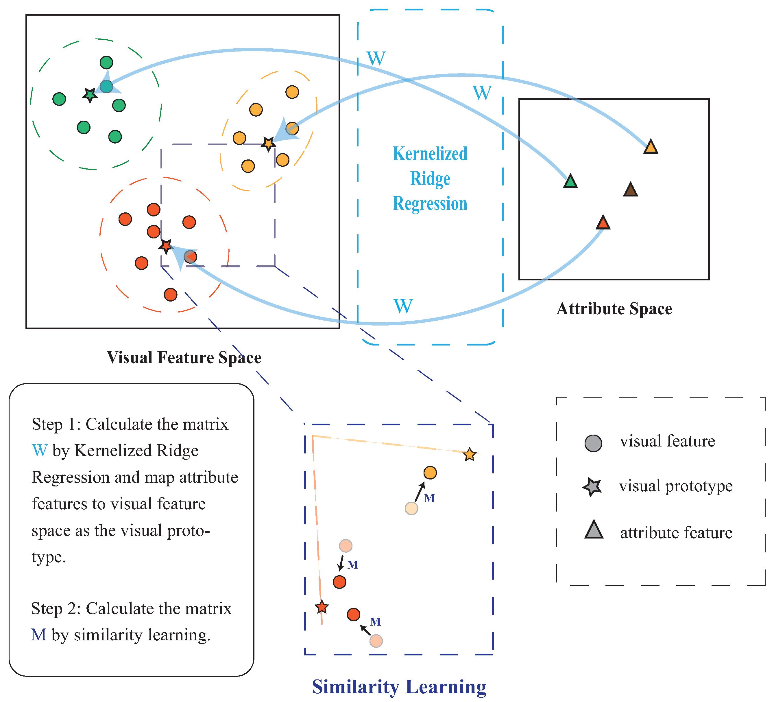
The structure of the proposed method is shown in Figure 1. Our method focuses on kernelized visual prototype learning and kernelized similarity learning for zero-shot recognition. In this section, we explain the proposed method in two steps.
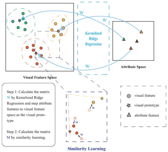
Figure 1.
The structure of the proposed method (W is the projection matrix from the attribute space to the visual feature space, and M is the transformer matrix that brings data points closer to the corresponding prototype).
Let denote the set of instances from seen classes, where is the -dimensional visual feature vector for the instance. Let and represent the sets of seen and unseen class labels, respectively, where and denote the set of all labels. Moreover, each class label corresponds to , where is the -dimensional semantic feature vector of the class c. The class label of is denoted by . The ZSL classification task can be described as , where the model predicts . In addition, in GZSL classification, new instances are from all classes (both seen and unseen).
Let be the visual prototype of class c. Define the kernelized similarity function for calculating the similarity of each instance to all visual prototypes . The kernel function uplifts the visual feature vector to a higher-dimensional space to achieve nonlinearization, and the similarity is calculated as shown in Equation (9).
where W is a projection matrix and k is a selected kernel function. Kernelized similarity involves replacing the common vector inner product with a kernel to create the nonlinear mapping part.
The set of prototypes is derived and utilized to learn the similarity function. In the first subsection, with some theoretical proof, the method for obtaining suitable is presented. Then, we introduce the kernelized similarity function and the kernel polarization methods in the second subsection.
4.1. Prototype Learning
In learning kernelized similarity, the corresponding prototype of the visible class must first be given. Therefore, the proposed method requires prototype learning as the first step. Two different approaches to learning prototypes were mentioned earlier, one for late learning [24] and one for early learning [23]. The former sets the initial prototype as the average of instances from the same visible class, then assumes a mapping function with parameters to map semantic features to prototypes, minimizes the error of the mapped semantic features to the prototypes by adjusting the parameters, and uses the learned function to map semantic feature vectors to the visual prototype. In the latter case, the parameters are adjusted so that the semantic features are mapped to prototypes that are as similar as possible to instances from the same seen classes in order to facilitate the classification task. In early learning, prototypes are generated directly by the mapping function rather than by the mean of the associated instances. It is proved below that when the mapping function is linear, the weight matrices obtained from early and late learning are similar to the objective function formed by the mean square error. In early learning, the general objective function is given by Equation (10):
Furthermore, the objective function is rewritten as a matrix formula in Equation (11):
where X and A are the matrices whose columns are and , respectively.
To find the matrix W that minimizes , first find the partial derivative function of with respect to W, and then set the partial derivative equal to 0 to solve for W:
On the one hand, let and let be the one-hot code matrix from the seen class associated with such that . Let , where is the average of the instances belonging to the same seen class. It is claimed that after replacing all corresponding elements from X with elements from (of the same seen classes), that is, replacing each class instance with the mean of the class, the result of the summation by class remains unchanged. This assertion can be expressed by the following Equation (13):
where the matrix is the transformed matrix obtained after replacing with the mean of the same classes. Thus, Equation (14) can be derived from Equations (12) and (13):
At this point, it is not possible to multiply the inverse of directly on both sides of Equation (15) because it is not known whether it exists.
On the other hand, in late learning, let , and replace in Equation (11) with . Hence, is rewritten, as shown in Equation (16):
Similar to the solution in early learning, the that minimizes J can be found, with the result given in Equation (17):
Since the columns of H are one-hot vectors, the columns of the matrix H are linearly independent, which makes invertible. Hence,
After finding , the optimization method minimizes the Frobenius norm in order to obtain the best projection matrix from A to . The following Equation (19) is obtained by setting the derivative to zero:
When comparing Equation (15) with Equation (19), the form of in Equation (15) is similar to that of W in Equation (19). If the columns of the matrix A are linearly independent such that is invertible, W can be uniquely represented as . Thus, when using linear mapping functions, early learning with the objective of minimizing the mean square error produces parameters similar to those of late learning. To reduce the number of calculations, late learning is chosen, where the means of the instances from the corresponding seen classes are considered the true prototypes.
Since the dataset used for testing has an imbalance in the number of instances per class, directly ignoring this imbalance using the Frobenius norm minimization method may not effectively reduce the impact of data imbalance. Ridge regression improves generalization by preventing the weights from being biased toward a class with a large number of instances. The kernel function is used to enhance the nonlinear component and relate the semantic features of the seen classes to those of the unseen classes. Therefore, a kernelized ridge regression method is used instead of the original form, which avoids the effects of using linear mapping. The common form of ridge regression is given in Equation (20):
where is a non-negative regularization hyperparameter.
Similar to the previous solution, the optimal is solved by first finding the derivative function of J with respect to and then setting the derivative function to zero, as shown in Equation (21).
with the above form, the variable is defined by Equation (22) to reformulate Equations (21)–(23).
To simplify the form of Equation (21), the variable is introduced, which is defined as shown in Equation (22). By introducing the variable into Equation (21), Equation (21) can be simplified to the form of Equation (23):
Then, using Equation (23) in Equation (22), Equation (22) can be rewritten as Equation (24):
which implies that
A kernel matrix can be computed for the semantic vectors of the seen classes as a pairwise similarity of the class vectors using a kernel function k, and Equation (25) can be reformulated as Equation (26):
Finally, let represent the visual prototype of the unseen class , which can be computed by Equation (27):
where each element of is the inner product of the semantic feature vectors of the unseen classes and the semantic feature vectors of each seen class computed by the kernel function. Furthermore, is the coordinate in the space generated by the base consisting of the column vectors in .
4.2. Similarity Learning
In ZSL, maximum similarity is often used to discriminate between the correct unseen class labels, which commonly takes the form of the inner product of vectors. Considering the maximization of intraclass similarity, this paper follows another approach with the autoencoder structure. The similarity function is presented in Equation (28):
where M is the learned weight matrix. Proposition 1 implies that the goal of maximizing Equation (28) is to find an orthogonal matrix solution, , for which its column vectors are weakly incoherent. Therefore, the weight matrix M is constrained in an implicit manner. Such a constrained M creates greater similarity between the data points and corresponding prototypes than an unconstrained M.
Although the above formula contains the autoencoder structure, the weakness of this similarity function is that it is merely a linear mapping between the old and the new . Thus, kernel methods are used to reformulate the similarity function in this paper. Let denote the RBF kernels, and the similarity function is then rewritten as Equation (29):
Due to the kernels, Equation (29) contains a nonlinear component. However, the similarity function defined in this way only considers maximizing intraclass similarity, and, for better classification, interclass similarity must also be reduced. Therefore, in the following, kernel polarization is applied in Equation (29).
Let denote the set of corresponding class labels, one for each data point. Following Proposition 3, the objective function is given by Equation (30):
where is formed as Equation (31). is the class label corresponding to , and denotes the prototype corresponding to class . equals one when and when , equals zero. preserves the similarity of instances within the same class. In contrast, for instances that are not from the same class, contributes to the non-diagonal entries of the matrix , which reduces the similarity between instances from different classes.
Moreover, this term moves within-class samples closer to each other. In contrast, contributes to the off-diagonal entries of L and moves between-class samples away from each other. Thus, controls a form of regularization, which balances positive and negative entries.
The final goal of similarity learning is to find the best projection matrix M that maximizes the objective function, as given by Equation (30). Fix and , and let . Our approach is demonstrated in detail as follows.
Then, we give the objective function concerning M that needs to be optimized:
where denotes the set of all seen class labels, except for , and denotes the prototype corresponding to class j. In order for the algorithm to converge slightly faster, we set and instead of and , respectively. Also, we set for simplicity.
Then, the corresponding gradient is computed for the gradient descent method, and the weight matrix is updated using Equation (35) as follows:
where is the set of indices of size I in the t-th batch and is the learning rate. As the algorithm is applied within different domains (instances from the same class), the learning rate should be adjusted accordingly. Root Mean Square Propagation (RMSprop) [30] is a more appropriate method, where calculates the weighted moving average of the squared gradient, with being the decaying rate:
Furthermore, if the kernel function does not impose soft/implicit incoherence on M, Equation (34) can be simplified to Equation (37):
The proposed method consists of two parts, the first part is prototype learning, which simply involves computing the prototype according to Equations (26) and (27). The pseudo-code of the algorithm in the second part is shown in Algorithm 1.
| Algorithm 1 Optimization of the objective function |
|
4.3. Classification
In prototype learning, we gain a new prototype of each unseen class. Having learned , we calculate the similarity between the instance to be classified and all visual prototypes , based on the weight matrix and kernel function, and take the class with the highest similarity as the classification result during testing:
where k is the same kernel function as in training and is determined using Equation (27). Since the proposed method is required to compute the vector dot product, for this kind of nearest neighbor classification, a useful method is the kernel approximation approach (e.g., Nystrom approximation [31]). However, this is beyond the scope of our research, and we will explore the effectiveness of this approximation in an algorithm in future work.
5. Experiments and Evaluation
Since the classification space of the algorithm is a visual feature space, and images cannot be used directly for classification, the image features first need to be extracted as feature vectors. For visual feature vectors, we extracted 2048-dimensional feature vectors from the images using ResNet-152 [32], pooled as top-level average pooling, and pre-trained on the ImageNet dataset [33]. For semantic feature vectors, we used attribute feature vectors (real-value type) for each class in the dataset.
The proposed method was evaluated on five ZSL datasets: Attribute Pascal and Yahoo (aPY) [2], Animals with Attributes (AWA1) [34], Animals with Attributes 2 (AWA2) [33], Caltech-UCSD Birds (CUB) [34], and SUN Attributes (SUN) [35]. The detailed elements of the utilized datasets are presented in Table 2. The data-splitting method used in the experiments is detailed in Table 3, and, since the visual features were pre-trained on ImageNet, we needed to ensure that there were no common classes between the datasets involved in the testing and ImageNet. We processed visual and semantic feature vectors using two basic data preprocessing methods: mean subtraction and -norm normalization.
Table 2.
Description of the basic elements of the datasets.
Table 3.
Dataset split used in experiments. (S represents seen classes, and U represents unseen classes).
Table 4 shows all the kernel functions and their derivatives used in the experiments. The first step of the proposed method is kernelized ridge regression, in which the kernel function we chose was the Gaussian kernel and for all -normalized datasets. The parameter in the kernel function and the hyperparameter of kernelized ridge regression were determined using cross-validation. The second step of the proposed method is similarity learning, and the parameters in the algorithm were set as follows: , , the parameter was set to for the RMSprop solver [30], and the datasets were trained using SGD for 5-12 epochs.
Table 4.
Derivatives of various kernel functions with respect to M.
To evaluate the proposed ZSL method, we report the average top-1 accuracy per class for classification tasks performed on unseen classes, which is calculated as shown in Equation (39):
where is the number of unseen classes. For the GZSL protocol, both seen and unseen classes are involved in the testing phase, and let denote the average per-class top-1 accuracy of the seen class, calculated in the same way as . Then, we use the harmonic mean [33] to evaluate the performance of our method for GZSL, which is calculated as shown in Equation (40):
This strategy can identify when the proposed method overfits to either seen or unseen classes for both ZSL and GZSL.
5.1. Comparison with Baselines
To evaluate the effectiveness, the proposed zero-shot kernel learning approach was compared with several methods, including DAP and IAP [34], CONSE [36], CMT [37], SSE [38], LATEM [39], ALE [7], DEVISE [6], SJE [40], ESZSL [41], SYNC [42], SAE [11], PLNPS [3], APN [43], and CCZSL [44].
5.1.1. Zero-Shot Learning
Table 5 demonstrates the ZSL classification accuracy of the proposed method with respect to different kernel functions. It can be observed that the Gaussian-Ort kernel achieved the best performance, followed by the Cauchy-Ort kernel. The methods with implicit incoherence constraints on M outperformed the unconstrained methods on all five datasets, and the unconstrained methods also performed worse than the Linear kernel. The performance of the proposed method on the CUB dataset did not significantly improve.
Table 5.
Accuracy(%) on the unseen classes for all compared methods. (Average Rank) column indicates the average rank of the accuracy on five benchmark datasets. The best results are shown in bold, and the second-best results are underlined. Missing results are indicated with a −.
It is hypothesized that the superior performance of the Gaussian kernel can be attributed to its ability to map data points to a hidden infinite-dimensional Hilbert space, where decision boundaries can be easily identified and data points can be classified according to the assigned labels. Also, the orthogonality of the kernel ensures that the constructed mappings are autoencoder-like, which guarantees the correct distribution of the semantic features when mapped to the visual feature space, mitigating certain DSPs.
5.1.2. Generalized Zero-Shot Learning
Table 6 presents the results of our experiments and the scores obtained for GZSL. When comparing the generalized score (H), the proposed method with the Cauchy-Ort kernel outperformed other methods on the AWA1 and aPY datasets (2/5). The generalized score (H) is a composite indicator of the model’s classification performance in all classes. In terms of this score, the Cauchy-Ort kernel was closely followed by the Gaussian-Ort kernel and outperformed the other methods on the SUN dataset (1/5). In particular, on the aPY dataset, the Cauchy-Ort and Gaussian-Ort kernels obtained the best and second-best accuracies, respectively, which implies that the Cauchy-Ort kernel outperformed the Gaussian-Ort kernel. Similar to the ZSL results, the performance of the proposed method on the CUB dataset did not significantly improve.
Table 6.
GZSL evaluations on aPY, CUB, SUN, AWA1, and AWA2. = average per-class accuracy of unseen classes, = average per-class accuracy of seen classes, and H = harmonic mean. The best results are shown in bold, and the second-best results are underlined. Missing results are indicated with a −.
It should be noted that the models that imposed implicit incoherence continued to demonstrate superior performance compared to the variants that did not impose it. Furthermore, the Cauchy kernel was observed to be a suitable option for a range of testing tasks. The Cauchy kernel may be less susceptible to overfitting to local clusters of data points, as its tails decay more gradually in comparison to the tails of a Gaussian kernel.
5.2. Sensitivity Analysis
In this section, we show how the proposed method behaved with respect to the choice of the radius of the Gaussian and Cauchy kernels, the bias c of the linear kernel, and the regularization parameter in Equation (32) to analyze robustness. The robust algorithm avoided overfitting and exhibited better generalization ability, while the sensitivity of hyperparameter selection was studied for better fine-tuning.
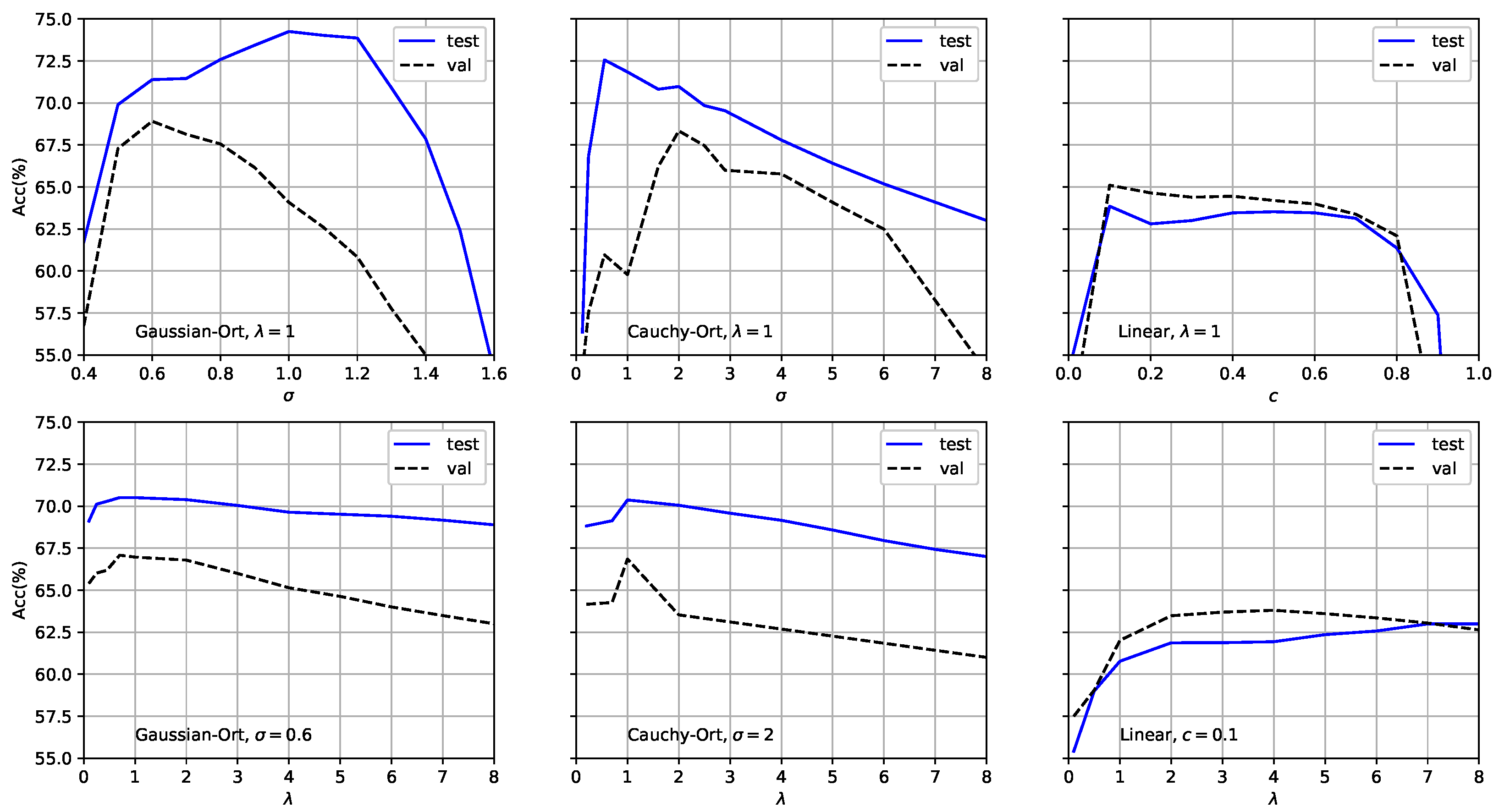
Figure 2 shows the ZSL classification accuracy of the proposed method on the AWA2 dataset with respect to the above hyperparameters. The plot shows that the radius is an important hyperparameter in the proposed method. For the Gaussian-Ort kernel, the validation and test curves were relatively smooth. The best results were obtained at = 0.6 and = 1, respectively, and the testing accuracy was consistently higher than the validation accuracy. A similar trend was observed for the Cauchy-Ort kernel. The difference between the testing and validation accuracies indicated a domain-shift problem, which is common in knowledge transfer tasks. For the Linear kernel, the testing and validation accuracies were not significantly different and reached a maximum at , but were lower than those of the Gaussian-Ort and Cauchy-Ort kernels. This demonstrates that while the Linear kernel generalized well, it lacked the ability to represent nonlinear data patterns.
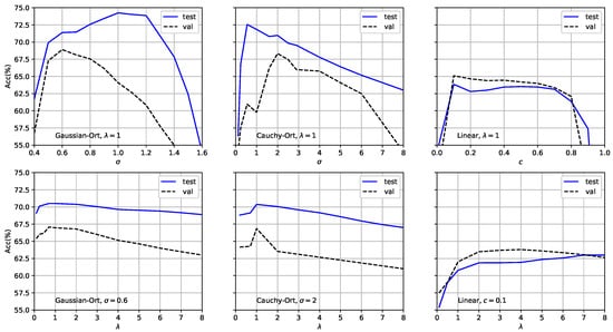
Figure 2.
ZSL accuracy on the AWA2 dataset for the validation and test sets. We varied , , and c. In the top row, we fixed and varied and c for the kernel functions. The bottom row shows the performance of the proposed method with respect to regularized while fixing either or c, previously chosen through cross-validation.
Figure 2 (bottom) shows the accuracy with respect to the regularization parameter , which controls the extent to which data points projected onto the same space are pushed against each other. For all kernel functions in the experiment, the values of corresponding to the peaks in the testing and validation accuracies were almost identical. The value of had little effect on the performance of the proposed method, and the interval to reach the best performance was (0.8, 2). However, it is clear that as or , the classification performance of the proposed method significantly degrades. This indicates the importance of balancing the effects of intra- and interclass statistics due to kernel polarization.
5.3. Visual Prototype Learning
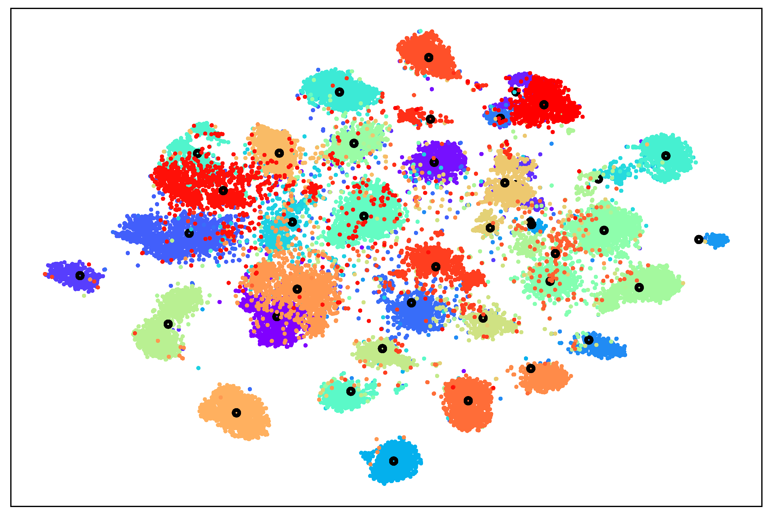
This method classifies semantic features by first obtaining their prototypes in the visual feature space and then considering the distance from the instances to the step-by-step prototypes without affecting each other. Therefore, it is important to choose a suitable and distinguishable visual prototype. Figure 3 shows the visualization results of the visible class instances and means on the AWA2 dataset using t-SNE. Due to the use of similarity for classification, although some class instances were at the fuzzy boundary of classification, the prototypes (means) of each class maintained a suitable distance from each other and were distinguishable, so it was appropriate to use the mean of the visual feature as the prototype.
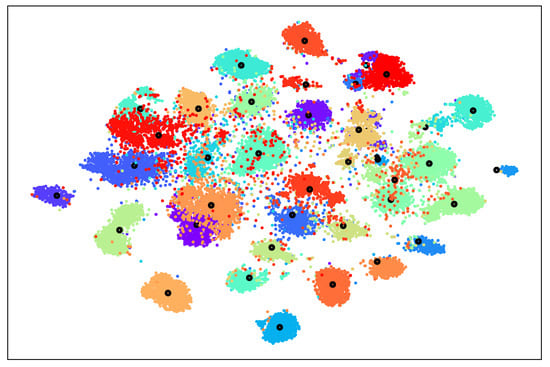
Figure 3.
Distribution of seen classes in the AWA2 dataset using t-SNE visualization. Black circles indicate visual prototypes (class averages).
5.4. Kernel Effect on Visual Prototype Learning
Since the prototypes of the unseen classes were obtained through kernelized ridge regression, we needed to evaluate the effect of using different kernels on the final performance of kernelized ridge regression. This subsection uses a simple model: kernelized ridge regression + Euclidean distance nearest neighbor search. The accuracy was calculated on the AWA2 dataset using three different kernel functions: Linear, Gaussian, and Cauchy. In Figure 4, the results show that the Gaussian kernel achieved the highest accuracy of 70.5%, followed by the Cauchy kernel with an accuracy of 70.4%, and it can be seen that the difference between the two was very small (0.1%). For the Linear kernel, the difference in accuracy did not reach 5%. It can be seen that the selection of the prototype learning kernel is not as important as the selection of the similarity learning kernel, considering the impact of different kernels on model performance.
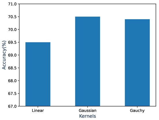
Figure 4.
Classification accuracy of the simple model on the AWA2 dataset using different kernel functions.
6. Conclusions
First, we constructed a visual prototype of the unseen class through kernelized ridge regression and then used kernel polarization and an autoencoder structure to construct a similarity function for calculating the similarity from the unseen class instances to the visual prototypes, which was then applied to ZSL and GZSL recognition tasks. Moreover, a novel approach based on kernelized similarity learning was proposed, aiming to adjust the similarity between visual instances and all prototypes. To evaluate the classification performance of our method, experiments were performed on five ZSL benchmark datasets. The proposed method demonstrated superior performance compared to SOTA methods in the majority of cases under both ZSL and GZSL settings. Further investigations into the impact of noise on the proposed approach and enhancements to the computational efficiency of the kernelized inner product may be warranted in the future.
Author Contributions
K.C. wrote the main manuscript, proposed the methodology, designed the experiments, programmed, and prepared the figures and tables. B.F. proposed the ideas, validated the results, and reviewed the manuscript. All authors have read and agreed to the published version of the manuscript.
Funding
This research was funded by National Natural Science Foundation of China grant number 12001412.
Data Availability Statement
The authors confirm that the data supporting the findings of this study are openly available at AwA: https://cvml.ista.ac.at/AwA/, accessed on 5 August 2024; AwA2: https://cvml.ista.ac.at/AwA2/, accessed on 5 August 2024; SUN: https://vision.princeton.edu/projects/2010/SUN/, accessed on 5 August 2024; CUB: https://www.vision.caltech.edu/datasets/cub_200_2011/, accessed on 5 August 2024; and aPY: https://vision.cs.uiuc.edu/attributes/, accessed on 5 August 2024.
Conflicts of Interest
No potential conflicts of interest were reported by the authors.
References
- Lampert, C.H.; Nickisch, H.; Harmeling, S. Learning to detect unseen object classes by between-class attribute transfer. In Proceedings of the 2009 IEEE Conference on Computer Vision and Pattern Recognition, Miami, FL, USA, 20–25 June 2009; pp. 951–958. [Google Scholar] [CrossRef]
- Farhadi, A.; Endres, I.; Hoiem, D.; Forsyth, D. Describing objects by their attributes. In Proceedings of the 2009 IEEE Conference on Computer Vision and Pattern Recognition, Miami, FL, USA, 20–25 June 2009; pp. 1778–1785. [Google Scholar] [CrossRef]
- Zhang, H.; Mao, H.; Long, Y.; Yang, W.; Shao, L. A probabilistic zero-shot learning method via latent nonnegative prototype synthesis of unseen classes. IEEE Trans. Neural Netw. Learn. Syst. 2019, 31, 2361–2375. [Google Scholar] [CrossRef] [PubMed]
- Jiang, H.; Wang, R.; Shan, S.; Chen, X. Adaptive metric Learning for Zero-Shot recognition. IEEE Signal Process. Lett. 2019, 26, 1270–1274. [Google Scholar] [CrossRef]
- Bhagat, P.; Choudhary, P.; Singh, K.M. A study on zero-shot learning from semantic viewpoint. Vis. Comput. 2023, 39, 2149–2163. [Google Scholar] [CrossRef]
- Frome, A.; Corrado, G.S.; Shlens, J.; Bengio, S.; Dean, J.; Ranzato, M.; Mikolov, T. A deep visual-semantic embedding model. Neural Inf. Process. Syst. 2013, 26, 2121–2129. [Google Scholar]
- Akata, Z.; Perronnin, F.; Harchaoui, Z.; Schmid, C. Label-embedding for image classification. IEEE Trans. Pattern Anal. Mach. Intell. 2016, 38, 1425–1438. [Google Scholar] [CrossRef] [PubMed]
- Ji, Z.; Yu, Y.; Pang, Y.; Guo, J.; Zhang, Z. Manifold regularized cross-modal embedding for zero-shot learning. Inf. Sci. 2017, 378, 48–58. [Google Scholar] [CrossRef]
- Ma, P.; Hu, X. A variational autoencoder with deep embedding model for generalized zero-shot learning. In Proceedings of the AAAI Conference on Artificial Intelligence, New York, NY, USA, 7–12 February 2020; Volume 34, pp. 11733–11740. [Google Scholar] [CrossRef]
- Pan, C.; Huang, J.; Jiang, H.; Gong, J. Towards zero-shot learning generalization via a cosine distance loss. Neurocomputing 2020, 381, 167–176. [Google Scholar] [CrossRef]
- Kodirov, E.; Xiang, T.; Gong, S. Semantic autoencoder for zero-shot learning. In Proceedings of the IEEE Conference on Computer Vision and Pattern Recognition, Honolulu, HI, USA, 21–26 July 2017; pp. 3174–3183. [Google Scholar]
- Qiao, R.; Liu, L.; Shen, C.; Van Den Hengel, A. Visually aligned word embeddings for improving zero-shot learning. arXiv 2017, arXiv:1707.05427. [Google Scholar] [CrossRef]
- Liu, H.; Yao, L.; Zheng, Q.; Luo, M.; Zhao, H.; Lyu, Y. Dual-stream generative adversarial networks for distributionally robust zero-shot learning. Inf. Sci. 2020, 519, 407–422. [Google Scholar] [CrossRef]
- Liu, J.; Zhang, Z.; Yang, G. Cross-class generative network for zero-shot learning. Inf. Sci. 2021, 555, 147–163. [Google Scholar] [CrossRef]
- Xian, Y.; Lorenz, T.; Schiele, B.; Akata, Z. Feature generating networks for zero-shot learning. arXiv 2017, arXiv:1712.00981. [Google Scholar] [CrossRef]
- Felix, R.; Kumar, B.G.V.; Reid, I.; Carneiro, G. Multi-modal cycle-consistent generalized zero-shot learning. In Proceedings of the European Conference on Computer Vision (ECCV), Munich, Germany, 8–14 September 2018; pp. 21–37. [Google Scholar]
- Li, J.; Jin, M.; Lü, K.; Ding, Z.; Zhu, L.; Huang, Z.X. Leveraging the invariant side of generative zero-shot learning. arXiv 2019, arXiv:1904.04092. [Google Scholar] [CrossRef]
- Fang, J.; Yang, G.; Han, A.; Liu, X.; Chen, B.; Wang, C. Zero-shot learning via categorization-relevant disentanglement and discriminative samples synthesis. Vis. Comput. 2024, 40, 3889–3901. [Google Scholar] [CrossRef]
- Fu, Y.; Hospedales, T.M.; Xiang, T.; Gong, S. Transductive multi-view zero-shot learning. IEEE Trans. Pattern Anal. Mach. Intell. 2015, 37, 2332–2345. [Google Scholar] [CrossRef] [PubMed]
- Shigeto, Y.; Suzuki, I.; Hara, K.; Shimbo, M.; Matsumoto, Y. Ridge regression, hubness, and zero-shot learning. In Proceedings of the Machine Learning and Knowledge Discovery in Databases: European Conference (ECML PKDD 2015), Porto, Portugal, 7–11 September 2015; Proceedings, Part I 15. Springer International Publishing: Cham, Switzerland, 2015; pp. 135–151. [Google Scholar]
- Ji, Z.; Wang, J.; Yu, Y.; Pang, Y.; Han, J. Class-specific synthesized dictionary model for Zero-Shot Learning. Neurocomputing 2019, 329, 339–347. [Google Scholar] [CrossRef]
- Bucher, M.; Herbin, S.; Jurie, F. Improving semantic embedding consistency by metric learning for Zero-Shot classiffication. In Proceedings of the Computer Vision–ECCV 2016: 14th European Conference, Amsterdam, The Netherlands, 11–14 October 2016; Proceedings, Part V 14. Springer International Publishing: Cham, Switzerland, 2016; pp. 730–746. [Google Scholar]
- Zhang, L.; Xiang, T.; Gong, S. Learning a deep embedding model for zero-shot learning. In Proceedings of the IEEE Conference on Computer Vision and Pattern Recognition, Honolulu, HI, USA, 21–26 July 2017; pp. 2021–2030. [Google Scholar]
- Changpinyo, S.; Chao, W.; Sha, F. Predicting visual exemplars of unseen classes for zero-shot learning. In Proceedings of the IEEE International Conference on Computer Vision, Venice, Italy, 22–29 October 2017; pp. 3476–3485. [Google Scholar]
- Mensink, T.; Verbeek, J.; Perronnin, F.; Csurka, G. Distance-based image classification: Generalizing to new classes at near-zero cost. IEEE Trans. Pattern Anal. Mach. Intell. 2013, 35, 2624–2637. [Google Scholar] [CrossRef]
- Verma, V.K.; Rai, P. A simple exponential family framework for zero-shot learning. In Proceedings of the Machine Learning and Knowledge Discovery in Databases: European Conference, Skopje, Macedonia, 18–22 September 2017; Springer: Berlin/Heidelberg, Germany, 2017; pp. 792–808. [Google Scholar]
- Zhang, H.; Koniusz, P. Zero-shot kernel learning. In Proceedings of the 2018 IEEE/CVF Conference on Computer Vision and Pattern Recognition, Salt Lake City, UT, USA, 18–23 June 2018; pp. 7670–7679. [Google Scholar] [CrossRef]
- Baram, Y. Learning by kernel polarization. Neural Comput. 2005, 17, 1264–1275. [Google Scholar] [CrossRef]
- Minh, H.Q.; Niyogi, P.; Yao, Y. Mercer’s theorem, feature Maps, and smoothing. In Proceedings of the International Conference on Computational Learning Theory, Pittsburgh, PA, USA, 22–25 June 2006; pp. 154–168. [Google Scholar] [CrossRef]
- Peng, Y.L.; Lee, W.P. Practical guidelines for resolving the loss divergence caused by the root-mean-squared propagation optimizer. Appl. Soft Comput. 2024, 153, 111335. [Google Scholar] [CrossRef]
- Abedsoltan, A.; Pandit, P.; Rademacher, L.; Belkin, M. On the Nyström approximation for preconditioning in kernel machines. In Proceedings of the 27th International Conference on Artificial Intelligence and Statistics, Valencia, Spain, 2–4 May 2024; pp. 3718–3726. [Google Scholar]
- He, K.; Zhang, X.; Ren, S.; Sun, J. Deep residual learning for image recognition. In Proceedings of the IEEE Conference on Computer Vision and Pattern Recognition, Las Vegas, NV, USA, 27–30 June 2016; pp. 770–778. [Google Scholar]
- Xian, Y.; Lampert, C.H.; Schiele, B.; Akata, Z. Zero-shot learning: A comprehensive evaluation of the good, the bad and the ugly. IEEE Trans. Pattern Anal. Mach. Intell. 2019, 41, 2251–2265. [Google Scholar] [CrossRef]
- Lampert, C.H.; Nickisch, H.; Harmeling, S. Attribute-based classification for zero-shot visual object categorization. IEEE Trans. Pattern Anal. Mach. Intell. 2014, 36, 453–465. [Google Scholar] [CrossRef]
- Patterson, G.; Hays, J. SUN attribute database: Discovering, annotating, and recognizing scene attributes. In Proceedings of the 2012 IEEE Conference on Computer Vision and Pattern Recognition, Providence, RI, USA, 16–21 June 2012; pp. 2751–2758. [Google Scholar] [CrossRef]
- Norouzi, M.; Mikolov, T.; Bengio, S.; Singer, Y.; Shlens, J.; Frome, A.; Corrado, G.S.; Dean, J. Zero-shot learning by convex combination of semantic embeddings. arXiv 2013, arXiv:1312.5650. [Google Scholar]
- Socher, R.; Ganjoo, M.; Manning, C.D.; Ng, A. Zero-shot learning through cross-Modal transfer. In Proceedings of the Advances in Neural Information Processing Systems, Lake Tahoe, NV, USA, 5–8 December 2013; pp. 934–943. [Google Scholar]
- Zhang, Z.; Saligrama, V. Zero-shot learning via semantic similarity embedding. In Proceedings of the IEEE International Conference on Computer Vision, Santiago, Chile, 7–13 December 2015; pp. 4166–4174. [Google Scholar]
- Xian, Y.; Akata, Z.; Sharma, G.; Nguyen, Q.; Hein, M.; Schiele, B. Latent embeddings for zero-shot classification. In Proceedings of the IEEE Conference on Computer Vision and Pattern Recognition, Las Vegas, NV, USA, 27–30 June 2016; pp. 66–77. [Google Scholar]
- Akata, Z.; Reed, S.; Walter, D.; Lee, H.; Schiele, B. Evaluation of output embeddings for fine-grained image classification. In Proceedings of the IEEE Conference on Computer Vision and Pattern Recognition, Boston, MA, USA, 7–12 June 2015; pp. 2927–2936. [Google Scholar]
- Romera-Paredes, B.; Torr, P. An embarrassingly simple approach to zero-shot learning. In Proceedings of the 32nd International Conference on Machine Learning, Lille, France, 6–11 July 2015; pp. 2152–2161. [Google Scholar]
- Changpinyo, S.; Chao, W.L.; Gong, B.; Sha, F. Synthesized classifiers for zero-shot learning. In Proceedings of the IEEE Conference on Computer Vision and Pattern Recognition, Las Vegas, NV, USA, 27–30 June 2016; pp. 5327–5336. [Google Scholar]
- Xu, W.; Xian, Y.; Wang, J.; Schiele, B.; Akata, Z. Attribute Prototype Network for Zero-Shot Learning. In Proceedings of the Advances in Neural Information Processing Systems, Online, 6–12 December 2020; pp. 21969–21980. [Google Scholar]
- Cheng, D.; Wang, G.; Wang, N.; Zhang, D.; Zhang, Q.; Gao, X. Discriminative and robust attribute alignment for zero-shot learning. IEEE Trans. Circuits Syst. Video Technol. 2023, 33, 4244–4256. [Google Scholar] [CrossRef]

Disclaimer/Publisher’s Note: The statements, opinions and data contained in all publications are solely those of the individual author(s) and contributor(s) and not of MDPI and/or the editor(s). MDPI and/or the editor(s) disclaim responsibility for any injury to people or property resulting from any ideas, methods, instructions or products referred to in the content. |
© 2025 by the authors. Licensee MDPI, Basel, Switzerland. This article is an open access article distributed under the terms and conditions of the Creative Commons Attribution (CC BY) license (https://creativecommons.org/licenses/by/4.0/).