On the Inversion of the Mellin Convolution

Abstract

The deconvolution of the Mellin convolution is studied for a great variety of functions that are expressed in terms of $\alpha$–log-exponential monomials. It is shown that the generation of pairs of functions satisfying a Sonin-like condition can be worked as a deconvolution process. Applications of deconvolution to scale-invariant linear systems are presented.

1. Introduction

As the Duhamel convolution plays a very important role in modulating and describing linear shift-invariant systems [1,2,3,4], the Mellin convolution plays the same role in scale-invariant systems [5,6,7,8,9,10,11]. This has a deep connection with several applications in physics and engineering for dealing with multi-scale wavelet analyses and self-similarity problems [12,13,14,15,16,17].

While the Laplace transform plays an important role in studying shift-invariant systems, the same role is performed by the Mellin transform. Its history is connected to that of the gamma function

$$\Gamma \left(\nu \right)={\int }_0^{\infty }{e}^{-t}{t}^{\nu -1}dt,$$

and its relation with the exponential function

$$e^{-\tau }={\displaystyle \frac{1}{2\pi i}}{\int }_{\gamma }\Gamma \left(t\right){\tau }^{-t}dt,$$

where $\gamma$ is a vertical straight line in the complex plane. The first formula is due to Euler and the second one Pincherle; see [18]. Riemann was the first to apply the Mellin transform to the zeta function problem, but it was Mellin who began to apply a special treatment of this transform that usually is defined by [9,18,19]

$$G\left(\nu \right)=\mathcal{M}\left[g\left(\tau \right)\right]={\int }_0^{\infty }g\left(t\right)t^{\nu -1}dt,$$

(1)

and provided conditions of existence. The number of applications in science and engineering has been increasing in recent times, for example, in economics [20], electromagnetism [21], physics [22], signal processing [23], etc. Currently, one of the main challenges is to extend the Mellin transform theory to the fractional system applications [9,24,25,26].

The Mellin convolution (MC) results from the Mellin transform product defined by

$$x\left(\tau \right)\star g\left(\tau \right)={\int }_0^{\infty }x\left({\displaystyle \frac{\tau }{\eta }}\right)g\left(\eta \right){\displaystyle \frac{d\eta }{\eta }},$$

(2)

and verifying

$$\mathcal{M}\left[x\left(\tau \right)\star g\left(\tau \right)\right]=\mathcal{M}\left[x\left(\tau \right)\right]\mathcal{M}\left[g\left(\tau \right)\right].$$

(3)

Let $g\left(\tau \right),h\left(\tau \right)$, $\tau \in {\mathbb{R}}^{+}$, be two functions and consider their convolution. When there exists a third function $h^{-1}\left(\tau \right)$ such that $\left(g\left(\tau \right)\star h\left(\tau \right)\right)\star h^{-1}\left(\tau \right)=g\left(\tau \right)$, we say that the convolution is invertible and that $h\left(\tau \right)$ and $h^{-1}\left(\tau \right)$ are convolutionally inverse $h^{-1}\left(\tau \right)\star h\left(\tau \right)=\delta (\tau -1)$, where $\delta (.)$ is the Dirac impulse.

These relations constitute the basis for inverting the MC. As we will show, it may happen that this inversion (deconvolution) leads to singular solutions. One of our main objectives is to avoid and solve such problems. To achieve this, we follow quite closely the Abel–Sonin-like procedure [27,28] to express the solutions in terms of linear combinations of $\alpha$–log-exponential functions and other functions resulting from certain modifications of these. To our knowledge, there are no works related to the extension of the Sonin condition to the Mellin convolution case. Another of our main objectives is to systematize the deconvolution process of (2). For this purpose, we rely on an algebraic version of the Mellin convolution [10] and the $\alpha$–log-exponential functions.

Among the referred applications to scale-invariant system deconvolution, we can cite others like [29,30,31,32,33].

This article is structured as follows. Section 2 contains the preliminary results for the development of our work. In Section 3, we deduce the broader Sonin condition from the concept of being convolutionally inverse and solve some examples. We prove that convolutionally inverse implies a broader Sonin condition. In Section 4, we show how we can find convolutionally inverse pairs of different functions. Section 5 contains some applications of our results to scale-invariant linear systems. Finally, the conclusions are presented in Section 6.

2. Properties of Mellin Convolution

Let $g\left(\tau \right)$ be a piecewise continuous function. We redefine the Mellin transform [9] of $g\left(\tau \right)$ as

$$G\left(\nu \right)=\mathcal{M}\left[g\left(\tau \right)\right]={\int }_0^{\infty }g\left(t\right)t^{-\nu -1}dt,$$

(4)

where we make a substitution $\nu \to -\nu$ for establishing better parallelism with the Laplace transform. If $g\left(\tau \right)$ is a function with bounded variation, locally integrable (in the sense that the function is absolutely integrable in any real interval $[a,b]$, so that ${\int }_a^b\left|g\left(\tau \right)\right|d\tau <\infty$, and of polynomial order, then there exists its Mellin transform in a vertical strip in the complex plane (see Remark 1). However, due to the interest in our application, we assume that (4) can be extended into the distributional setup, by assuming that $g\left(\tau \right)$ is a tempered distribution [34], so that we work exclusively with functions having a Mellin transform.

Remark 1.

A function $g\left(\tau \right)$ is of polynomial order if

• For $\tau \to 0^{+}$, there are real constants A, $a>0$, such that $\left|g\left(\tau \right)\right|<A·{\tau }^a$ when τ is small (say, for $\tau <{\tau }_1\in {\mathbb{R}}^{+}$);
• For $\tau \to \infty$, there are real constants B, $b>0$, such that $\left|g\left(\tau \right)\right|<B·{\tau }^b$, when τ is large (say, for $\tau >{\tau }_2\in {\mathbb{R}}^{+}$);
• It holds that $b<a$.

Under these conditions, the integral in (4) converges absolutely and uniformly in a vertical strip in the complex plane defined by $b<\Re \left(\nu \right)<a$, where $G\left(\nu \right)$ is analytic. Therefore, if $g\left(\tau \right)$ and $x\left(\tau \right)$ satisfy the existence conditions of (4), then (2) is well defined and (3) is valid.

We recall the definition of the Mellin convolution (2):

$$x\left(\tau \right)\star g\left(\tau \right)={\int }_0^{\infty }x\left({\displaystyle \frac{\tau }{\eta }}\right)g\left(\eta \right){\displaystyle \frac{d\eta }{\eta }}.$$

We summarize some of the main properties of the Mellin convolution:

• The Mellin convolution is commutative and associative, and its unit element is $\delta (\tau -1)$.

  $$x\left(\tau \right)\star \delta (\tau -1)=x\left(\tau \right).$$
• For $\tau \in {\mathbb{R}}^{+}$ and $\nu \in \mathbb{C}$, it is true that

  $${\tau }^{\nu }\star g\left(\tau \right)=G\left(\nu \right){\tau }^{\nu },$$

  meaning that ${\tau }^{\nu }$ is an eigenfunction of the Mellin convolution with an eigenvalue of the Mellin transform of $g\left(\tau \right)$, $G\left(\nu \right)$).
• For $\alpha \in {\mathbb{R}}^{+}$ [10]

  $${\mathcal{M}}^{-1}\left[v^{-\alpha }\right]\left(\tau \right)={\displaystyle \frac{{ln}^{\alpha -1}\left(\tau \right)}{\Gamma \left(\alpha \right)}}\epsilon (\tau -1),Re\left(v\right)>0.$$

  (5)
  This power function has the following property:

  $${\displaystyle \frac{{ln}^{n\alpha -1}\left(\tau \right)}{\Gamma \left(n\alpha \right)}}\epsilon (\tau -1)\star {\displaystyle \frac{{ln}^{m\alpha -1}\left(\tau \right)}{\Gamma \left(m\alpha \right)}}\epsilon (\tau -1)={\displaystyle \frac{{ln}^{(n+m)\alpha -1}\left(\tau \right)}{\Gamma \left(\right(n+m\left)\alpha \right)}}\epsilon (\tau -1),n,m\in \mathbb{Z}.$$

  (6)
  This property is of great importance because of the structure of $\alpha$–log-exponential monomials.
• The Parseval equality holds true:

  $${\int }_0^{\infty }x\left({\displaystyle \frac{\tau }{\eta }}\right)g\left(\eta \right){\displaystyle \frac{d\eta }{\eta }}={\displaystyle \frac{1}{2\pi j}}{\int }_{\gamma -j\infty }^{\gamma +j\infty }X\left(s\right)G\left(s\right){\tau }^{-s}ds.$$

The Mellin convolution serves to define three types of scale-invariant systems according to the impulse response characteristic (2):

• If $g\left(\tau \right)$ is not identically null for any interval in ${\mathbb{R}}^{+}$, it defines the bilateral systems represented by (2).

  $$y\left(\tau \right)=x\left(\tau \right)\star h\left(\tau \right)={\int }_0^{\infty }x\left({\displaystyle \frac{\tau }{\eta }}\right)g\left(\eta \right){\displaystyle \frac{d\eta }{\eta }}.$$
• The case where $g\left(\tau \right)\equiv 0,\tau <1$ defines the right systems that output the response $y\left(\tau \right)$ is given by

  $$y\left(\tau \right)=x\left(\tau \right)\star h\left(\tau \right)={\int }_1^{\tau }x\left({\displaystyle \frac{\tau }{\eta }}\right)g\left(\eta \right){\displaystyle \frac{d\eta }{\eta }}.$$

  (7)
• When $g\left(\tau \right)\equiv 0,\tau >1,$ the left systems are defined by

  $$y\left(\tau \right)=x\left(\tau \right)\star h\left(\tau \right)={\int }_{\tau }^{1}x\left({\displaystyle \frac{\tau }{\eta }}\right)g\left(\eta \right){\displaystyle \frac{d\eta }{\eta }}.$$

Due to the deep relation with scale systems, we focus on the Hadamard right (left) derivative [9].

Definition 1.

Let $\alpha \in \mathbb{R}$. We define the α-order scale derivative (SD) as the operator ${\mathfrak{D}}_{s_{\pm }}^{\alpha }$ obeying the rule

$${\mathfrak{D}}_{s_{\pm }}^{\alpha }{\tau }^v=v^{\alpha }{\tau }^v,\tau \in {\mathbb{R}}^{+},v\in \mathbb{C},$$

for $Re\left(v\right)>0$ (expansion or stretching case ${\mathfrak{D}}_{s+}^{\alpha }$) or $Re\left(v\right)<0$ (shrinking case ${\mathfrak{D}}_{s-}^{\alpha }$).

The conditions $\Re \left(v\right)>0$ and $\Re \left(v\right)<0$ lead to the cases $\tau \ge 1$ (right) and $0<\tau \le 1$ (left), respectively. The work developed in this article is focused on the case $\tau \ge 1$; the other case is similar. The condition $\tau \ge 1$ leads us to consider right systems (7). Therefore, if $h\left(\tau \right)$ is the impulse response of such a system, then the step response is given by

$$r_{\epsilon }\left(\tau \right)=h\left(\tau \right)\star \epsilon (\tau -1)={\int }_0^{\infty }h\left({\displaystyle \frac{\tau }{\nu }}\right)\epsilon (\nu -1){\displaystyle \frac{d\nu }{\nu }}={\int }_1^{\infty }h\left({\displaystyle \frac{\tau }{\nu }}\right){\displaystyle \frac{d\nu }{\nu }}.$$

Based on the derivative presented in Definition 1, we have the following properties.

• For a function $x\left(\tau \right)$ with a Mellin transform $X\left(v\right)$, it follows that

  $$\mathcal{M}\left[{\mathfrak{D}}_{s+}^{\alpha }x\left(\tau \right)\right]=v^{\alpha }X\left(v\right),$$

  (8)
• $${\mathfrak{D}}_{s_{+}}^{\alpha }\left({\displaystyle \frac{{ln}^{k\alpha -1}\left(\tau \right)}{\Gamma \left(k\alpha \right)}}\epsilon (\tau -1)\right)={\displaystyle \frac{{ln}^{(k-1)\alpha -1}\left(\tau \right)}{\Gamma \left(\right(k-1\left)\alpha \right)}}\epsilon (\tau -1),k\in \mathbb{Z},$$
• $$\begin{array}{cc}\hfill {\mathfrak{D}}_{s_{+}}^{-1}\left({\displaystyle \frac{{ln}^{k\alpha -1}\left(\tau \right)}{\Gamma \left(k\alpha \right)}}\epsilon (\tau -1)\right)& ={\mathcal{M}}^{-1}\left[v^{-(k\alpha +1)}\right]\hfill \\ \hfill & ={\displaystyle \frac{{ln}^{k\alpha }\left(\tau \right)}{\Gamma (k\alpha +1)}}\epsilon (\tau -1).\hfill \end{array}$$

  (9)

These relations suggest us to introduce a very important function for the following developments.

Definition 2.

Let us define the α–log-exponential monomials of order n by

$${\mathcal{E}}_{\gamma ,n}\left(\tau \right)=\sum _{k=n+1}^{\infty }\left({\displaystyle \genfrac{}{}{0pt}{}{k-1}{n}}\right){\gamma }^{k-n-1}{\displaystyle \frac{{ln}^{k\alpha -1}\left(\tau \right)}{\Gamma \left(k\alpha \right)}}\epsilon (\tau -1),\gamma \in \mathbb{C},n\in {\mathbb{N}}_0.$$

(10)

We can show that

$$\mathcal{M}\left[{\mathcal{E}}_{\gamma ,n}\left(\tau \right)\right]={\displaystyle \frac{1}{{\left({\nu }^{\alpha }-\gamma \right)}^{n+1}}},$$

(11)

which is very important in inverting transforms that are expressed as quotients of polynomials.

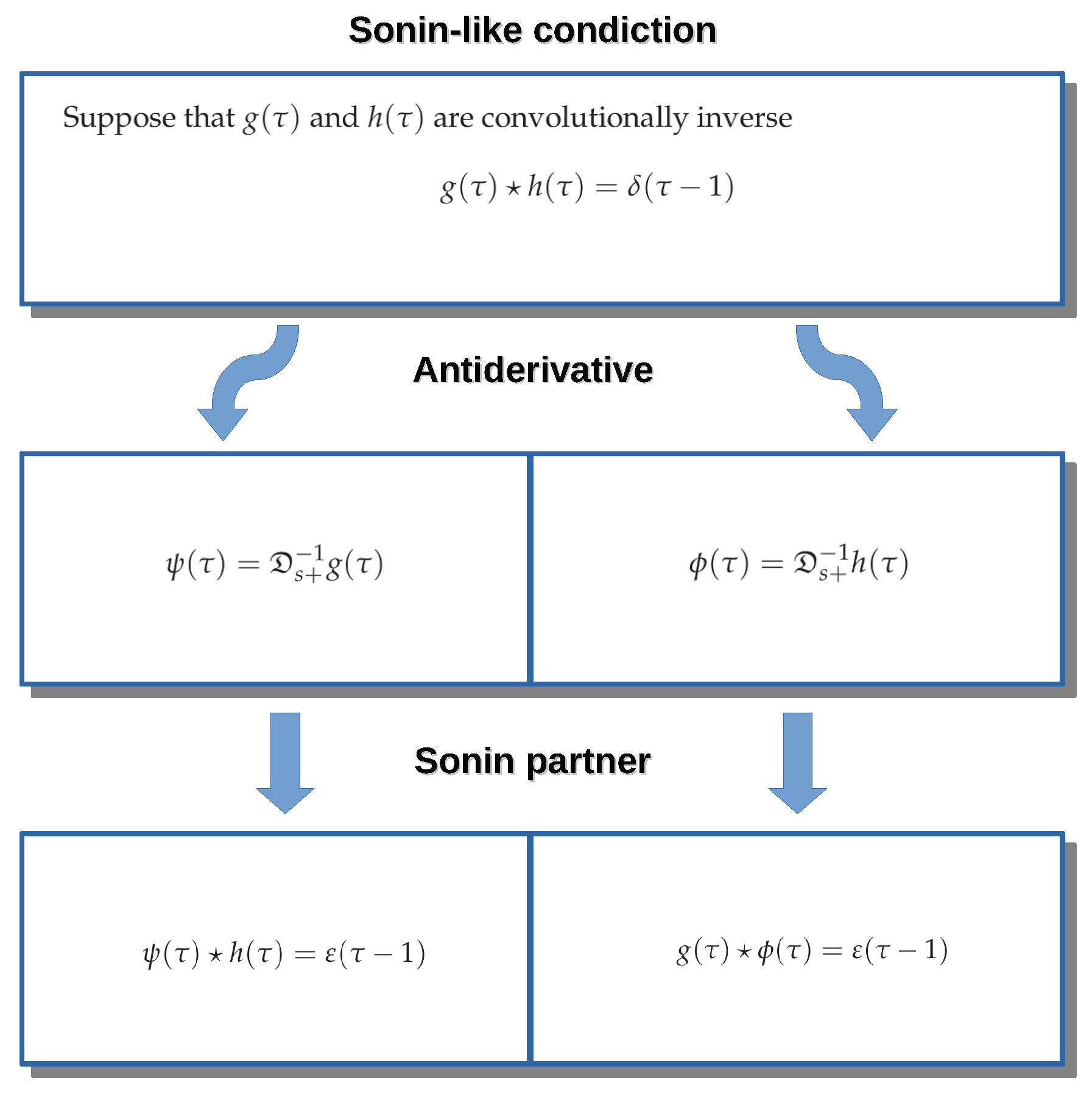
3. Sonin-like Condition

In 1823, Abel presented the generalization of a tautochrone problem [35] whose solution gave rise to one of the first integral equations

$$\varphi \left(t\right)={\int }_0^t{\displaystyle \frac{s^{\prime }\left(t\right)}{{(t-\tau )}^{\alpha }}}d\tau ,t\ge 0,0<\alpha <1,$$

(12)

where $s\left(t\right)$ is the solution. Interestingly, (12) is the usual shift-invariant convolution

$$\varphi \left(t\right)=t^{-\alpha }\ast s^{\prime }\left(t\right).$$

(13)

Abel’s procedure for solving the integral Equation (12) was essentially an algorithm for inverting a linear convolution, suitable for dealing with a singular kernel (impulse response).

In 1884, Sonin published some result related a Abel’s solution [36]. He noted that many of Abel’s results were supported by the formula

$${\displaystyle \frac{t^{\alpha -1}}{\Gamma \left(\alpha \right)}}\ast {\displaystyle \frac{t^{-\alpha }}{\Gamma (-\alpha +1)}}={\displaystyle \frac{d}{dt}}{\displaystyle \frac{t^{\alpha }}{\Gamma (\alpha +1)}}\ast {\displaystyle \frac{t^{-\alpha }}{\Gamma (-\alpha +1)}}=\epsilon \left(t\right).$$

(14)

Sonin verified that Abel, by solving (12), had indeed performed a deconvolution. That is, Abel found a function $\theta \left(t\right)$ such that $\theta \left(t\right)\ast t^{-\alpha }=\delta \left(t\right)$. Convolving on both sides (13) by $\theta \left(t\right)$, we obtain

$$\varphi \left(t\right)\ast \theta \left(t\right)=s^{\prime }\left(t\right)\ast t^{-\alpha }\ast \theta \left(t\right)=s^{\prime }\left(t\right)\ast \delta \left(t\right)=s^{\prime }\left(t\right).$$

It is clear that $\theta \left(t\right)={\displaystyle \frac{d}{dt}}\left({\displaystyle \frac{1}{\Gamma (-\alpha +1)}}{\displaystyle \frac{t^{\alpha -1}}{\Gamma \left(\alpha \right)}}\epsilon \left(t\right)\right)$ since

$${\displaystyle \frac{d}{dt}}\left({\displaystyle \frac{1}{\Gamma (-\alpha +1)}}{\displaystyle \frac{t^{\alpha -1}}{\Gamma \left(\alpha \right)}}\epsilon \left(t\right)\right)\ast t^{-\alpha }={\displaystyle \frac{d}{dt}}\left({\displaystyle \frac{t^{\alpha -1}}{\Gamma \left(\alpha \right)}}\ast {\displaystyle \frac{t^{-\alpha }}{\Gamma (-\alpha +1)}}\right)={\displaystyle \frac{d}{dt}}\epsilon \left(t\right)=\delta \left(t\right).$$

(15)

The work of Sonin did not stop there. He observed that by generalizing Formula (14) by means of convolution

$$\kappa \left(t\right)\ast k\left(t\right)=\epsilon \left(t\right),$$

(16)

it was possible to solve integral equations. For example, the integral equation of the first kind

$${\int }_0^{t}k(t-s)u\left(s\right)ds=k\left(t\right)\ast u\left(t\right)=f\left(t\right),$$

(17)

where $u\left(t\right)$ is a unknown function and $k\left(t\right),f\left(t\right)$ are known functions. This problem is steeped in history and solving it is not easy. It is true that not all functions have a Sonin partner, but suppose that $\kappa \left(t\right)$ is the Sonin partner of $k\left(t\right)$. Then, the solution of (17) can be expressed as

$$u\left(t\right)={\displaystyle \frac{d}{dt}}\left(\kappa \left(t\right)\ast f\left(t\right)\right),$$

(18)

See [37]. One can easily verify this by seeing that

$$\begin{array}{cc}\hfill k\left(t\right)\ast u\left(t\right)& =k\left(t\right)\ast \left({\displaystyle \frac{d}{dt}}\left(\kappa \left(t\right)\ast f\left(t\right)\right)\right)\hfill \\ \hfill & ={\displaystyle \frac{d}{dt}}\left(k\left(t\right)\ast \kappa \left(t\right)\ast f\left(t\right)\right)\hfill \\ \hfill & ={\displaystyle \frac{d}{dt}}\left(\epsilon \left(t\right)\ast f\left(t\right)\right)\hfill \\ \hfill & =\left({\displaystyle \frac{d}{dt}}\epsilon \left(t\right)\right)\ast f\left(t\right)\hfill \\ \hfill & =\delta \left(t\right)\ast f\left(t\right)\hfill \\ \hfill & =f\left(t\right).\hfill \end{array}$$

This is one of the most important reasons for studying the Sonin condition.

For the case of the Mellin convolution, we consider a more general case of Abel’s procedure stated as follows:

$$g\left(\tau \right)\star h\left(\tau \right)=\delta (\tau -1),$$

where $h\left(\tau \right)$ is known and $g\left(\tau \right)$ is unknown. Compute the Mellin transform on both sides to obtain

$$G\left(\nu \right)·H\left(\nu \right)=1,$$

(19)

for a suitable region $\mathcal{R}$. From this, the problem can be solved by making

$$G\left(\nu \right)=1/H\left(\nu \right),$$

and computing

$$g\left(\tau \right)={\mathcal{M}}^{-1}\left[G\left(\nu \right)\right].$$

Example 1.

Consider the function

$$g\left(\tau \right)=\sum _{n=0}^{\infty }{2}^n{\displaystyle \frac{{ln}^{n\alpha -1}\left(\tau \right)}{\Gamma \left(n\alpha \right)}}\epsilon (\tau -1),\alpha \ge 0.$$

We want to compute its convolutionally inverse. We know that

$$\mathcal{M}\left[{\displaystyle \frac{{ln}^{n\alpha -1}\left(\tau \right)}{\Gamma \left(n\alpha \right)}}\epsilon (\tau -1)\right]={\nu }^{-n\alpha },\alpha \ge 0,n\in \mathbb{N}.$$

and

$$\mathcal{M}\left[{\displaystyle \frac{{ln}^{-1}\left(\tau \right)}{\Gamma \left(0\right)}}\epsilon (\tau -1)\right]=1.$$

Hence,

$$G\left(\nu \right)=\sum _{n=0}^{\infty }{\left({\displaystyle \frac{2}{{\nu }^{\alpha }}}\right)}^n.$$

The previous series converges for $Re\left(\nu \right)>\left|\nu \right|>2^{1/\alpha };$ then

$$G\left(\nu \right)={\displaystyle \frac{1}{1-\frac{2}{{\nu }^{\alpha }}}}={\displaystyle \frac{{\nu }^{\alpha }}{{\nu }^{\alpha }-2}},$$

implying that its inverse has a Mellin transform

$$H\left(\nu \right)={\displaystyle \frac{{\nu }^{\alpha }-2}{{\nu }^{\alpha }}}=1-2{\displaystyle \frac{1}{{\nu }^{\alpha }}}.$$

Therefore,

$$h\left(\tau \right)=\delta (\tau -1)-2{\displaystyle \frac{{ln}^{\alpha -1}\left(\tau \right)}{\Gamma \left(\alpha \right)}}\epsilon (\tau -1),$$

which is an almost regular function [28].

The procedure in the previous example may present certain difficulties when one of the functions is singular. Consider a modification in the previous example.

Example 2.

Consider a function with a Mellin transform given by

$$G\left(\nu \right)={\displaystyle \frac{{\nu }^{\alpha -\beta }}{{\nu }^{\alpha }-2}}.$$

where $\alpha ,\beta \in {\mathbb{R}}^{+}$. Therefore, its inverse has a Mellin transform

$$H\left(\nu \right)={\displaystyle \frac{{\nu }^{\alpha -\beta }-2}{{\nu }^{\alpha -\beta }}}={\nu }^{\beta }-2{\displaystyle \frac{{\nu }^{\beta }}{{\nu }^{\alpha }}},$$

whose inverse transform is an irregular function.

To see how we can avoid the previous difficulty, consider the equation

$$\nu G\left(\nu \right)·{\nu }^{-1}H\left(\nu \right)=1,$$

(20)

But one of them is singular, which makes it difficult to obtain $g\left(\tau \right)$. To avoid this type of difficulty, we “transfer” the singular behavior to another place. Consider $g\left(\tau \right)$ in the previous example, which has a singularity of the type ${\tau }^{-\beta },\beta >0.$ We can proceed as follows. Rewrite (20) to obtain

$$G\left(\nu \right)·{\nu }^{-1}H\left(\nu \right)={\displaystyle \frac{1}{\nu }}.$$

Now, $\varphi \left(\tau \right)={\mathcal{M}}^{-1}\left[{\nu }^{-1}H\left(\nu \right)\right]$ is a regular function. In fact, by (8), we have

$$G\left(\nu \right)·\mathcal{M}\left[{\mathfrak{D}}_{s+}^{-1}h\left(\tau \right)\right]={\displaystyle \frac{1}{\nu }},$$

which leads us to

$$g\left(\tau \right)\star \varphi \left(\tau \right)={\mathcal{M}}^{-1}\left[{\displaystyle \frac{1}{\nu }}\right]=\epsilon (\tau -1),$$

where

$$\varphi \left(\tau \right)={\mathfrak{D}}_{s+}^{-1}h\left(\tau \right),\left(\mathrm{the}\mathrm{anti}\text{-}\mathrm{derivative}\mathrm{of}h\right(\tau \left)\right).$$

If the roles are now reversed, $h\left(\tau \right)$ is an unknown function and $g\left(\tau \right)$ is a known function, we proceed in a similar manner to the above and arrive at

$$\psi \left(\tau \right)\star h\left(\tau \right)=\epsilon (\tau -1),$$

where

$$\psi \left(\tau \right)={\mathfrak{D}}_{s+}^{-1}g\left(\tau \right),\left(\mathrm{the}\mathrm{anti}\text{-}\mathrm{derivative}\mathrm{of}g\right(\tau \left)\right).$$

The function $\psi \left(\tau \right)$ is the step response of the system. We can invert the roles of the functions and write

$$\varphi \left(\tau \right)\star g\left(\tau \right)=\psi \left(\tau \right)\star h\left(\tau \right)=\epsilon (\tau -1).$$

(21)

This will be called a Sonin-like condition. We have two pairs $(\varphi ,g)$ and $(h,\psi )$; see Figure 1. Each member of a pair is called a partner.

Computing the Mellin transform and using the well-known result $\mathcal{M}\left[\epsilon (\tau -1)\right]={\displaystyle \frac{1}{\nu }}$, see (5), we obtain

$$\Psi \left(\nu \right)·H\left(\nu \right)=\Phi \left(\nu \right)·G\left(\nu \right)={\displaystyle \frac{1}{\nu }},\nu \in \mathcal{R}\cap {\mathbb{C}}^{+},$$

(22)

which expresses the Sonin-like condition in terms of a Mellin transform. This result can be extended by exchanging $\epsilon (\tau -1)$ by $ln\left(\tau \right)\epsilon (\tau -1)$ in (21). We obtain

$$\varphi \left(\tau \right)\star g\left(\tau \right)=\psi \left(\tau \right)\star h\left(\tau \right)=ln\left(\tau \right)\epsilon (\tau -1),$$

or, in terms of the Mellin transform,

$$\Psi \left(\nu \right)·H\left(\nu \right)=\Phi \left(\nu \right)·G\left(\nu \right)={\displaystyle \frac{1}{{\nu }^2}},\nu \in \mathcal{R}\cap {\mathbb{C}}^{+}.$$

So, a wider Sonin-like condition is obtained. It is clear that we can go ahead and generalize this result, but we do not generalize it.

Example 3.

Consider the transfer function of a linear system with simple poles $p_1,p_2$ and its multiplicative inverse

$$G\left(\nu \right)={\displaystyle \frac{(\nu +z_1)(\nu +z_2)}{(\nu +p_1)(\nu +p_2)}}=1+{\displaystyle \frac{c_1}{\left(\nu +{\mathit{p}}_{\mathit{𝟤}}\right)}}+{\displaystyle \frac{c_2}{\left(\nu +{\mathit{p}}_{\mathit{𝟣}}\right)}},$$

with $c_1={\displaystyle \frac{{\mathit{p}}_{\mathit{𝟤}}^2-{\mathit{z}}_{\mathit{𝟣}}{\mathit{p}}_{\mathit{𝟤}}-{\mathit{p}}_{\mathit{𝟤}}{\mathit{z}}_{\mathit{𝟤}}+{\mathit{z}}_{\mathit{𝟣}}{\mathit{z}}_{\mathit{𝟤}}}{\left(-{\mathit{p}}_{\mathit{𝟤}}+{\mathit{p}}_{\mathit{𝟣}}\right)}}$, $c_2={\displaystyle \frac{-{\mathit{p}}_{\mathit{𝟣}}^2+{\mathit{z}}_{\mathit{𝟣}}{\mathit{p}}_{\mathit{𝟣}}+{\mathit{p}}_{\mathit{𝟣}}{\mathit{z}}_{\mathit{𝟤}}-{\mathit{z}}_{\mathit{𝟣}}{\mathit{z}}_{\mathit{𝟤}}}{\left(-{\mathit{p}}_{\mathit{𝟤}}+{\mathit{p}}_{\mathit{𝟣}}\right)}}$, and

$$H\left(\nu \right)={\displaystyle \frac{(\nu +p_1)(\nu +p_2)}{(\nu +z_1)(\nu +z_2)}}=1+{\displaystyle \frac{c_3}{\left(\nu +{\mathit{z}}_{\mathit{𝟤}}\right)}}+{\displaystyle \frac{c_4}{\left(\nu +{\mathit{z}}_{\mathit{𝟣}}\right)}},$$

with $c_3={\displaystyle \frac{{\mathit{z}}_{\mathit{𝟤}}^2-{\mathit{p}}_{\mathit{𝟣}}{\mathit{z}}_{\mathit{𝟤}}-{\mathit{z}}_{\mathit{𝟤}}{\mathit{p}}_{\mathit{𝟤}}+{\mathit{p}}_{\mathit{𝟣}}{\mathit{p}}_{\mathit{𝟤}}}{\left(-{\mathit{z}}_{\mathit{𝟤}}+{\mathit{z}}_{\mathit{𝟣}}\right)}}$, $c_4={\displaystyle \frac{-{\mathit{z}}_{\mathit{𝟣}}^2+{\mathit{p}}_{\mathit{𝟣}}{\mathit{z}}_{\mathit{𝟣}}+{\mathit{z}}_{\mathit{𝟣}}{\mathit{p}}_{\mathit{𝟤}}-{\mathit{p}}_{\mathit{𝟣}}{\mathit{p}}_{\mathit{𝟤}}}{\left(-{\mathit{z}}_{\mathit{𝟤}}+{\mathit{z}}_{\mathit{𝟣}}\right)}}$. Hence,

$$g\left(\tau \right)=\delta (\tau -1)+c_1\sum _{k=1}^{\infty }{(-p_2)}^{k-1}{\displaystyle \frac{{ln}^{k-1}\left(\tau \right)}{\Gamma \left(k\right)}}\epsilon (\tau -1)+c_2\sum _{k=1}^{\infty }{(-p_1)}^{k-1}{\displaystyle \frac{{ln}^{k-1}\left(\tau \right)}{\Gamma \left(k\right)}}\epsilon (\tau -1),$$

and

$$h\left(\tau \right)=\delta (\tau -1)+c_3\sum _{k=1}^{\infty }{(-z_2)}^{k-1}{\displaystyle \frac{{ln}^{k-1}\left(\tau \right)}{\Gamma \left(k\right)}}\epsilon (\tau -1)+c_4\sum _{k=1}^{\infty }{(-z_1)}^{k-1}{\displaystyle \frac{{ln}^{k-1}\left(\tau \right)}{\Gamma \left(k\right)}}\epsilon (\tau -1).$$

We convolve $g\left(\tau \right)$ with ${\displaystyle \frac{{ln}^{\beta -1}\left(\tau \right)}{\Gamma \left(\beta \right)}}\epsilon (\tau -1)$ and obtain

$$\begin{array}{cc}\hfill g_{\beta }\left(\tau \right)& =g\left(\tau \right)\star {\displaystyle \frac{{ln}^{\beta -1}\left(\tau \right)}{\Gamma \left(\beta \right)}}\epsilon (\tau -1)\hfill \\ \hfill & ={\displaystyle \frac{{ln}^{\beta -1}\left(\tau \right)}{\Gamma \left(\beta \right)}}\epsilon (\tau -1)+c_1\sum _{k=1}^{\infty }{(-p_2)}^{k-1}{\displaystyle \frac{{ln}^{k+\beta -1}\left(\tau \right)}{\Gamma (k+\beta )}}\epsilon (\tau -1)+\hfill \\ \hfill & \phantom{hhhhhhhhhhhhhhhhhhhhhhhhhhhhhhhhh}{c}_2\sum _{k=1}^{\infty }{(-p_1)}^{k-1}{\displaystyle \frac{{ln}^{k+\beta -1}\left(\tau \right)}{\Gamma (k+\beta )}}\epsilon (\tau -1).\hfill \end{array}$$

(23)

This can be rewritten as

$$\begin{array}{cc}\hfill g_{\beta }\left(\tau \right)& ={ln}^{\beta -1}\left(\tau \right)\epsilon (\tau -1)·\hfill \\ \hfill & \left({\displaystyle \frac{1}{\Gamma \left(\beta \right)}}+c_1\sum _{k=1}^{\infty }{(-p_2)}^{k-1}{\displaystyle \frac{{ln}^k\left(\tau \right)}{\Gamma (k+\beta )}}\epsilon (\tau -1)+c_2\sum _{k=1}^{\infty }{(-p_1)}^{k-1}{\displaystyle \frac{{ln}^k\left(\tau \right)}{\Gamma (k+\beta )}}\epsilon (\tau -1)\right).\hfill \end{array}$$

Observe that

$$G_{\beta }\left(\nu \right)={\nu }^{-\beta }+c_1\sum _{k=1}^{\infty }{(-p_2)}^{k-1}{\nu }^{-k-\beta }+c_2\sum _{k=1}^{\infty }{(-p_1)}^{k-1}{\nu }^{-k-\beta },$$

From (19) and (23) ($G_{\beta }\left(\nu \right)=G\left(\nu \right)·{\nu }^{-\beta }$), we obtain

$$H_{\beta }\left(\nu \right)={\displaystyle \frac{1}{G_{\beta }\left(\nu \right)}}={\nu }^{\beta }H\left(\nu \right)={\nu }^{\beta }\left(1+{\displaystyle \frac{c_3}{\left(\nu +{\mathit{z}}_{\mathit{𝟤}}\right)}}+{\displaystyle \frac{c_4}{\left(\nu +{\mathit{z}}_{\mathit{𝟣}}\right)}}\right).$$

The convolutionally inverse of $g_{\beta }\left(\tau \right)$ is given by

$$\begin{array}{cc}\hfill h_{\beta }\left(\tau \right)={\displaystyle \frac{{ln}^{-\beta -1}\left(\tau \right)}{\Gamma (-\beta )}}\epsilon (\tau -1)+c_3\sum _{k=1}^{\infty }& {(-z_2)}^k{\displaystyle \frac{{ln}^{-k-\beta }\left(\tau \right)}{\Gamma (-k-\beta +1)}}\epsilon (\tau -1)+\hfill \\ \hfill & c_4\sum _{k=1}^{\infty }{(-z_1)}^k{\displaystyle \frac{{ln}^{-k-\beta }\left(\tau \right)}{\Gamma (-k-\beta +1)}}\epsilon (\tau -1).\hfill \end{array}$$

This function is singular. For its Sonin partner, we turn to (22) and obtain

$${\Phi }_{\beta }\left(\nu \right)={\nu }^{\beta -1}H\left(\nu \right)={\nu }^{\beta -1}+{\displaystyle \frac{c_3{\nu }^{\beta -1}}{\left(\nu +{\mathit{z}}_{\mathit{𝟤}}\right)}}+{\displaystyle \frac{c_4{\nu }^{\beta -1}}{\left(\nu +{\mathit{z}}_{\mathit{𝟣}}\right)}},$$

which leads to

$$\begin{array}{cc}\hfill {\varphi }_{\beta }\left(\tau \right)={\displaystyle \frac{{ln}^{-\beta }\left(\tau \right)}{\Gamma (-\beta +1)}}\epsilon (\tau -1)+c_3& \sum _{k=1}^{\infty }{(-z_2)}^{k-1}{\displaystyle \frac{{ln}^{-k-\beta +1}\left(\tau \right)}{\Gamma (-k-\beta +2)}}\epsilon (\tau -1)+\hfill \\ \hfill & c_4\sum _{k=1}^{\infty }{(-z_1)}^{k-1}{\displaystyle \frac{{ln}^{-k-\beta +1}\left(\tau \right)}{\Gamma (-k-\beta +2)}}\epsilon (\tau -1).\hfill \end{array}$$

Remark 2.

It is appropriate at this point to clarify that from (19), we can obtain the broader Sonin condition (21). Hence, we focus on finding the convolutionally inverse of the pair $g\left(\tau \right)$ and $h\left(\tau \right)$.

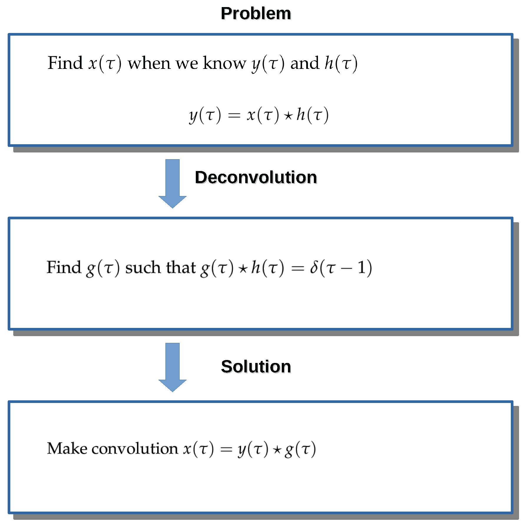
4. Mellin Deconvolution Problem

Consider a scale-invariant system with a transfer function $H\left(\nu \right)$ and input signal $x\left(\tau \right)$. The usual way to find the output signal $y\left(\tau \right)$ (response of a system) is by means of the convolution

$$y\left(\tau \right)=x\left(\tau \right)\star h\left(\tau \right),$$

(24)

where $h\left(\tau \right)={\mathcal{M}}^{-1}\left[H\left(\nu \right)\right]$ is the impulse response. The procedure of finding the output signal is well systematized; see [19]. Now, consider that we have a system where we know either the input-output signals or the transfer function and output signal. In the first case, we need to find the transfer function $H\left(\nu \right)$ (identification problem), and in the second case we need to find input signal $x\left(\tau \right)$ (deconvolution problem, see Figure 2), respectively. These problems are much more generally in their resolution, and they are not systematized. Here, we deal with the deconvolution problem. The deconvolution problem can be posed as follows: suppose that in (24) we found $g\left(\tau \right)$ such that $g\left(\tau \right)\star h\left(\tau \right)=\delta (\tau -1)$; then, the input signal $x\left(\tau \right)$ can be described as the convolution

$$x\left(\tau \right)=y\left(\tau \right)\star g\left(\tau \right).$$

When $H\left(\nu \right)$ is an unfavorable function, the deconvolution problem can be related to the class of so-called ill-posed problems [38].

If we consider that $g\left(\tau \right)$ and $h\left(\tau \right)$ are convolutionally inverse; then,

$$G\left(\nu \right)·H\left(\nu \right)=1.$$

Definition 3.

Let $a_k$, $k=k_0,k_0+1,\cdots$, $k_0\in {\mathbb{N}}_0$, be a discrete-time function of exponential order, for $k>K\in \mathbb{N}$ and $\alpha >0$. We define the α-logarithm power series of order $k_0$ by

$$g\left(\tau \right)=\sum _{k=k_0}^{\infty }{a}_k{\displaystyle \frac{{ln}^{k\alpha -1}\left(\tau \right)}{\Gamma \left(k\alpha \right)}}\epsilon (\tau -1).$$

(25)

and the $(\alpha ,\beta )$-logarithm power series by

$$g\left(\tau \right)=\sum _{k=k_0}^{\infty }{a}_k{\displaystyle \frac{{ln}^{\beta +k\alpha -1}\left(\tau \right)}{\Gamma (\beta +k\alpha )}}\epsilon (\tau -1),\beta >0.$$

Their Mellin transforms are

$$G\left(\nu \right)=\sum _{k=k_0}^{\infty }{a}_k{\nu }^{-k\alpha },$$

and

$$G\left(\nu \right)={\nu }^{-\beta }\sum _{k=k_0}^{\infty }{a}_k{\nu }^{-k\alpha },$$

respectively. These series converge when $\Re \left(\nu \right)>\gamma$, where γ depends on the sequence $a_k$.

Remark 3.

If, in Definition 3, we allow $k_0\in \mathbb{Z}$, then we obtain a α-logarithm Laurent series. We denote by $\mathcal{F}$ the vector space generated by an α-logarithm Laurent series using the usual addition and scalar product. Moreover, if we incorporate the multiplication of two series by means of the Cauchy product using the Mellin convolution, then in [39] it is proven that $\mathcal{F}$ is a field. This is an important result since it would tell us that any Laurent series in $\mathcal{F}$ has its convolutionally inverse in $\mathcal{F}$. The proof of this fact does not explicitly show us the convolutionally inverse partner.

In [10], it is shown that the convolution of two functions of the type (10) can be rewritten as a linear combination of functions of the same type. This is, for ${\gamma }_1\ne {\gamma }_2$,

$${\mathcal{E}}_{{\gamma }_1,0}\left(\tau \right)\star {\mathcal{E}}_{{\gamma }_2,0}\left(\tau \right)={\displaystyle \frac{{\mathcal{E}}_{{\gamma }_1,0}\left(\tau \right)-{\mathcal{E}}_{{\gamma }_2,0}\left(\tau \right)}{{\gamma }_1-{\gamma }_2}},$$

(26)

and

$$\begin{array}{cc}\hfill {\mathcal{E}}_{{\gamma }_1,m}\left(\tau \right)\star {\mathcal{E}}_{{\gamma }_2,n}\left(\tau \right)=\sum _{l=0}^m{\displaystyle \frac{\left(\genfrac{}{}{0pt}{}{n+l}{l}\right){(-1)}^l}{{({\gamma }_1-{\gamma }_2)}^{1+n+l}}}& {\mathcal{E}}_{{\gamma }_1,m-l}\left(\tau \right)+\sum _{k=0}^n{\displaystyle \frac{\left(\genfrac{}{}{0pt}{}{m+k}{k}\right){(-1)}^k}{{({\gamma }_2-{\gamma }_1)}^{1+m+k}}}{\mathcal{E}}_{{\gamma }_2,n-k}\left(\tau \right).\hfill \end{array}$$

(27)

When ${\gamma }_1={\gamma }_2$, we have that

$${\mathcal{E}}_{\gamma ,m}\left(\tau \right)\star {\mathcal{E}}_{\gamma ,n}\left(\tau \right)={\mathcal{E}}_{\gamma ,m+n+1}\left(\tau \right).$$

(28)

As we already mentioned in Remark 3, finding convolutionally inverse pairs is not simple. Here, we advance on the topic.

We recall that [34]

$${\displaystyle \frac{{ln}^{-1}\left(\tau \right)}{\Gamma \left(0\right)}}\epsilon (\tau -1)=\delta (\tau -1).$$

(29)

Theorem 1.

Let $\gamma \in \mathbb{C}$, and $\alpha \in {\mathbb{R}}^{+}$. Consider the α–log-exponential monomial of order zero [10]

$${\mathcal{E}}_{\gamma ,0}\left(\tau \right)=\sum _{k=1}^{\infty }{\gamma }^{k-1}{\displaystyle \frac{{ln}^{k\alpha -1}\left(\tau \right)}{\Gamma \left(k\alpha \right)}}\epsilon (\tau -1).$$

Hence, the convolutionally inverse of ${\mathcal{E}}_{\gamma ,0}\left(\tau \right)$ is given by

$$h\left(\tau \right)=\left({\displaystyle \frac{{ln}^{-\alpha -1}\left(\tau \right)}{\Gamma (-\alpha )}}\epsilon (\tau -1)-\gamma {\displaystyle \frac{{ln}^{-1}\left(\tau \right)}{\Gamma \left(0\right)}}\epsilon (\tau -1)\right).$$

Moreover, the Sonin partner of ${\mathcal{E}}_{\gamma ,0}\left(\tau \right)$ is given by

$$\varphi \left(\tau \right)={\mathfrak{D}}_{s+}^{-1}\left(h\left(\tau \right)\right)={\displaystyle \frac{{ln}^{-\alpha }\left(\tau \right)}{\Gamma (-\alpha +1)}}\epsilon (\tau -1)-\gamma \epsilon (\tau -1),$$

and the Sonin partner of $h\left(\tau \right)$ is

$$\psi \left(\tau \right)={\mathfrak{D}}_{s+}^{-1}\left({\mathcal{E}}_{\gamma ,0}\left(\tau \right)\right)=\sum _{k=1}^{\infty }{\gamma }^{k-1}{\displaystyle \frac{{ln}^{k\alpha }\left(\tau \right)}{\Gamma (k\alpha +1)}}\epsilon (\tau -1).$$

The proof of Theorem 1 is given in Appendix A.

We extend Theorem 1 to the case of $\alpha$–log-exponential monomials of order n. We no longer stop to find Sonin pairs due to the simplicity of their computation from convolutionally inverses. We denote

$$\begin{array}{cc}\hfill & {\left({\displaystyle \frac{{ln}^{-\alpha -1}\left(\tau \right)}{\Gamma (-\alpha )}}\epsilon (\tau -1)-\gamma {\displaystyle \frac{{ln}^{-1}\left(\tau \right)}{\Gamma \left(0\right)}}\epsilon (\tau -1)\right)}_{\star }^{n+1}=\hfill \\ \hfill & \underset{n+1-times}{\underbrace{\left({\displaystyle \frac{{ln}^{-\alpha -1}\left(\tau \right)}{\Gamma (-\alpha )}}\epsilon (\tau -1)-\gamma {\displaystyle \frac{{ln}^{-1}\left(\tau \right)}{\Gamma \left(0\right)}}\epsilon (\tau -1)\right)\star \cdots \star \left({\displaystyle \frac{{ln}^{-\alpha -1}\left(\tau \right)}{\Gamma (-\alpha )}}\epsilon (\tau -1)-\gamma {\displaystyle \frac{{ln}^{-1}\left(\tau \right)}{\Gamma \left(0\right)}}\epsilon (\tau -1)\right)}}.\hfill \end{array}$$

Theorem 2.

Let $n\in {\mathbb{N}}_0$, $\gamma \in \mathbb{C}$, and $\alpha \in {\mathbb{R}}^{+}$. Consider the α–log-exponential monomial of order n [10]:

$${\mathcal{E}}_{\gamma ,n}\left(\tau \right)=\sum _{k=n+1}^{\infty }\left({\displaystyle \genfrac{}{}{0pt}{}{k-1}{n}}\right){\gamma }^{k-n-1}{\displaystyle \frac{{ln}^{k\alpha -1}\left(\tau \right)}{\Gamma \left(k\alpha \right)}}\epsilon (\tau -1).$$

Hence, the convolutionally inverse of ${\mathcal{E}}_{\gamma ,n}\left(\tau \right)$ is given by

$$\begin{array}{cc}\hfill h\left(\tau \right)& ={\left({\displaystyle \frac{{ln}^{-\alpha -1}\left(\tau \right)}{\Gamma (-\alpha )}}\epsilon (\tau -1)-\gamma {\displaystyle \frac{{ln}^{-1}\left(\tau \right)}{\Gamma \left(0\right)}}\epsilon (\tau -1)\right)}_{\star }^{n+1}\hfill \\ \hfill & =\sum _{k=0}^{n+1}{(-1)}^k\left({\displaystyle \genfrac{}{}{0pt}{}{n+1}{k}}\right){\gamma }^k{\displaystyle \frac{{ln}^{(n+1-k)\alpha -1}\left(\tau \right)}{\Gamma \left(\right(n+1-k\left)\alpha \right)}}\epsilon (\tau -1).\hfill \end{array}$$

The proof of Theorem 2 is given in Appendix A.

Remark 4.

Let

$$g\left(\tau \right)=\sum _{k=0}^l{c}_k{\displaystyle \frac{{ln}^{-k\alpha -1}\left(\tau \right)}{\Gamma (-k\alpha )}}\epsilon (\tau -1),l\ge 1.$$

It is not difficult to see that $g\left(\tau \right)$ can be rewritten as

$$g\left(\tau \right)=c_l\prod _{k=0}^{l-1}{\left({\displaystyle \frac{{ln}^{-\alpha -1}\left(\tau \right)}{\Gamma (-\alpha )}}\epsilon (\tau -1)-r_k{\displaystyle \frac{{ln}^{-1}\left(\tau \right)}{\Gamma \left(0\right)}}\epsilon (\tau -1)\right)}_{\star },$$

where $r_k$s are the roots of the polynomial $x^l+{\displaystyle \frac{c_{l-1}}{c_l}}{x}^{l-1}+\cdots {\displaystyle \frac{c_1}{c_l}}x+{\displaystyle \frac{c_0}{c_l}}$.

We can go even further by finding the convolutionally inverse of a linear combination of $\alpha$–log-exponential monomials.

Remark 5.

Theorem 3 can be extended to the case of ${\sum }_{k=1}^N{c}_k{\mathcal{E}}_{{\gamma }_k,n_k}\left(\tau \right)$, but because the accounts are very cumbersome, we prefer not to present them here. Instead, we prefer to present some examples.

Theorem 3.

Let

$$g\left(\tau \right)=c_1{\mathcal{E}}_{{\gamma }_1,n_1}\left(\tau \right)+c_2{\mathcal{E}}_{{\gamma }_2,n_2}\left(\tau \right),{\gamma }_1\ne {\gamma }_2,$$

be a non-null function with $c_1,c_2\in \mathbb{R}$. Then, the convolutionally inverse of $g\left(\tau \right)$ is given by

$$\begin{array}{cc}\hfill h\left(\tau \right)& ={\left({\displaystyle \frac{{ln}^{-\alpha -1}\left(\tau \right)}{\Gamma (-\alpha )}}\epsilon (\tau -1)-{\gamma }_1{\displaystyle \frac{{ln}^{-1}\left(\tau \right)}{\Gamma \left(0\right)}}\epsilon (\tau -1)\right)}_{\star }^{n_1+1}\star \hfill \\ \hfill & {\left({\displaystyle \frac{{ln}^{-\alpha -1}\left(\tau \right)}{\Gamma (-\alpha )}}\epsilon (\tau -1)-{\gamma }_2{\displaystyle \frac{{ln}^{-1}\left(\tau \right)}{\Gamma \left(0\right)}}\epsilon (\tau -1)\right)}_{\star }^{n_2+1}\star {\displaystyle \frac{1}{R}}\prod _{k=0}^{M-1}{\left({\mathcal{E}}_{r_k,0}\left(\tau \right)\right)}_{\star }\hfill \end{array}$$

where $M=max(n_1+1,n_2+1)$; $r_k$s are the roots of the monic polynomial ${\displaystyle \frac{1}{R}}(c_1{(x-{\gamma }_2)}^{n_2+1}+c_2{(x-{\gamma }_1)}^{n_1+1})$ (we consider that $1/R$ makes the polynomial monic).

The proof of Theorem 3 is given in Appendix A.

The convolutionally inverse $h\left(\tau \right)$ presented in Theorem 3 can be simplified using the Formulas (A1), (26), and (27). We illustrate this in the following examples.

Example 4.

Let

$$g\left(\tau \right)=c_1{\mathcal{E}}_{{\gamma }_1,0}\left(\tau \right)+c_2{\mathcal{E}}_{{\gamma }_2,0}\left(\tau \right),{\gamma }_1\ne {\gamma }_2,$$

with constants $c_1,c_2$ and $c_1+c_2\ne 0$. From Theorem 3, we have that

$$\begin{array}{cc}\hfill h\left(\tau \right)& ={\left({\displaystyle \frac{{ln}^{-\alpha -1}\left(\tau \right)}{\Gamma (-\alpha )}}\epsilon (\tau -1)-{\gamma }_1{\displaystyle \frac{{ln}^{-1}\left(\tau \right)}{\Gamma \left(0\right)}}\epsilon (\tau -1)\right)}_{\star }\star \hfill \\ \hfill & {\left({\displaystyle \frac{{ln}^{-\alpha -1}\left(\tau \right)}{\Gamma (-\alpha )}}\epsilon (\tau -1)-{\gamma }_2{\displaystyle \frac{{ln}^{-1}\left(\tau \right)}{\Gamma \left(0\right)}}\epsilon (\tau -1)\right)}_{\star }\star {\displaystyle \frac{1}{R}}{\mathcal{E}}_{r_0,0}\left(\tau \right),\hfill \end{array}$$

where $R=c_1+c_2$ and $r_0={\displaystyle \frac{c_1{\gamma }_2+c_2{\gamma }_1}{c_1+c_2}}$. We can simplify $h\left(\tau \right)$ using (A1). We have that

$$\begin{array}{cc}\hfill & {\left({\displaystyle \frac{{ln}^{-\alpha -1}\left(\tau \right)}{\Gamma (-\alpha )}}\epsilon (\tau -1)-{\gamma }_1{\displaystyle \frac{{ln}^{-1}\left(\tau \right)}{\Gamma \left(0\right)}}\epsilon (\tau -1)\right)}_{\star }\star \hfill \\ \hfill & \phantom{gggggggggggg}{\left({\displaystyle \frac{{ln}^{-\alpha -1}\left(\tau \right)}{\Gamma (-\alpha )}}\epsilon (\tau -1)-{\gamma }_2{\displaystyle \frac{{ln}^{-1}\left(\tau \right)}{\Gamma \left(0\right)}}\epsilon (\tau -1)\right)}_{\star }=\hfill \\ \hfill & \phantom{ggggggggggggggg}{\displaystyle \frac{{ln}^{-2\alpha -1}\left(\tau \right)}{\Gamma (-2\alpha )}}\epsilon (\tau -1)-({\gamma }_1+{\gamma }_2){\displaystyle \frac{{ln}^{-\alpha -1}\left(\tau \right)}{\Gamma (-\alpha )}}\epsilon (\tau -1)+{\gamma }_1{\gamma }_2{\displaystyle \frac{{ln}^{-1}\left(\tau \right)}{\Gamma \left(0\right)}}\epsilon (\tau -1).\hfill \end{array}$$

Hence,

$$h\left(\tau \right)={\displaystyle \frac{{ln}^{-2\alpha -1}\left(\tau \right)}{\Gamma (-2\alpha )}}\epsilon (\tau -1)\star {\displaystyle \frac{1}{R}}{\mathcal{E}}_{r_0,0}\left(\tau \right)-{\displaystyle \frac{{\gamma }_1+{\gamma }_2}{R}}{\displaystyle \frac{{ln}^{-\alpha -1}\left(\tau \right)}{\Gamma (-\alpha )}}\epsilon (\tau -1)\star {\mathcal{E}}_{r_0,0}\left(\tau \right)+{\displaystyle \frac{{\gamma }_1{\gamma }_2}{R}}{\mathcal{E}}_{r_0,0}\left(\tau \right).$$

We recall that ${\mathcal{E}}_{r_0,0}\left(\tau \right)={\sum }_{k=1}^{\infty }{r}_0^{k-1}{\displaystyle \frac{{ln}^{k\alpha -1}\left(\tau \right)}{\Gamma \left(k\alpha \right)}}\epsilon (\tau -1)$. Finally,

$$\begin{array}{cc}\hfill h\left(\tau \right)={\displaystyle \frac{1}{R}}\sum _{k=1}^{\infty }{r}_0^{k-1}{\displaystyle \frac{{ln}^{(k-2)\alpha -1}\left(\tau \right)}{\Gamma \left(\right(k-2\left)\alpha \right)}}\epsilon (\tau -1)-{\displaystyle \frac{{\gamma }_1+{\gamma }_2}{R}}& \sum _{k=1}^{\infty }{r}_0^{k-1}{\displaystyle \frac{{ln}^{(k-1)\alpha -1}\left(\tau \right)}{\Gamma \left(\right(k-1\left)\alpha \right)}}\epsilon (\tau -1)+\hfill \\ \hfill & {\displaystyle \frac{{\gamma }_1{\gamma }_2}{R}}\sum _{k=1}^{\infty }{r}_0^{k-1}{\displaystyle \frac{{ln}^{k\alpha -1}\left(\tau \right)}{\Gamma \left(k\alpha \right)}}\epsilon (\tau -1).\hfill \end{array}$$

Example 5.

Consider

$$g\left(\tau \right)=-2{\mathcal{E}}_{{\gamma }_1,0}\left(\tau \right)+{\mathcal{E}}_{{\gamma }_2,1}\left(\tau \right),{\gamma }_1\ne {\gamma }_2.$$

Applying algebraic manipulation and Theorem 2, we can rewrite $g\left(\tau \right)$ as

$$\begin{array}{cc}\hfill g\left(\tau \right)& =-2{\mathcal{E}}_{{\gamma }_1,0}\left(\tau \right)\star {\mathcal{E}}_{{\gamma }_2,1}\left(\tau \right)\star {\left({\displaystyle \frac{{ln}^{-\alpha -1}\left(\tau \right)}{\Gamma (-\alpha )}}\epsilon (\tau -1)-{\gamma }_2{\displaystyle \frac{{ln}^{-1}\left(\tau \right)}{\Gamma \left(0\right)}}\epsilon (\tau -1)\right)}_{\star }^2\star \hfill \\ \hfill & \phantom{hhhhhhhhhhhh}{\mathcal{E}}_{{\gamma }_1,0}\left(\tau \right)\star {\mathcal{E}}_{{\gamma }_2,1}\left(\tau \right)\star \left({\displaystyle \frac{{ln}^{-\alpha -1}\left(\tau \right)}{\Gamma (-\alpha )}}\epsilon (\tau -1)-{\gamma }_1{\displaystyle \frac{{ln}^{-1}\left(\tau \right)}{\Gamma \left(0\right)}}\epsilon (\tau -1)\right)\hfill \\ \hfill & ={\mathcal{E}}_{{\gamma }_1,0}\left(\tau \right)\star {\mathcal{E}}_{{\gamma }_2,1}\left(\tau \right)\star \hfill \\ \hfill & \phantom{hhhhhhhhhhhh}\left(-2{\left({\displaystyle \frac{{ln}^{-\alpha -1}\left(\tau \right)}{\Gamma (-\alpha )}}\epsilon (\tau -1)-{\gamma }_2{\displaystyle \frac{{ln}^{-1}\left(\tau \right)}{\Gamma \left(0\right)}}\epsilon (\tau -1)\right)}_{\star }^2+\right.\hfill \\ \hfill & \phantom{hhhhhhhhhhhhhhhhhhhhhh}\left.{\left({\displaystyle \frac{{ln}^{-\alpha -1}\left(\tau \right)}{\Gamma (-\alpha )}}\epsilon (\tau -1)-{\gamma }_1{\displaystyle \frac{{ln}^{-1}\left(\tau \right)}{\Gamma \left(0\right)}}\epsilon (\tau -1)\right)}_{\phantom{\star }}^{\phantom{2}}\right).\hfill \end{array}$$

Observe that

$$\begin{array}{cc}\hfill -2& {\left({\displaystyle \frac{{ln}^{-\alpha -1}\left(\tau \right)}{\Gamma (-\alpha )}}\epsilon (\tau -1)-{\gamma }_2{\displaystyle \frac{{ln}^{-1}\left(\tau \right)}{\Gamma \left(0\right)}}\epsilon (\tau -1)\right)}_{\star }^2+\left({\displaystyle \frac{{ln}^{-\alpha -1}\left(\tau \right)}{\Gamma (-\alpha )}}\epsilon (\tau -1)-{\gamma }_1{\displaystyle \frac{{ln}^{-1}\left(\tau \right)}{\Gamma \left(0\right)}}\epsilon (\tau -1)\right)=\hfill \\ \hfill & -2\left({\displaystyle \frac{{ln}^{-2\alpha -1}\left(\tau \right)}{\Gamma (-2\alpha )}}\epsilon (\tau -1)-{\displaystyle \frac{(4{\gamma }_2+1)}{2}}{\displaystyle \frac{{ln}^{-\alpha -1}\left(\tau \right)}{\Gamma (-\alpha )}}\epsilon (\tau -1)+{\displaystyle \frac{(2{\gamma }_2^2+{\gamma }_1)}{2}}{\displaystyle \frac{{ln}^{-1}\left(\tau \right)}{\Gamma \left(0\right)}}\epsilon (\tau -1)\right)\hfill \end{array}$$

Let $r_1,r_2$ be the roots of the polynomial $x^2-{\displaystyle \frac{4{\gamma }_2+1}{2}}x+{\displaystyle \frac{2{\gamma }_2^2+{\gamma }_1}{2}}$. Hence,

$$\begin{array}{cc}\hfill -2\left({\displaystyle \frac{{ln}^{-2\alpha -1}\left(\tau \right)}{\Gamma (-2\alpha )}}\epsilon (\tau -1)-\right.& \left.{\displaystyle \frac{(4{\gamma }_2+1)}{2}}{\displaystyle \frac{{ln}^{-\alpha -1}\left(\tau \right)}{\Gamma (-\alpha )}}\epsilon (\tau -1)+{\displaystyle \frac{(2{\gamma }_2^2+{\gamma }_1)}{2}}{\displaystyle \frac{{ln}^{-1}\left(\tau \right)}{\Gamma \left(0\right)}}\epsilon (\tau -1)\right)\star \hfill \\ \hfill & \phantom{hhhhhhhhhhhhhhhhhh}\left({\displaystyle \frac{1}{-2}}{\mathcal{E}}_{r_1,0}\left(\tau \right)\star {\mathcal{E}}_{r_2,0}\left(\tau \right)\right)=\delta (\tau -1).\hfill \end{array}$$

Finally, the convolutionally inverse of $g\left(\tau \right)$ is given by

$$\begin{array}{cc}\hfill h\left(\tau \right)& =\left({\displaystyle \frac{{ln}^{-\alpha -1}\left(\tau \right)}{\Gamma (-\alpha )}}\epsilon (\tau -1)-{\gamma }_1{\displaystyle \frac{{ln}^{-1}\left(\tau \right)}{\Gamma \left(0\right)}}\epsilon (\tau -1)\right)\star \hfill \\ \hfill & \phantom{fffffff}{\left({\displaystyle \frac{{ln}^{-\alpha -1}\left(\tau \right)}{\Gamma (-\alpha )}}\epsilon (\tau -1)-{\gamma }_2{\displaystyle \frac{{ln}^{-1}\left(\tau \right)}{\Gamma \left(0\right)}}\epsilon (\tau -1)\right)}_{\star }^2\star \left({\displaystyle \frac{1}{-2}}{\mathcal{E}}_{r_1,0}\left(\tau \right)\star {\mathcal{E}}_{r_2,0}\left(\tau \right)\right).\hfill \end{array}$$

We can simplify these convolutions as follows. Observe that

$$\begin{array}{cc}\hfill & \left({\displaystyle \frac{{ln}^{-\alpha -1}\left(\tau \right)}{\Gamma (-\alpha )}}\epsilon (\tau -1)-{\gamma }_1{\displaystyle \frac{{ln}^{-1}\left(\tau \right)}{\Gamma \left(0\right)}}\epsilon (\tau -1)\right)\star {\left({\displaystyle \frac{{ln}^{-\alpha -1}\left(\tau \right)}{\Gamma (-\alpha )}}\epsilon (\tau -1)-{\gamma }_2{\displaystyle \frac{{ln}^{-1}\left(\tau \right)}{\Gamma \left(0\right)}}\epsilon (\tau -1)\right)}_{\star }^2=\hfill \\ \hfill & \phantom{fffffff}{\displaystyle \frac{{ln}^{-3\alpha -1}\left(\tau \right)}{\Gamma (-3\alpha )}}\epsilon (\tau -1)-(2{\gamma }_2+{\gamma }_1){\displaystyle \frac{{ln}^{-2\alpha -1}\left(\tau \right)}{\Gamma (-2\alpha )}}\epsilon (\tau -1)+\hfill \\ \hfill & \phantom{ffffhhhhhhhfff}({\gamma }_2^2+2{\gamma }_1{\gamma }_2){\displaystyle \frac{{ln}^{-\alpha -1}\left(\tau \right)}{\Gamma (-\alpha )}}\epsilon (\tau -1)-{\gamma }_1{\gamma }_2^2{\displaystyle \frac{{ln}^{-1}\left(\tau \right)}{\Gamma \left(0\right)}}\epsilon (\tau -1),\hfill \end{array}$$

and from (26)

$${\displaystyle \frac{1}{-2}}{\mathcal{E}}_{r_1,0}\left(\tau \right)\star {\mathcal{E}}_{r_2,0}\left(\tau \right)={\displaystyle \frac{{\mathcal{E}}_{r_1,0}\left(\tau \right)-{\mathcal{E}}_{r_2,0}\left(\tau \right)}{2(r_2-r_1)}}.$$

Therefore,

$$\begin{array}{cc}\hfill h\left(\tau \right)& ={\displaystyle \frac{1}{2(r_2-r_1)}}\left({\displaystyle \frac{{ln}^{-3\alpha -1}\left(\tau \right)}{\Gamma (-3\alpha )}}\epsilon (\tau -1)\star \left({\mathcal{E}}_{r_1,0}\left(\tau \right)-{\mathcal{E}}_{r_2,0}\left(\tau \right)\right)\right.\hfill \\ \hfill & \phantom{fffff}-(2{\gamma }_2+{\gamma }_1){\displaystyle \frac{{ln}^{-2\alpha -1}\left(\tau \right)}{\Gamma (-2\alpha )}}\epsilon (\tau -1)\star \left({\mathcal{E}}_{r_1,0}\left(\tau \right)-{\mathcal{E}}_{r_2,0}\left(\tau \right)\right)\hfill \\ \hfill & \phantom{fffffffff}+({\gamma }_2^2+2{\gamma }_1{\gamma }_2){\displaystyle \frac{{ln}^{-\alpha -1}\left(\tau \right)}{\Gamma (-\alpha )}}\epsilon (\tau -1)\star \left({\mathcal{E}}_{r_1,0}\left(\tau \right)-{\mathcal{E}}_{r_2,0}\left(\tau \right)\right)\hfill \\ \hfill & \left.\phantom{jjjjjjjjjjjjjjjjjjjjjjjjjjjjjjjjjjjjj{\displaystyle \frac{{ln}^{-3\alpha -1}\left(\tau \right)}{\Gamma (-3\alpha )}}}-{\gamma }_1{\gamma }_2^2\left({\mathcal{E}}_{r_1,0}\left(\tau \right)-{\mathcal{E}}_{r_2,0}\left(\tau \right)\right)\right),\hfill \end{array}$$

where the last convolutions are easy to calculate.

We now add an impulse to the $\alpha$–log-exponential monomial ${\mathcal{E}}_{\gamma ,n}\left(\tau \right)$.

Theorem 4.

Define

$$g\left(\tau \right)=\delta (\tau -1)+c_1{\mathcal{E}}_{\gamma ,n}\left(\tau \right),$$

with the constant $c_1$. Then, the convolutionally inverse of $g\left(\tau \right)$ is given by

$$\begin{array}{cc}\hfill h\left(\tau \right)& ={\left({\displaystyle \frac{{ln}^{-\alpha -1}\left(\tau \right)}{\Gamma (-\alpha )}}\epsilon (\tau -1)-\gamma {\displaystyle \frac{{ln}^{-1}\left(\tau \right)}{\Gamma \left(0\right)}}\epsilon (\tau -1)\right)}_{\star }^{n+1}\star \prod _{k=0}^n{\mathcal{E}}_{r_k,0}\left(\tau \right),\hfill \end{array}$$

where $r_k$s are the roots of the polynomial ${(x-\gamma )}^{n+1}+c_1$.

The proof of Theorem 4 is given in Appendix A.

We solve another example.

Example 6.

Let

$$g\left(\tau \right)=\delta (\tau -1)+c_1{\mathcal{E}}_{\gamma ,0}\left(\tau \right),$$

with the constant $c_1$. From Theorem 2, we know that

$${\mathcal{E}}_{\gamma ,0}\left(\tau \right)\star \left({\displaystyle \frac{{ln}^{-\alpha -1}\left(\tau \right)}{\Gamma (-\alpha )}}\epsilon (\tau -1)-\gamma {\displaystyle \frac{{ln}^{-1}\left(\tau \right)}{\Gamma \left(0\right)}}\epsilon (\tau -1)\right)=\delta (\tau -1).$$

We recall that $\delta (\tau -1)={\displaystyle \frac{{ln}^{-1}\left(\tau \right)}{\Gamma \left(0\right)}}\epsilon (\tau -1)$. It follows that

$$\begin{array}{cc}\hfill g\left(\tau \right)& ={\mathcal{E}}_{\gamma ,0}\left(\tau \right)\star \left({\displaystyle \frac{{ln}^{-\alpha -1}\left(\tau \right)}{\Gamma (-\alpha )}}\epsilon (\tau -1)-\gamma {\displaystyle \frac{{ln}^{-1}\left(\tau \right)}{\Gamma \left(0\right)}}\epsilon (\tau -1)\right)+c_1{\mathcal{E}}_{\gamma ,0}\left(\tau \right)\hfill \\ \hfill & ={\mathcal{E}}_{\gamma ,0}\left(\tau \right)\star \left({\displaystyle \frac{{ln}^{-\alpha -1}\left(\tau \right)}{\Gamma (-\alpha )}}\epsilon (\tau -1)-(\gamma -c_1){\displaystyle \frac{{ln}^{-1}\left(\tau \right)}{\Gamma \left(0\right)}}\epsilon (\tau -1)\right).\hfill \end{array}$$

In this case, $r_0=\gamma -c_1$ is the root of the polynomial $x-(\gamma -c_1)$. So, the convolutionally inverse of $g\left(\tau \right)$ is given by

$$\begin{array}{cc}\hfill h\left(\tau \right)& =\left({\displaystyle \frac{{ln}^{-\alpha -1}\left(\tau \right)}{\Gamma (-\alpha )}}\epsilon (\tau -1)-\gamma {\displaystyle \frac{{ln}^{-1}\left(\tau \right)}{\Gamma \left(0\right)}}\epsilon (\tau -1)\right)\star {\mathcal{E}}_{\gamma -c_1,0}\left(\tau \right)\hfill \\ \hfill & =\sum _{k=1}^{\infty }{(\gamma -c_1)}^{k-1}{\displaystyle \frac{{ln}^{(k-1)\alpha -1}\left(\tau \right)}{\Gamma \left(\right(k-1\left)\alpha \right)}}\epsilon (\tau -1)-\gamma {\mathcal{E}}_{\gamma -c_1,0}\left(\tau \right)\hfill \\ \hfill & =\delta (\tau -1)+(\gamma -c_1){\mathcal{E}}_{\gamma -c_1,0}\left(\tau \right)-\gamma {\mathcal{E}}_{\gamma -c_1,0}\left(\tau \right)\hfill \\ \hfill & =\delta (\tau -1)-c_1{\mathcal{E}}_{\gamma -c_1,0}\left(\tau \right).\hfill \end{array}$$

Example 7.

Consider

$$\begin{array}{cc}\hfill g\left(\tau \right)& =\delta (\tau -1)+{\mathcal{E}}_{\gamma ,1}\left(\tau \right)\hfill \end{array}.$$

Then, from Theorem 2,

$${\mathcal{E}}_{\gamma ,1}\left(\tau \right)\star {\left({\displaystyle \frac{{ln}^{-\alpha -1}\left(\tau \right)}{\Gamma (-\alpha )}}\epsilon (\tau -1)-\gamma {\displaystyle \frac{{ln}^{-1}\left(\tau \right)}{\Gamma \left(0\right)}}\epsilon (\tau -1)\right)}_{\star }^2=\delta (\tau -1).$$

It follows that $g\left(\tau \right)$ can be decomposed into the following convolution:

$$g\left(\tau \right)={\mathcal{E}}_{\gamma ,1}\left(\tau \right)\star \left({\displaystyle \frac{{ln}^{-2\alpha -1}\left(\tau \right)}{\Gamma (-2\alpha )}}\epsilon (\tau -1)-2\gamma {\displaystyle \frac{{ln}^{-\alpha -1}\left(\tau \right)}{\Gamma (-\alpha )}}\epsilon (\tau -1)+({\gamma }^2+1){\displaystyle \frac{{ln}^{-1}\left(\tau \right)}{\Gamma \left(0\right)}}\epsilon (\tau -1)\right)$$

Suppose that $r_0,r_1$ are the roots of the polynomial $x^2-2\gamma x+{\gamma }^2+1$. Hence,

$$\begin{array}{cc}\hfill {\displaystyle \frac{{ln}^{-2\alpha -1}\left(\tau \right)}{\Gamma (-2\alpha )}}& \epsilon (\tau -1)-2\gamma {\displaystyle \frac{{ln}^{-\alpha -1}\left(\tau \right)}{\Gamma (-\alpha )}}\epsilon (\tau -1)+({\gamma }^2+1){\displaystyle \frac{{ln}^{-1}\left(\tau \right)}{\Gamma \left(0\right)}}\epsilon (\tau -1)=\hfill \\ \hfill & \left({\displaystyle \frac{{ln}^{-\alpha -1}\left(\tau \right)}{\Gamma (-\alpha )}}-r_0{\displaystyle \frac{{ln}^{-1}\left(\tau \right)}{\Gamma \left(0\right)}}\epsilon (\tau -1)\right)\star \left({\displaystyle \frac{{ln}^{-\alpha -1}\left(\tau \right)}{\Gamma (-\alpha )}}-r_1{\displaystyle \frac{{ln}^{-1}\left(\tau \right)}{\Gamma \left(0\right)}}\epsilon (\tau -1)\right).\hfill \end{array}$$

We recall that

$$\left({\displaystyle \frac{{ln}^{-\alpha -1}\left(\tau \right)}{\Gamma (-\alpha )}}-r_0{\displaystyle \frac{{ln}^{-1}\left(\tau \right)}{\Gamma \left(0\right)}}\epsilon (\tau -1)\right)\star {\mathcal{E}}_{r_0,0}\left(\tau \right)=\delta (\tau -1),$$

and

$$\left({\displaystyle \frac{{ln}^{-\alpha -1}\left(\tau \right)}{\Gamma (-\alpha )}}-r_1{\displaystyle \frac{{ln}^{-1}\left(\tau \right)}{\Gamma \left(0\right)}}\epsilon (\tau -1)\right)\star {\mathcal{E}}_{r_1,0}\left(\tau \right)=\delta (\tau -1).$$

This leads us to

$$\begin{array}{cc}\hfill & \left({\displaystyle \frac{{ln}^{-2\alpha -1}\left(\tau \right)}{\Gamma (-2\alpha )}}\epsilon (\tau -1)-2\gamma {\displaystyle \frac{{ln}^{-\alpha -1}\left(\tau \right)}{\Gamma (-\alpha )}}\epsilon (\tau -1)+{\gamma }^2{\displaystyle \frac{{ln}^{-1}\left(\tau \right)}{\Gamma \left(0\right)}}\epsilon (\tau -1)\right)\star \hfill \\ \hfill & \phantom{hhhhhhhhhhhhhhhhhhhhhhhhhhhh}{\mathcal{E}}_{r_0,0}\left(\tau \right)\star {\mathcal{E}}_{r_1,0}\left(\tau \right)=\delta (\tau -1).\hfill \end{array}$$

Hence, the convolutionally inverse of $g\left(\tau \right)$ is given by

$$h\left(\tau \right)=\left({\displaystyle \frac{{ln}^{-2\alpha -1}\left(\tau \right)}{\Gamma (-2\alpha )}}\epsilon (\tau -1)-2\gamma {\displaystyle \frac{{ln}^{-\alpha -1}\left(\tau \right)}{\Gamma (-\alpha )}}\epsilon (\tau -1)+{\gamma }^2{\displaystyle \frac{{ln}^{-1}\left(\tau \right)}{\Gamma \left(0\right)}}\epsilon (\tau -1)\right)\star {\mathcal{E}}_{r_0,0}\left(\tau \right)\star {\mathcal{E}}_{r_1,0}\left(\tau \right).$$

If we suppose that $r_1\ne r_2$, then, from (26), ${\mathcal{E}}_{r_0,0}\left(\tau \right)\star {\mathcal{E}}_{r_1,0}\left(\tau \right)={\displaystyle \frac{{\mathcal{E}}_{r_0,0}\left(\tau \right)-{\mathcal{E}}_{r_1,0}\left(\tau \right)}{r_0-r_1}}$. It follows that

$$\begin{array}{cc}\hfill h\left(\tau \right)& ={\displaystyle \frac{1}{r_0-r_1}}\left({\displaystyle \frac{{ln}^{-2\alpha -1}\left(\tau \right)}{\Gamma (-2\alpha )}}\epsilon (\tau -1)\star {\mathcal{E}}_{r_0,0}\left(\tau \right)-2\gamma {\displaystyle \frac{{ln}^{-\alpha -1}\left(\tau \right)}{\Gamma (-\alpha )}}\epsilon (\tau -1)\star {\mathcal{E}}_{r_0,0}\left(\tau \right)+{\gamma }^2{\mathcal{E}}_{r_0,0}\left(\tau \right)\right)-\hfill \\ \hfill & \phantom{gg}{\displaystyle \frac{1}{r_0-r_1}}\left({\displaystyle \frac{{ln}^{-2\alpha -1}\left(\tau \right)}{\Gamma (-2\alpha )}}\epsilon (\tau -1)\star {\mathcal{E}}_{r_1,0}\left(\tau \right)-2\gamma {\displaystyle \frac{{ln}^{-\alpha -1}\left(\tau \right)}{\Gamma (-\alpha )}}\epsilon (\tau -1)\star {\mathcal{E}}_{r_1,0}\left(\tau \right)+{\gamma }^2{\mathcal{E}}_{r_1,0}\left(\tau \right)\right).\hfill \end{array}$$

Simplifying, we obtain

$$\begin{array}{cc}\hfill h\left(\tau \right)& ={\displaystyle \frac{1}{r_0-r_1}}\left(\sum _{k=1}^{\infty }(r_0^{k-1}-r_1^{k-1}){\displaystyle \frac{{ln}^{(k-2)\alpha -1}\left(\tau \right)}{\Gamma \left(\right(k-2\left)\alpha \right)}}\epsilon (\tau -1)-\right.\hfill \\ \hfill & \phantom{gggggggggggggg}2\gamma \sum _{k=1}^{\infty }(r_0^{k-1}-r_1^{k-1}){\displaystyle \frac{{ln}^{(k-1)\alpha -1}\left(\tau \right)}{\Gamma \left(\right(k-1\left)\alpha \right)}}\epsilon (\tau -1)+\hfill \\ \hfill & \phantom{ggggggggggggggggggg}\left.{\gamma }^2\sum _{k=1}^{\infty }(r_0^{k-1}-r_1^{k-1}){\displaystyle \frac{{ln}^{k\alpha -1}\left(\tau \right)}{\Gamma \left(k\alpha \right)}}\epsilon (\tau -1)\right).\hfill \end{array}$$

We can also add a linear combination of terms of the type ${\displaystyle \frac{{ln}^{k\alpha -1}\left(\tau \right)}{\Gamma \left(k\alpha \right)}}\epsilon (\tau -1)$, $k\in {\mathbb{Z}}^{-}$. The following is an example of how to do this.

Example 8.

Let us consider

$$g\left(\tau \right)={\displaystyle \frac{{ln}^{-\alpha -1}\left(\tau \right)}{\Gamma (-\alpha )}}\epsilon (\tau -1)+\delta (\tau -1)+c_1{\mathcal{E}}_{\gamma ,0}\left(\tau \right),$$

where $c_1$ is a real constant. It is not difficult to see that

$${\mathcal{E}}_{\gamma ,0}\left(\tau \right)\star \left({\displaystyle \frac{{ln}^{-\alpha -1}\left(\tau \right)}{\Gamma (-\alpha )}}\epsilon (\tau -1)-\gamma {\displaystyle \frac{{ln}^{-1}\left(\tau \right)}{\Gamma \left(0\right)}}\epsilon (\tau -1)\right)=\delta (\tau -1),$$

and

$${\mathcal{E}}_{\gamma ,0}\left(\tau \right)\star \left({\displaystyle \frac{{ln}^{-2\alpha -1}\left(\tau \right)}{\Gamma (-2\alpha )}}\epsilon (\tau -1)-\gamma {\displaystyle \frac{{ln}^{-\alpha -1}\left(\tau \right)}{\Gamma (-\alpha )}}\epsilon (\tau -1)\right)={\displaystyle \frac{{ln}^{-\alpha -1}\left(\tau \right)}{\Gamma (-\alpha )}}\epsilon (\tau -1).$$

Hence,

$$g\left(\tau \right)={\mathcal{E}}_{\gamma ,0}\left(\tau \right)\star \left({\displaystyle \frac{{ln}^{-2\alpha -1}\left(\tau \right)}{\Gamma (-2\alpha )}}\epsilon (\tau -1)+(1-\gamma ){\displaystyle \frac{{ln}^{-\alpha -1}\left(\tau \right)}{\Gamma (-\alpha )}}\epsilon (\tau -1)+(c_1-\gamma )\delta (\tau -1)\right).$$

Let $r_0,r_1$ be the roots of polynomial $x^2+(1+\gamma )x+c_1-\gamma$. Hence,

$$\begin{array}{cc}\hfill {\displaystyle \frac{{ln}^{-2\alpha -1}\left(\tau \right)}{\Gamma (-2\alpha )}}\epsilon (\tau -1)& +(1-\gamma ){\displaystyle \frac{{ln}^{-\alpha -1}\left(\tau \right)}{\Gamma (-\alpha )}}\epsilon (\tau -1)+(c_1-\gamma )\delta (\tau -1)=\hfill \\ \hfill & \left({\displaystyle \frac{{ln}^{-\alpha -1}\left(\tau \right)}{\Gamma (-\alpha )}}\epsilon (\tau -1)-r_0\delta (\tau -1)\right)\star \left({\displaystyle \frac{{ln}^{-\alpha -1}\left(\tau \right)}{\Gamma (-\alpha )}}\epsilon (\tau -1)-r_1\delta (\tau -1)\right).\hfill \end{array}$$

Suppose that $r_0\ne r_1$. Therefore,

$$\begin{array}{cc}\hfill h\left(\tau \right)& =\left({\displaystyle \frac{{ln}^{-\alpha -1}\left(\tau \right)}{\Gamma (-\alpha )}}\epsilon (\tau -1)-\gamma {\displaystyle \frac{{ln}^{-1}\left(\tau \right)}{\Gamma \left(0\right)}}\epsilon (\tau -1)\right)\star {\mathcal{E}}_{r_0,0}\left(\tau \right)\star {\mathcal{E}}_{r_1,0}\left(\tau \right)\hfill \\ \hfill & =\left({\displaystyle \frac{{ln}^{-\alpha -1}\left(\tau \right)}{\Gamma (-\alpha )}}\epsilon (\tau -1)-\gamma {\displaystyle \frac{{ln}^{-1}\left(\tau \right)}{\Gamma \left(0\right)}}\epsilon (\tau -1)\right)\star \left({\displaystyle \frac{{\mathcal{E}}_{r_0,0}\left(\tau \right)-{\mathcal{E}}_{r_1,0}\left(\tau \right)}{r_0-r_1}}\right)\hfill \\ \hfill & ={\displaystyle \frac{{ln}^{-\alpha -1}\left(\tau \right)}{\Gamma (-\alpha )}}\epsilon (\tau -1)\star \left({\displaystyle \frac{{\mathcal{E}}_{r_0,0}\left(\tau \right)-{\mathcal{E}}_{r_1,0}\left(\tau \right)}{r_0-r_1}}\right)-\gamma \left({\displaystyle \frac{{\mathcal{E}}_{r_0,0}\left(\tau \right)-{\mathcal{E}}_{r_1,0}\left(\tau \right)}{r_0-r_1}}\right)\hfill \\ \hfill & ={\displaystyle \frac{1}{r_0-r_1}}\left({\displaystyle \frac{{ln}^{-\alpha -1}\left(\tau \right)}{\Gamma (-\alpha )}}\epsilon (\tau -1)\star {\mathcal{E}}_{r_0,0}\left(\tau \right)-{\displaystyle \frac{{ln}^{-\alpha -1}\left(\tau \right)}{\Gamma (-\alpha )}}\epsilon (\tau -1)\star {\mathcal{E}}_{r_1,0}\left(\tau \right)\right)-\hfill \\ \hfill & \phantom{hhhhhhhhhhhhhhhhhhhhhhhhhhhhhhhhhhhhhhhhhhhhhh}\gamma \left({\displaystyle \frac{{\mathcal{E}}_{r_0,0}\left(\tau \right)-{\mathcal{E}}_{r_1,0}\left(\tau \right)}{r_0-r_1}}\right)\hfill \end{array}$$

Observe that

$${\displaystyle \frac{{ln}^{-\alpha -1}\left(\tau \right)}{\Gamma (-\alpha )}}\epsilon (\tau -1)\star {\mathcal{E}}_{r_0,0}\left(\tau \right)=\delta (\tau -1)+r_0{\mathcal{E}}_{r_0,0}\left(\tau \right).$$

Finally, the convolutionally inverse of $g\left(\tau \right)$ is

$$\begin{array}{cc}\hfill h\left(\tau \right)& ={\displaystyle \frac{1}{r_0-r_1}}\left(r_0{\mathcal{E}}_{r_0,0}\left(\tau \right)-r_1{\mathcal{E}}_{r_1,0}\left(\tau \right)\right)-\gamma \left({\displaystyle \frac{{\mathcal{E}}_{r_0,0}\left(\tau \right)-{\mathcal{E}}_{r_1,0}\left(\tau \right)}{r_0-r_1}}\right)\hfill \\ \hfill & ={\displaystyle \frac{r_0-\gamma }{r_0-r_1}}{\mathcal{E}}_{r_0,0}\left(\tau \right)-{\displaystyle \frac{r_1-\gamma }{r_0-r_1}}{\mathcal{E}}_{r_1,0}\left(\tau \right).\hfill \end{array}$$

These results can be extended to the case ${\sum }_{k=0}^M{\displaystyle \frac{{ln}^{-k\alpha -1}\left(\tau \right)}{\Gamma (-k\alpha )}}\epsilon (\tau -1)+{\sum }_{k=1}^N{c}_k{\mathcal{E}}_{{\gamma }_k,n_k}\left(\tau \right)$, but we do not develop it.

In a straightforward way, we can find the convolutionally inverse pairs of any series of the type (25). We present this in the next theorem.

Theorem 5.

Let $g\left(\tau \right)$ be an α-logarithm power series as in (25) and $h\left(\tau \right)$ the α-logarithm Laurent series

$$h\left(\tau \right)={\mathcal{M}}^{-1}\left[H\left(\nu \right)\right]=\sum _{k=m_0}^{\infty }{b}_k{\displaystyle \frac{{ln}^{k\alpha -1}\left(\tau \right)}{\Gamma \left(k\alpha \right)}}\epsilon (\tau -1),m_0\in \mathbb{Z}.$$

These series are convolutionally inverses if and only if

$$\sum _{m=0}^n{a}_{m+m_0}{b}_{n-m-m_0}={\delta }_n,n\ge 0,$$

where ${\delta }_n$, $n\in \mathbb{Z}$, is the Kronecker delta.

The proof of Theorem 5 is given in Appendix A. In the proof of Theorem 5, a very important fact is deduced: $k_0=-m_0$.

Example 9.

Let $N\in \mathbb{N}$. We know that for $\tau >1$, $g\left(\tau \right)$ satisfies

$$g\left(\tau \right)={\tau }^N=\sum _{n=0}^{\infty }{\displaystyle \frac{N^n}{n!}}{ln}^n\left(\tau \right)\epsilon (\tau -1).$$

Then,

$$\begin{array}{cc}\hfill G\left(\nu \right)& =\sum _{n=0}^{\infty }{N}^n\mathcal{M}\left[{\displaystyle \frac{{ln}^n\left(\tau \right)}{n!}}\epsilon (\tau -1)\right]\hfill \\ \hfill & =\sum _{n=0}^{\infty }{N}^n{\nu }^{-n}\hfill \\ \hfill & ={\displaystyle \frac{\nu }{\nu -N}},\hfill \end{array}$$

when $\Re \left({\displaystyle \frac{N}{\nu }}\right)<1$. We can compute the coefficients of convolutionally inverse series of (30) using (A3). In this case, $k_0=1$ and then $m_0=-1.$ It follows that $h_{-1}=1$, $h_0=-N$, and $h_n=0$ for $n\ge 1$. Therefore,

$$h\left(\tau \right)={\displaystyle \frac{{ln}^{-2}\left(\tau \right)}{\Gamma (-1)}}\epsilon (\tau -1)-N\delta (\tau -1).$$

(30)

We conclude with the following theorem whose proof is found in Appendix A.

Theorem 6.

Let

$$g_{\beta }\left(\tau \right)=\sum _{k=0}^{\infty }{a}_k{\displaystyle \frac{{ln}^{k\alpha +\beta -1}\left(\tau \right)}{\Gamma (k\alpha +\beta )}}\epsilon (\tau -1),\alpha \ge 0,0<\beta <1.$$

Then, there exists a regular Sonin partner of $g_{\beta }\left(\tau \right)$ given by

$${\varphi }_{\beta }\left(\tau \right)={ln}^{-\beta }\left(\tau \right)\sum _{k=0}^{\infty }{b}_k{\displaystyle \frac{{ln}^{k\alpha }\left(\tau \right)}{\Gamma (k\alpha -\beta )}}\epsilon (\tau -1).$$

5. Scale-Invariant Linear Systems

5.1. Integer-Order Scale-Invariant Linear Systems

Let $A\left(z\right)={\sum }_{k=0}^N{a}_k{z}^k$ and $B\left(z\right)={\sum }_{k=0}^M{b}_k{z}^k$ be polynomials with real coefficients of degree N and M, respectively. Suppose that the polynomials have no common roots. The systems described as

$$A\left({\mathcal{D}}_{s+}\right)y\left(\tau \right)=B\left({\mathcal{D}}_{s+}\right)x\left(\tau \right),\tau \ge 1,$$

(31)

where ${\mathcal{D}}_{s+}$ means the scale-derivative [9], are known as dilation-invariant autoregressive-moving average DI-ARMA($N,M$). The corresponding transfer function is

$$G\left(\nu \right)={\displaystyle \frac{{\sum }_{k=0}^M{b}_k{\nu }^k}{{\sum }_{k=0}^N{a}_k{\nu }^k}}.$$

Example 10.

Consider $G\left(\nu \right)={\displaystyle \frac{b_1\nu }{a_1\nu +a_0}},$ with $a_1,a_0,b_1\in {\mathbb{R}}^{+}$. Observe that $G\left(\nu \right)$ can be rewritten as

$$G\left(\nu \right)={\displaystyle \frac{b_1}{a_1}}-{\displaystyle \frac{\frac{b_1{a}_0}{a_1^2}}{v+\frac{a_0}{a_1}}}.$$

Then, the impulse response is

$$g\left(\tau \right)={\displaystyle \frac{b_1}{a_1}}\delta (\tau -1)-{\displaystyle \frac{b_1{a}_0}{a_1^2}}{\tau }^{-{\displaystyle \frac{a_0}{a_1}}}\epsilon (\tau -1).$$

The inverse system is represented by $H\left(\nu \right)={\displaystyle \frac{a_1\nu +a_0}{b_1\nu }}$. $H\left(\nu \right)$ can be rewritten as

$$H\left(\nu \right)={\displaystyle \frac{a_1}{b_1}}+{\displaystyle \frac{a_0}{b_1}}{\displaystyle \frac{1}{\nu }}.$$

So, the impulse response of the inverse system is

$$h\left(\tau \right)={\displaystyle \frac{a_1}{b_1}}\delta (\tau -1)+{\displaystyle \frac{a_0}{b_1}}\epsilon (\tau -1).$$

To verify the previous result, we only need to check that $g\left(\tau \right)\star h\left(\tau \right)=\delta (\tau -1)$. For this, it is enough to note that $\delta (\tau -1)$ is the identity element of the Mellin convolution and

$${\displaystyle \frac{b_1{a}_0}{a_1^2}}{\tau }^{-{\displaystyle \frac{a_0}{a_1}}}\epsilon (\tau -1)\star {\displaystyle \frac{a_0}{b_1}}\epsilon (\tau -1)={\displaystyle \frac{a_0}{a_1}}+{\displaystyle \frac{a_0}{a_1}}{\tau }^{-{\displaystyle \frac{a_0}{a_1}}}.$$

5.2. Non-Integer-Order Commensurate Scale-Invariant Linear Systems

The non-integer-order commensurate case in a DI-ARMA($N,N$) system can be easily treated. We only need to replace $\nu$ by ${\nu }^{\alpha }$ with $0\le \alpha \le 1$. The transfer function is

$$G\left(\nu \right)={\displaystyle \frac{{\sum }_{k=0}^N{b}_k{\nu }^{k\alpha }}{{\sum }_{k=0}^N{a}_k{\nu }^{k\alpha }}}={\displaystyle \frac{b_N}{a_N}}\prod _{k=1}^N{\displaystyle \frac{{\nu }^{\alpha }-z_k}{{\nu }^{\alpha }-p_k}},$$

where $z_k$ and $p_k$ are the pseudo-zeroes and -poles [40]. Let $N_p$, $N_z$ be the number of pseudo-poles and pseudo-zeros, respectively; and let $n_k+1$, $m_k+1$ be their respective multiplicity. Applying partial fraction decomposition, we have that

$$G\left(\nu \right)=A_0+\sum _{k=1}^{N_p}{\displaystyle \frac{A_k}{{({\nu }^{\alpha }-p_k)}^{n_k}}},$$

where $A_0=b_N/a_N$. The inverse system can be characterized as follows:

$$H\left(\nu \right)=B_0+\sum _{m=1}^{N_z}{\displaystyle \frac{B_m}{{({\nu }^{\alpha }-z_m)}^{n_m}}}.$$

where $B_m$ represents the residues at the pseudo-zeroes $z_k$. The condition $A_0{B}_0=1$ is also satisfied.

We invert each partial fraction following a procedure similar to that in the previous subsection. From (11) and (29), we have that

$$g\left(\tau \right)=A_0\delta (\tau -1)+\sum _{k=1}^{N_p}{A}_k{\mathcal{E}}_{p_k,n_k-1}\left(\tau \right),$$

and

$$h\left(\tau \right)=B_0\delta (\tau -1)+\sum _{m=1}^{N_z}{B}_m{\mathcal{E}}_{z_m,n_m-1}\left(\tau \right).$$

If we define

$${\mathcal{S}}_{\gamma ,n}\left(\tau \right)={\mathcal{E}}_{\gamma ,n}\left(\tau \right)\star \epsilon (\tau -1)=\sum _{k=n+1}^{\infty }\left({\displaystyle \genfrac{}{}{0pt}{}{k-1}{n}}\right){\gamma }^{k-n-1}{\displaystyle \frac{{ln}^{k\alpha }\left(\tau \right)}{\Gamma (k\alpha +1)}}\epsilon (\tau -1).$$

then the step response is given by

$$\psi \left(\tau \right)=A_0\delta (\tau -1)+\sum _{k=1}^{N_p}{A}_k{\mathcal{S}}_{p_k,n_k-1}\left(\tau \right).$$

The computation of $h\left(\tau \right)$ is similar. The $\alpha$–log-exponential monomial ${\mathcal{E}}_{\gamma ,n}\left(\tau \right)$ has the same convergence properties of the Mittag–Leffler function [41].

Example 11.

Consider $G\left(\nu \right)={\displaystyle \frac{b_1{\nu }^{\alpha }}{a_1{\nu }^{\alpha }+a_0}}$, with $a_1,a_0,b_1\in {\mathbb{R}}^{+}$. Observe that $G\left(\nu \right)$ can be rewritten as

$$G\left(\nu \right)={\displaystyle \frac{b_1}{a_1}}-{\displaystyle \frac{\frac{b_1{a}_0}{a_1^2}}{v^{\alpha }+\frac{a_0}{a_1}}}.$$

Observe that

$${\displaystyle \frac{1}{v^{\alpha }+\frac{a_0}{a_1}}}=\sum _{k=0}^{\infty }{\left(-{\displaystyle \frac{a_0}{a_1}}\right)}^k{\nu }^{-(k+1)\alpha },\Re \left(\nu \right)>\left|{\displaystyle \frac{a_0}{a_1}}\right|.$$

It follows that

$$\begin{array}{cc}\hfill g\left(\tau \right)& ={\displaystyle \frac{b_1}{a_1}}\delta (\tau -1)-{\displaystyle \frac{b_1{a}_0}{a_1^2}}\sum _{k=0}^{\infty }{\left(-{\displaystyle \frac{a_0}{a_1}}\right)}^k{\displaystyle \frac{{ln}^{(k+1)\alpha -1}\left(\tau \right)}{\Gamma \left(\right(k+1\left)\alpha \right)}}\epsilon (\tau -1)\hfill \\ \hfill & ={\displaystyle \frac{b_1}{a_1}}\delta (\tau -1)-{\displaystyle \frac{b_1{a}_0}{a_1^2}}{\mathcal{E}}_{-{\displaystyle \frac{a_0}{a_1}},0}\left(\tau \right).\hfill \end{array}$$

The inverse system is represented by $H\left(\nu \right)={\displaystyle \frac{a_1{\nu }^{\alpha }+a_0}{b_1{\nu }^{\alpha }}}$. $H\left(\nu \right)$ can be rewritten as

$$H\left(\nu \right)={\displaystyle \frac{a_1}{b_1}}+{\displaystyle \frac{a_0}{b_1}}{\displaystyle \frac{1}{{\nu }^{\alpha }}}.$$

So, the impulse response of the inverse system is

$$h\left(\tau \right)={\displaystyle \frac{a_1}{b_1}}\delta (\tau -1)+{\displaystyle \frac{a_0}{b_1}}{\displaystyle \frac{{ln}^{\alpha -1}\left(\tau \right)}{\Gamma \left(\alpha \right)}}\epsilon (\tau -1).$$

6. Conclusions

A study of the Mellin convolution is performed by means of its deconvolution. The $\alpha$–log-exponential monomials serve as the basis for the deconvolution process. The Sonin-like conditions for the Mellin convolution are established, and it is shown that the deconvolution process serves to generate Sonin pairs. Applications to scale-invariant linear systems are then studied.

References

1. Hirschman, I.; Widder, D. The Convolution Transform; Courier Corporation: North Chelmsford, MA, USA, 2012. [Google Scholar]
2. Domínguez, A. A History of the Convolution Operation [Retrospectroscope]. IEEE Pulse 2015, 6, 38–49. [Google Scholar] [CrossRef] [PubMed]
3. Roberts, M.J. Signals and Systems: Analysis Using Transform Methods and Matlab; McGraw-Hill: New York, NY, USA, 2003. [Google Scholar]
4. Ortigueira, M.D.; Machado, J.T. The 21st century systems: An updated vision of continuous-time fractional models. IEEE Circuits Syst. Mag. 2022, 22, 36–56. [Google Scholar] [CrossRef]
5. Braccini, C.; Gambardella, G. Form-invariant linear filtering: Theory and applications. IEEE Trans. Acoust. Speech Signal Process. 1986, 34, 1612–1628. [Google Scholar] [CrossRef]
6. Yazici, B.; Kashyap, R.L. A class of second-order stationary self-similar processes for 1/f phenomena. IEEE Trans. Signal Process. 1997, 45, 396–410. [Google Scholar] [CrossRef]
7. Cohen, L. The scale representation. IEEE Trans. Signal Process. 1993, 41, 3275–3292. [Google Scholar] [CrossRef]
8. Ortigueira, M.D. On the fractional linear scale invariant systems. IEEE Trans. Signal Process. 2010, 58, 6406–6410. [Google Scholar] [CrossRef]
9. Ortigueira, M.; Bohannan, G. Fractional scale calculus: Hadamard vs. Liouville. Fractal Fract. 2023, 7, 296. [Google Scholar] [CrossRef]
10. Bengochea, G.; Ortigueira, M. An Operational Approach to Fractional Scale-Invariant Linear Systems. Fractal Fract. 2023, 7, 524. [Google Scholar] [CrossRef]
11. Gupta, A.; Singh, P.; Aggarwal, P.; Joshi, S.D. Unified framework for linear scale invariant signals, systems, and transforms: A tutorial. Digit. Signal Process. 2025, 157, 104880. [Google Scholar] [CrossRef]
12. Grossmann, A.; Morlet, J. Decomposition of Hardy functions into square integrable wavelets of constant shape. SIAM J. Math. Anal. 1984, 15, 723–736. [Google Scholar] [CrossRef]
13. Mallat, S.G. Multiresolution Representations and Wavelets; University of Pennsylvania: Philadelphia, PA, USA, 1988. [Google Scholar]
14. Heil, C.E.; Walnut, D.F. Continuous and discrete wavelet transforms. SIAM Rev. 1989, 31, 628–666. [Google Scholar] [CrossRef]
15. Nottale, L. The theory of scale relativity. Int. J. Mod. Phys. A 1992, 7, 4899–4936. [Google Scholar] [CrossRef]
16. Nottale, L. Non-differentiable space-time and scale relativity. In Proceedings of the International Colloquium Geometrie au XXe Siecle, Paris, France, 24–29 September 2001. [Google Scholar]
17. Borgnat, P.; Amblard, P.O.; Flandrin, P. Scale invariances and Lamperti transformations for stochastic processes. J. Phys. A Math. Gen. 2005, 38, 2081. [Google Scholar] [CrossRef]
18. Butzer, P.; Jansche, S. A direct approach to the Mellin transform. J. Fourier Anal. Appl. 1997, 3, 325–376. [Google Scholar] [CrossRef]
19. Bertrand, J.; Bertrand, P.; Ovarlez, J. The Mellin transform. In The Transforms and Applications Handbook; CRC Press: Boca Raton, FL, USA, 1995. [Google Scholar]
20. Kim, H.; Cao, J.; Kim, J.; Zhang, W. A Mellin transform approach to pricing barrier options under stochastic elasticity of variance. Appl. Stoch. Models Bus. Ind. 2023, 39, 160–176. [Google Scholar] [CrossRef]
21. Fikioris, G. Mellin-Transform Method for Integral Evaluation: Introduction and Applications to Electromagnetics; Springer Nature: New York, NY, USA, 2022. [Google Scholar]
22. Shen, X.; Gamboa, J.; Hamidfar, T.; Shahriar, S. Investigation of frequency invariance in automated event recognition using resonant atomic media. In Proceedings of the Practical Holography XXXVIII: Displays, Materials, and Applications, San Francisco, CA, USA, 27 January–1 February 2024; Blanche, P.A.J., Lee, S.H., Eds.; International Society for Optics and Photonics. SPIE: Bellingham, WA, USA, 2024; Volume 12910, p. 129100E. [Google Scholar] [CrossRef]
23. Vashisth, S.; Singh, H.; Yadav, A.; Singh, K. Image encryption using fractional Mellin transform, structured phase filters, and phase retrieval. Optik 2014, 125, 5309–5315. [Google Scholar] [CrossRef]
24. Luchko, Y.; Kiryakova, V. The Mellin integral transform in fractional calculus. Fract. Calc. Appl. Anal. 2013, 16, 405–430. [Google Scholar] [CrossRef]
25. Aziz, T.; Rehman, M. Generalized Mellin transform and its applications in fractional calculus. Comput. Appl. Math. 2022, 41, 88. [Google Scholar] [CrossRef]
26. Tarasov, V.E. Scale-invariant general fractional calculus: Mellin convolution operators. Fractal Fract. 2023, 7, 481. [Google Scholar] [CrossRef]
27. Luchko, Y.; Yamamoto, M. The general fractional derivative and related fractional differential equations. Mathematics 2020, 8, 2115. [Google Scholar] [CrossRef]
28. Ortigueira, M. Searching for Sonine kernels. Fract. Calc. Appl. Anal. 2024; submitted. [Google Scholar] [CrossRef]
29. Prost, R.; Goutte, R. Linear systems identification by Mellin deconvolution. Int. J. Control 1976, 23, 713–720. [Google Scholar] [CrossRef]
30. Prost, R.; Goutte, B. Performances of the method of linear systems identification by Mellin deconvolution. Int. J. Control 1977, 25, 39–51. [Google Scholar] [CrossRef]
31. Shtrauss, V. Decomposition of multi-exponential and related signals–Functional filtering approach. WSEAS Trans. Signal Process. 2008, 4, 44–52. [Google Scholar]
32. Kaiser, H. Applications of Mellin-Barnes Integrals to Deconvolution Problems. Ph.D. Thesis, Justus-Liebig-University of Giessen, Giessen, Germany, 2023. [Google Scholar]
33. Brenner, S.; Johannes, J.; Siebel, M. Multiplicative deconvolution under unknown error distribution. Electron. J. Stat. 2024, 18, 4795–4850. [Google Scholar] [CrossRef]
34. Gel’fand, I.; Shilov, G. Generalized Functions: Properties and Operations; Academic Press: Cambridge, MA, USA, 1964. [Google Scholar]
35. Abel, N. Oplösning af et par opgaver ved hjelp af bestemte integraler. Mag. Naturvidenskaberne 1823, 2. [Google Scholar]
36. Sonine, N. Sur la généralisation d’une formule d’Abel. Acta Math. 1884, 4, 171–176. [Google Scholar] [CrossRef]
37. Zheng, X. An equivalent formulation of Sonine condition. Appl. Math. Lett. 2024, 153, 109069. [Google Scholar] [CrossRef]
38. Fanton, J. Convolution and deconvolution: Two mathematical tools to help performing tests in research and industry. Int. J. Metrol. Qual. Eng. 2021, 12, 6. [Google Scholar] [CrossRef]
39. Bengochea, G.; Verde-Star, L. Linear algebraic foundations of the operational calculi. Adv. Appl. Math. 2011, 47, 330–351. [Google Scholar] [CrossRef]
40. Ortigueira, M.; Machado, J. The 21st century systems: An updated vision of discrete-time fractional models. IEEE Circuits Syst. Mag. 2022, 22, 6–21. [Google Scholar] [CrossRef]
41. Gorenflo, R.; Kilbas, A.; Mainardi, F.; Rogosin, S. Mittag-Leffler Functions, Related Topics and Applications; Springer: New York, NY, USA, 2020. [Google Scholar]
Figure 1. Diagram of Sonin-like condition.
Mathematics 13 00432 g001
Figure 2. Diagram of deconvolution problem.
Mathematics 13 00432 g002
Disclaimer/Publisher’s Note: The statements, opinions and data contained in all publications are solely those of the individual author(s) and contributor(s) and not of MDPI and/or the editor(s). MDPI and/or the editor(s) disclaim responsibility for any injury to people or property resulting from any ideas, methods, instructions or products referred to in the content.