Abstract
The study of spectral graph determination is a fascinating area of research in spectral graph theory and algebraic combinatorics. This field focuses on examining the spectral characterization of various classes of graphs, developing methods to construct or distinguish cospectral nonisomorphic graphs, and analyzing the conditions under which a graph’s spectrum uniquely determines its structure. This paper presents an overview of both classical and recent advancements in these topics, along with newly obtained proofs of some existing results, which offer additional insights.
Keywords:
spectral graph theory; spectral graph determination; cospectral nonisomorphic graphs; Haemers’ conjecture; Turán graphs; graph operations MSC:
05C50; 05C75; 05C76
1. Introduction
Spectral graph theory lies at the intersection of combinatorics and matrix theory and explores the structural and combinatorial properties of graphs through the analysis of the eigenvalues and eigenvectors of matrices associated with these graphs [1,2,3,4,5]. Spectral properties of graphs offer powerful insights into a variety of useful graph characteristics, enabling the determination or estimation of features, such as the independence number, clique number, chromatic number, and the Shannon capacity of graphs, which are notoriously NP-hard to compute.
A particularly intriguing topic in spectral graph theory is the study of cospectral graphs, i.e., graphs that share identical multisets of eigenvalues with respect to one or more matrix representations. While isomorphic graphs are always cospectral, nonisomorphic graphs may also share spectra, leading to the study of nonisomorphic cospectral (NICS) graphs. This phenomenon raises profound questions about the extent to which a graph’s spectrum encodes its structural properties. Conversely, graphs determined by their spectrum (DS graphs) are uniquely identifiable, up to isomorphism, by their eigenvalues. In other words, a graph is DS if and only if no other nonisomorphic graph shares the same spectrum.
The problem of spectral graph determination and the characterization of DS graphs dates back to the pioneering 1956 paper by Günthard and Primas [6], which explored the interplay between graph theory and chemistry. This paper posed the question of whether graphs can be uniquely determined by their spectra with respect to their adjacency matrix A.
While every graph can be determined by its adjacency matrix, which enables the determination of every graph by its eigenvalues and a basis of corresponding eigenvectors, the characterization of graphs for which eigenvalues alone suffice for identification forms a fertile area of research in spectral graph theory. This research holds both theoretical interest and practical implications.
Subsequent studies have broadened the scope of this question to include determination by the spectra of other significant matrices, such as the Laplacian matrix (L), signless Laplacian matrix (Q), and normalized Laplacian matrix (), among many other matrices associated with graphs. The study of cospectral and DS graphs with respect to these matrices has become a cornerstone of spectral graph theory. This line of research has far-reaching applications in diverse fields, including chemistry and molecular structure analysis, physics and quantum computing, network communication theory, machine learning, and data science.
One of the most prominent conjectures in this area is Haemers’ conjecture [7,8], which posits that most graphs are determined by the spectrum of their adjacency matrices (A-DS). Despite the difficulty of proving this open conjecture, some theoretical and experimental progress on the theme of this conjecture has been recently presented in [9,10], while graphs or graph families that are not DS also continue to be discovered. Haemers’ conjecture has spurred significant interest in classifying DS graphs and understanding the factors that influence spectral determination, particularly among special families of graphs such as regular graphs, strongly regular graphs, trees, graphs of pyramids, as well as the construction of NICS graphs by a variety of graph operations. Studies in these directions of research have been covered in the seminal works by Schwenk [11] and by van Dam and Haemers [12,13], as well as in more recent studies (in part by the authors) such as [9,14,15,16,17,18,19,20,21,22,23,24,25,26,27,28,29,30,31,32,33,34,35,36,37,38,39,40,41,42,43,44,45], and references therein. Specific contributions of these papers to the problem of the spectral determination of graphs are addressed in the continuation of this article.
This paper surveys both classical and recent results on spectral graph determination and also presents newly obtained proofs of some existing results, which offer additional insights.
The paper emphasizes the significance of adjacency spectra (A-spectra), and it provides conditions for A-cospectrality, A-NICS, and A-DS graphs, offering examples that support or refute Haemers’ conjecture. We furthermore address the cospectrality of graphs with respect to the Laplacian, signless Laplacian, and normalized Laplacian matrices. For regular graphs, cospectrality with respect to any one of these matrices (or the adjacency matrix) implies cospectrality with respect to all the others, which enables a unified framework for studying DS and NICS graphs across different matrix representations. However, for irregular graphs, cospectrality with respect to one matrix does not necessarily imply cospectrality with respect to another. This distinction underscores the complexity of analyzing spectral properties in irregular graphs, where the interplay among different matrix representations becomes more intricate and often necessitates distinct techniques for characterization and comparison.
The structure of the paper is as follows: Section 2 provides preliminary material in matrix theory, graph theory, and graph-associated matrices. Section 3 focuses on graphs determined by their spectra (with respect to one or multiple matrices). Section 4 examines special families of graphs and their determination by adjacency spectra. Section 5 analyzes unitary and binary graph operations, emphasizing their impact on spectral determination and construction of NICS graphs. Finally, Section 6 concludes the paper with open questions and an outlook on spectral graph determination, highlighting areas for further research.
2. Preliminaries
The present section provides preliminary material and notation in matrix theory, graph theory, and graph-associated matrices, which are used for the presentation of this paper.
2.1. Matrix Theory Preliminaries
The following standard notation in matrix theory is used in this paper:
- denotes the set of all matrices with real entries,
- denotes the set of all n-dimensional column vectors with real entries,
- denotes the identity matrix,
- denotes the all-zero matrix,
- denotes the all-ones matrix,
- denotes the n-dimensional column vector of ones.
Throughout this paper, we deal with real matrices. The concepts of Schur complement and interlacing of eigenvalues are useful in papers on spectral graph determination and cospectral graphs, and are also addressed in this paper.
Definition 1.
Let be a block matrix
where the block is invertible. The Schur complement of D in M is
Schur proved the following remarkable theorem:
Theorem 1
(Theorem on the Schur complement [46]). If D is invertible, then
Theorem 2
(Cauchy Interlacing Theorem [47]). Let be the eigenvalues of a symmetric matrix and let be the eigenvalues of a principal submatrix of (i.e., a submatrix that is obtained by deleting the same set of rows and columns from M). Then for .
Definition 2
(Completely Positive Matrices). A matrix is called completely positive if there exists a matrix whose all entries are nonnegative such that .
A completely positive matrix is, therefore, symmetric, and all its entries are nonnegative. The interested reader is referred to the textbook [48] on completely positive matrices, also addressing their connections to graph theory.
Definition 3
(Positive Semidefinite Matrices). A matrix is called positive semidefinite if A is symmetric, and the inequality holds for every column vector .
Proposition 1.
A symmetric matrix is positive semidefinite if and only if one of the following conditions hold:
- 1.
- All its eigenvalues are nonnegative (real) numbers.
- 2.
- There exists a matrix such that .
The next result readily follows.
Corollary 1.
A completely positive matrix is positive semidefinite.
Remark 1.
Regarding Corollary 1, it is natural to ask whether, under certain conditions, a positive semidefinite matrix whose all entries are nonnegative is also completely positive. By [48] (Theorem 3.35), this holds for all square matrices of order . Moreover, Ref. [48] (Example 3.45) also presents an explicit example of a matrix of order 5 that is positive semidefinite with all nonnegative entries but is not completely positive.
2.2. Graph Theory Preliminaries
A graph forms a pair where is a set of vertices and is a set of edges.
In this paper, all the graphs are assumed to be as follows:
- Finite—;
- Simple— has no parallel edges and no self loops;
- Undirected—the edges in are undirected.
We use the following terminology:
- The degree, , of a vertex is the number of vertices in that are adjacent to v.
- A walk in a graph is a sequence of vertices in , where every two consecutive vertices in the sequence are adjacent in .
- A path in a graph is a walk with no repeated vertices.
- A cycle C is a closed walk, obtained by adding an edge to a path in .
- The length of a path or a cycle is equal to its number of edges. A triangle is a cycle of length 3.
- A connected graph is a graph in which every pair of distinct vertices is connected by a path.
- The distance between two vertices in a connected graph is the length of a shortest path that connects them.
- The diameter of a connected graph is the maximum distance between any two vertices in the graph, and the diameter of a disconnected graph is set to be infinity.
- The connected component of a vertex is the subgraph whose vertex set consists of all the vertices that are connected to v by any path (including the vertex v itself), and its edge set consists of all the edges in whose two endpoints are contained in the vertex set .
- A tree is a connected graph that has no cycles (i.e., it is a connected and acyclic graph).
- A spanning tree of a connected graph is a tree with the vertex set and some of the edges of .
- A graph is regular if all its vertices have the same degree.
- A d-regular graph is a regular graph whose all vertices have degree d.
- A bipartite graph is a graph whose vertex set is a disjoint union of two subsets such that no two vertices in the same subset are adjacent.
- A complete bipartite graph is a bipartite graph where every vertex in each of the two partite sets is adjacent to all the vertices in the other partite set.
Definition 4
(Complement of a graph). The complement of a graph , denoted by , is a graph whose vertex set is , and its edge set is the complement set . Every vertex in is nonadjacent to itself in and , so if and only if with .
Definition 5
(Disjoint union of graphs). Let be graphs. If the vertex sets in these graphs are not pairwise disjoint, let be isomorphic copies of , respectively, such that none of the graphs have a vertex in common. The disjoint union of these graphs, denoted by , is a graph whose vertex and edge sets are equal to the disjoint unions of the vertex and edge sets of ( is defined up to an isomorphism).
Definition 6.
Let and let be a graph. Define to be the disjoint union of k copies of .
Definition 7
(Join of graphs). Let and be two graphs with disjoint vertex sets. The join of and is defined to be their disjoint union together with all the edges that connect the vertices in with the vertices in . It is denoted by .
Definition 8
(Induced subgraphs). Let be a graph, and let . The subgraph of induced by is the graph obtained by the vertices in and the edges in that has both ends on . We say that is an induced subgraph of , if it is induced by some .
Definition 9
(Strongly regular graphs). A regular graph that is neither complete nor empty is called a strongly regular graph with parameters , where λ and μ are nonnegative integers, if the following conditions hold:
- 1.
- is a d-regular graph on n vertices.
- 2.
- Every two adjacent vertices in have exactly λ common neighbors.
- 3.
- Every two distinct and nonadjacent vertices in have exactly μ common neighbors.
The family of strongly regular graphs with these four specified parameters is denoted by . It is important to note that a family of the form may contain multiple nonisomorphic strongly regular graphs. Throughout this work, we refer to a strongly regular graph as if it belongs to this family.
Proposition 2
(Feasible parameter vectors of strongly regular graphs). The four parameters of a strongly regular graph satisfy the equality
Remark 2.
Equality (4) provides a necessary, but not sufficient, condition for the existence of a strongly regular graph . For example, as shown in [49], no strongly regular graph exists, even though the condition is satisfied in this case.
Notation 1
(Classes of graphs).
- is the complete graph on n vertices.
- is the path graph on n vertices.
- is the complete bipartite graph whose degrees of partite sets are ℓ and r (with possible equality between ℓ and r).
- is the star graph on n vertices .
Definition 10
(Integer-valued functions of a graph).
- Let . A proper k-coloring of a graph is a function , where for every . The chromatic number of , denoted by , is the smallest k for which there exists a proper k-coloring of .
- A clique in a graph is a subset of vertices where the subgraph induced by U is a complete graph. The clique number of , denoted by , is the largest size of a clique in ; i.e., it is the largest order of an induced complete subgraph in .
- An independent set in a graph is a subset of vertices , where for every . The independence number of , denoted by , is the largest size of an independent set in .
Definition 11
(Orthogonal and orthonormal representations of a graph). Let be a finite, simple, and undirected graph, and let .
- An orthogonal representation of the graph in the d-dimensional Euclidean space assigns to each vertex a nonzero vector such that for every with . In other words, for every two distinct and nonadjacent vertices in the graph, their assigned nonzero vectors should be orthogonal in .
- An orthonormal representation of is additionally represented by unit vectors, i.e., for all .
- In an orthogonal (orthonormal) representation of , every two nonadjacent vertices in are mapped (by definition) into orthogonal (orthonormal) vectors, but adjacent vertices may not necessarily be mapped into nonorthogonal vectors. If for all , then such a representation of is called faithful.
Definition 12
(Lovász -function [50]). Let be a finite, simple, and undirected graph. Then, the Lovász ϑ-function of is defined as
where the minimum on the right-hand side of (5) is taken over all unit vectors and all orthonormal representations of . In (5), it suffices to consider orthonormal representations in a space of dimension at most .
The Lovász -function of a graph can be calculated by solving (numerically) a convex optimization problem. Let be the adjacency matrix of with . The Lovász -function can be expressed as the solution of the following semidefinite programming (SDP) problem:
There exist efficient convex optimization algorithms (e.g., interior-point methods) to compute , for every graph , with a precision of r decimal digits, and a computational complexity that is polynomial in n and r. The reader is referred to Section 2.5 of [41] for an account of the various interesting properties of the Lovász -function. Among these properties, the sandwich theorem states that for every graph ,
The usefulness of (7) and (8) lies in the fact that while the independence, clique, and chromatic numbers of a graph are NP-hard to compute, the Lovász -function can be efficiently computed as a bound in these inequalities by solving the convex optimization problem in (6).
2.3. Matrices Associated with a Graph
2.3.1. Four Matrices Associated with a Graph
Let be a graph with vertices . There are several matrices associated with . In this survey, we consider four of them, all are symmetric matrices in : the adjacency matrix (A), Laplacian matrix (), signless Laplacian matrix (Q), and the normialized Laplacian matrix ().
- The adjacency matrix of a graph , denoted by , has the binary-valued entries
- The Laplacian matrix of a graph , denoted by , is given bywhereis the diagonal matrix whose entries in the principal diagonal are the degrees of the n vertices of .
- The signless Laplacian matrix of a graph , denoted by , is given by
- The normalized Laplacian matrix of a graph , denoted by , is given bywherewith the convention that if is an isolated vertex in (i.e., ), then . The entries of are given by
In the continuation of this section, we also occasionally refer to two other matrices that are associated with undirected graphs.
Definition 13.
Let be a graph with n vertices and m edges. The incidence matrix of , denoted by , is an matrix with binary entries, and it is defined as follows:
For an undirected graph, each edge connects two vertices and , and the corresponding column in has exactly two 1’s, one for each vertex.
Definition 14.
Let be a graph with n vertices and m edges. An oriented incidence matrix of , denoted by , is an matrix with ternary entries from . This is defined as follows. One first selects an arbitrary orientation to each edge in . Then, define
Consequently, each column of contains exactly one entry equal to 1 and one entry equal to , representing the head and tail of the corresponding oriented edge in the graph, respectively, with all other entries in the column being zeros.
For , the X-spectrum of a graph , , is the multiset of the eigenvalues of . We denote the elements of the multiset of eigenvalues of , respectively, by
Example 1.
Consider the complete bipartite graph with the adjacency matrix
It can be verified that the spectra of can be given as follows:
- 1.
- The A-spectrum of iswith the notation that means that λ is an eigenvalue with multiplicity m.
- 2.
- The L-spectrum of is
- 3.
- The Q-spectrum of is
- 4.
- The -spectrum of is
Remark 3.
If is an induced subgraph of a graph , then is a principal submatrix of . However, since the degrees of the remaining vertices are affected by the removal of vertices when forming the induced subgraph from the graph , this property does not hold for the other three associated matrices discussed in this paper (namely, the Laplacian, signless Laplacian, and normalized Laplacian matrices).
Definition 15.
Let be a graph, and let be the complement graph of . Define the following matrices:
- 1.
- .
- 2.
- .
- 3.
- .
- 4.
- .
Definition 16.
Let . The -spectrum of a graph is a list with for every .
Observe that if is a singleton, then the spectrum is equal to the X-spectrum.
We now describe some important applications of the four matrices.
2.3.2. Properties of the Adjacency Matrix
Theorem 3
(Number of walks of a given length between two fixed vertices). Let be a graph with a vertex set , and let be the adjacency matrix of . Then, the number of walks of length ℓ, with the fixed endpoints and , is equal to .
Corollary 2
(Number of closed walks of a given length). Let be a simple undirected graph on n vertices with an adjacency matrix , and let its spectrum (with respect to A) be given by . Then, for all , the number of closed walks of length ℓ in is equal to .
Corollary 3
(Number of edges and triangles in a graph). Let be a simple undirected graph with vertices, edges, and t triangles. Let be the adjacency matrix of , and let be its adjacency spectrum. Then,
For a d-regular graph, the largest eigenvalue of its adjacency matrix is equal to d. Consequently, by Equation (27), for d-regular graphs, . Interestingly, this turns out to be a necessary and sufficient condition for the regularity of a graph, which means that the adjacency spectrum enables us to identify whether a graph is regular.
Theorem 4
([4] (Corollary 3.2.2)). A graph on n vertices is regular if and only if
where is the largest eigenvalue of the adjacency matrix of .
Theorem 5 (The eigenvalues of strongly regular graphs).
The following spectral properties are satisfied by the family of strongly regular graphs:
- 1.
- A strongly regular graph has three distinct eigenvalues.
- 2.
- Let be a connected strongly regular graph, and let its parameters be . Then, the largest eigenvalue of its adjacency matrix is with multiplicity 1, and the other two distinct eigenvalues of its adjacency matrix are given bywith the respective multiplicities
- 3.
- A connected regular graph with exactly three distinct eigenvalues is strongly regular.
- 4.
- Strongly regular graphs for which have integral eigenvalues, and the multiplicities of are distinct.
- 5.
- A connected regular graph is strongly regular if and only if it has three distinct eigenvalues, where the largest eigenvalue is of multiplicity 1.
The following result follows readily from Theorem 5.
Corollary 4.
Strongly regular graphs with identical parameters are cospectral.
Remark 4.
Strongly regular graphs having identical parameters are cospectral but may not be isomorphic. For instance, Chang graphs form a set of three nonisomorphic strongly regular graphs with identical parameters [51] (Section 10.11). Consequently, the three Chang graphs are strongly regular NICS graphs.
An important class of strongly regular graphs, for which , is given by the family of conference graphs.
Definition 17
(Conference graphs). A conference graph on n vertices is a strongly regular graph with the parameters , where n must satisfy with .
If is a conference graph on n vertices, then so is its complement ; it is, however, not necessarily self-complementary. By Theorem 5, the distinct eigenvalues of the adjacency matrix of are given by , , and with multiplicities , and , respectively. In contrast to Item 4 of Theorem 5, the eigenvalues are not necessarily integers. For instance, the cycle graph , which is a conference graph, has an adjacency spectrum . Thus, apart from the largest eigenvalue, the other eigenvalues are irrational numbers.
2.3.3. Properties of the Laplacian Matrix
Theorem 6.
Let be a finite, simple, and undirected graph, and let L be the Laplacian matrix of . Then,
- 1.
- The Laplacian matrix is positive semidefinite, where is the oriented incidence matrix of (see Definition 14 and [4] (p. 185)).
- 2.
- The smallest eigenvalue of is zero, with a multiplicity equal to the number of components in (see [4] (Theorem 7.1.2)).
- 3.
- The size of the graph, , equals one-half of the sum of the eigenvalues of , counted with multiplicities (see [4] (Equation (7.4))).
The following celebrated theorem provides an operational meaning of the L-spectrum of graphs in counting their number of spanning subgraphs.
Theorem 7
(Kirchhoff’s Matrix Tree Theorem [52]). The number of spanning trees in a connected and simple graph on n vertices is determined by the nonzero eigenvalues of the Laplacian matrix, and it is equal to .
Corollary 5
(Cayley’s Formula [53]). The number of spanning trees of is .
Proof.
The L-spectrum of is given by , and the result readily follows from Theorem 7. □
2.3.4. Properties of the Signless Laplacian Matrix
Theorem 8.
Let be a finite, simple, and undirected graph, and let Q be the signless Laplacian matrix of . Then,
- 1.
- The matrix Q is positive semidefinite. Moreover, it is a completely positive matrix, expressed as , where is the incidence matrix of (see Definition 13 and [4] (Section 2.4)).
- 2.
- If is a connected graph, then it is bipartite if and only if the least eigenvalue of Q is equal to zero. In this case, 0 is a simple Q-eigenvalue (see [4] (Theorem 7.8.1)).
- 3.
- The multiplicity of 0 as an eigenvalue of Q is equal to the number of bipartite components in (see [4] (Corollary 7.8.2)).
- 4.
- The size of the graph is equal to one-half the sum of the eigenvalues of Q, counted with multiplicities (see [4] (Corollary 7.8.9)).
The interested reader is referred to [54] for bounds on the Q-spread (i.e., the difference between the largest and smallest eigenvalues of the signless Laplacian matrix), expressed as a function of the number of vertices in the graph. In regard to Item 2 of Theorem 8, the interested reader is referred to [55] for a lower bound on the least eigenvalue of signless Laplacian matrix for connected non-bipartite graphs, and to [56] for a lower bound on the least eigenvalue of signless Laplacian matrix for a general simple graph with a fixed number of vertices and edges.
2.3.5. Properties of the Normalized Laplacian Matrix
The normalized Laplacian matrix of a graph, defined in (13), exhibits several interesting spectral properties, which are introduced below.
Theorem 9
([4,57]). Let be a finite, simple, and undirected graph, and let be the normalized Laplacian matrix of . Then,
- 1.
- The eigenvalues of lie in the interval (see [4] (Section 7.7)).
- 2.
- The number of components in is equal to the multiplicity of 0 as an eigenvalue of (see [4] (Theorem 7.7.3)).
- 3.
- The largest eigenvalue of is equal to 2 if and only if the graph has a bipartite component (see [4] (Theorem 7.7.2(v))). Furthermore, the number of the bipartite components of is equal to the multiplicity of 2 as an eigenvalue of .
- 4.
- The sum of its eigenvalues (including multiplicities) is less than or equal to the graph order , with equality if and only if the graph has no isolated vertices (see [4] (Theorem 7.7.2(i))).
2.3.6. More on the Spectral Properties of the Four Associated Matrices
The following theorem considers equivalent spectral properties of bipartite graphs.
Theorem 10.
Let be a graph. The following are equivalent:
- 1.
- is a bipartite graph.
- 2.
- does not have cycles of odd length.
- 3.
- The A-spectrum of is symmetric around zero, and for every eigenvalue λ of , the eigenvalue is of the same multiplicity [4] (Theorem 3.2.3).
- 4.
- The L-spectrum and Q-spectrum are identical (see [4] (Proposition 7.8.4)).
- 5.
- The -spectrum has the same multiplicity of 0’s and 2’s as eigenvalues (see [4] (Corollary 7.7.4)).
Remark 5.
Item 3 of Theorem 10 can be strengthened if is a connected graph. In that case, is bipartite if and only if (see [4] (Theorem 3.2.4)).
Table 1, borrowed from [58], lists properties of a graph that can or cannot be determined by the X-spectrum for . From the A-spectrum of a graph , one can determine the number of edges and the number of triangles in (by Equations (27) and (28), respectively), and whether the graph is bipartite or not (by Item 3 of Theorem 10). However, the A spectrum does not indicate the number of components (see Example 2). From the L-spectrum of a graph , one can determine the number of edges (by Item 3 of Theorem 6), the number of spanning trees (by Theorem 7), the number of components of (by Item 2 of Theorem 6), but not the number of its triangles, and whether the graph is bipartite. From the Q-spectrum, one can determine whether the graph is bipartite, the number of bipartite components, and the number of edges (respectively, by Items 3 and 4 of Theorem 8), but not the number of components of the graph or whether the graph is bipartite (see Remark 6). From the -spectrum, one can determine the number of components and the number of bipartite components in (by Theorem 9), and whether the graph is bipartite (by Items 1 and 5 of Theorem 10). The number of closed walks in is determined by the A-spectrum (by Corollary 2) but not by the spectra with respect to the other three matrices.

Table 1.
Some properties of a finite, simple, and undirected graph that one can or cannot determine by the X-spectrum for .
Remark 6.
By Item 2 of Theorem 8, a connected graph is bipartite if and only if the least eigenvalue of its signless Laplacian matrix is equal to zero. If the graph is disconnected and it has a bipartite component and a non-bipartite component, then the least eigenvalue of its signless Laplacian matrix is equal to zero, although the graph is not bipartite. According to Table 1, the Q-spectrum alone does not determine whether a graph is bipartite. This is due to the fact that the Q-spectrum does not provide information about the number of components in the graph or whether the graph is connected. It is worth noting that while neither the L-spectrum nor the Q-spectrum independently determines whether a graph is bipartite, the combination of these spectra does. Specifically, by Item 4 of Theorem 10, the combined knowledge of both spectra enables us to establish this property.
3. Graphs Determined by Their Spectra
The spectral determination of graphs has long been a central topic in spectral graph theory. A major open question in this area is as follows: “Which graphs are determined by their spectrum (DS)?” This section begins our survey of both classical and recent results on spectral graph determination. We explore the spectral characterization of various graph classes, methods for constructing or distinguishing cospectral nonisomorphic graphs, and conditions under which a graph’s spectrum uniquely determines its structure. Additionally, we present newly obtained proofs of existing results, offering further insights into this field.
Definition 18.
Let be two graphs. A mapping is a graph isomorphism if
If there is an isomorphism between and , we say that these graphs are isomorphic.
Definition 19.
A permutation matrix is a –matrix in which each row and each column contains exactly one entry equal to 1.
Remark 7.
In terms of the adjacency matrix of a graph, and are cospectral graphs if and are similar matrices, and and are isomorphic if the similarity of their adjacency matrices is through a permutation matrix , i.e.,
3.1. Graphs Determined by Their Adjacency Spectrum (DS Graphs)
Theorem 11
([12]). All of the graphs with fewer than five vertices are DS.
Example 2.
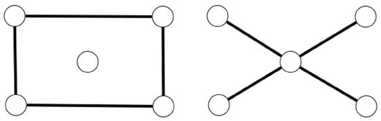
The star graph and a graph formed by the disjoint union of a length-4 cycle and an isolated vertex, , have the same A-spectrum . They are, however, not isomorphic since is connected and is disconnected (see Figure 1).
Figure 1.
The graphs and (i.e., a union of a 4-length cycle and an isolated vertex) are cospectral and nonisomorphic graphs (A-NICS graphs) on five vertices. These two graphs, therefore, cannot be determined by their adjacency matrix.
It can be verified computationally that all the connected nonisomorphic graphs on five vertices can be distinguished by their A-spectrum (see [4] (Appendix A1)).
Theorem 12
([12]). All the regular graphs with fewer than ten vertices are DS (and, as will be clarified later, also -DS for every ).
Example 3
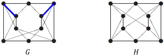
([12]). The two regular graphs in Figure 2 are -NICS.
Figure 2.
-NICS regular graphs on 10 vertices. These cospectral graphs are nonisomorphic because each of the blue edges in belongs to three triangles, whereas no such an edge exists in .
The regular graphs and in Figure 2 can be verified to be cospectral with the common characteristic polynomial
These graphs are also nonisomorphic because each of the two blue edges in belongs to three triangles, whereas no such an edge exists in . Furthermore, it is shown in Example 4.18 of [41] that each pair of the regular NICS graphs on 10 vertices, denoted by and , exhibits distinct values of the Lovász ϑ-functions, whereas the graphs , , , and share identical independence numbers (3), clique numbers (3), and chromatic numbers (4). Furthermore, based on these two pairs of graphs, it is constructively shown in Theorem 4.19 of [41] that for every even integer , there exist connected, irregular, cospectral, and nonisomorphic graphs on n vertices, being jointly cospectral with respect to their adjacency, Laplacian, signless Laplacian, and normalized Laplacian matrices, while also sharing identical independence, clique, and chromatic numbers, but being distinguished by their Lovász ϑ-functions.
Remark 8.
In continuation to Example 3, it is worth noting that closed-form expressions for the Lovász ϑ-functions of regular graphs, which are edge-transitive or strongly regular, were derived in [50] (Theorem 9) and [59] (Proposition 1), respectively. In particular, it follows from [59] (Proposition 1) that strongly regular graphs with identical four parameters are cospectral and they have identical Lovász ϑ-numbers, although they need not be necessarily isomorphic. For such an explicit counterexample, the reader is referred to [59] (Remark 3).
We next introduce friendship graphs to address their possible determination by their spectra with respect to several associated matrices.
Definition 20.
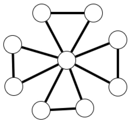
Let . The friendship graph , also known as the windmill graph, is a graph with vertices, consisting of a single vertex (the central vertex) that is adjacent to all the other vertices. Furthermore, every pair of these vertices shares exactly one common neighbor, namely the central vertex (see Figure 3). This graph has edges and p triangles.
Figure 3.
The friendship (windmill) graph has 9 vertices, 12 edges, and 4 triangles.
The term friendship graph in Definition 20 originates from the Friendship Theorem [60]. This theorem states that if is a finite graph where any two vertices share exactly one common neighbor, then there exists a vertex that is adjacent to all other vertices. In this context, the adjacency of vertices in the graph can be interpreted socially as a representation of friendship between the individuals represented by the vertices (assuming friendship is a mutual relationship). For a nice exposition of the proof of the Friendship Theorem, the interested reader is referred to Chapter 44 of [61].
Theorem 13.
The following graphs are DS:
- 1.
- All graphs with fewer than five vertices, and also all regular graphs with fewer than 10 vertices [12] (recall Theorems 11 and 12).
- 2.
- The graphs , , , , and [12].
- 3.
- The complement of the path graph [62].
- 4.
- The disjoint union of k path graph with no isolated vertices, the disjoint union of k complete graphs with no isolated vertices, and the disjoint union of k cycles (i.e., every 2-regular graph) [12].
- 5.
- The complement graph of a DS regular graph [4].
- 6.
- Every -regular graph on n vertices [4].
- 7.
- The friendship graph for [63].
- 8.
- Sandglass graphs, which are obtained by appending a triangle to each of the pendant (i.e., degree-1) vertices of a path [64].
- 9.
- If is a subgraph of a graph , and denotes the graph obtained from by deleting the edges of , then, in addition, the following graphs are DS [21]:
- and , where ;
- ;
- , where has at most four edges.
3.2. Graphs Determined by Their Spectra with Respect to Various Matrices (X-DS Graphs)
In this section, we consider graphs that are determined by the spectra of various associated matrices beyond the adjacency matrix spectrum.
Definition 21.
Let be two graphs and let .
- 1.
- and are said to be -cospectral if they have the same X-spectrum, i.e., .
- 2.
- Nonisomorphic graphs and that are -cospectral are said to be -NICS, where NICS is an abbreviation of nonisomorphic and cospectral.
- 3.
- A graph is said to be determined by its -spectrum (-DS) if every graph that is -cospectral to is also isomorphic to .
Notation 2.
For a singleton , we abbreviate -cospectral, -DS, and -NICS by X-cospectral, X-DS, and X-NICS, respectively. For the adjacency matrix, we will abbreviate A-DS by DS.
Remark 9.
Let . The following holds by definition:
- If two graph are -cospectral, then they are -cospectral.
- If a graph is -DS, then it is -DS.
Definition 22.
Let be a graph. The generalized spectrum of is the -spectrum of .
The following result on the cospectrality of regular graphs can be readily verified.
Proposition 3.
Let and be regular graphs that are -cospectral for some . Then, and are -cospectral for every . In particular, the cospectrality of regular graphs (and their complements) stays unaffected by the chosen matrix among .
Definition 23.
A graph is said to be determined by its generalized spectrum (DGS) if it is uniquely determined by its generalized spectrum. In other words, a graph is DGS if and only if every graph with the same -spectrum as is necessarily isomorphic to .
If a graph is not DS, it may still be DGS, as additional spectral information is available. Conversely, every DS graph is also DGS. For further insights into DGS graphs, including various characterizations, conjectures, and studies, we refer the reader to [65,66,67].
The continuation of this section characterizes graphs that are X-DS, where , with pointers to various studies. We first consider regular DS graphs.
Theorem 14
([12] (Proposition 3)). For regular graphs, the properties of being DS, L-DS, and Q-DS are equivalent.
Remark 10.
To avoid any potential confusion, it is important to emphasize that in statements such as Theorem 14, the only available information is the spectrum of the graph. There is no indication or prior knowledge that the spectrum corresponds to a regular graph. In such cases, the regularity of the graph is not part of the revealed information and, therefore, cannot be used to determine the graph. This recurring approach, which states that is to be a graph that satisfies certain properties (e.g., regularity, strong regularity, etc.) and then examines whether the graph can be determined from its spectrum, appears throughout this paper. It should be understood that the only available information is the spectrum of the graph, and no additional properties of the graph beyond its spectrum are disclosed.
Remark 11.
The crux of the proof of Theorem 14 is that there are no two NICS graphs, with respect to either A, L, or Q, where one graph is regular, and the other is irregular (see [12] (Proposition 2.2)). This, however, does not extend to NICS graphs with respect to the normalized Laplacian matrix , and regular DS graphs are not necessarily -DS. For instance, the cycle and the bipartite complete graph (i.e., ) share the same -spectrum, which is given by , but these graphs are nonisomorphic (as is regular, in contrast to ). It therefore follows that the 2-regular graph is not -DS, although it is DS (see Item 2 of Theorem 13). More generally, it is conjectured in [19] that is -DS if and only if and .
Theorem 15.
The following graphs are L-DS:
- 1.
- and their complements [12].
- 2.
- The disjoint union of k paths, each having at least one edge [12].
- 3.
- The complete bipartite graph with and [68].
- 4.
- The star graphs with [36,39].
- 5.
- Trees with a single vertex having a degree greater than 2 (referred to as starlike trees) [36,39].
- 6.
- The friendship graph [36].
- 7.
- The path-friendship graphs, where a friendship graph and a starlike tree are joined by merging their vertices of degree greater than 2 [38].
- 8.
- The wheel graph for (otherwise, if , then it is not L-DS) [43].
- 9.
- The join of a clique and an independent set on n vertices, , where [69].
- 10.
- Sandglass graphs (see also Item 8 in Theorem 13) [64].
- 11.
- The join graph , for every , where is a disconnected graph [45].
- 12.
- The join graph , for every , where is an L-DS connected graph on n vertices and m edges with , is a connected graph, and either one of the following conditions holds [45]:
- is L-DS;
- the maximum degree of is smaller than .
- 13.
- Specifically, the join graph , for every , where is an L-DS tree on vertices (since, the equality holds for a tree on n vertices and m edges) [45].
Remark 12.
In general, a disjoint union of complete graphs is not determined by its Laplacian spectrum.
Theorem 16.
The following graphs are Q-DS:
- 1.
- The disjoint union of k paths, each having at least one edge [12].
- 2.
- The star graphs with [16,40].
- 3.
- Trees with a single vertex having a degree greater than 2 [16,40].
- 4.
- The friendship graph [70].
- 5.
- The lollipop graphs, where a lollipop graph, denoted by where and , is obtained by appending a cycle to a pendant vertex of a path [26,44].
- 6.
- where is a either a 1-regular graph, an -regular graph of order n or a 2-regular graph with at least 11 vertices [15].
- 7.
- If and , then [42].
- 8.
- If and , then is Q-DS if and only if [42].
- 9.
- The join of a clique and an independent set on n vertices, , where and [69].
Since the regular graphs , , and are DS, they are also -DS for every (see Theorem 14). This, however, does not apply to regular -DS graphs (see Remark 11), which are next addressed.
Theorem 17.
The following graphs are -DS:
- , for every [20].
- The friendship graph , for [14] (Corollary 1).
- More generally, if , or and [14] (Theorem 1).
4. Special Families of Graphs
This section introduces special families of structured graphs, and it states the conditions for their unique determination by their spectra.
4.1. Stars and Graphs of Pyramids
Definition 24.
For every with , define the graph . For , the graph represents the star graph . For , it represents a graph comprising triangles sharing a common edge, which is referred to as a crown. For satisfying , the graphs are referred to as graphs of pyramids [31].
Theorem 18
([31]). The graphs of pyramids are DS for every .
Theorem 19
([31]). The star graph is DS if and only if is prime.
To prove these theorems, a closed-form expression for the spectrum of is derived in [31], which also presents a generalized result. Subsequently, using Theorem 3, the number of edges and triangles in any graph cospectral with are calculated. Finally, Schur’s theorem (Theorem 1) and Cauchy’s interlacing theorem (Theorem 2) are applied in [31] to prove Theorems 18 and 19.
4.2. Complete Bipartite Graphs
By Theorem 19, the star graph is DS if and only if is prime. By Theorem 13, the regular complete bipartite graph is DS for every . Here, we generalize these results and provide a characterization for the DS property of for every .
Theorem 20
([12]). The spectrum of the complete bipartite graph is .
This theorem can be proved by Theorem 1. An alternative simple proof is next presented.
Proof.
The adjacency matrix of is given by
The rank of is equal to 2, so the multiplicity of 0 as an eigenvalue is . By Corollary 3, the two remaining eigenvalues are given by for some since the eigenvalues sum to zero. Furthermore,
so . □
For , the arithmetic and geometric means of are, respectively, given by and . The AM-GM inequality states that for every , we have with equality if and only if .
Definition 25.
Let . The two-element multiset is said to be an AM-minimizer if it attains the minimum arithmetic mean for their given geometric mean, i.e.,
Example 4.
The following are AM-minimizers:
- for every . By the AM-GM inequality, it is the only case where .
- where are prime numbers. In this case, the following family of multisetsonly contains the two multisets , and since .
- where q is a prime number.
Theorem 21.
The following holds for every :
- 1.
- Let be a graph that is cospectral with . Then, up to isomorphism, (i.e., is a disjoint union of the two graphs and ), where is an empty graph and satisfy .
- 2.
- The complete bipartite graph is DS if and only if is an AM-minimizer.
Remark 13.
Item 2 of Theorem 21 is equivalent to Corollary 3.1 of [37], for which an alternative proof is presented here.
Proof. (Proof of Theorem 21):
- 1.
- Let be a graph cospectral with . The number of edges in equals the number of edges in , which is . As is bipartite, so is . Since is of rank 2, and has rank 3, it follows from the Cauchy’s Interlacing Theorem (Theorem 2) that is not an induced subgraph of .It is claimed that has a single nonempty connected component. Suppose to the contrary that has (at least) two nonempty connected components . For , since is a nonempty graph, has at least one eigenvalue . Since is a simple graph, the sum of the eigenvalues of is , so has at least one positive eigenvalue. Thus, the induced subgraph has at least two positive eigenvalues while has only one positive eigenvalue, which contradicts Cauchy’s Interlacing Theorem.Hence, can be decomposed as where is an empty graph. Since and have the same number of edges, , so .
- 2.
- First, we will show that if is not an AM-minimizer, then the graph is not A-DS. This is performed by finding a nonisomorphic graph to that is A-cospectral with it. By assumption, since is not an AM-minimizer, there exist satisfying and . Define the graph where . Observe that . The A-spectrum of both of these graphs is given byso these two graphs are nonisomorphic and cospectral, which means that is not A-DS.We next prove that if is an AM-minimizer, then is A-DS. Let be a graph that is cospectral with . From the first part of this theorem, where and is an empty graph. Consequently, it follows that . Since is assumed to be an AM-minimizer, it follows that , and thus equality holds. Both equalities and can be satisfied simultaneously if and only if , so and .
□
Corollary 6.
Almost all of the complete bipartite graphs are not DS. More specifically, for every , there exists a single complete bipartite graph on n vertices that is DS.
Proof.
Let . By the fundamental theorem of arithmetic, there is a unique decomposition where and are prime numbers for every . Consider the family of multisets
This family has members since every prime factor of n should be in the prime decomposition of a or b. Since the minimization of under the equality constraint forms a convex optimization problem, only one of the multisets in the family is an AM-minimizer. Thus, if , then the number of complete bipartite graphs of n vertices is , and (by Item 2 of Theorem 21) only one of them is DS. □
4.3. Turán Graphs
The Turán graphs are a significant and well-studied class of graphs in extremal graph theory, and they form an important family of multipartite complete graphs. Turán graphs are particularly known for their role in Turán’s theorem, which provides a solution to the problem of finding the maximum number of edges in a graph that does not contain a complete subgraph of a given order [71]. Before delving into formal definitions, it is noted that the distinction of the Turán graphs as multipartite complete graphs is that they are as balanced as possible, ensuring their vertex sets are divided into parts of nearly equal size.
Definition 26.
Let be natural numbers. Define the complete k-partite graph
A graph is multipartite if it is k-partite for some .
Definition 27.
Let . The Turán graph (not to be confused with the graph of pyramids ) is formed by partitioning a set of n vertices into k subsets, with sizes as equal as possible, and then every two vertices are adjacent in that graph if and only if they belong to different subsets. It is, therefore, expressed as the complete k-partite graph , where for all with . Let q and s be the quotient and remainder, respectively, of dividing n by k (i.e., , ), and let . Then,
By construction, the graph has a clique of order k (any subset of vertices with a single representative from each of the k subsets is a clique of order k), but it cannot have a clique of order (since vertices from the same subset are nonadjacent). Note also that, by (42), the Turán graph is a q-regular graph if and only if n is divisible by k, and then .
Definition 28.
Let . Define the regular complete multipartite graph, , to be the k-partite graph with q vertices in each part. Observe that .
Let be a simple graph on n vertices that does not contain a clique of order greater than a fixed number . Turán investigated a fundamental problem in extremal graph theory of determining the maximum number of edges that can have [71].
Theorem 22
(Turán’s Graph Theorem). Let be a graph on n vertices with a clique of order at most k for some . Then,
For a nice exposition of five different proofs of Turán’s Graph Theorem, the interested reader is referred to Chapter 41 of [61].
Corollary 7.
Let , and let be a graph on n vertices where and . Let be a graph obtained by adding an arbitrary edge to . Then, .
4.3.1. The Spectrum of the Turán Graph
Theorem 23
([72]). Let , and let be natural numbers. Let be a complete multipartite graph on vertices. Then,
- has one positive eigenvalue, i.e., and .
- has 0 as an eigenvalue with multiplicity .
- has negative eigenvalues, and
Corollary 8.
The spectrum of the regular complete k-partite graph is given by
Proof.
This readily follows from Theorem 23 by setting . □
Lemma 1
([73]). Let be -regular graphs on vertices for , with the adjacency spectrum and . The A-spectrum of is given by
Theorem 24.
Let such that and The following holds with respect to the A-spectrum of :
- 1.
- If , then the A-spectrum of the irregular Turán graph is given by
- 2.
- If , then , and the A-spectrum of the regular Turán graph is given by
Proof.
Let . We next derive the A-spectrum of an irregular Turán graph in Item 1 of this theorem (i.e., its spectrum if n is not divisible by k since ). By Corollary 8, the spectra of the regular graphs and is
The -partite graph is -regular with , the s-partite graph is -regular with , and by Definition 27, we have . Hence, by Lemma 1, the adjacency spectrum of is given by
where
where the last equality holds since, by the equality and the above expressions of and , it can be readily verified that and . Finally, combining (52)–(55) gives the A-spectrum in (48) of an irregular Turán graph .
We next prove Item 2 of this theorem, referring to a regular Turán graph (i.e., or, equivalently, ). In that case, we have where , so the A-spectrum in (49) holds by Corollary 8. □
Remark 14.
In light of Theorem 24, if , then the number of negative eigenvalues (including multiplicities) of the adjacency matrix of the Turán graph is if the graph is regular (i.e., if ), and it is otherwise (i.e., if the graph is irregular). If , which corresponds to an empty graph (having no edges), then all eigenvalues are zeros (having no negative eigenvalues). Furthermore, the adjacency matrix of always has a single positive eigenvalue, which is of multiplicity 1 irrespectively of the values of n and k. We rely on these properties later in this paper (see Section 4.3.2).
Example 5.
By Theorem 24, let us calculate the A-spectrum of the Turán graph , and verify it numerically with the SageMath software [74]. Having and gives and , which by Theorem 24 implies that
That has been numerically verified by programming in the SageMath software.
4.3.2. Turán Graphs Are DS
The main result of this subsection establishes that all Turán graphs are determined by their A-spectrum. This result is equivalent to Theorem 3.3 in [37], while it also presents an alternative proof that offers additional insights.
Theorem 25.
The Turán graph is A-DS.
In order to prove Theorem 25, we first introduce an auxiliary result from [75], followed by several other lemmata.
Theorem 26
([75] (Theorem 1)). Let be a graph. Then, the following statements are equivalent:
- has exactly one positive eigenvalue.
- for some m, where is a nonempty complete multipartite graph. In other words, the non-isolated vertices of form a complete multipartite graph.
Proof of Theorem 25.
Let be a graph that is A-cospectral with . Denote for such that .
Lemma 2.
The graph does not have a clique of order .
Proof.
Suppose to the contrary that the graph has a clique of order , which means that is an induced subgraph of . The complete graph has k negative eigenvalues ( with a multiplicity of k). On the other hand, has at most negative eigenvalues, zero eigenvalues, and exactly one positive eigenvalue; indeed, this follows from Theorem 24 (see Remark 14), and since and are A-cospectral graphs. Hence, by Cauchy’s Interlacing Theorem, every induced subgraph of on vertices has at most negative eigenvalues (i.e., those eigenvalues interlaced between the negative and zero eigenvalues of that are placed at distance apart in a sorted list of the eigenvalues of in decreasing order). This contradicts our assumption of the existence of a clique of vertices because of the k negative eigenvalues of . □
Lemma 3.
The graph is a complete multipartite graph.
Proof.
Since has exactly one positive eigenvalue, which is of multiplicity one, we obtain from Theorem 26 that for some , where is a nonempty multipartite graph. We next show that . Suppose to the contrary that , and let v be an isolated vertex of . Since is a nonempty graph, there exists a vertex . Let be the graph obtained from by adding the single edge . By Lemma 2, does not have a clique of order . Hence, does not have a clique of order either, contradicting Corollary 7. Hence, . □
Lemma 4.
The graph is a complete k-partite graph.
Proof.
By Lemma 3, is a complete multipartite graph. Let r be the number of partite subsets in the vertex set . We show that , which then gives that is a complete k-partite graph. By Lemma 2, does not have a clique of order . Hence, . Suppose to the contrary that . Since is a complete r-partite graph, the largest order of a clique in is r. Let be a graph obtained from by adding an edge between two vertices within the same partite subset. The graph becomes an -partite graph. Consequently, the maximum order of a clique in is at most . The graph has exactly one more edge than . Since is A-cospectral to , it has the same number of edges as in . Hence, contains more edges than , while also lacking a clique of order . This contradicts Corollary 7, so we conclude that . □
Let be the number of vertices in each partite subset of the complete k-partite graph , i.e., . Then, the next two lemmata subsequently hold.
Lemma 5.
For all , .
Proof.
Suppose to the contrary that there exists a partite subset in the complete k-partite graph with more than vertices. Let be such a partite subset, and suppose without loss of generality that . By the pigeonhole principle, there exists a partite subset of with at most q vertices (since , where ). Let be such a partite subset of , and suppose without loss of generality that . Let be the graph obtained from by removing a vertex , adding a new vertex u to , and connecting u to all the vertices outside its partite subset. The new graph is also k-partite, so it does not contain a clique of order greater than k. Furthermore, by construction, has more edges than , so
Hence, is a graph with no clique of order greater than k, and it has more edges than . That contradicts Theorem 22, so cannot include any element that is larger than . □
Lemma 6.
For all , .
Proof.
The proof of this lemma is analogous to the proof of Lemma 5. Suppose to the contrary that there exists a partite subset of with less than q vertices. Let be such a partite subset, so . By the pigeonhole principle, there exists a partition with at least vertices. Let be such a partite subset set, and let its number of vertices be denoted by . Let be the graph obtained by removing a vertex , adding a new vertex u to , and connecting the vertex u to all the vertices outside its partite subset. is k-partite, so it does not contain a clique of order greater than k, and has more edges than so (57) holds. Hence, is a graph with no clique of order greater than k, and it has more edges than . That contradicts Theorem 22, so cannot include any element that is smaller than q. □
By Lemmas 5 and 6, we conclude that for every . Let be the number of partite subsets of q vertices and be the number of partite subsets of vertices. Since has n vertices, where , it follows that . Moreover, is k-partite, so it follows that . This gives the linear system of equations
which has the single solution
Hence, , which completes the proof of Theorem 25. □
Remark 15.
The proof of Theorem 25 is an alternative proof of Theorem 3.3 in [37]. While both proofs rely on Theorem 26, which is Theorem 1 of [75], our proof relies on the adjacency spectral characterization in Theorem 24, noteworthy in its own right, and further builds upon a sequence of results presented in Lemmata 2–6. On the other hand, the proof of Theorem 3.3 in [37] relies on Theorem 26, but then deviates substantially from our proof (see Lemmata 2.4 and 2.5 in [37] and Theorem 3.1 in [37] and serves to prove Theorem 25).
4.4. Line Graphs
Among the various studied transformations on graphs, the line graphs of graphs are one of the most studied transformations [76]. We first introduce their definition, and then address the spectral graph determination properties.
Definition 29.
The line graph of a graph , denoted by , is a graph whose vertices are the edges in , and two vertices are adjacent in if the corresponding edges are incident in .
A notable spectral property of line graphs is that all the eigenvalues of their adjacency matrix are greater than or equal to (see, e.g., [76] (Theorem 4.6)). For the determination of all graphs whose spectrum is bounded from below by , the interested reader is referred to [76] (Section 4.5).
The following theorem characterizes some families of line graphs that are DS.
Theorem 27.
The following line graphs are DS:
- 1.
- The line graph of the complete graph , where and (see [4] (Theorem 4.1.7));
- 2.
- The line graph of the complete bipartite graph , where and (see [4] (Theorem 4.1.8));
- 3.
- The line graph (see [4] (Proposition 4.1.5));
- 4.
- The line graph of the complete bipartite graph , where and with (see [4] (Proposition 4.1.18)).
Remark 16.
In regard to Item 1 of Theorem 27, the line graphs of complete graphs are referred to as triangular graphs. These are strongly regular graphs with the parameters , where . For , the corresponding triangular graph is cospectral and nonisomorphic to the three Chang graphs (see Remark 4), which are strongly regular graphs .
We next prove the following result in regard to the Petersen graph, which appears in [4] (Problem 4.3) and [51] (Section 10.3) (without a proof).
Corollary 9.
The Petersen graph is DS.
Proof.
The Petersen graph is known to be isomorphic to the complement of the line graph of the complete graph (i.e., it is isomorphic to . By Item 1 of Theorem 27, the line graph is DS. It is also a 6-regular graph (as the line graph of a d-regular graph is -regular and is a 4-regular graph). Consequently, by Item 5 of Theorem 13, the complement of is also DS. □
The following definition and theorem provide further elaboration on Item 2 of Theorem 27.
Definition 30
([51] (Section 1.1.8)). The Hamming graph , where , has the vertex set , and any two vertices are adjacent if and only if they differ in one coordinate (i.e., their Hamming distance is equal to 1). These are also referred to lattice graphs, and denoted by . The Lattice graph , where , is also the line graph of the complete bipartite graph , and it is a strongly regular graph with parameters .
Theorem 28
([77]). The lattice graph is a strongly regular DS graph for all . For , the graph is not DS since it is cospectral and nonisomorphic to the Shrikhande graph, which are nonisomorphic strongly regular graphs with the common parameters .
The following result provides an interesting connection between A and Q-cospectralities of graphs.
Theorem 29
([4] (Proposition 7.8.5)). If two graphs are Q-cospectral, then their line graphs are A-cospectral.
4.5. Nice Graphs
The family referred to as “nice graphs” has been recently introduced in [9].
Definition 31.
- A graph is sunlike if it is connected and can be obtained from a cycle by adding some vertices and connecting each of them to some vertex in .
- Let . A sunlike graph is-nice if it can be obtained by a cycle and
- -
- There is a single vertex of degree 3.
- -
- There are k vertices of degree 4. Let .
- -
- By starting a walk on from at some orientation, then after 4 or 6 steps, we get to a vertex . Then, after another 4 or 6 steps from we get to , and so on, until we get to the vertex .
Theorem 30
([9]). Let such that . Let be an -nice graph. If the order of is a prime number greater than some , then the line graph is DS.
A more general class of graphs is introduced in [9], where it is shown that for every sufficiently large , the number of nonisomorphic n-vertex DS graphs is at least for some positive constant c (see [9] (Theorem 1.4)). This recent result represents a significant advancement in the study of Haemers’ conjecture because the earlier lower bounds on the number of nonisomorphic n-vertex DS graphs were all of the form , for some positive constant c. As noted in [9], the first form of such a lower bound was derived by van Dam and Haemers [13] (Proposition 6), who proved that a graph is DS if every connected component of is a complete subgraph, leading to a lower bound that is approximately of the form with . Therefore, the transition to a lower bound in [9] that scales exponentially with n, rather than with , is both remarkable and noteworthy.
4.6. Friendship Graphs and Their Generalization
The next theorem considers whether friendship graphs (see Definition 20) can be uniquely determined by the spectra of four of their associated matrices.
Theorem 31.
The friendship graph satisfies the following properties: It is DS if and only if (i.e., the friendship graph is DS unless it has 16 triangles) [63], L-DS [78], Q-DS [70], and -DS [14].
The friendship graph , where , can be expressed in the form (see Figure 3). The last observation follows from a property of a generalized friendship graph, which is defined as follows.
Definition 32.
Let . The generalized friendship graph is given by . Note that .
The following theorem addresses the conditions under which generalized friendship graphs can be uniquely determined by the spectra of their normalized Laplacian matrix.
Theorem 32.
The generalized friendship graph is -DS if and only if or both and [14].
Corollary 10.
The friendship graph is -DS [14].
4.7. Strongly Regular Graphs
Strongly regular graphs with an identical vector of parameters are cospectral but may not be isomorphic (see, Corollary 4, Remark 4, and Theorem 28). For that reason, strongly regular graphs are not necessarily determined by their spectrum. There are, however, infinite families of strongly regular DS graphs:
Theorem 33
([1] (Proposition 14.5.1)). If , , , and , then the disjoint union of identical complete graphs , the line graph of a complete graph , and the line graph of a complete bipartite graph with partite sets of equal size , as well as their complements, are strongly regular DS graphs.
We next show that, although connected strongly regular graphs are not generally DS, the property of strong regularity, as well as the four parameters that characterize strongly regular graphs can be determined by the spectrum of their adjacency matrix.
Theorem 34.
Let be a connected strongly regular graph. Then, its strong regularity, the vector of parameters , Lovász ϑ-function , number of edges and triangles, girth, and diameter can all be determined by its A-spectrum.
Proof.
The order of a graph n is determined by the A-spectrum, which is the number of eigenvalues (including multiplicities). By Theorem 4, the regularity of a graph is determined by its A-spectrum. By Item 5 of Theorem 5, a connected regular graph is strongly regular if and only if it has three distinct eigenvalues. Hence, the strong regularity property of is determined by its A-spectrum. For such a connected regular, the largest eigenvalue is simple, , and the other two distinct eigenvalues of the adjacency matrix of are given by and with . We next show that the number of common neighbors of any pair of adjacent vertices (), and the number of common neighbors of any pair of nonadjacent vertices () in are, respectively, given by
So, these parameters are explicitly expressed in terms of the adjacency spectrum of the strongly regular graph. Indeed, by Theorem 5, the second-largest and least eigenvalues of the adjacency matrix of are given by
from which it follows that (noting that )
This gives (60) and (61) from, respectively, the second equality in (63) and by adding the two equalities in (63).
The Lovász -function of a strongly regular graph is given by (see [59] (Proposition 1))
so is determined by its A-spectrum since the strong regularity property of was first determined. The number of edges of a d-regular graph is given by , and the number of triangles of the strongly regular graph is given by , so they are both determined once the four parameters of the strongly regular graphs are revealed. The diameter of a connected strongly regular graph is equal to 2 (note that complete graphs are excluded from the family of strongly regular graphs). Finally, the girth of the strongly regular graph is determined as follows [79]:
- 1.
- If , then the girth of is equal to 3;
- 2.
- If and , then the girth of is equal to 4;
- 3.
- If and , then the girth of is equal to 5.
□
Remark 17.
A strongly regular graph is connected if and only if .
By [12] (Proposition 2), no pair of A-cospectral graphs exists where one graph is regular and the other is not. The following result extends this observation to strong regularity.
Corollary 11.
There are no two A-cospectral connected graphs where one is strongly regular and the other is not.
Proof.
For a connected strongly regular graph, the strong regularity is determined by the A-spectrum. □
Another corollary that follows from Theorem 34 applies to strongly regular DS graphs.
Corollary 12.
Let be a connected strongly regular graph such that there is no other nonisomorphic strongly regular graph with an identical vector of parameters . Then, is a DS graph.
Corollary 12 naturally raises the following question.
Question 1.
Which connected strongly regular graphs are determined by their vector of parameters ?
A partial answer to Question 1 is provided below.
By Corollary 12, for connected strongly regular graphs, there exists an equivalence between their spectral determination (due to their regularity and in light of Theorem 14, which is based on the spectrum of their adjacency, Laplacian, or signless Laplacian matrices) and the uniqueness of these graphs for the given parameter vector .
The study of the number of nonisomorphic strongly regular graphs corresponding to a given set of parameters has been extensively explored. For example, by Theorem 28, there is a unique (up to isomorphism) strongly regular graph of the form for any given with . Specifically, this implies the uniqueness of (setting ). On the other hand, a computer search by McKay and Spence established that there are 32,548 strongly regular graphs of the form , so none of them is DS (by Corollary 12).
Further results on the uniqueness or non-uniqueness of strongly regular graphs with a given parameter vector can be found in [80] and the references therein. Infinite families of strongly regular DS graphs are presented in Theorem 33. Some known sporadic, strongly regular DS graphs are listed in [12] (Table 2), with an update in [13] (Table 1). The uniqueness of further strongly regular graphs with given parameter vectors, which makes them, therefore, DS graphs, was established, e.g., in [81,82,83,84,85].
A combination of [13] (Table 1) and Corollary 9 implies that, apart from complete graphs on fewer than three vertices and all complete bipartite regular graphs (which are known to be DS, as stated in Item 2 of Theorem 13), also all the seven currently known triangle-free strongly regular graphs (see [86]) are DS. These include the following:
- The Pentagon graph that is (by Item 2 of Theorem 13, and see [51] (Section 10.1));
- The Petersen graph (by Corollary 9, and see [51] (Section 10.3));
- Clebsch graph (see [51] (Section 10.7));
- Hoffman–Singleton srg (see [51] (Section 10.19));
- Gewirtz graph (see [51] (Section 10.20));
- Mesner () graph (see [51] (Section 10.27) and [81]);
- Higman–Sims graph (see [51] (Section 10.31) and [85]).
An up-to-date list of strongly regular DS graphs—strongly regular graphs that are uniquely determined by their parameter vectors—as well as the number of strongly regular NICS graphs for given parameter vectors, is available on Brouwer’s website [87]. An exclamation mark placed to the left of a parameter vector , when it is without a preceding number, indicates a strongly regular DS graph. In contrast, an exclamation mark preceded by a natural number greater than 1 specifies the number of strongly regular NICS graphs with the corresponding parameter vector. For example, as shown in [87], strongly regular graphs with the parameter vectors , , , and , among others, are DS graphs. On the other hand, according to [87], there are 15 strongly regular NICS graphs with the parameter vector , 10 strongly regular NICS graphs with the parameter vector , and so forth.
To conclude, as strongly regular NICS graphs are not DS, L-DS, or Q-DS, we were recently informed of ongoing research by Cioaba et al. [88], which investigates the spectral properties of higher-order Laplacian matrices associated with these graphs. This research demonstrates that the spectra of these new matrices can distinguish some of the strongly regular NICS graphs. However, in other cases, strongly regular NICS graphs remain indistinguishable even with the spectra of these higher-order Laplacian matrices.
5. Graph Operations for the Construction of Cospectral Graphs
This section presents such graph operations, focusing on unitary and binary transformations that enable the systematic construction of cospectral graphs. These operations are designed to preserve the spectral properties of the original graph while potentially altering its structure, thereby producing nonisomorphic graphs with identical eigenvalues. By employing these techniques, one can generate diverse examples of cospectral graphs, which offer valuable tools for investigating the limitations of spectral characterization and exploring the boundaries between graphs that are or are not determined by their spectrum, which then relates the scope of the present section to Section 4, which deals with graphs or graph families that are determined by their spectrum.
5.1. Coalescence
A construction of cospectral trees has been offered in [11], implying that almost all trees are not DS.
Definition 33.
Let be two graphs with , vertices, respectively. Let and be an arbitrary choice of vertices in both graphs. The coalescence of and with respect to and is the graph with vertices, obtained by the union of and where and are identified as the same vertex in the united graph.
Theorem 35.
Let be two cospectral graphs, and let and be an arbitrary choice of vertices in both graphs. Let and be the subgraphs of and that are induced by and , respectively. Let Γ be a graph and . If and are cospectral, then the coalescence of and Γ with respect to and u is cospectral to the coalescence of and Γ with respect to and u.
Combinatorial arguments that rely on the coalescence operation on graphs lead to a striking asymptotic result in [11], which states that the fraction of n-vertex trees with cospectral and nonisomorphic mates, which are also trees, approaches one as n tends to infinity. Consequently, the fraction of the n-vertex nonisomorphic trees that are determined by their spectrum (DS) approaches zero as n tends to infinity. In other words, this means that almost all trees are not DS (with respect to their adjacency matrix) [11].
5.2. Seidel Switching
Seidel switching is one of the well-known methods for the construction of cospectral graphs.
Definition 34.
Let be a graph, and let . Constructing a graph by preserving all the edges in between vertices within , as well as all edges in between vertices within the complement set , while modifying adjacency and nonadjacency between any two vertices where one is in and the other is in , is referred to (up to isomorphism) as Seidel switching of with respect to .
By Definition 34, the Seidel switching of with respect to is equivalent to its Seidel switching with respect to . Let and be the adjacency matrices of a graph and its Seidel switching , and let and be the matrices of that, respectively, refer to the adjacency matrices of the subgraphs of induced by and . Then, for some , we obtain
and by Definition 34,
where is obtained from by interchanging zeros and ones. If is a regular graph, the following is a necessary and sufficient condition for to be a regular graph of the same degree of its vertices.
Theorem 36
([4] (Proposition 1.1.7)). Let be a d-regular graph on n vertices. Then, is also d-regular if and only if induces a regular subgraph of degree k, where .
The next result shows the relevance of Seidel switching for the construction of regular and cospectral graphs.
Theorem 37
([4] (Proposition 1.1.8)). Let be a d-regular graph, , and let be obtained from by Seidel switching. If is also a d-regular graph, then and are cospectral (and due to their regularity, they are -cospectral for every ).
Remark 18.
Theorem 37 provides a method for finding cospectral regular graphs. These graphs may be, however, also isomorphic. If the graphs are nonisomorphic, then it gives a pair of NICS graphs.
Remark 19.
A regular graph on n vertices cannot be switched into another regular graph if n is odd (see [4] (Corollary 4.1.10)), which means that the conditions in Theorem 37 cannot be satisfied for any regular graph of an odd order.
Remark 20.
Seidel switching determines an equivalence relation on graphs. This follows from the fact that switching with respect to a subset , and then with respect to a subset , is the same as switching with respect to (see [4] (p. 18)).
Example 6.
The Shrikhande graph can be obtained through Seidel switching applied to the line graph with respect to four independent vertices of the latter (see [4] (Example 1.2.4)). Both are 6-regular graphs (hence, they are cospectral graphs by Theorem 37). Moreover, the former graph is a strongly regular graph , whereas the line graph is not. Consequently, these are nonisomorphic and cospectral (NICS) 6-regular graphs on 16 vertices.
5.3. The Godsil and McKay Method
Another construction of cospectral pairs of graphs was offered by Godsil and McKay in [24].
Theorem 38.
Let be a graph with an adjacency matrix of the form
where the sum of each column in is either or . Let be the matrix obtained by replacing each column in whose sum of elements is with its complement . Then, the modified graph whose adjacency matrix is given by
is cospectral with .
Two examples of pairs of NICS graphs are presented in Section 1.8.3 of [1].
5.4. Graphs Resulting from the Duplication and Corona Graphs
Definition 35
([89]). Let be a graph with a vertex set , and consider a copy of with a vertex set , where is a duplicate of the vertex . For each , connect the vertex to all the neighbors of in , and then delete all edges in . Similarly, for each , connect the vertex to all the neighbors of in the copied graph, and then delete all edges in the copied graph. The resulting graph, which has vertices, is called the duplication graph of , and is denoted by (see Figure 4).
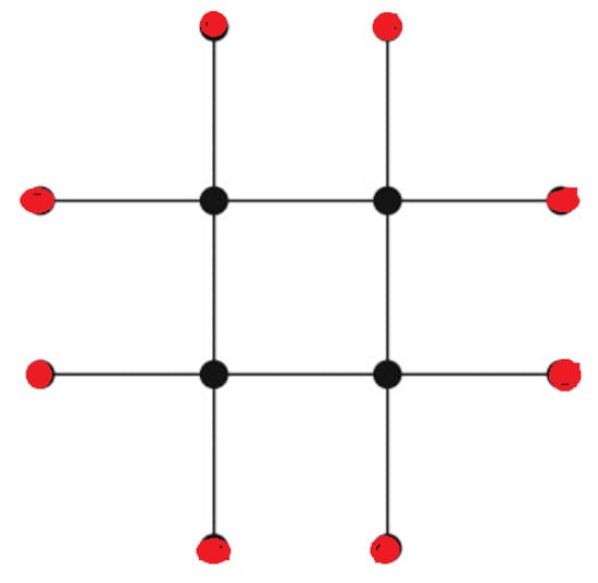
Figure 4.
The duplication graph (see Definition 35).
Definition 36
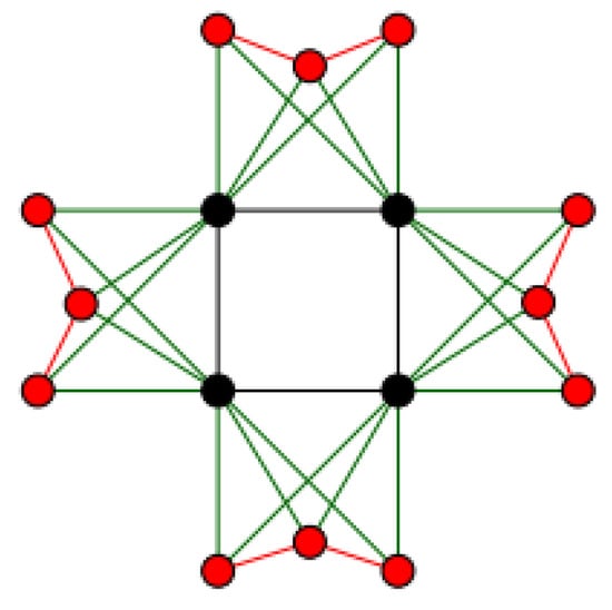
([90]). Let and be graphs on disjoint vertex sets of and vertices, and with and edges, respectively. The corona of and , denoted by , is a graph on vertices obtained by taking one copy of and copies of , and then connecting, for each , the i-th vertex of to each vertex in the i-th copy of (see Figure 5).
Figure 5.
The corona graph (see Definition 36). It is composed of one copy of (referring to the black vertices) and four copies of (referring to the red vertices).
Definition 37
([91]). The edge corona of and , denoted by , is defined as the graph obtained by taking one copy of and copies of , and then connecting, for each , the two end-vertices of the j-th edge of to every vertex in the j-th copy of (see Figure 6).
Figure 6.
The edge-corona graph (see Definition 37).
Definition 38.
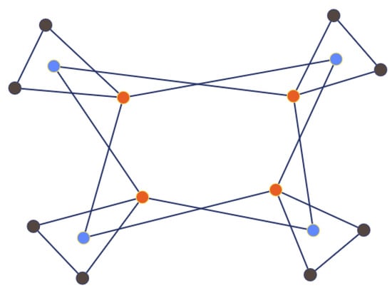
Let and be graphs with disjoint vertex sets of and vertices, respectively. Let be the duplication graph of with vertex set , where and with the duplicated vertex set (see Definition 35). The duplication corona graph, denoted by , is the graph obtained from and copies of by connecting, for each , the vertex of the graph to every vertex in the i-th copy of (see Figure 7).
Figure 7.
The duplication corona graph (see Definition 38).
Definition 39.
Let and be graphs with disjoint vertex sets of and vertices, respectively. Let be the duplication graph of with the vertex set , where and the duplicated vertex set (see Definition 35). The duplication neighborhood corona, denoted by , is the graph obtained from and copies of by connecting the neighbors of the vertex of to every vertex in the i-th copy of for (see Figure 8).
Figure 8.
The duplication neighborhood corona (see Definition 39).
Definition 40.
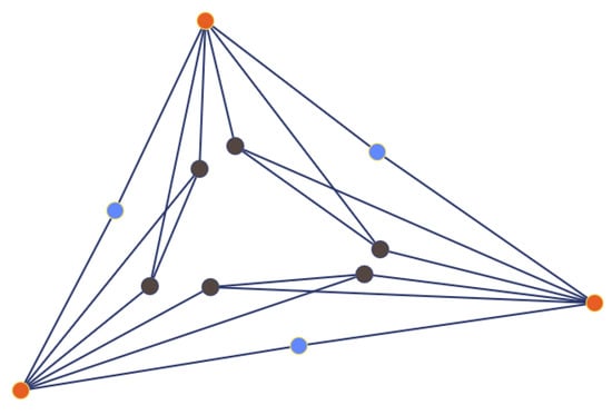
Let and be graphs with disjoint vertex sets of and vertices, respectively. Let be the duplication graph of with vertex set , where is the vertex set of and is the duplicated vertex set. The duplication edge corona, denoted by , is the graph obtained from and copies of by connecting each of the two vertices of to every vertex in the k-th copy of whenever (see Figure 9).
Figure 9.
The duplication edge corona (see Definition 40).
Definition 41.
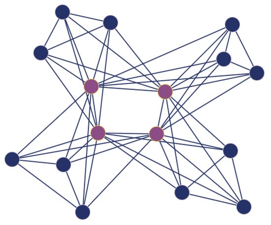
Consider two graphs and with and vertices and, respectively. The closed neighborhood corona of and , denoted by , is a new graph obtained by creating copies of . Each vertex of the copy of is then connected to the vertex and neighborhood of the vertex of (see Figure 10).
Figure 10.
The closed neighborhood corona of the 4-length cycle and the triangle , denoted by (see Definition 41).
Theorem 39
([92]). Let be -regular, cospectral graphs, and let and be -regular, cospectral, and nonisomorphic (NICS) graphs. Then, the following holds:
- The duplication corona graphs and are -NICS irregular graphs.
- The duplication neighborhood corona and are -NICS irregular graphs.
- The duplication edge corona and are -NICS irregular graphs.
Question 2.
Are the irregular graphs in Theorem 39 also cospectral with respect to the normalized Laplacian matrix?
Theorem 40
([93]). Let and be cospectral regular graphs, and let be an arbitrary graph. Then, the following holds:
- The closed neighborhood corona and are -NICS irregular graphs.
- The closed neighborhood corona and are -NICS irregular graphs.
Question 3.
Are the irregular graphs in Theorem 40 also cospectral with respect to the normalized Laplacian matrix?
5.5. Graph Constructions Based on the Subdivision and Bipartite Incidence Graphs
Definition 42
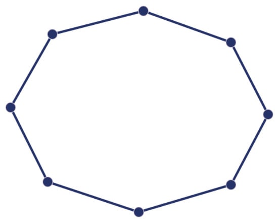
([4]). Let be a graph. The subdivision graph of , denoted by , is obtained from by inserting a new vertex into every edge of . Subdivision is the process of adding a new vertex along an edge, effectively splitting the edge into two edges connected in series through the new vertex (see Figure 11).
Figure 11.
The subdivision graph of a 4-length cycle, denoted by , which is an 8-length cycle (see Definition 42).
Definition 43
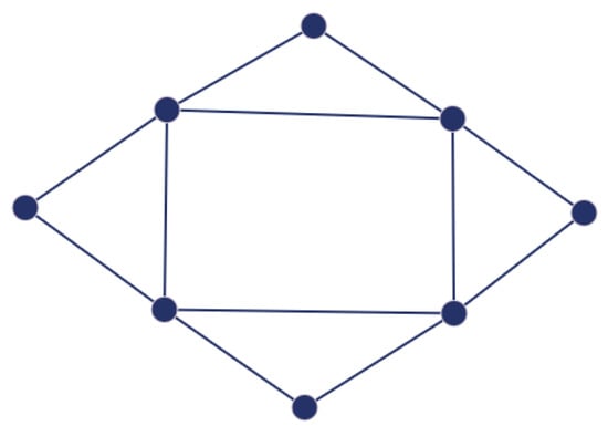
([94]). Let be a graph. The bipartite incidence graph of , denoted by , is a bipartite graph constructed as follows: For each edge , a new vertex is added to the vertex set of . The vertex is then made adjacent to both endpoints of e in (see Figure 12).
Figure 12.
The bipartite incidence graph of a length-4 cycle , denoted by (see Definition 43).
Let and be two vertex-disjoint graphs with and vertices, and and edges, respectively. Four binary operations on these graphs are defined as follows.
Definition 44.
The subdivision-vertex-bipartite-vertex join of graphs and , denoted , is the graph obtained from and by connecting each vertex of (that is the subset of the original vertices in the vertex set of ) with every vertex of (that is the subset of the original vertices in the vertex set of ).
By Definitions 42, 43, and 44, it follows that the graph has vertices and edges. Figure 13 displays the graph .
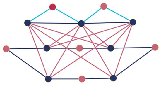
Figure 13.
The graph (see Definition 44). The black vertices represent the vertices of the length-4 cycle and the vertices of the path . The additional vertices in the subdivision graph are the four red vertices located at the bottom of this figure (as shown in Figure 11). Similarly, the additional vertices in the bipartite incidence graph of the path are the two red vertices located at the top of this figure. The edges of the graph include the following: edges connecting each black vertex of to each black vertex of , edges between the black and red vertices at the bottom of the figure (that correspond to the subdivision of ), and the four (light blue) edges connecting the two top red vertices to the top black vertices of the figure (that correspond to the bipartite incidence graph of ).
Definition 45.
The subdivision-edge-bipartite-edge join of and , denoted by , is the graph obtained from and by connecting each vertex of (that is the subset of the added vertices in the vertex set of ) with every vertex of (that is the subset of the added vertices in the vertex set of ).
By Definitions 42, 43, and 45, it follows that the graph has vertices and edges. Figure 14 displays the graph .
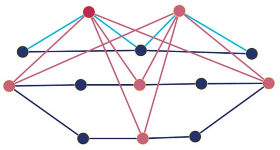
Figure 14.
The graph (see Definition 45). In comparison to Figure 13, edges connecting each black vertex of to each black vertex of are deleted and replaced in this figure by edges connecting each red vertex of to each red vertex of .
Definition 46.
The subdivision-edge-bipartite-vertex join of and , denoted by , is the graph obtained from and by connecting each vertex of (that is the subset of the added vertices in the vertex set of ) with every vertex of (that is the subset of the original vertices in the vertex set of ).
By Definitions 42, 43, and 46, it follows that the graph has vertices and edges. Figure 15 displays the graph .
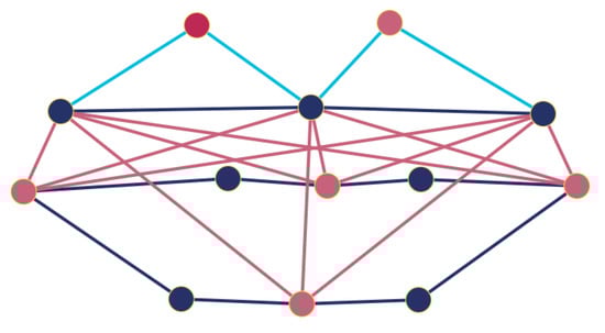
Figure 15.
The graph (see Definition 46). In comparison to Figure 13, edges connecting each black vertex of to each black vertex of are deleted and replaced in this figure by edges connecting each red vertex of to each black vertex of .
Definition 47.
The subdivision-vertex-bipartite-edge join of and , denoted by , is the graph obtained from and by connecting each vertex of (that is the subset of the original vertices in the vertex set of ) with every vertex of (that is the subset of the added vertices in the vertex set of ).
By Definitions 42, 43, and 47, it follows that the graph has vertices and edges. Figure 16 displays the graph .
Figure 16.
The graph (see Definition 47). In comparison to Figure 13, edges connecting each black vertex of to each black vertex of are deleted and replaced in this figure by edges connecting each black vertex of to each red vertex of .
We next present the main result of this subsection, which motivates the four binary graph operations introduced in Definitions 44–47.
Theorem 41
([22]). Let , , where , be regular graphs, where need not be different from . If and are A-cospectral, and and are A-cospectral, then the following holds:
- and are irregular -NICS graphs.
- and are irregular -NICS graphs.
- and are irregular -NICS graphs.
- and are irregular -NICS graphs.
In light of Theorem 41, the following questions naturally arises.
Question 4.
Are the graphs in Theorem 41 also cospectral with respect to the signless Laplacian matrix (i.e., Q-cospectral)?
5.6. Connected Irregular NICS Graphs
The (joint) cospectrality of regular graphs with respect to their adjacency, Laplacian, signless Laplacian, and normalized Laplacian matrices can be asserted by verifying their cospectrality with respect to only one of these matrices. In other words, regular graphs are X-cospectral for some if and only if they are cospectral with respect to all these matrices (see Proposition 3). For irregular graphs, this does not hold in general. Following [17], it is natural to ask the following question:
Question 5.
Are there pairs of irregular graphs that are -NICS, i.e., X-NICS with respect to every ?
This question remained open until two coauthors of this paper recently proposed a method for constructing pairs of irregular graphs that are X-cospectral with respect to every , providing explicit constructions [25]. Building on that work, another coauthor of this paper demonstrated in [41] that for every even integer , there exist two connected, irregular -NICS graphs on n vertices with identical independence, clique, and chromatic numbers, yet distinct Lovász -functions. We now present the preliminary definitions required to outline the relevant results in [25,41], and the construction of such cospectral irregular X-NICS graphs for all .
Definition 48
(Neighbors splitting join of graphs [95]). Let and be graphs with disjoint vertex sets, and let . The neighbors splitting (NS) join of and is obtained by adding vertices to the vertex set of and connecting to if and only if . The NS join of and is denoted by .
Definition 49
(Nonneighbors splitting join of graphs [25,96]). Let and be graphs with disjoint vertex sets, and let . The nonneighbors splitting (NNS) join of and is obtained by adding vertices to the vertex set of and connecting to , with , if and only if . The NNS join of and is denoted by .
Remark 21.
In general, and (unless ).
Example 7
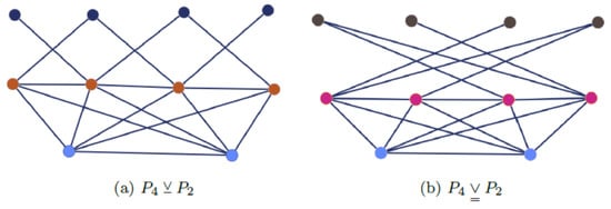
(NS and NNS join of graphs [25]). Figure 17 shows the NS and NNS joins of the path graphs and , denoted by and , respectively.
Figure 17.
The neighbors splitting (NS) and nonneighbors splitting (NNS) joins of the path graphs and are depicted, respectively, on the left and right-hand sides of this figure. The NS and NNS joins of graphs are, respectively, denoted by and [25].
Theorem 42
(Irregular -NICS graphs). Let and be regular and cospectral graphs, and let and be regular, nonisomorphic, and cospectral (NICS) graphs. Then, the following statements hold:
- 1.
- The NS-join graphs and are irregular -NICS graphs.
- 2.
- The NNS join graphs and are irregular -NICS graphs.
The proof of Theorem 42 is provided in [25,96], and it relies heavily on the notion of the Schur complement (see Theorem 1). The interested reader is referred to the recently published paper [25] for further details.
Relying on Theorem 42, the following result is stated and proved in [41].
Theorem 43
(On irregular NICS graphs). For every even integer , there exist two connected, irregular -NICS graphs on n vertices with identical independence, clique, and chromatic numbers, yet their Lovász ϑ-functions are distinct.
That result is, in fact, strengthened in Section 4.2 of [41], and the interested reader is referred to that paper for further details. The proof of Theorem 43 is also constructive, providing explicit such graphs.
6. Open Questions and Outlook
We conclude this paper by highlighting some of the most significant open questions in the fascinating area of research related to cospectral nonisomorphic graphs and graphs determined by their spectrum, leaving them as topics for further future study.
6.1. Haemers’ Conjecture
Haemers’ conjecture [7,8], a prominent topic in spectral graph theory, posits that almost all graphs are uniquely determined by their adjacency spectrum. This conjecture suggests that, for large graphs, the probability of having two nonisomorphic graphs, on a large number of vertices, share the same adjacency spectrum is negligible. The conjecture has inspired extensive research, including studies on specific graph families, cospectrality, and algebraic graph invariants, contributing to deeper insights into the relationship between graph structure and eigenvalues. Haemers’ conjecture is stated formally as follows.
Definition 50.
For , let to be the numbers of distinct graphs on n vertices, up to isomorphism. For , let be the number of -DS graphs on n vertices, up to isomorphism, and (for the sake of simplicity of notation) let
Conjecture 1
([7]). For sufficiently large n, almost all of the graphs are DS, i.e.,
Several results lend support to this conjecture [7,9,10], but a complete proof remains elusive. By [5], the number of graphs with n vertices up to isomorphism is
where . By Stirling’s approximation for and straightforward algebra, can be verified to be given by
It is shown in [9] that the number of DS graphs on n vertices is at least for some constant (see also the discussion in Section 4.5). In light of Remark 9, Conjecture 1 leads to the following question.
Question 6.
For what minimal subset (if any) does the limit
hold?
Some computer results somewhat support Haemers’ Conjecture. Approximately of the graphs with 12 vertices are DS [97]. A new class of graphs is defined in [10], which offers an algorithmic method for finding all the -cospectral mates of a graph in this class (i.e., graphs that are -cospectral with ). Using this algorithm, they found that out of graphs with 50 vertices, which were chosen uniformly at random from this class, at least of them were -DS.
6.2. DS Properties of Structured Graphs
This paper explores various structures of graph families determined by their spectrum with respect to one or more of their associated matrices, as well as the related problem of constructing pairs of nonisomorphic graphs that are cospectral with respect to some or all of these matrices. Several questions are interspersed throughout the paper (see Questions 1, 2, 3, 4, and 5), which remain open for further study.
In addition to serving as a survey on spectral graph determination, this paper suggests a new alternative proof to Theorem 3.3 in [37], asserting that all Turán graphs are determined by their adjacency spectrum (see Theorem 25). This proof is based on a derivation of the adjacency spectrum of the family of Turán graphs (see Theorem 24). Since these graphs are generally bi-regular multipartite graphs (i.e., their vertices have only two possible degrees, which in this case are consecutive integers), it does not necessarily imply that Turán graphs are determined by the spectrum of some other associated matrices, such as the Laplacian, signless Laplacian, or normalized Laplacian matrices. Determining whether this holds is an open question.
The distance matrix of a connected graph is the symmetric matrix whose columns and rows are indexed by the graph vertices, and its entries are equal to the pairwise distances between the corresponding vertices. The distance spectrum is the multiset of eigenvalues of the distance matrix, and its characterization has been a subject of fruitful research (see [98,99] for comprehensive surveys on the distance spectra of graphs, and [100,101] on the spectra of graphs with respect to variants of the distance matrix). Nonisomorphic graphs may share an identical adjacency spectrum, as well as an identical distance spectrum, and, therefore, they are graphs that are not determined by either their adjacency or distance spectrum. This holds, e.g., for the Shrikhande graph and the line graph of the complete bipartite graph , which are nonisomorphic strongly regular graphs with the identical parameters ; they share an identical A-spectrum given by and an identical distance spectrum given by . There exist, however, graphs that are determined by their distance spectrum but are not determined by their adjacency spectrum. In this context, [27] proves that complete multipartite graphs are uniquely determined by their distance spectra (this result confirms a conjecture proposed in [102] and extends the special case established there for complete bipartite graphs). A Turán graph is, in particular, determined by its distance spectrum [27], and by its adjacency spectra (see Theorem 25 here). On the other hand, while complete multipartite graphs are not generally determined by their adjacency spectra (e.g., for complete bipartite graphs, see Theorem 21), they are necessarily determined by their distance spectra [27]. Another family of graphs that are determined by their distance spectrum but are not determined by their adjacency spectrum, named d-cube graphs, is provided in [29,30]. These graphs have their vertices represented by binary n-length tuples, where any two vertices are adjacent if and only if their corresponding binary n-tuples differ in one coordinate; it is also shown that these graphs have exactly three distinct distance eigenvalues. The question of which multipartite graphs, or graphs in general, are determined by their distance spectra remains open.
Another newly obtained proof presented in this paper refers to a necessary and sufficient condition in [37] for complete bipartite graphs to be A-DS (see Theorem 21 and Remark 13 here). These graphs are also bi-regular, and the two possible vertex degrees can differ by more than one. Both of these newly obtained proofs, discussed in Section 4, provide insights into the broader question of which (structured) multipartite graphs are determined by their adjacency spectrum or, more generally, by the spectra of some of their associated matrices.
Even if Haemers’ conjecture is eventually proved in its full generality, it remains surprising when a new family of structured graphs is shown to be DS (or X-DS, more generally). This is because, for certain structured graphs, such as strongly regular graphs and trees, their spectra often fail to uniquely determine them [12,13]. This stark contrast between the fact that almost all random graphs of high order are likely to be DS and the existence of interesting structured graphs that are not DS has significant implications.
In addition to the questions posed earlier in this paper, we raise the following additional concrete question:
Question 7.
By Theorem 32, the family of generalized friendship graphs is -DS. Are these graphs also DS with respect to their other associated matrices?
We speculate that the DS property of a graph correlates, to some extent, with the number of symmetries that the graph possesses, and we hypothesize that the size of the automorphism group of a graph can partially indicate whether it is DS.
A justification for this claim is that the automorphism group of a graph reflects its symmetries, which can influence the eigenvalues of its adjacency matrix. Highly symmetric graphs (i.e., those with large automorphism groups) often exhibit eigenvalue multiplicities and patterns that are shared by other nonisomorphic graphs, making such graphs less likely to be DS. Conversely, graphs with trivial automorphism groups are typically less symmetric and may have eigenvalues that uniquely determine their structure, increasing the likelihood that they are DS. As noted in [5], almost all graphs have trivial automorphism groups. This observation aligns with the conjecture that most graphs are DS, as the absence of symmetry reduces the likelihood of two nonisomorphic graphs sharing the same spectrum.
It is noted, however, that the DS property of graphs is not solely dictated by their automorphism groups. Specifically, a graph with a large automorphism group can still be DS if its eigenvalues uniquely encode its structure (see Section 4.7). In contrast to these DS graphs, other graphs with trivial automorphism groups are not guaranteed to be DS; in such cases, the spectrum might not capture enough structural information to uniquely determine the graph. Typically, graphs with a small number of distinct eigenvalues seem to be, in general, the hardest graphs to distinguish by their spectrum. As noted in [103], it seems that most graphs with few eigenvalues (e.g., most of the strongly regular graphs) are not determined by their spectrum, which served as one of the motivations of the work in [103] in studying graphs whose normalized Laplacian has three eigenvalues.
To conclude, the size of the automorphism group of a graph can provide some indication of whether it is DS, but it is not a definitive criterion. While large automorphism groups often correlate with the graph not being DS due to shared eigenvalues among nonisomorphic graphs, this is not an absolute rule. Therefore, the claim should be understood as a general observation that requires qualification to account for exceptions.
Author Contributions
Formal analysis, I.S., N.K., S.H., and A.B.; Investigation, I.S., N.K., S.H., and A.B.; Writing—original draft, I.S. and N.K.; Writing—review & editing, I.S. and A.B.; Supervision, I.S. and A.B. All authors have read and agreed to the published version of the manuscript.
Funding
This research received no external funding.
Data Availability Statement
The original contributions presented in this study are included in the article. Further inquiries can be directed to the corresponding author.
Conflicts of Interest
The authors declare no conflicts of interest.
References
- Brouwer, A.E.; Haemers, W.H. Spectra of Graphs; Springer Science & Business Media: Berlin/Heidelberg, Germany, 2011. [Google Scholar] [CrossRef]
- Chung, F.R.K. Spectral Graph Theory; American Mathematical Society: Providence, RI, USA, 1997. [Google Scholar] [CrossRef]
- Cvetković, D.M.; Doob, M.; Sacs, H. Spectra of Graphs: Theory and Applications, 3rd ed.; Johann Ambrosius Barth Verlag: Leipzig, Germany, 1995. [Google Scholar]
- Cvetković, D.M.; Rowlinson, P.; Simić, S. An Introduction to the Theory of Graph Spectra; Cambridge University Press: Cambridge, UK, 2009. [Google Scholar] [CrossRef]
- Godsil, C.; Royle, G. Algebraic Graph Theory; Graduate Texts in Mathematics; Springer: New York, NY, USA, 2001; Volume 27. [Google Scholar] [CrossRef]
- Günthard, H.H.; Primas, H. Zusammenhang von Graphentheorie und MO-Theorie von Molekeln mit Systemen konjugierter Bindungen. Helv. Chim. Acta 1956, 39, 1645–1653. [Google Scholar] [CrossRef]
- Haemers, W.H. Are almost all graphs determined by their spectrum? Not. S. Afr. Math. Soc. 2016, 47, 42–45. Available online: https://www.researchgate.net/publication/304747396 (accessed on 4 February 2025).
- Haemers, W.H. Proving spectral uniqueness of graphs. In Proceedings of the Combinatorics 2024, Carovigno, Italy, 3–7 June 2024. [Google Scholar]
- Koval, I.; Kwan, M. Exponentially many graphs are determined by their spectrum. Q. J. Math. 2024, 75, 869–899. [Google Scholar] [CrossRef]
- Wang, W.; Wang, W. Haemers’ conjecture: An algorithmic perspective. Exp. Math. 2024, 1–28. [Google Scholar] [CrossRef]
- Schwenk, A.J. Almost all trees are cospectral. In New Directions in the Theory of Graphs; Harary, F., Ed.; Academic Press: New York, NY, USA, 1973; pp. 275–307. [Google Scholar]
- van Dam, E.R.; Haemers, W.H. Which graphs are determined by their spectrum? Linear Algebra Appl. 2003, 343, 241–272. [Google Scholar] [CrossRef]
- van Dam, E.R.; Haemers, W.H. Developments on spectral characterizations of graphs. Discrete Mathematics 2009, 309, 576–586. [Google Scholar] [CrossRef]
- Berman, A.; Chen, D.M.; Chen, Z.B.; Liang, W.Z.; Zhang, X.D. A family of graphs that are determined by their normalized Laplacian spectra. Linear Algebra Its Appl. 2018, 548, 66–76. [Google Scholar] [CrossRef]
- Bu, C.; Zhou, J. Signless Laplacian spectral characterization of the cones over some regular graphs. Linear Algebra Its Appl. 2012, 436, 3634–3641. [Google Scholar] [CrossRef][Green Version]
- Bu, C.; Zhou, J. Starlike trees whose maximum degree exceed 4 are determined by their Q-spectra. Linear Algebra Its Appl. 2012, 436, 143–151. [Google Scholar] [CrossRef][Green Version]
- Butler, S. A note about cospectral graphs for the adjacency and normalized Laplacian matrices. Linear Multilinear Algebra 2010, 58, 387–390. [Google Scholar] [CrossRef]
- Butler, S.; Grout, J. A construction of cospectral graphs for the normalized Laplacian. Electron. J. Comb. 2011, 18, P231. [Google Scholar] [CrossRef] [PubMed]
- Butler, S. Algebraic aspects of the normalized Laplacian. In Recent Trends in Combinatorics; Springer: Cham, Switzerland, 2016; pp. 295–315. [Google Scholar] [CrossRef]
- Butler, S.; Heysse, K. A cospectral family of graphs for the normalized Laplacian found by toggling. Linear Algebra Its Appl. 2016, 507, 499–512. [Google Scholar] [CrossRef]
- Camara, M.; Haemers, W.H. Spectral characterizations of almost complete graphs. Discret. Appl. Math. 2014, 176, 19–23. [Google Scholar] [CrossRef]
- Das, A.; Panigrahi, P. Construction of simultaneous cospectral graphs for adjacency, Laplacian and normalized Laplacian matrices. Kragujev. J. Math. 2023, 47, 947–964. [Google Scholar] [CrossRef]
- Dutta, S.; Adhikari, B. Construction of cospectral graphs. J. Algebr. Comb. 2020, 52, 215–235. [Google Scholar] [CrossRef]
- Godsil, C.; McKay, B. Constructing cospectral graphs. Aequationes Math. 1982, 25, 257–268. [Google Scholar] [CrossRef]
- Hamud, S.; Berman, A. New constructions of nonregular cospectral graphs. Spec. Matrices 2024, 12, 1–21. [Google Scholar] [CrossRef]
- Hamidzade, H.; Kiani, D. Erratum to “The lollipop graph is determined by its Q-spectrum”. Discret. Math. 2010, 310, 1649. [Google Scholar] [CrossRef][Green Version]
- Jin, Y.L.; Zhang, X.D. Complete multipartite graphs are determined by their distance spectra. Linear Algebra Its Appl. 2014, 448, 285–291. [Google Scholar] [CrossRef]
- Kannan, M.R.; Pragada, S.; Wankhede, H. On the construction of cospectral nonisomorphic bipartite graphs. Discret. Math. 2022, 345, 1–8. [Google Scholar] [CrossRef]
- Koolen, J.H.; Hayat, S.; Iqbal, Q. Hypercubes are determined by their distance spectra. Linear Algebra Its Appl. 2016, 505, 97–108. [Google Scholar] [CrossRef]
- Koolen, J.H.; Hayat, S.; Iqbal, Q. Corrigendum to ‘Hypercubes are determined by their distance spectra’. Linear Algebra Its Appl. 2016, 506, 628–629. [Google Scholar] [CrossRef]
- Krupnik, N.; Berman, A. The graphs of pyramids are determined by their spectrum. Linear Algebr. Its Appl. 2024. [Google Scholar] [CrossRef]
- Lin, H.; Liu, X.; Xue, J. Graphs determined by their Aα-spectra. Discret. Math. 2019, 342, 441–450. [Google Scholar] [CrossRef]
- Abdian, A.Z.; Beineke, L.W.; Thulasiraman, K.; Khorami, R.T.; Oboudi, M.R. The spectral determination of the connected multicone graphs. AKCE Int. J. Graphs Comb. 2021, 18, 47–52. [Google Scholar] [CrossRef]
- Abiad, A.; Haemers, W.H. Cospectral graphs and regular orthogonal matrices of level 2. Electron. J. Combin. 2012, 19, P13. [Google Scholar] [CrossRef] [PubMed]
- Abiad, A.; Brimkov, B.; Breen, J.; Cameron, T.R.; Gupta, H.; Villagran, R. Constructions of cospectral graphs with different zero forcing numbers. Electron. J. Linear Algebra 2022, 38, 280–294. [Google Scholar] [CrossRef]
- Liu, X.; Zhang, Y.; Gui, X. The multi-fan graphs are determined by their Laplacian spectra. Discret. Math. 2008, 308, 4267–4271. [Google Scholar] [CrossRef]
- Ma, H.; Ren, H. On the spectral characterization of the union of complete multipartite graph and some isolated vertices. Discret. Math. 2010, 310, 3648–3652. [Google Scholar] [CrossRef]
- Oboudi, M.R.; Abdian, A.Z.; Ashrafi, A.R.; Beineke, L.W. Laplacian spectral determination of path-friendship graphs. AKCE Int. J. Graphs Comb. 2021, 18, 33–38. [Google Scholar] [CrossRef]
- Omidi, G.R.; Tajbakhsh, K. Starlike trees are determined by their Laplacian spectrum. Linear Algebr. Its Appl. 2007, 422, 654–658. [Google Scholar] [CrossRef]
- Omidi, G.R.; Vatandoost, E. Starlike trees with maximum degree 4 are determined by their signless Laplacian spectra. Electron. J. Linear Algebra 2010, 20, 274–290. [Google Scholar] [CrossRef]
- Sason, I. Observations on graph invariants with the Lovász ϑ-function. AIMS Math. 2024, 9, 15385–15468. [Google Scholar] [CrossRef]
- Ye, J.; Liu, M.; Stanić, Z. Two classes of graphs determined by their signless Laplacian spectrum. Linear Algebra Its Appl. 2025, 708, 159–172. [Google Scholar] [CrossRef]
- Zhang, Y.; Liu, X.; Yong, X. Which wheel graphs are determined by their Laplacian spectra? Comput. Math. Appl. 2009, 58, 1887–1890. [Google Scholar] [CrossRef]
- Zhang, Y.; Liu, X.; Zhang, B.; Yong, X. The lollipop graph is determined by its Q-spectrum. Discret. Math. 2009, 309, 3364–3369. [Google Scholar] [CrossRef]
- Zhou, J.; Bu, C. Laplacian spectral characterization of some graphs obtained by product operation. Discret. Math. 2012, 312, 1591–1595. [Google Scholar] [CrossRef]
- Schur, J. Über Potenzreihen, die im Innern des Einheitskreises beschränkt sind. J. Die Reine Angew. Math. 1917, 147, 205–232. [Google Scholar] [CrossRef]
- Parlett, B.N. The symmetric eigenvalue problem. In Classics in Applied Mathematics; Society for Industrial and Applied Mathematics: Philadelphia, PA, USA, 1998. [Google Scholar] [CrossRef]
- Shaked-Monderer, N.; Berman, A. Copositive and Completely Positive Matrices; World Scientific Publishing Co., Pte., Ltd.: Singapore, 2021. [Google Scholar] [CrossRef]
- Haemers, W. There exists no (76,21,2,7) strongly regular graph. In Finite Geometry and Combinatorics; LMS Lecture Notes Series, 191, De Clerck, F., Hirschfeld, J., Eds.; Cambridge University Press: Cambridge, UK, 1993; pp. 175–176. [Google Scholar] [CrossRef]
- Lovász, L. On the Shannon capacity of a graph. IEEE Trans. Inf. Theory 1979, 25, 1–7. [Google Scholar] [CrossRef]
- Brouwer, A.E.; Maldeghem, H.V. Strongly Regular Graphs; Encyclopedia of Mathematics and Its Applications, Series Number 182; Cambridge University Press: Cambridge, UK, 2022. [Google Scholar]
- Kirchhoff, G. On the solution of the equations obtained from the investigation of the linear distribution of galvanic currents. IRE Trans. Circuit Theory 1958, 5, 4–7. [Google Scholar] [CrossRef]
- Cayley, A. A theorem on trees. Quart. J. Pure Appl. Math. 1889, 23, 376–378. [Google Scholar]
- Oliveira, C.S.; de Lima, L.S.; Abreu, N.M.M.d.; Kirkland, S. Bounds on the Q-spread of a graph. Linear Algebra Its Appl. 2010, 432, 2342–2351. [Google Scholar] [CrossRef]
- Cardoso, D.M.; Cvetković, D.; Rowlinson, P.; Simić, S. A sharp lower bound for the least eigenvalue of the signless Laplacian of a non-bipartite graph. Linear Algebra Its Appl. 2008, 429, 2770–2780. [Google Scholar] [CrossRef][Green Version]
- Chen, X.; Hou, Y. A sharp lower bound on the least signless Laplacian eigenvalue of a graph. Bull. Malays. Math. Soc. 2018, 41, 2011–2018. [Google Scholar] [CrossRef]
- Cvetković, D.M.; Rowlinson, P.; Simić, S. Signless Laplacians of finite graphs. Linear Algebra Appl. 2007, 423, 155–171. [Google Scholar] [CrossRef]
- Butler, S. A Gentle Introduction to the Normalized Laplacian, IMAGE 53, Fall 2014. pp. 19–27. Available online: https://www.stevebutler.org/research/publications (accessed on 4 February 2025).
- Sason, I. Observations on Lovász ϑ-function, graph capacity, eigenvalues, and strong products. Entropy 2023, 25, 104. [Google Scholar] [CrossRef]
- Erdös, P. On a problem in graph theory. Math. Gaz. 1963, 47, 220–223. [Google Scholar] [CrossRef]
- Aigner, M.; Ziegler, G.M. Proofs from the Book, 6th ed.; Springer: Berlin/Heidelberg, Germany, 2018; Available online: https://link.springer.com/book/10.1007/978-3-662-57265-8 (accessed on 4 February 2025).
- Doob, M.; Haemers, W.H. The complement of the path is determined by its spectrum. Linear Algebr. Its Appl. 2002, 356, 57–65. [Google Scholar] [CrossRef]
- Cioabǎ, S.M.; Haemers, W.H.; Vermette, J.R.; Wong, W. The graphs with all but two eigenvalues equal to ±1. J. Algebr. Comb. 2015, 41, 887–897. [Google Scholar] [CrossRef]
- Lu, P.; Liu, X.; Yuan, Z.; Yong, X. Spectral characterizations of sandglass graphs. Appl. Math. Lett. 2009, 22, 1225–1230. [Google Scholar] [CrossRef][Green Version]
- Wang, W.; Xu, C.X. A sufficient condition for a family of graphs being determined by their generalized spectra. Eur. J. Comb. 2006, 27, 826–840. [Google Scholar] [CrossRef]
- Wang, W. Generalized spectral characterization of graphs revisited. Electron. J. Comb. 2013, 20, P4. [Google Scholar] [CrossRef]
- Wang, W. A simple arithmetic criterion for graphs being determined by their generalized spectra. J. Comb. Theory Ser. 2017, 122, 438–451. [Google Scholar] [CrossRef]
- Boulet, R. Disjoint unions of complete graphs characterized by their Laplacian spectrum. Electron. J. Linear Algebra 2009, 18, 773–783. [Google Scholar] [CrossRef][Green Version]
- Das, K.C.; Liu, M. Complete split graph determined by its (signless) Laplacian spectrum. Discret. Appl. Math. 2016, 205, 45–51. [Google Scholar] [CrossRef]
- Wang, J.; Belardo, F.; Huang, Q.; Borovićanin, B. On the two largest Q-eigenvalues of graphs. Discret. Math. 2010, 310, 2858–2866. [Google Scholar] [CrossRef]
- Turán, P. On an external problem in graph theory. Mat. Fiz. Lapok 1941, 48, 436–452. [Google Scholar]
- Esser, F.; Harary, F. On the spectrum of a complete multipartite graph. Eur. J. Comb. 1980, 1, 211–218. [Google Scholar] [CrossRef]
- Butler, S. Eigenvalues and Structures of Graphs; University of California: San Diego, CA, USA, 2008; Available online: https://escholarship.org/uc/item/3qd9g26t (accessed on 4 February 2025).
- The Sage Developers, SageMath, the Sage Mathematics Software System, Version 9.3, The Sage Developers: Newcastle upon Tyne, UK, 2021.
- Smith, J.H. Some Propertice of the Spectrum of Graph. In Combinatorial Structures and Their Applications; Guy, R.K., Hanani, H., Sauer, N., and Schönheim, J., Eds.; Gordon and Breach: New York, NY, USA, 1970; pp. 403–406. [Google Scholar]
- Beineke, L.W.; Bagga, J.S. Line Graphs and Line Digraphs; Springer: Cham, Switzerland, 2021. [Google Scholar] [CrossRef]
- Shrikhande, S.S. The uniqueness of the L2 association scheme. Ann. Math. Stat. 1959, 30, 781–791. [Google Scholar] [CrossRef]
- Lin, Y.; Shu, J.; Meng, Y. Laplacian spectrum characterization of extensions of vertices of wheel graphs and multi-fan graphs. Comput. Math. Appl. 2010, 60, 2003–2008. [Google Scholar] [CrossRef][Green Version]
- Cameron, P.J.; van Lindt, J.H. Strongly regular graphs with no triangles. In Graphs, Codes and Designs; Cambridge University Press: Cambridge, UK, 1980; Chapter 5; pp. 37–44. [Google Scholar] [CrossRef]
- Cameron, P.J. Random strongly regular graphs? Discret. Math. 2003, 273, 103–114. [Google Scholar] [CrossRef]
- Brouwer, A.E. The uniqueness of the strongly regular graph on 77 points. J. Graph Theory 1983, 7, 455–461. [Google Scholar] [CrossRef]
- Brouwer, A.E.; Haemers, W.H. Structure and uniqueness of the (81,20,1,6) strongly regular graph. Discret. Math. 1992, 106–107, 77–82. [Google Scholar] [CrossRef]
- Stevanović, D.; Miloševixcx, M. A spectral proof of the uniqueness of a strongly regular graph with parameters (81,20,1,6). Eur. J. Comb. 2009, 30, 957–968. [Google Scholar] [CrossRef]
- Coolsaet, K. The uniqueness of the strongly regular graph srg(105,32,4,12). Bull. Belg. Math. Soc. Simon Stevin 2006, 12, 707–718. [Google Scholar] [CrossRef]
- Mesner, D.M. An Investigation of Certain Combinatorial Properties of Partially Balanced Incomplete Block Experimental Designs and Association Schemes, with a Detailed Study of Designs of Latin Square and Related Types. Ph.D. Dissertation, Department of Statistics, Michigan State University, East Lansing, MI, USA, 1956. [Google Scholar]
- Struik, T.; Bosma, W. Seven Known Examples of Triangle-Free Strongly-Regular Graphs. 2010. Available online: https://www.math.ru.nl/OpenGraphProblems/Tjapko/30.html (accessed on 4 February 2025).
- Brouwer, A.E. Tables of Paramters of Strongly Regular Graphs. Available online: https://aeb.win.tue.nl/graphs/srg/ (accessed on 4 February 2025).
- Cioaba, S.; Guo, K.; Ji, C.; Mim, M. Clique complexes of strongly regular graphs and their eigenvalues. 2025, in preparation.
- Sampathkumar, E.; Walikar, H.B. On the splitting graph of a graph. Karnatak Univ. Sci. 1980, 13, 13–16. Available online: https://www.researchgate.net/publication/269007309 (accessed on 4 February 2025).
- Frucht, R.; Harary, F. On the corona of two graphs. Aequationes Math. 1970, 4, 322–325. [Google Scholar] [CrossRef]
- Hou, Y.; Shiu, W.C. The spectrum of the edge corona of two graphs. Electron. J. Linear Algebra 2010, 20, 586–594. [Google Scholar] [CrossRef]
- Adiga, C.; Rakshith, B.R.; Krishna, K.N.S. Spectra of some new graph operations and some new class of integral graphs. Iran. J. Math. Sci. Inform. 2018, 13, 51–65. Available online: http://ijmsi.ir/article-1-755-en.html (accessed on 4 February 2025).
- Sonar, B.; Srivastava, R. On the spectrum of closed neighborhood corona product of graph and its application. arXiv 2024, arXiv:2407.05653. [Google Scholar] [CrossRef]
- Pisanski, T.; Servatius, B. Configurations from a Graphical Viewpoint; Springer: Boston, MA, USA, 2013. [Google Scholar] [CrossRef]
- Lu, Z.; Ma, X.; Zhang, M. Spectra of graph operations based on splitting graph. J. Appl. Anal. Comput. 2023, 13, 133–155. [Google Scholar] [CrossRef] [PubMed]
- Hamud, S. Contributions to Spectral Graph Theory. Ph.D. Dissertation, Technion-Israel Institute of Technology, Haifa, Israel, 2023. [Google Scholar]
- Brouwer, A.E.; Spence, E. Cospectral graphs on 12 vertices. Electron. J. Comb. 2009, 16, 20. [Google Scholar] [CrossRef]
- Aouchiche, M.; Hansen, P. Distance spectra of graphs: A survey. Linear Algebra Its Appl. 2014, 458, 301–386. [Google Scholar] [CrossRef]
- Huiqiu, L.; Jinlong, S.; Jie, X.; Yuke, Z. A survey on distance spectra of graphs. Adv. Math. 2021, 50. [Google Scholar] [CrossRef]
- Banerjee, S. Distance Laplacian spectra of various graph operations and its application to graphs on algebraic structures. J. Algebra Its Appl. 2023, 22, 2350022. [Google Scholar] [CrossRef]
- Hogben, L.; Reinhart, C. Spectra of variants of distance matrices of graphs and digraphs: A survey. La Matematica 2022, 1, 186–224. [Google Scholar] [CrossRef]
- Lin, H.; Hong, Y.; Wang, J.; Shu, J. On the distance spectrum of graphs. Linear Algebra Its Appl. 2013, 439, 1662–1669. [Google Scholar] [CrossRef]
- van Dam, E.R.; Omidi, G.R. Graphs whose normalized Laplacian has three eigenvalues. Linear Algebra Its Appl. 2011, 435, 2560–2569. [Google Scholar] [CrossRef]


Disclaimer/Publisher’s Note: The statements, opinions and data contained in all publications are solely those of the individual author(s) and contributor(s) and not of MDPI and/or the editor(s). MDPI and/or the editor(s) disclaim responsibility for any injury to people or property resulting from any ideas, methods, instructions or products referred to in the content. |
© 2025 by the authors. Licensee MDPI, Basel, Switzerland. This article is an open access article distributed under the terms and conditions of the Creative Commons Attribution (CC BY) license (https://creativecommons.org/licenses/by/4.0/).