Novel Fractional Boole’s-Type Integral Inequalities via Caputo Fractional Operator and Their Implications in Numerical Analysis

Abstract

The advancement of fractional calculus, particularly through the Caputo fractional derivative, has enabled more accurate modeling of processes with memory and hereditary effects, driving significant interest in this field. Fractional calculus also extends the concept of classical derivatives and integrals to noninteger (fractional) orders. This generalization allows for more flexible and accurate modeling of complex phenomena that cannot be adequately described using integer-order derivatives. Motivated by its applications in various scientific disciplines, this paper establishes novel n-times fractional Boole’s-type inequalities using the Caputo fractional derivative. For this, a fractional integral identity is first established. Using the newly derived identity, several novel Boole’s-type inequalities are subsequently obtained. The proposed inequalities generalize the classical Boole’s formula to the fractional domain. Further extensions are presented for bounded functions, Lipschitzian functions, and functions of bounded variation, providing sharper bounds compared to their classical counterparts. To demonstrate the precision and applicability of the obtained results, graphical illustrations and numerical examples are provided. These contributions offer valuable insights for applications in numerical analysis, optimization, and the theory of fractional integral equations.

1. Introduction

Fractional calculus, encompassing fractional derivatives and integrals, has gained significant prominence across diverse disciplines, including biophysics, image processing, chemistry, signal processing, physics, biosciences, and finance. Although its origins can be traced back to 1695 [1,2,3,4,5], the field has witnessed substantial advancements over the past century. This extension offers a wide range of tools for the study and modeling of many real-world systems since it relates to both derivatives and fractional integrals. The theory was built around the most useful fractional integral operators, the Riemann–Liouville fractional integrals. In addition to these classical operators, various alternative fractional integral definitions are present, including the Caputo operator, Caputo–Fabrizio operator, and hybrid Caputo operator, among others. These operators have garnered considerable attention in recent studies for their capacity to tackle issues associated with solitary kernels or nonlocal events. The foundational concepts of fractional calculus include the Caputo fractional integral, which is defined as follows:

Definition 1

([5,6]). Let us consider $\alpha >0$ and $\alpha \notin \{1,2,3,\dots \}$, $n=\left[\alpha \right]+1,$ $\Theta \in {\mathfrak{C}}^{\left(n\right)}[\delta ,\rho ].$ The Caputo fractional integrals ${\mathfrak{C}}_{\delta +}^{\alpha }\Theta$ and ${\mathfrak{C}}_{\rho -}^{\alpha }\Theta ,$ with order $\alpha >0,$ are defined as follows:

$${\mathfrak{C}}_{\delta +}^{\alpha }\Theta \left(\chi \right)=\frac{1}{\Gamma (n-\alpha )}{\int }_{\delta }^{\chi }{\left(\chi -\eta \right)}^{n-\alpha -1}{\Theta }^{\left(n\right)}\left(\eta \right)d\eta ,\chi >\delta$$

(1)

and

$${\mathfrak{C}}_{\rho -}^{\alpha }\Theta \left(\chi \right)=\frac{{(-1)}^n}{\Gamma (n-\alpha )}{\int }_{\chi }^{\rho }{\left(\eta -\chi \right)}^{n-\alpha -1}{\Theta }^{\left(n\right)}\left(\eta \right)d\eta ,\chi <\rho$$

(2)

where ${\mathfrak{C}}^n[\delta ,\rho ]$ signifies the set of functions that can be n-times differentiable such that ${\Theta }^{\left(n\right)}$ continuous on the interval $[\delta ,\rho ]$.

Definition 2

([7]). The fundamental Gamma function interpretation is specified as

$$\begin{array}{c}\hfill \Gamma \left(\chi \right)={\int }_0^{\infty }{e}^{-\eta }{\eta }^{\chi -1}d\eta ,Re\left(\chi \right)>0.\end{array}$$

Fractional calculus is a powerful tool in engineering and materials science, effectively modeling complex long-memory and multiscale phenomena that classical calculus struggles to capture. It also offers a robust framework for fractal and nonlocal media, enabling advancements in engineered materials [8,9]. For instance, Chen and Katugampola [10] introduced Hermite–Hadamard and Hermite–Hadamard–Fejér inequalities for generalized fractional integrals. Set et al. [11] proposed Hermite–Hadamard–Fejér inequalities for convex functions involving fractional integrals. Similarly, Sarikaya and Karakoc [12] extended Hermite–Hadamard-type inequalities to convex functions using fractional integrals. Moreover, Iscan [13] examined these inequalities for harmonically convex functions, while Gurbuz et al. [14] investigated Hermite–Hadamard inequalities within the framework of Caputo–Fabrizio fractional integrals. To comprehensively explore these advancements, readers are encouraged to consult [15,16,17,18,19] and related references.

Convexity is a fundamental mathematical concept with applications across various scientific disciplines. Its significance arises from its ability to capture the basic characteristics of numerous real-world phenomena, making it a useful tool for modeling and analysis. In particular, convex functions exhibit properties that facilitate problem-solving in optimization, economics, and the analysis of physical systems. The convex function is defined as follows:

Definition 3

([20]). Let η be a convex subset of a real vector space, and $\Theta :\eta \subset \mathbb{R}\to \mathbb{R}$ is said to be convex if

$$\begin{array}{c}\hfill \Theta (\mu \delta +(1-\mu \left)\rho \right)\le \mu \Theta \left(\delta \right)+(1-\mu )\Theta \left(\rho \right),\end{array}$$

for each values of $\mu \in \left[0,1\right]$ and $\delta ,\rho \in \eta$.

Convex functions are essential in establishing a classical inequality, where the lower and upper bounds are denoted as arithmetic means. A significant finding associated with convexity is the Hermite–Hadamard inequality.

Theorem 1

([21]). Let $\Theta :\left[\delta ,\rho \right]\subseteq \mathbb{R}\to {\mathbb{R}}^{+}$ be a convex function defined on the interval $\left[\delta ,\rho \right]$ of real numbers. The subsequent inequalities are called Hermite–Hadamard inequalities:

$$\Theta \left(\frac{\delta +\rho }{2}\right)\le \frac{1}{\rho -\delta }{\int }_{\delta }^{\rho }\Theta \left(\eta \right)d\eta \le \frac{\Theta \left(\delta \right)+\Theta \left(\rho \right)}{2}.$$

(3)

If $\Theta$ is concave, then the inequalities mentioned above also hold but in the opposite direction. For additional information, see [22,23,24,25,26].

Definition 4

([27]). A function $\Theta :I\subset \mathbb{R}\to \mathbb{R}$ is the Lipschitzian function if it satisfies the following inequality:

$$\left|\Theta \left(\rho \right)-\Theta \left(\delta \right)\right|\le \mathcal{L}\left|\rho -\delta \right|,$$

(4)

for all $\delta ,\rho \in I$ and $\mathcal{L}\ge 0,$ and the smallest such constant $\mathcal{L}$ is known as Lipschitz constant.

Definition 5

([28]). A real-valued function $\Theta :I\subset \mathbb{R}\to \mathbb{R}$ is a bounded variation on the given interval if there exists a constant M such that for any partition $I_n$ of the interval $\left[\delta ,\rho \right]$,

$$I_n:\delta ={\eta }_0<{\eta }_1<{\eta }_2<\dots <{\eta }_{n-1}<{\eta }_n=\rho ,$$

and the following sum is known as the variation of Θ on $I_n$, satisfying

$$\underset{\delta }{\overset{\rho }{\bigvee }}\left(\Theta ,I_n\right)=\underset{I_n}{sup}\sum _{i=1}^n\left|\Theta \left({\eta }_i\right)-\Theta \left({\eta }_{i-1}\right)\right|\le M,$$

where ${\displaystyle \underset{\delta }{\overset{\rho }{\bigvee }}}\left(\Theta \right)$ must be finite over the given partition.

The features and definitions of convexity have been shown to be extremely beneficial for fractional integral inequalities, which have recently appeared as a major topic of exploration. Fractional analysis, a new discipline of applied mathematics, focuses on solving open issues involving fractional-order derivatives. The sustained research interest in this domain has prompted mathematicians to create new pathways for investigation and discovery. Baleanu et al. [29] discuss modifications in conformable fractional integral inequalities, contributing to the broader understanding of such inequalities in mathematical analysis and their applications. Mohammed et al. [30] provide fractional Hermite–Hadamard inequalities for a new class of convex functions, offering new insights into fractional calculus and its role in inequality theory. Additionally, Moumen et al. [31] present Simpson-type inequalities in the multiplicative framework via fractional integrals, expanding the applicability of these inequalities in various mathematical and physical contexts. Diverse applications of theories involving differential, integral, and integro differential equations are found in various fields, including electrical networks, probability theory, control systems, chemical physics, optics, and signal processing [32,33,34]. Numerous inequalities, such as Hermite–Hadamard, Simpson, and Boole’s, have been thoroughly investigated utilizing fractional integral operators [35,36,37,38].

The basic expressions of the Hermite–Hadamard inequality for fractional integrals, as proved by Sarikaya et al. in [39], are stated in the following theorem:

Theorem 2

([39]). Let $\Theta :[\delta ,\rho ]\to \mathbb{R}$ be a function with $\delta <\rho$ and $\Theta \in L^1\left([\delta ,\rho ]\right)$. If Θ is convex on $[\delta ,\rho ]$, then the following inequalities for fractional integrals hold:

$$\begin{array}{c}\hfill \Theta \left(\frac{\delta +\rho }{2}\right)\le \frac{\Gamma (\alpha +1)}{2{(\rho -\delta )}^{\alpha }}\left(J_{\alpha }^{\delta }\Theta \left(\rho \right)+J_{\alpha }^{\rho }\Theta \left(\delta \right)\right)\le \frac{\Theta \left(\delta \right)+\Theta \left(\rho \right)}{2},\end{array}$$

where $\alpha >0$, and $J_{\alpha }^{\delta }$ and $J_{\alpha }^{\rho }$ are the fractional integrals of Θ with respect to the endpoints δ and ρ, respectively.

Several researchers directed their attention to investigating inequalities associated with these operators, utilizing their distinct properties to broaden conventional findings. Utilizing the Caputo–Fabrizio integral operator, Qaisar et al. [40] came up with new Hermite–Hadamard integral inequalities for functions that are twice-differentiable convex functions. To verify the accuracy of the findings, they also employed specialized techniques and presented graphical analyses in their investigation. Mahajan and Nagar [41] have investigated Newton-type inequalities for a variety of function classes, such as bounded and Lipschitzian functions, by employing the Caputo fractional operator. As noted in [42], additional extensively used operators, including the Caputo fractional integral, provide alternate formulations inside fractional calculus. Mateen et al. [43] proved error bounds for Weddle-type inequalities using Riemann–Liouville fractional integrals. Demir and Tunç [44] introduced a novel Simpson-type inequality utilizing the proportional Caputo-hybrid operator, expanding the application of fractional calculus in inequality theory. In a similar vein, Demir [45] explored Milne–type inequalities based on the proportional Caputo-hybrid operator, providing further advancements in the understanding of fractional operators and their applications in computational mathematics. These works offer valuable insights into the refinement of classical inequalities within the framework of fractional calculus. Almeida discussed the Caputo fractional derivative of a function with respect to another function, providing insights into its applications in nonlinear science and numerical simulations [46].

The main goal of this study is to explore the widespread applications of fractional calculus in fields such as control theory, viscoelasticity, signal processing, and mathematical modeling of anomalous diffusion. Many of these models relied on precise approximations of fractional integrals and derivatives. By establishing n-times Boole-type inequalities using Caputo fractional derivatives, this research aims to provide tighter error bounds and more robust numerical methods for approximating integrals in fractional calculus. The proposed inequalities provide sharper bounds for specific function classes, including bounded functions, Lipschitzian functions, and functions of bounded variation, offering a more refined analytical framework. The proposed n-times Boole’s-type Caputo fractional inequalities offer a novel analytical framework that generalizes classical Boole’s-type bounds to a fractional setting. This advancement is expected to provide a new approach to error analysis and improve the accuracy of numerical methods for fractional integral equations. Moreover, numerical examples and graphical analysis are presented to validate the main findings. The graphical analysis provides a visual representation of how the derived bounds behave under different conditions, offering clear insights into the precision of the inequalities.

This study is organized into four sections. Section 1 presents a summary of key concepts in fractional calculus and a brief review of significant studies in the field. Section 2 focuses on establishing Boole’s-type inequalities for differentiable convex functions and extends these results to various functional classes, including Lipschitzian functions, bounded functions, and functions of bounded variation. In Section 3, the practical relevance of these inequalities is demonstrated through numerical examples. Finally, Section 4 concludes with a summary of findings and suggests potential directions for future research.

2. Main Results

This section examines Boole’s-type inequalities for various kinds of functions with the Caputo fractional operator. The research commences with the derivation of these inequalities for differentiable convex functions using the Caputo fractional operator. The inequalities are subsequently extended to bounded functions by the application of fractional integrals. The research ultimately explores fractional Boole’s-type inequalities for Lipschitzian functions and functions of bounded variation, commencing the proof with the subsequent claim.

Lemma 1.

Let $\Theta :[\delta ,\rho ]\to \mathfrak{R}$ be a differentiable mapping whose derivative is continuous on $(\delta ,\rho )$ and ${\Theta }^{(n+1)}\in L_1[\delta ,\rho ]$. If $\Theta \in {\mathfrak{C}}^{n+1}[\delta ,\rho ]$, then the identity for the Caputo fractional operator holds:

$$\begin{array}{cc}\hfill & \frac{1}{90}\left[7{\Theta }^{\left(n\right)}\left(\delta \right)+32{\Theta }^{\left(n\right)}\left(\frac{3\delta +\rho }{4}\right)+12{\Theta }^{\left(n\right)}\left(\frac{\delta +\rho }{2}\right)+32{\Theta }^{\left(n\right)}\left(\frac{\delta +3\rho }{4}\right)+7{\Theta }^{\left(n\right)}\left(\rho \right)\right]\hfill \\ \hfill & -\frac{\Gamma (n-\alpha +1)}{2{(\rho -\delta )}^{n-\alpha }}\left[{\mathfrak{C}}_{\delta +}^{\alpha }{\Theta }^{\left(n\right)}\left(\rho \right)+{(-1)}^n{\mathfrak{C}}_{\rho -}^{\alpha }{\Theta }^{\left(n\right)}\left(\delta \right)\right]\hfill \\ \hfill & =\frac{\rho -\delta }{2}\left[{\int }_0^{\frac{1}{4}}\left({\mu }^{n-\alpha }-\frac{7}{90}\right)\left[{\Theta }^{(n+1)}(\mu \rho +(1-\mu )\delta )-{\Theta }^{(n+1)}(\mu \delta +(1-\mu )\rho )\right]d\mu \right.\hfill \\ \hfill & +{\int }_{\frac{1}{4}}^{\frac{1}{2}}\left({\mu }^{n-\alpha }-\frac{39}{90}\right)\left[{\Theta }^{(n+1)}(\mu \rho +(1-\mu )\delta )-{\Theta }^{(n+1)}(\mu \delta +(1-\mu )\rho )\right]d\mu \hfill \\ \hfill & +{\int }_{\frac{1}{2}}^{\frac{3}{4}}\left({\mu }^{n-\alpha }-\frac{51}{90}\right)\left[{\Theta }^{(n+1)}(\mu \rho +(1-\mu )\delta )-{\Theta }^{(n+1)}(\mu \delta +(1-\mu )\rho )\right]d\mu \hfill \\ \hfill & \left.+{\int }_{\frac{3}{4}}^1\left({\mu }^{n-\alpha }-\frac{83}{90}\right)\left[{\Theta }^{(n+1)}(\mu \rho +(1-\mu )\delta )-{\Theta }^{(n+1)}(\mu \delta +(1-\mu )\rho )\right]d\mu \right].\hfill \end{array}$$

Proof. 

By considering the fundamental rules of integration, it becomes

$$\begin{array}{cc}\hfill {\mathcal{I}}_1& ={\int }_0^{\frac{1}{4}}\left({\mu }^{n-\alpha }-\frac{7}{90}\right)\left[{\Theta }^{(n+1)}(\mu \rho +(1-\mu )\delta )-{\Theta }^{(n+1)}(\mu \delta +(1-\mu )\rho )\right]d\mu \hfill \\ \hfill & ={\left.\frac{1}{\rho -\delta }\left({\mu }^{n-\alpha }-\frac{7}{90}\right)\left[{\Theta }^{\left(n\right)}(\mu \rho +(1-\mu )\delta )+{\Theta }^{\left(n\right)}(\mu \delta +(1-\mu )\rho )\right]\right|}_0^{\frac{1}{4}}\hfill \\ \hfill & -\frac{n-\alpha }{\rho -\delta }{\int }_0^{\frac{1}{4}}{\mu }^{n-\alpha -1}\left[{\Theta }^{\left(n\right)}(\mu \rho +(1-\mu )\delta )+{\Theta }^{\left(n\right)}(\mu \delta +(1-\mu )\rho )\right]d\mu \hfill \\ \hfill & =\frac{1}{\rho -\delta }\left[\left({\left(\frac{1}{4}\right)}^{n-\alpha }-\frac{7}{90}\right)\left[{\Theta }^{\left(n\right)}\left(\frac{3\delta +\rho }{4}\right)+{\Theta }^{\left(n\right)}\left(\frac{\delta +3\rho }{4}\right)\right]\right.\hfill \\ \hfill & \left.+\frac{7}{90}\left[{\Theta }^{\left(n\right)}\left(\delta \right)+{\Theta }^{\left(n\right)}\left(\rho \right)\right]\right]-\frac{n-\alpha }{\rho -\delta }{\int }_0^{\frac{1}{4}}{\mu }^{n-\alpha -1}\left[{\Theta }^{\left(n\right)}(\mu \rho +(1-\mu )\delta )\right.\hfill \\ \hfill & \left.+{\Theta }^{\left(n\right)}(\mu \delta +(1-\mu )\rho )\right]d\mu ,\hfill \end{array}$$

(5)

$$\begin{array}{cc}\hfill {\mathcal{I}}_2& ={\int }_{\frac{1}{4}}^{\frac{1}{2}}\left({\mu }^{n-\alpha }-\frac{39}{90}\right)\left[{\Theta }^{(n+1)}(\mu \rho +(1-\mu )\delta )-{\Theta }^{(n+1)}(\mu \delta +(1-\mu )\rho )\right]d\mu \hfill \\ \hfill & =\frac{1}{\rho -\delta }\left[\left({\left(\frac{1}{2}\right)}^{n-\alpha }-\frac{39}{90}\right)\left[2{\Theta }^{\left(n\right)}\left(\frac{\delta +\rho }{2}\right)\right]\right.\hfill \\ \hfill & \left.-\left({\left(\frac{1}{4}\right)}^{n-\alpha }-\frac{39}{90}\right)\left[{\Theta }^{\left(n\right)}\left(\frac{3\delta +\rho }{4}\right)+{\Theta }^{\left(n\right)}\left(\frac{\delta +3\rho }{4}\right)\right]\right]\hfill \\ \hfill & -\frac{n-\alpha }{\rho -\delta }{\int }_{\frac{1}{4}}^{\frac{1}{2}}{\mu }^{n-\alpha -1}\left[{\Theta }^{\left(n\right)}(\mu \rho +(1-\mu )\delta )+{\Theta }^{\left(n\right)}(\mu \delta +(1-\mu )\rho )\right]d\mu ,\hfill \end{array}$$

(6)

$$\begin{array}{cc}\hfill {\mathcal{I}}_3& ={\int }_{\frac{1}{2}}^{\frac{3}{4}}\left({\mu }^{n-\alpha }-\frac{51}{90}\right)\left[{\Theta }^{(n+1)}(\mu \rho +(1-\mu )\delta )-{\Theta }^{(n+1)}(\mu \delta +(1-\mu )\rho )\right]d\mu \hfill \\ \hfill & =\frac{1}{\rho -\delta }\left[\left({\left(\frac{3}{4}\right)}^{n-\alpha }-\frac{51}{90}\right)\left[{\Theta }^{\left(n\right)}\left(\frac{\delta +3\rho }{4}\right)+{\Theta }^{\left(n\right)}\left(\frac{3\delta +\rho }{4}\right)\right]\right.\hfill \\ \hfill & \left.-\left(\frac{1}{2^{n-\alpha }}-\frac{51}{90}\right)\left[{\Theta }^{\left(n\right)}\left(2\frac{\delta +\rho }{2}\right)\right]\right]\hfill \\ \hfill & -\frac{n-\alpha }{\rho -\delta }{\int }_{\frac{1}{2}}^{\frac{3}{4}}{\mu }^{n-\alpha -1}\left[{\Theta }^{\left(n\right)}(\mu \rho +(1-\mu )\delta )+{\Theta }^{\left(n\right)}(\mu \delta +(1-\mu )\rho )\right]d\mu ,\hfill \end{array}$$

(7)

and

$$\begin{array}{cc}\hfill {\mathcal{I}}_4& ={\int }_{\frac{3}{4}}^1\left({\mu }^{n-\alpha }-\frac{83}{90}\right)\left[{\Theta }^{(n+1)}(\mu \rho +(1-\mu )\delta )-{\Theta }^{(n+1)}(\mu \delta +(1-\mu )\rho )\right]d\mu \hfill \\ \hfill & =\frac{1}{\rho -\delta }\left[\frac{7}{90}\left[{\Theta }^{\left(n\right)}\left(\delta \right)+{\Theta }^{\left(n\right)}\left(\rho \right)\right]-\left({\left(\frac{3}{4}\right)}^{n-\alpha }-\frac{83}{90}\right)\left[{\Theta }^{\left(n\right)}\left(\frac{\delta +3\rho }{4}\right)\right.\right.\hfill \\ \hfill & \left.\left.+{\Theta }^{\left(n\right)}\left(\frac{3\delta +\rho }{4}\right)\right]\right]-\frac{n-\alpha }{\rho -\delta }{\int }_{\frac{3}{4}}^1{\mu }^{n-\alpha -1}\left[{\Theta }^{\left(n\right)}(\mu \rho +(1-\mu )\delta )\right.\hfill \\ \hfill & \left.+{\Theta }^{\left(n\right)}(\mu \delta +(1-\mu )\rho )\right]d\mu .\hfill \end{array}$$

(8)

By using the equalities (5)–(8), we observe

$$\begin{array}{cc}\hfill & \frac{\rho -\delta }{2}\left[{\mathcal{I}}_1+{\mathcal{I}}_2+{\mathcal{I}}_3+{\mathcal{I}}_4\right]\hfill \\ \hfill & =\frac{1}{90}\left[7{\Theta }^{\left(n\right)}\left(\delta \right)+32{\Theta }^{\left(n\right)}\left(\frac{3\delta +\rho }{4}\right)+12{\Theta }^{\left(n\right)}\left(\frac{\delta +\rho }{2}\right)+32{\Theta }^{\left(n\right)}\left(\frac{\delta +3\rho }{4}\right)+7{\Theta }^{\left(n\right)}\left(\rho \right)\right]\hfill \\ \hfill & -\frac{n-\alpha }{2}{\int }_0^1{\mu }^{n-\alpha -1}\left[{\Theta }^{\left(n\right)}(\mu \rho +(1-\mu )\delta )+{\Theta }^{\left(n\right)}(\mu \delta +(1-\mu )\rho )\right]d\mu .\hfill \end{array}$$

(9)

If we use the change of the variable $\eta =\mu \rho +(1-\mu )\delta$ and $\eta =\mu \delta +(1-\mu )\rho$, then the equality (9) can be rewritten as follows:

$$\begin{array}{cc}\hfill & \frac{\rho -\delta }{2}\left[{\mathcal{I}}_1+{\mathcal{I}}_2+{\mathcal{I}}_3+{\mathcal{I}}_4\right]\hfill \\ \hfill & =\frac{1}{90}\left[7{\Theta }^{\left(n\right)}\left(\delta \right)+32{\Theta }^{\left(n\right)}\left(\frac{3\delta +\rho }{4}\right)+12{\Theta }^{\left(n\right)}\left(\frac{\delta +\rho }{2}\right)+32{\Theta }^{\left(n\right)}\left(\frac{\delta +3\rho }{4}\right)+7{\Theta }^{\left(n\right)}\left(\rho \right)\right]\hfill \\ \hfill & -\frac{\Gamma (n-\alpha +1)}{2{(\rho -\delta )}^{n-\alpha }}\left[{\mathfrak{C}}_{\delta +}^{\alpha }{\Theta }^{\left(n\right)}\left(\rho \right)+{(-1)}^n{\mathfrak{C}}_{\rho -}^{\alpha }{\Theta }^{\left(n\right)}\left(\delta \right)\right].\hfill \end{array}$$

(10)

Hence, the proof of Lemma 1 is concluded. □

Theorem 3.

Assuming all conditions outlined in Lemma 1 are satisfied and $|{\Theta }^{(n+1)}|$ is a convex function, then the subsequent inequality is valid:

$$\begin{array}{cc}\hfill & \left|\frac{1}{90}\left[7{\Theta }^{\left(n\right)}\left(\delta \right)+32{\Theta }^{\left(n\right)}\left(\frac{3\delta +\rho }{4}\right)+12{\Theta }^{\left(n\right)}\left(\frac{\delta +\rho }{2}\right)+32{\Theta }^{\left(n\right)}\left(\frac{\delta +3\rho }{4}\right)+7{\Theta }^{\left(n\right)}\left(\rho \right)\right]\right.\hfill \\ \hfill & \left.-\frac{\Gamma (n-\alpha +1)}{2{(\rho -\delta )}^{n-\alpha }}\left[{\mathfrak{C}}_{\delta +}^{\alpha }{\Theta }^{\left(n\right)}\left(\rho \right)+{(-1)}^n{\mathfrak{C}}_{\rho -}^{\alpha }{\Theta }^{\left(n\right)}\left(\delta \right)\right]\right|\hfill \\ \hfill & \le \frac{\rho -\delta }{2}\left({\mathsf{A}}_1\left(\alpha \right)+{\mathsf{A}}_2\left(\alpha \right)+{\mathsf{A}}_3\left(\alpha \right)+{\mathsf{A}}_4\left(\alpha \right)\right)\left[|{\Theta }^{(n+1)}\left(\delta \right)|+|{\Theta }^{(n+1)}\left(\rho \right)|\right],\hfill \end{array}$$

(11)

where

$$\begin{array}{cc}\hfill & {\mathsf{A}}_1\left(\alpha \right)={\int }_0^{\frac{1}{4}}\left|{\mu }^{n-\alpha }-\frac{7}{90}\right|d\mu ,\hfill \\ \hfill & {\mathsf{A}}_2\left(\alpha \right)={\int }_{\frac{1}{4}}^{\frac{1}{2}}\left|{\mu }^{n-\alpha }-\frac{39}{90}\right|d\mu ,\hfill \\ \hfill & {\mathsf{A}}_3\left(\alpha \right)={\int }_{\frac{1}{2}}^{\frac{3}{4}}\left|{\mu }^{n-\alpha }-\frac{51}{90}\right|d\mu ,\hfill \\ \hfill & {\mathsf{A}}_4\left(\alpha \right)={\int }_{\frac{3}{4}}^1\left|{\mu }^{n-\alpha }-\frac{83}{90}\right|d\mu .\hfill \end{array}$$

Proof. 

From Lemma 1 and applying the convexity of $|{\Theta }^{(n+1)}|$, we observe

$$\begin{array}{cc}\hfill & \left|\frac{1}{90}\left[7{\Theta }^{\left(n\right)}\left(\delta \right)+32{\Theta }^{\left(n\right)}\left(\frac{3\delta +\rho }{4}\right)+12{\Theta }^{\left(n\right)}\left(\frac{\delta +\rho }{2}\right)+32{\Theta }^{\left(n\right)}\left(\frac{\delta +3\rho }{4}\right)+7{\Theta }^{\left(n\right)}\left(\rho \right)\right]\right.\hfill \\ \hfill & \left.-\frac{\Gamma (n-\alpha +1)}{2{(\rho -\delta )}^{n-\alpha }}\left[{\mathfrak{C}}_{\delta +}^{\alpha }{\Theta }^{\left(n\right)}\left(\rho \right)+{(-1)}^n{\mathfrak{C}}_{\rho -}^{\alpha }{\Theta }^{\left(n\right)}\left(\delta \right)\right]\right|\hfill \\ \hfill & \le \frac{\rho -\delta }{2}\left[{\int }_0^{\frac{1}{4}}\left|{\mu }^{n-\alpha }-\frac{7}{90}\right|\left|{\Theta }^{(n+1)}(\mu \rho +(1-\mu )\delta )\right|d\mu \right.\hfill \\ \hfill & +{\int }_0^{\frac{1}{4}}\left|{\mu }^{n-\alpha }-\frac{7}{90}\right||{\Theta }^{(n+1)}(\mu \delta +(1-\mu )\rho )|d\mu +{\int }_{\frac{1}{4}}^{\frac{1}{2}}\left|{\mu }^{n-\alpha }-\frac{39}{90}\right|\left|{\Theta }^{(n+1)}(\mu \rho +(1-\mu )\delta )\right|d\mu \hfill \\ \hfill & +{\int }_{\frac{1}{4}}^{\frac{1}{2}}\left|{\mu }^{n-\alpha }-\frac{39}{90}\right||{\Theta }^{(n+1)}(\mu \delta +(1-\mu )\rho )|d\mu +{\int }_{\frac{1}{2}}^{\frac{3}{4}}\left|{\mu }^{n-\alpha }-\frac{51}{90}\right|\left|{\Theta }^{(n+1)}(\mu \rho +(1-\mu )\delta )\right|d\mu \hfill \\ \hfill & +{\int }_{\frac{1}{2}}^{\frac{3}{4}}\left|{\mu }^{n-\alpha }-\frac{51}{90}\right||{\Theta }^{(n+1)}(\mu \delta +(1-\mu )\rho )|d\mu +{\int }_{\frac{3}{4}}^1\left|{\mu }^{n-\alpha }-\frac{83}{90}\right|\left|{\Theta }^{(n+1)}(\mu \rho +(1-\mu )\delta )\right|d\mu \hfill \\ \hfill & \left.+{\int }_{\frac{3}{4}}^1\left|{\mu }^{n-\alpha }-\frac{83}{90}\right|\left|{\Theta }^{(n+1)}(\mu \delta +(1-\mu )\rho )\right|d\mu \right]\hfill \\ \hfill & \le \frac{\rho -\delta }{2}\left[{\int }_0^{\frac{1}{4}}\left|{\mu }^{n-\alpha }-\frac{7}{90}\right|\right.\hfill \\ \hfill & \times \left[\mu \right|{\Theta }^{(n+1)}\left(\rho \right)|+(1-\mu )|{\Theta }^{(n+1)}\left(\delta \right)|+\mu |{\Theta }^{(n+1)}\left(\delta \right)|+(1-\mu )|{\Theta }^{(n+1)}\left(\rho \right)\left|\right]d\mu \hfill \\ \hfill & +{\int }_{\frac{1}{4}}^{\frac{1}{2}}\left|{\mu }^{n-\alpha }-\frac{39}{90}\right|\hfill \\ \hfill & \times \left[\mu \right|{\Theta }^{(n+1)}\left(\rho \right)|+(1-\mu )|{\Theta }^{(n+1)}\left(\delta \right)|+\mu |{\Theta }^{(n+1)}\left(\delta \right)|+(1-\mu )|{\Theta }^{(n+1)}\left(\rho \right)\left|\right]d\mu \hfill \\ \hfill & +{\int }_{\frac{1}{2}}^{\frac{3}{4}}\left|{\mu }^{n-\alpha }-\frac{51}{90}\right|\hfill \\ \hfill & \times \left[\mu \right|{\Theta }^{(n+1)}\left(\rho \right)|+(1-\mu )|{\Theta }^{(n+1)}\left(\delta \right)|+\mu |{\Theta }^{(n+1)}\left(\delta \right)|+(1-\mu )|{\Theta }^{(n+1)}\left(\rho \right)\left|\right]d\mu \hfill \\ \hfill & +{\int }_{\frac{3}{4}}^1\left|{\mu }^{n-\alpha }-\frac{83}{90}\right|\hfill \\ \hfill & \left.\times \left[\mu \right|{\Theta }^{(n+1)}\left(\rho \right)|+(1-\mu )|{\Theta }^{(n+1)}\left(\delta \right)|+\mu |{\Theta }^{(n+1)}\left(\delta \right)|+(1-\mu )|{\Theta }^{(n+1)}\left(\rho \right)\left|\right]d\mu \right]\hfill \\ \hfill & =\frac{\rho -\delta }{2}\left({\mathsf{A}}_1\left(\alpha \right)+{\mathsf{A}}_2\left(\alpha \right)+{\mathsf{A}}_3\left(\alpha \right)+{\mathsf{A}}_4\left(\alpha \right)\right)\left[|{\Theta }^{(n+1)}\left(\delta \right)|+|{\Theta }^{(n+1)}\left(\rho \right)|\right].\hfill \end{array}$$

(12)

Thus, we have concluded the proof. □

Theorem 4.

Assuming all conditions outlined in Lemma 1 are satisfied and $|{\Theta }^{(n+1)}{|}^q,$ $q>1$ is a convex function, then the subsequent inequality is valid:

$$\begin{array}{cc}\hfill & \left|\frac{1}{90}\left[7{\Theta }^{\left(n\right)}\left(\delta \right)+32{\Theta }^{\left(n\right)}\left(\frac{3\delta +\rho }{4}\right)+12{\Theta }^{\left(n\right)}\left(\frac{\delta +\rho }{2}\right)+32{\Theta }^{\left(n\right)}\left(\frac{\delta +3\rho }{4}\right)+7{\Theta }^{\left(n\right)}\left(\rho \right)\right]\right.\hfill \\ \hfill & \left.-\frac{\Gamma (n-\alpha +1)}{2{(\rho -\delta )}^{n-\alpha }}\left[{\mathfrak{C}}_{\delta +}^{\alpha }{\Theta }^{\left(n\right)}\left(\rho \right)+{(-1)}^n{\mathfrak{C}}_{\rho -}^{\alpha }{\Theta }^{\left(n\right)}\left(\delta \right)\right]\right|\hfill \\ \hfill & \le \frac{\rho -\delta }{2}\left[{\left({\int }_0^{\frac{1}{4}}{\left|{\mu }^{n-\alpha }-\frac{7}{90}\right|}^{p}d\mu \right)}^{\frac{1}{p}}\right.\hfill \\ \hfill & \times \left\{{\left(\frac{|{\Theta }^{(n+1)}{\left(\rho \right)|}^q+7{\left|{\Theta }^{(n+1)}\left(\delta \right)\right|}^q}{32}\right)}^{\frac{1}{q}}+{\left(\frac{|{\Theta }^{(n+1)}{\left(\delta \right)|}^q+7{\left|{\Theta }^{(n+1)}\left(\rho \right)\right|}^q}{32}\right)}^{\frac{1}{q}}\right\}\hfill \\ \hfill & +{\left({\int }_{\frac{1}{4}}^{\frac{1}{2}}{\left|{\mu }^{n-\alpha }-\frac{39}{90}\right|}^{p}d\mu \right)}^{\frac{1}{p}}\hfill \\ \hfill & \times \left\{{\left(\frac{3|{\Theta }^{(n+1)}{\left(\rho \right)|}^q+5{\left|{\Theta }^{(n+1)}\left(\delta \right)\right|}^q}{32}\right)}^{\frac{1}{q}}+{\left(\frac{3|{\Theta }^{(n+1)}{\left(\delta \right)|}^q+5{\left|{\Theta }^{(n+1)}\left(\rho \right)\right|}^q}{32}\right)}^{\frac{1}{q}}\right\}\hfill \\ \hfill & +{\left({\int }_{\frac{1}{2}}^{\frac{3}{4}}{\left|{\mu }^{n-\alpha }-\frac{51}{90}\right|}^{p}d\mu \right)}^{\frac{1}{p}}\hfill \\ \hfill & \times \left\{{\left(\frac{5|{\Theta }^{(n+1)}{\left(\rho \right)|}^q+3{\left|{\Theta }^{(n+1)}\left(\delta \right)\right|}^q}{32}\right)}^{\frac{1}{q}}+{\left(\frac{5|{\Theta }^{(n+1)}{\left(\delta \right)|}^q+3{\left|{\Theta }^{(n+1)}\left(\rho \right)\right|}^q}{32}\right)}^{\frac{1}{q}}\right\}\hfill \\ \hfill & +{\left({\int }_{\frac{3}{4}}^1{\left|{\mu }^{n-\alpha }-\frac{83}{90}\right|}^{p}d\mu \right)}^{\frac{1}{p}}\hfill \\ \hfill & \left.\times \left\{{\left(\frac{7|{\Theta }^{(n+1)}{\left(\rho \right)|}^q+{\left|{\Theta }^{(n+1)}\left(\delta \right)\right|}^q}{32}\right)}^{\frac{1}{q}}+{\left(\frac{7|{\Theta }^{(n+1)}{\left(\delta \right)|}^q+{\left|{\Theta }^{(n+1)}\left(\rho \right)\right|}^q}{32}\right)}^{\frac{1}{q}}\right\}\right],\hfill \end{array}$$

(13)

where $p^{-1}+q^{-1}=1.$

Proof. 

By applying Hölder’s inequality to (12), it becomes

$$\begin{array}{cc}\hfill & \left|\frac{1}{90}\left[7{\Theta }^{\left(n\right)}\left(\delta \right)+32{\Theta }^{\left(n\right)}\left(\frac{3\delta +\rho }{4}\right)+12{\Theta }^{\left(n\right)}\left(\frac{\delta +\rho }{2}\right)+32{\Theta }^{\left(n\right)}\left(\frac{\delta +3\rho }{4}\right)+7{\Theta }^{\left(n\right)}\left(\rho \right)\right]\right.\hfill \\ \hfill & \left.-\frac{\Gamma (n-\alpha +1)}{2{(\rho -\delta )}^{n-\alpha }}\left[{\mathfrak{C}}_{\delta +}^{\alpha }{\Theta }^{\left(n\right)}\left(\rho \right)+{(-1)}^n{\mathfrak{C}}_{\rho -}^{\alpha }{\Theta }^{\left(n\right)}\left(\delta \right)\right]\right|\hfill \\ \hfill & \le \frac{\rho -\delta }{2}\left[{\left({\int }_0^{\frac{1}{4}}{\left|{\mu }^{n-\alpha }-\frac{7}{90}\right|}^{p}d\mu \right)}^{\frac{1}{p}}{\left({\int }_0^{\frac{1}{4}}{\left|{\Theta }^{(n+1)}(\mu \rho +(1-\mu )\delta )\right|}^{q}d\mu \right)}^{\frac{1}{q}}\right.\hfill \\ \hfill & +{\left({\int }_0^{\frac{1}{4}}{\left|{\mu }^{n-\alpha }-\frac{7}{90}\right|}^{p}d\mu \right)}^{\frac{1}{p}}{\left({\int }_0^{\frac{1}{4}}{\left|{\Theta }^{(n+1)}(\mu \delta +(1-\mu )\rho )\right|}^{q}d\mu \right)}^{\frac{1}{q}}\hfill \\ \hfill & +{\left({\int }_{\frac{1}{4}}^{\frac{1}{2}}{\left|{\mu }^{n-\alpha }-\frac{39}{90}\right|}^{p}d\mu \right)}^{\frac{1}{p}}{\left({\int }_{\frac{1}{4}}^{\frac{1}{2}}{\left|{\Theta }^{(n+1)}(\mu \rho +(1-\mu )\delta )\right|}^{q}d\mu \right)}^{\frac{1}{q}}\hfill \\ \hfill & +{\left({\int }_{\frac{1}{4}}^{\frac{1}{2}}{\left|{\mu }^{n-\alpha }-\frac{39}{90}\right|}^{p}d\mu \right)}^{\frac{1}{p}}{\left({\int }_{\frac{1}{4}}^{\frac{1}{2}}{\left|{\Theta }^{(n+1)}(\mu \delta +(1-\mu )\rho )\right|}^{q}d\mu \right)}^{\frac{1}{q}}\hfill \\ \hfill & +{\left({\int }_{\frac{1}{2}}^{\frac{3}{4}}{\left|{\mu }^{n-\alpha }-\frac{51}{90}\right|}^{p}d\mu \right)}^{\frac{1}{p}}{\left({\int }_{\frac{1}{2}}^{\frac{3}{4}}{\left|{\Theta }^{(n+1)}(\mu \rho +(1-\mu )\delta )\right|}^{q}d\mu \right)}^{\frac{1}{q}}\hfill \\ \hfill & +{\left({\int }_{\frac{1}{2}}^{\frac{3}{4}}{\left|{\mu }^{n-\alpha }-\frac{51}{90}\right|}^{p}d\mu \right)}^{\frac{1}{p}}{\left({\int }_{\frac{1}{2}}^{\frac{3}{4}}{\left|{\Theta }^{(n+1)}(\mu \delta +(1-\mu )\rho )\right|}^{q}d\mu \right)}^{\frac{1}{q}}\hfill \\ \hfill & +{\left({\int }_{\frac{3}{4}}^1{\left|{\mu }^{n-\alpha }-\frac{83}{90}\right|}^{p}d\mu \right)}^{\frac{1}{p}}{\left({\int }_{\frac{3}{4}}^1{\left|{\Theta }^{(n+1)}(\mu \rho +(1-\mu )\delta )\right|}^{q}d\mu \right)}^{\frac{1}{q}}\hfill \\ \hfill & \left.+{\left({\int }_{\frac{3}{4}}^1{\left|{\mu }^{n-\alpha }-\frac{83}{90}\right|}^{p}d\mu \right)}^{\frac{1}{p}}{\left({\int }_{\frac{3}{4}}^1{\left|{\Theta }^{(n+1)}(\mu \delta +(1-\mu )\rho )\right|}^{q}d\mu \right)}^{\frac{1}{q}}\right].\hfill \end{array}$$

By leveraging the convexity of $|{\Theta }^{(n+1)}{|}^q$, we can determine

$$\begin{array}{cc}\hfill & \left|\frac{1}{90}\left[7{\Theta }^{\left(n\right)}\left(\delta \right)+32{\Theta }^{\left(n\right)}\left(\frac{3\delta +\rho }{4}\right)+12{\Theta }^{\left(n\right)}\left(\frac{\delta +\rho }{2}\right)+32{\Theta }^{\left(n\right)}\left(\frac{\delta +3\rho }{4}\right)+7{\Theta }^{\left(n\right)}\left(\rho \right)\right]\right.\hfill \\ \hfill & \left.-\frac{\Gamma (n-\alpha +1)}{2{(\rho -\delta )}^{n-\alpha }}\left[{\mathfrak{C}}_{\delta +}^{\alpha }{\Theta }^{\left(n\right)}\left(\rho \right)+{(-1)}^n{\mathfrak{C}}_{\rho -}^{\alpha }{\Theta }^{\left(n\right)}\left(\delta \right)\right]\right|\hfill \\ \hfill & \le \frac{\rho -\delta }{2}\left[{\left({\int }_0^{\frac{1}{4}}{\left|{\mu }^{n-\alpha }-\frac{7}{90}\right|}^{p}d\mu \right)}^{\frac{1}{p}}\left\{{\left({\int }_0^{\frac{1}{4}}\left[\mu \right|{\Theta }^{(n+1)}{\left(\rho \right)|}^q+(1-\mu )|{\Theta }^{(n+1)}\left(\delta \right){|}^q]d\mu \right)}^{\frac{1}{q}}\right.\right.\hfill \\ \hfill & \left.+{\left({\int }_0^{\frac{1}{4}}\left[\mu \right|{\Theta }^{(n+1)}{\left(\delta \right)|}^q+(1-\mu )|{\Theta }^{(n+1)}\left(\rho \right){|}^q]d\mu \right)}^{\frac{1}{q}}\right\}\hfill \\ \hfill & +{\left({\int }_{\frac{1}{4}}^{\frac{1}{2}}{\left|{\mu }^{n-\alpha }-\frac{39}{90}\right|}^{p}d\mu \right)}^{\frac{1}{p}}\left\{{\left({\int }_{\frac{1}{4}}^{\frac{1}{2}}\left[\mu \right|{\Theta }^{(n+1)}{\left(\rho \right)|}^q+(1-\mu )|{\Theta }^{(n+1)}\left(\delta \right){|}^q]d\mu \right)}^{\frac{1}{q}}\right.\hfill \\ \hfill & \left.+{\left({\int }_{\frac{1}{4}}^{\frac{1}{2}}\left[\mu \right|{\Theta }^{(n+1)}{\left(\delta \right)|}^q+(1-\mu )|{\Theta }^{(n+1)}\left(\rho \right){|}^q]d\mu \right)}^{\frac{1}{q}}\right\}\hfill \\ \hfill & +{\left({\int }_{\frac{1}{2}}^{\frac{3}{4}}{\left|{\mu }^{n-\alpha }-\frac{51}{90}\right|}^{p}d\mu \right)}^{\frac{1}{p}}\left\{{\left({\int }_{\frac{1}{2}}^{\frac{3}{4}}\left(\mu \right|{\Theta }^{(n+1)}{\left(\rho \right)|}^q+(1-\mu )|{\Theta }^{(n+1)}\left(\delta \right){|}^q)d\mu \right)}^{\frac{1}{q}}\right.\hfill \\ \hfill & \left.+{\left({\int }_{\frac{1}{2}}^{\frac{3}{4}}\left[\mu \right|{\Theta }^{(n+1)}{\left(\delta \right)|}^q+(1-\mu )|{\Theta }^{(n+1)}\left(\rho \right){|}^q]d\mu \right)}^{\frac{1}{q}}\right\}\hfill \\ \hfill & +{\left({\int }_{\frac{3}{4}}^1{\left|{\mu }^{n-\alpha }-\frac{83}{90}\right|}^{p}d\mu \right)}^{\frac{1}{p}}\left\{{\left({\int }_{\frac{3}{4}}^1\left[\mu \right|{\Theta }^{(n+1)}{\left(\rho \right)|}^q+(1-\mu )|{\Theta }^{(n+1)}\left(\delta \right){|}^q]d\mu \right)}^{\frac{1}{q}}\right.\hfill \\ \hfill & \left.\left.+{\left({\int }_{\frac{3}{4}}^1\left[\mu \right|{\Theta }^{(n+1)}{\left(\delta \right)|}^q+(1-\mu )|{\Theta }^{(n+1)}\left(\rho \right){|}^q]d\mu \right)}^{\frac{1}{q}}\right\}\right]\hfill \\ \hfill & =\frac{\rho -\delta }{2}\left[{\left({\int }_0^{\frac{1}{4}}{\left|{\mu }^{n-\alpha }-\frac{7}{90}\right|}^{p}d\mu \right)}^{\frac{1}{p}}\left\{{\left(\frac{|{\Theta }^{(n+1)}{\left(\rho \right)|}^q+7{\left|{\Theta }^{(n+1)}\left(\delta \right)\right|}^q}{32}\right)}^{\frac{1}{q}}\right.\right.\hfill \\ \hfill & \left.+{\left(\frac{|{\Theta }^{(n+1)}{\left(\delta \right)|}^q+7{\left|{\Theta }^{(n+1)}\left(\rho \right)\right|}^q}{32}\right)}^{\frac{1}{q}}\right\}\hfill \\ \hfill & +{\left({\int }_{\frac{1}{4}}^{\frac{1}{2}}{\left|{\mu }^{n-\alpha }-\frac{39}{90}\right|}^{p}d\mu \right)}^{\frac{1}{p}}\left\{{\left(\frac{3|{\Theta }^{(n+1)}{\left(\rho \right)|}^q+5{\left|{\Theta }^{(n+1)}\left(\delta \right)\right|}^q}{32}\right)}^{\frac{1}{q}}\right.\hfill \\ \hfill & \left.+{\left(\frac{3|{\Theta }^{(n+1)}{\left(\delta \right)|}^q+5{\left|{\Theta }^{(n+1)}\left(\rho \right)\right|}^q}{32}\right)}^{\frac{1}{q}}\right\}\hfill \\ \hfill & +{\left({\int }_{\frac{1}{2}}^{\frac{3}{4}}{\left|{\mu }^{n-\alpha }-\frac{51}{90}\right|}^{p}d\mu \right)}^{\frac{1}{p}}\left\{{\left(\frac{5|{\Theta }^{(n+1)}{\left(\rho \right)|}^q+3{\left|{\Theta }^{(n+1)}\left(\delta \right)\right|}^q}{32}\right)}^{\frac{1}{q}}\right.\hfill \\ \hfill & \left.+{\left(\frac{5|{\Theta }^{(n+1)}{\left(\delta \right)|}^q+3{\left|{\Theta }^{(n+1)}\left(\rho \right)\right|}^q}{32}\right)}^{\frac{1}{q}}\right\}\hfill \\ \hfill & +{\left({\int }_{\frac{3}{4}}^1{\left|{\mu }^{n-\alpha }-\frac{83}{90}\right|}^{p}d\mu \right)}^{\frac{1}{p}}\left\{{\left(\frac{7|{\Theta }^{(n+1)}{\left(\rho \right)|}^q+{\left|{\Theta }^{(n+1)}\left(\delta \right)\right|}^q}{32}\right)}^{\frac{1}{q}}\right.\hfill \\ \hfill & \left.\left.+{\left(\frac{7|{\Theta }^{(n+1)}{\left(\delta \right)|}^q+{\left|{\Theta }^{(n+1)}\left(\rho \right)\right|}^q}{32}\right)}^{\frac{1}{q}}\right\}\right].\hfill \end{array}$$

The demonstration for Theorem 4 has been finalized. □

Theorem 5.

Assuming all conditions specified in Lemma 1 are satisfied and $|{\Theta }^{(n+1)}{|}^q,$ $q\ge 1$ is a convex function, then the following inequality holds:

$$\begin{array}{cc}\hfill & \left|\frac{1}{90}\left[7{\Theta }^{\left(n\right)}\left(\delta \right)+32{\Theta }^{\left(n\right)}\left(\frac{3\delta +\rho }{4}\right)+12{\Theta }^{\left(n\right)}\left(\frac{\delta +\rho }{2}\right)+32{\Theta }^{\left(n\right)}\left(\frac{\delta +3\rho }{4}\right)+7{\Theta }^{\left(n\right)}\left(\rho \right)\right]\right.\hfill \\ \hfill & \left.-\frac{\Gamma (n-\alpha +1)}{2{(\rho -\delta )}^{n-\alpha }}\left[{\mathfrak{C}}_{\delta +}^{\alpha }{\Theta }^{\left(n\right)}\left(\rho \right)+{(-1)}^n{\mathfrak{C}}_{\rho -}^{\alpha }{\Theta }^{\left(n\right)}\left(\delta \right)\right]\right|\hfill \\ \hfill & \le \frac{\rho -\delta }{2}\left[{\left({\mathsf{A}}_1\left(\alpha \right)\right)}^{1-\frac{1}{q}}\left\{{\left({\mathsf{A}}_5\left(\alpha \right)|{\Theta }^{(n+1)}{\left(\rho \right)|}^q+\left({\mathsf{A}}_1\left(\alpha \right)-{\mathsf{A}}_5\left(\alpha \right)\right){\left|{\Theta }^{(n+1)}\left(\delta \right)\right|}^q\right)}^{\frac{1}{q}}\right.\right.\hfill \\ \hfill & \left.+{\left({\mathsf{A}}_5\left(\alpha \right)|{\Theta }^{(n+1)}{\left(\delta \right)|}^q+\left({\mathsf{A}}_1\left(\alpha \right)-{\mathsf{A}}_5\left(\alpha \right)\right){\left|{\Theta }^{(n+1)}\left(\rho \right)\right|}^q\right)}^{\frac{1}{q}}\right\}\hfill \\ \hfill & +{\left({\mathsf{A}}_2\left(\alpha \right)\right)}^{1-\frac{1}{q}}\left\{{\left({\mathsf{A}}_6\left(\alpha \right)|{\Theta }^{(n+1)}{\left(\rho \right)|}^q+\left({\mathsf{A}}_2\left(\alpha \right)-{\mathsf{A}}_6\left(\alpha \right)\right){\left|{\Theta }^{(n+1)}\left(\delta \right)\right|}^q\right)}^{\frac{1}{q}}\right.\hfill \\ \hfill & \left.+{\left({\mathsf{A}}_6\left(\alpha \right)|{\Theta }^{(n+1)}{\left(\delta \right)|}^q+\left({\mathsf{A}}_2\left(\alpha \right)-{\mathsf{A}}_6\left(\alpha \right)\right){\left|{\Theta }^{(n+1)}\left(\rho \right)\right|}^q\right)}^{\frac{1}{q}}\right\}\hfill \\ \hfill & +{\left({\mathsf{A}}_3\left(\alpha \right)\right)}^{1-\frac{1}{q}}\left\{{\left({\mathsf{A}}_7\left(\alpha \right)|{\Theta }^{(n+1)}{\left(\rho \right)|}^q+\left({\mathsf{A}}_3\left(\alpha \right)-{\mathsf{A}}_7\left(\alpha \right)\right){\left|{\Theta }^{(n+1)}\left(\delta \right)\right|}^q\right)}^{\frac{1}{q}}\right.\hfill \\ \hfill & \left.+{\left({\mathsf{A}}_7\left(\alpha \right)|{\Theta }^{(n+1)}{\left(\delta \right)|}^q+\left({\mathsf{A}}_3\left(\alpha \right)-{\mathsf{A}}_7\left(\alpha \right)\right){\left|{\Theta }^{(n+1)}\left(\rho \right)\right|}^q\right)}^{\frac{1}{q}}\right\}\hfill \\ \hfill & +{\left({\mathsf{A}}_4\left(\alpha \right)\right)}^{1-\frac{1}{q}}\left\{{\left({\mathsf{A}}_8\left(\alpha \right)|{\Theta }^{(n+1)}{\left(\rho \right)|}^q+\left({\mathsf{A}}_4\left(\alpha \right)-{\mathsf{A}}_8\left(\alpha \right)\right){\left|{\Theta }^{(n+1)}\left(\delta \right)\right|}^q\right)}^{\frac{1}{q}}\right.\hfill \\ \hfill & \left.\left.+{\left({\mathsf{A}}_8\left(\alpha \right)|{\Theta }^{(n+1)}{\left(\delta \right)|}^q+\left({\mathsf{A}}_4\left(\alpha \right)-{\mathsf{A}}_8\left(\alpha \right)\right){\left|{\Theta }^{(n+1)}\left(\rho \right)\right|}^q\right)}^{\frac{1}{q}}\right\}\right],\hfill \end{array}$$

(14)

where

$$\begin{array}{cc}\hfill & {\mathsf{A}}_5\left(\alpha \right)={\int }_0^{\frac{1}{4}}\mu \left|{\mu }^{n-\alpha }-\frac{7}{90}\right|d\mu ,\hfill \\ \hfill & {\mathsf{A}}_6\left(\alpha \right)={\int }_{\frac{1}{4}}^{\frac{1}{2}}\mu \left|{\mu }^{n-\alpha }-\frac{39}{90}\right|d\mu ,\hfill \\ \hfill & {\mathsf{A}}_7\left(\alpha \right)={\int }_{\frac{1}{2}}^{\frac{3}{4}}\mu \left|{\mu }^{n-\alpha }-\frac{51}{90}\right|d\mu ,\hfill \\ \hfill & {\mathsf{A}}_8\left(\alpha \right)={\int }_{\frac{3}{4}}^1\mu \left|{\mu }^{n-\alpha }-\frac{83}{90}\right|d\mu .\hfill \end{array}$$

Proof. 

By applying a power mean inequality to (12), we have

$$\begin{array}{cc}\hfill & \left|\frac{1}{90}\left[7{\Theta }^{\left(n\right)}\left(\delta \right)+32{\Theta }^{\left(n\right)}\left(\frac{3\delta +\rho }{4}\right)+12{\Theta }^{\left(n\right)}\left(\frac{\delta +\rho }{2}\right)+32{\Theta }^{\left(n\right)}\left(\frac{\delta +3\rho }{4}\right)+7{\Theta }^{\left(n\right)}\left(\rho \right)\right]\right.\hfill \\ \hfill & \left.-\frac{\Gamma (n-\alpha +1)}{2{(\rho -\delta )}^{n-\alpha }}\left[{\mathfrak{C}}_{\delta +}^{\alpha }{\Theta }^{\left(n\right)}\left(\rho \right)+{(-1)}^n{\mathfrak{C}}_{\rho -}^{\alpha }{\Theta }^{\left(n\right)}\left(\delta \right)\right]\right|\hfill \\ \hfill & \le \frac{\rho -\delta }{2}\left[{\left({\int }_0^{\frac{1}{4}}\left|{\mu }^{n-\alpha }-\frac{7}{90}\right|d\mu \right)}^{1-\frac{1}{q}}\left\{{\left({\int }_0^{\frac{1}{4}}\left|{\mu }^{n-\alpha }-\frac{7}{90}\right|{\left|{\Theta }^{(n+1)}(\mu \rho +(1-\mu )\delta )\right|}^{q}d\mu \right)}^{\frac{1}{q}}\right.\right.\hfill \\ \hfill & \left.+{\left({\int }_0^{\frac{1}{4}}\left|{\mu }^{n-\alpha }-\frac{7}{90}\right|{\left|{\Theta }^{(n+1)}(\mu \delta +(1-\mu )\rho )\right|}^{q}d\mu \right)}^{\frac{1}{q}}\right\}\hfill \\ \hfill & +{\left({\int }_{\frac{1}{4}}^{\frac{1}{2}}\left|{\mu }^{n-\alpha }-\frac{39}{90}\right|d\mu \right)}^{1-\frac{1}{q}}\left\{{\left({\int }_{\frac{1}{4}}^{\frac{1}{2}}\left|{\mu }^{n-\alpha }-\frac{39}{90}\right|{\left|{\Theta }^{(n+1)}(\mu \rho +(1-\mu )\delta )\right|}^{q}d\mu \right)}^{\frac{1}{q}}\right.\hfill \\ \hfill & \left.+{\left({\int }_{\frac{1}{4}}^{\frac{1}{2}}\left|{\mu }^{n-\alpha }-\frac{39}{90}\right|{\left|{\Theta }^{(n+1)}(\mu \delta +(1-\mu )\rho )\right|}^{q}d\mu \right)}^{\frac{1}{q}}\right\}\hfill \\ \hfill & +{\left({\int }_{\frac{1}{2}}^{\frac{3}{4}}\left|{\mu }^{n-\alpha }-\frac{51}{90}\right|d\mu \right)}^{1-\frac{1}{q}}\left\{{\left({\int }_{\frac{1}{2}}^{\frac{3}{4}}\left|{\mu }^{n-\alpha }-\frac{51}{90}\right|{\left|{\Theta }^{(n+1)}(\mu \rho +(1-\mu )\delta )\right|}^{q}d\mu \right)}^{\frac{1}{q}}\right.\hfill \\ \hfill & \left.+{\left({\int }_{\frac{1}{2}}^{\frac{3}{4}}\left|{\mu }^{n-\alpha }-\frac{51}{90}\right|{\left|{\Theta }^{(n+1)}(\mu \delta +(1-\mu )\rho )\right|}^{q}d\mu \right)}^{\frac{1}{q}}\right\}\hfill \\ \hfill & +{\left({\int }_{\frac{3}{4}}^1\left|{\mu }^{n-\alpha }-\frac{83}{90}\right|d\mu \right)}^{1-\frac{1}{q}}\left\{{\left({\int }_{\frac{3}{4}}^1\left|{\mu }^{\alpha }-\frac{83}{90}\right|{\left|{\Theta }^{(n+1)}(\mu \rho +(1-\mu )\delta )\right|}^{q}d\mu \right)}^{\frac{1}{q}}\right.\hfill \\ \hfill & \left.\left.+{\left({\int }_{\frac{3}{4}}^1\left|{\mu }^{n-\alpha }-\frac{83}{90}\right|{\left|{\Theta }^{(n+1)}(\mu \delta +(1-\mu )\rho )\right|}^{q}d\mu \right)}^{\frac{1}{q}}\right\}\right].\hfill \end{array}$$

As $|{\Theta }^{(n+1)}{|}^q$ is convex on the interval $[\delta ,\rho ],$ we arrive at

$$\begin{array}{cc}\hfill & \left|\frac{1}{90}\left[7{\Theta }^{\left(n\right)}\left(\delta \right)+32{\Theta }^{\left(n\right)}\left(\frac{3\delta +\rho }{4}\right)+12{\Theta }^{\left(n\right)}\left(\frac{\delta +\rho }{2}\right)+32{\Theta }^{\left(n\right)}\left(\frac{\delta +3\rho }{4}\right)+7{\Theta }^{\left(n\right)}\left(\rho \right)\right]\right.\hfill \\ \hfill & \left.-\frac{\Gamma (n-\alpha +1)}{2{(\rho -\delta )}^{n-\alpha }}\left[{\mathfrak{C}}_{\delta +}^{\alpha }{\Theta }^{\left(n\right)}\left(\rho \right)+{(-1)}^n{\mathfrak{C}}_{\rho -}^{\alpha }{\Theta }^{\left(n\right)}\left(\delta \right)\right]\right|\hfill \\ \hfill & \le \frac{\rho -\delta }{2}\left[{\left({\int }_0^{\frac{1}{4}}\left|{\mu }^{n-\alpha }-\frac{7}{90}\right|d\mu \right)}^{1-\frac{1}{q}}\right.\hfill \\ \hfill & \times \left\{{\left({\int }_0^{\frac{1}{4}}\left|{\mu }^{n-\alpha }-\frac{7}{90}\right|\left[\mu \right|{\Theta }^{(n+1)}{\left(\rho \right)|}^q+(1-\mu )|{\Theta }^{(n+1)}\left(\delta \right){|}^q]d\mu \right)}^{\frac{1}{q}}\right.\hfill \\ \hfill & \left.+{\left({\int }_0^{\frac{1}{4}}\left|{\mu }^{n-\alpha }-\frac{7}{90}\right|\left[\mu \right|{\Theta }^{(n+1)}{\left(\delta \right)|}^q+(1-\mu )|{\Theta }^{(n+1)}\left(\rho \right){|}^q]d\mu \right)}^{\frac{1}{q}}\right\}\hfill \\ \hfill & +{\left({\int }_{\frac{1}{4}}^{\frac{1}{2}}\left|{\mu }^{n-\alpha }-\frac{39}{90}\right|d\mu \right)}^{1-\frac{1}{q}}\hfill \\ \hfill & \times \left\{{\left({\int }_{\frac{1}{4}}^{\frac{1}{2}}\left|{\mu }^{n-\alpha }-\frac{39}{90}\right|\left[\mu \right|{\Theta }^{(n+1)}{\left(\rho \right)|}^q+(1-\mu )|{\Theta }^{(n+1)}\left(\delta \right){|}^q]d\mu \right)}^{\frac{1}{q}}\right.\hfill \\ \hfill & \left.+{\left({\int }_{\frac{1}{4}}^{\frac{1}{2}}\left|{\mu }^{n-\alpha }-\frac{39}{90}\right|\left[\mu \right|{\Theta }^{(n+1)}{\left(\delta \right)|}^q+(1-\mu )|{\Theta }^{(n+1)}\left(\rho \right){|}^q]d\mu \right)}^{\frac{1}{q}}\right\}\hfill \\ \hfill & +{\left({\int }_{\frac{1}{2}}^{\frac{3}{4}}\left|{\mu }^{n-\alpha }-\frac{51}{90}\right|d\mu \right)}^{1-\frac{1}{q}}\hfill \\ \hfill & \times \left\{{\left({\int }_{\frac{1}{2}}^{\frac{3}{4}}\left|{\mu }^{n-\alpha }-\frac{51}{90}\right|\left[\mu \right|{\Theta }^{(n+1)}{\left(\rho \right)|}^q+(1-\mu )|{\Theta }^{(n+1)}\left(\delta \right){|}^q]d\mu \right)}^{\frac{1}{q}}\right.\hfill \\ \hfill & \left.+{\left({\int }_{\frac{1}{2}}^{\frac{3}{4}}\left|{\mu }^{n-\alpha }-\frac{51}{90}\right|\left[\mu \right|{\Theta }^{(n+1)}{\left(\delta \right)|}^q+(1-\mu )|{\Theta }^{(n+1)}\left(\rho \right){|}^q]d\mu \right)}^{\frac{1}{q}}\right\}\hfill \\ \hfill & +{\left({\int }_{\frac{3}{4}}^1\left|{\mu }^{n-\alpha }-\frac{83}{90}\right|d\mu \right)}^{1-\frac{1}{q}}\hfill \\ \hfill & \times \left\{{\left({\int }_{\frac{3}{4}}^1\left|{\mu }^{n-\alpha }-\frac{83}{90}\right|\left[\mu \right|{\Theta }^{(n+1)}{\left(\rho \right)|}^q+(1-\mu )|{\Theta }^{(n+1)}\left(\delta \right){|}^q]d\mu \right)}^{\frac{1}{q}}\right.\hfill \\ \hfill & \left.\left.+{\left({\int }_{\frac{3}{4}}^1\left|{\mu }^{n-\alpha }-\frac{83}{90}\right|\left[\mu \right|{\Theta }^{(n+1)}{\left(\delta \right)|}^q+(1-\mu )|{\Theta }^{(n+1)}\left(\rho \right){|}^q]d\mu \right)}^{\frac{1}{q}}\right\}\right]\hfill \\ \hfill & =\frac{\rho -\delta }{2}\left[{\left({\mathsf{A}}_1\left(\alpha \right)\right)}^{1-\frac{1}{q}}\left\{{\left({\mathsf{A}}_5\left(\alpha \right)|{\Theta }^{(n+1)}{\left(\rho \right)|}^q+\left({\mathsf{A}}_1\left(\alpha \right)-{\mathsf{A}}_5\left(\alpha \right)\right){\left|{\Theta }^{(n+1)}\left(\delta \right)\right|}^q\right)}^{\frac{1}{q}}\right.\right.\hfill \\ \hfill & \left.+{\left({\mathsf{A}}_5\left(\alpha \right)|{\Theta }^{(n+1)}{\left(\delta \right)|}^q+\left({\mathsf{A}}_1\left(\alpha \right)-{\mathsf{A}}_5\left(\alpha \right)\right){\left|{\Theta }^{(n+1)}\left(\rho \right)\right|}^q\right)}^{\frac{1}{q}}\right\}\hfill \\ \hfill & +{\left({\mathsf{A}}_2\left(\alpha \right)\right)}^{1-\frac{1}{q}}\left\{{\left({\mathsf{A}}_6\left(\alpha \right)|{\Theta }^{(n+1)}{\left(\rho \right)|}^q+\left({\mathsf{A}}_2\left(\alpha \right)-{\mathsf{A}}_6\left(\alpha \right)\right){\left|{\Theta }^{(n+1)}\left(\delta \right)\right|}^q\right)}^{\frac{1}{q}}\right.\hfill \\ \hfill & \left.+{\left({\mathsf{A}}_6\left(\alpha \right)|{\Theta }^{(n+1)}{\left(\delta \right)|}^q+\left({\mathsf{A}}_2\left(\alpha \right)-{\mathsf{A}}_6\left(\alpha \right)\right){\left|{\Theta }^{(n+1)}\left(\rho \right)\right|}^q\right)}^{\frac{1}{q}}\right\}\hfill \\ \hfill & +{\left({\mathsf{A}}_3\left(\alpha \right)\right)}^{1-\frac{1}{q}}\left\{{\left({\mathsf{A}}_7\left(\alpha \right)|{\Theta }^{(n+1)}{\left(\rho \right)|}^q+\left({\mathsf{A}}_3\left(\alpha \right)-{\mathsf{A}}_7\left(\alpha \right)\right){\left|{\Theta }^{(n+1)}\left(\delta \right)\right|}^q\right)}^{\frac{1}{q}}\right.\hfill \\ \hfill & \left.+{\left({\mathsf{A}}_7\left(\alpha \right)|{\Theta }^{(n+1)}{\left(\delta \right)|}^q+\left({\mathsf{A}}_3\left(\alpha \right)-{\mathsf{A}}_7\left(\alpha \right)\right){\left|{\Theta }^{(n+1)}\left(\rho \right)\right|}^q\right)}^{\frac{1}{q}}\right\}\hfill \\ \hfill & +{\left({\mathsf{A}}_4\left(\alpha \right)\right)}^{1-\frac{1}{q}}\left\{{\left({\mathsf{A}}_8\left(\alpha \right)|{\Theta }^{(n+1)}{\left(\rho \right)|}^q+\left({\mathsf{A}}_4\left(\alpha \right)-{\mathsf{A}}_8\left(\alpha \right)\right){\left|{\Theta }^{(n+1)}\left(\delta \right)\right|}^q\right)}^{\frac{1}{q}}\right.\hfill \\ \hfill & \left.\left.+{\left({\mathsf{A}}_8\left(\alpha \right)|{\Theta }^{(n+1)}{\left(\delta \right)|}^q+\left({\mathsf{A}}_4\left(\alpha \right)-{\mathsf{A}}_8\left(\alpha \right)\right){\left|{\Theta }^{(n+1)}\left(\rho \right)\right|}^q\right)}^{\frac{1}{q}}\right\}\right].\hfill \end{array}$$

The proof of Theorem 5 has been finalized. □

2.1. Boole’s-Type Inequality for Bounded Functions

In this section, we present some Boole’s rule-type inequalities for bounded functions.

Theorem 6.

Assume all conditions of Lemma 1 are satisfied. If there exist $m,M\in \mathfrak{R}$ such that $m\le {\Theta }^{(n+1)}\left(\mu \right)\le M$ for $\mu \in [\delta ,\rho ],$ then we have the following Boole’s rule-type inequality:

$$\begin{array}{cc}\hfill & \left|\frac{1}{90}\left[7{\Theta }^{\left(n\right)}\left(\delta \right)+32{\Theta }^{\left(n\right)}\left(\frac{3\delta +\rho }{4}\right)+12{\Theta }^{\left(n\right)}\left(\frac{\delta +\rho }{2}\right)+32{\Theta }^{\left(n\right)}\left(\frac{\delta +3\rho }{4}\right)+7{\Theta }^{\left(n\right)}\left(\rho \right)\right]\right.\hfill \\ \hfill & \left.-\frac{\Gamma (n-\alpha +1)}{2{(\rho -\delta )}^{n-\alpha }}\left[{\mathfrak{C}}_{\delta +}^{\alpha }{\Theta }^{\left(n\right)}\left(\rho \right)+{(-1)}^n{\mathfrak{C}}_{\rho -}^{\alpha }{\Theta }^{\left(n\right)}\left(\delta \right)\right]\right|\hfill \\ \hfill & \le \frac{(\rho -\delta )}{2}\left[{\mathsf{A}}_1\left(\alpha \right)+{\mathsf{A}}_2\left(\alpha \right)+{\mathsf{A}}_3\left(\alpha \right)+{\mathsf{A}}_4\left(\alpha \right)\right](M-m),\hfill \end{array}$$

(15)

where ${\mathsf{A}}_1\left(\alpha \right)-{\mathsf{A}}_4\left(\alpha \right)$ are defined as in Theorem 3.

Proof. 

With the help of Lemma 1, we have

$$\begin{array}{cc}\hfill & \frac{1}{90}\left[7{\Theta }^{\left(n\right)}\left(\delta \right)+32{\Theta }^{\left(n\right)}\left(\frac{3\delta +\rho }{4}\right)+12{\Theta }^{\left(n\right)}\left(\frac{\delta +\rho }{2}\right)+32{\Theta }^{\left(n\right)}\left(\frac{\delta +3\rho }{4}\right)+7{\Theta }^{\left(n\right)}\left(\rho \right)\right]\hfill \\ \hfill & -\frac{\Gamma (n-\alpha +1)}{2{(\rho -\delta )}^{n-\alpha }}\left[{\mathfrak{C}}_{\delta +}^{\alpha }{\Theta }^{\left(n\right)}\left(\rho \right)+{(-1)}^n{\mathfrak{C}}_{\rho -}^{\alpha }{\Theta }^{\left(n\right)}\left(\delta \right)\right]\hfill \\ \hfill & =\frac{\rho -\delta }{2}\left[{\int }_0^{\frac{1}{4}}\left({\mu }^{n-\alpha }-\frac{7}{90}\right)\left[{\Theta }^{(n+1)}(\mu \rho +(1-\mu )\delta )-\frac{m+M}{2}\right]d\mu \right.\hfill \\ \hfill & +{\int }_0^{\frac{1}{4}}\left({\mu }^{n-\alpha }-\frac{7}{90}\right)\left[\frac{m+M}{2}-{\Theta }^{(n+1)}(\mu \delta +(1-\mu )\rho )\right]d\mu \hfill \\ \hfill & +{\int }_{\frac{1}{4}}^{\frac{1}{2}}\left({\mu }^{n-\alpha }-\frac{39}{90}\right)\left[{\Theta }^{(n+1)}(\mu \rho +(1-\mu )\delta )-\frac{m+M}{2}\right]d\mu \hfill \\ \hfill & +{\int }_{\frac{1}{4}}^{\frac{1}{2}}\left({\mu }^{n-\alpha }-\frac{39}{90}\right)\left[\frac{m+M}{2}-{\Theta }^{(n+1)}(\mu \delta +(1-\mu )\rho )\right]d\mu \hfill \\ \hfill & +{\int }_{\frac{1}{2}}^{\frac{3}{4}}\left({\mu }^{n-\alpha }-\frac{51}{90}\right)\left[{\Theta }^{(n+1)}(\mu \rho +(1-\mu )\delta )-\frac{m+M}{2}\right]d\mu \hfill \\ \hfill & +{\int }_{\frac{1}{2}}^{\frac{3}{4}}\left({\mu }^{n-\alpha }-\frac{51}{90}\right)\left[\frac{m+M}{2}-{\Theta }^{(n+1)}(\mu \delta +(1-\mu )\rho )\right]d\mu \hfill \\ \hfill & +{\int }_{\frac{3}{4}}^1\left({\mu }^{n-\alpha }-\frac{83}{90}\right)\left[{\Theta }^{(n+1)}(\mu \rho +(1-\mu )\delta )-\frac{m+M}{2}\right]d\mu \hfill \\ \hfill & \left.+{\int }_{\frac{3}{4}}^1\left({\mu }^{n-\alpha }-\frac{83}{90}\right)\left[\frac{m+M}{2}-{\Theta }^{(n+1)}(\mu \delta +(1-\mu )\rho )\right]d\mu \right].\hfill \end{array}$$

(16)

By utilizing the properties of the modulus in (16), we arrive at

$$\begin{array}{cc}\hfill & \left|\frac{1}{90}\left[7{\Theta }^{\left(n\right)}\left(\delta \right)+32{\Theta }^{\left(n\right)}\left(\frac{3\delta +\rho }{4}\right)+12{\Theta }^{\left(n\right)}\left(\frac{\delta +\rho }{2}\right)+32{\Theta }^{\left(n\right)}\left(\frac{\delta +3\rho }{4}\right)+7{\Theta }^{\left(n\right)}\left(\rho \right)\right]\right.\hfill \\ \hfill & \left.-\frac{\Gamma (n-\alpha +1)}{2{(\rho -\delta )}^{n-\alpha }}\left[{\mathfrak{C}}_{\delta +}^{\alpha }{\Theta }^{\left(n\right)}\left(\rho \right)+{(-1)}^n{\mathfrak{C}}_{\rho -}^{\alpha }{\Theta }^{\left(n\right)}\left(\delta \right)\right]\right|\hfill \\ \hfill & \le \frac{\rho -\delta }{2}\left[{\int }_0^{\frac{1}{4}}\left|{\mu }^{n-\alpha }-\frac{7}{90}\right|\left|{\Theta }^{(n+1)}(\mu \rho +(1-\mu )\delta )-\frac{m+M}{2}\right|d\mu \right.\hfill \\ \hfill & +{\int }_0^{\frac{1}{4}}\left|{\mu }^{n-\alpha }-\frac{7}{90}\right|\left|\frac{m+M}{2}-{\Theta }^{(n+1)}(\mu \delta +(1-\mu )\rho )\right|d\mu \hfill \\ \hfill & +{\int }_{\frac{1}{4}}^{\frac{1}{2}}\left|{\mu }^{n-\alpha }-\frac{39}{90}\right|\left|{\Theta }^{(n+1)}(\mu \rho +(1-\mu )\delta )-\frac{m+M}{2}\right|d\mu \hfill \\ \hfill & +{\int }_{\frac{1}{4}}^{\frac{1}{2}}\left|{\mu }^{n-\alpha }-\frac{39}{90}\right|\left|\frac{m+M}{2}-{\Theta }^{(n+1)}(\mu \delta +(1-\mu )\rho )\right|d\mu \hfill \\ \hfill & +{\int }_{\frac{1}{2}}^{\frac{3}{4}}\left|{\mu }^{n-\alpha }-\frac{51}{90}\right|\left|{\Theta }^{(n+1)}(\mu \rho +(1-\mu )\delta )-\frac{m+M}{2}\right|d\mu \hfill \\ \hfill & +{\int }_{\frac{1}{2}}^{\frac{3}{4}}\left|{\mu }^{n-\alpha }-\frac{51}{90}\right|\left|\frac{m+M}{2}-{\Theta }^{(n+1)}(\mu \delta +(1-\mu )\rho )\right|d\mu \hfill \\ \hfill & +{\int }_{\frac{3}{4}}^1\left|{\mu }^{n-\alpha }-\frac{83}{90}\right|\left|{\Theta }^{(n+1)}(\mu \rho +(1-\mu )\delta )-\frac{m+M}{2}\right|d\mu \hfill \\ \hfill & \left.+{\int }_{\frac{3}{4}}^1\left|{\mu }^{n-\alpha }-\frac{83}{90}\right|\left|\frac{m+M}{2}-{\Theta }^{(n+1)}(\mu \delta +(1-\mu )\rho )\right|d\mu \right].\hfill \end{array}$$

From the suppositions $m\le {\Theta }^{(n+1)}\left(\mu \right)\le M$ for $\mu \in [\delta ,\rho ],$ we obtain

$$\left|{\Theta }^{(n+1)}(\mu \rho +(1-\mu )\delta )-\frac{m+M}{2}\right|\le \frac{M-m}{2},$$

(17)

and

$$\left|\frac{m+M}{2}-{\Theta }^{(n+1)}(\mu \delta +(1-\mu )\rho )\right|\le \frac{M-m}{2}.$$

(18)

By the inequalities (17) and (18), we attain

$$\begin{array}{cc}\hfill & \left|\frac{1}{90}\left[7{\Theta }^{\left(n\right)}\left(\delta \right)+32{\Theta }^{\left(n\right)}\left(\frac{3\delta +\rho }{4}\right)+12{\Theta }^{\left(n\right)}\left(\frac{\delta +\rho }{2}\right)+32{\Theta }^{\left(n\right)}\left(\frac{\delta +3\rho }{4}\right)+7{\Theta }^{\left(n\right)}\left(\rho \right)\right]\right.\hfill \\ \hfill & \left.-\frac{\Gamma (n-\alpha +1)}{2{(\rho -\delta )}^{n-\alpha }}\left[{\mathfrak{C}}_{\delta +}^{\alpha }{\Theta }^{\left(n\right)}\left(\rho \right)+{(-1)}^n{\mathfrak{C}}_{\rho -}^{\alpha }{\Theta }^{\left(n\right)}\left(\delta \right)\right]\right|\hfill \\ \hfill & \le \frac{\rho -\delta }{2}(M-m)\left[{\int }_0^{\frac{1}{4}}\left|{\mu }^{n-\alpha }-\frac{7}{90}\right|d\mu +{\int }_{\frac{1}{4}}^{\frac{1}{2}}\left|{\mu }^{n-\alpha }-\frac{39}{90}\right|d\mu \right.\hfill \\ \hfill & \left.+{\int }_{\frac{1}{2}}^{\frac{3}{4}}\left|{\mu }^{n-\alpha }-\frac{51}{90}\right|d\mu +{\int }_{\frac{3}{4}}^1\left|{\mu }^{n-\alpha }-\frac{83}{90}\right|d\mu \right]\hfill \\ \hfill & =\frac{(\rho -\delta )}{2}\left[{\mathsf{A}}_1\left(\alpha \right)+{\mathsf{A}}_2\left(\alpha \right)+{\mathsf{A}}_3\left(\alpha \right)+{\mathsf{A}}_4\left(\alpha \right)\right](M-m).\hfill \end{array}$$

This completes the proof. □

2.2. Boole’s-Type Inequality for Lipschitzian Functions

In this section, we give some Boole’s rule-type inequalities for Lipschitzian functions.

Theorem 7.

Assume all conditions of Lemma 1 are satisfied. If ${\Theta }^{(n+1)}$ is a $\mathcal{L}$-Lipschitzian function on $[\delta ,\rho ],$ then we have the following inequality:

$$\begin{array}{cc}\hfill & \left|\frac{1}{90}\left[7{\Theta }^{\left(n\right)}\left(\delta \right)+32{\Theta }^{\left(n\right)}\left(\frac{3\delta +\rho }{4}\right)+12{\Theta }^{\left(n\right)}\left(\frac{\delta +\rho }{2}\right)+32{\Theta }^{\left(n\right)}\left(\frac{\delta +3\rho }{4}\right)+7{\Theta }^{\left(n\right)}\left(\rho \right)\right]\right.\hfill \\ \hfill & \left.-\frac{\Gamma (n-\alpha +1)}{2{(\rho -\delta )}^{n-\alpha }}\left[{\mathfrak{C}}_{\delta +}^{\alpha }{\Theta }^{\left(n\right)}\left(\rho \right)+{(-1)}^n{\mathfrak{C}}_{\rho -}^{\alpha }{\Theta }^{\left(n\right)}\left(\delta \right)\right]\right|\hfill \\ \hfill & \le \frac{\mathcal{L}{(\rho -\delta )}^2}{2}\left[{\mathsf{A}}_5\left(\alpha \right)+{\mathsf{A}}_6\left(\alpha \right)+{\mathsf{A}}_7\left(\alpha \right)+{\mathsf{A}}_8\left(\alpha \right)\right],\hfill \end{array}$$

(19)

where ${\mathsf{A}}_5\left(\alpha \right)-{\mathsf{A}}_8\left(\alpha \right)$ are defined as in Theorem 5.

Proof. 

We leverage Lemma 1 and take the absolute. Since ${\Theta }^{(n+1)}$ is an $\mathcal{L}$-Lipschitzian function, we observe

$$\begin{array}{cc}\hfill & \left|\frac{1}{90}\left[7{\Theta }^{\left(n\right)}\left(\delta \right)+32{\Theta }^{\left(n\right)}\left(\frac{3\delta +\rho }{4}\right)+12{\Theta }^{\left(n\right)}\left(\frac{\delta +\rho }{2}\right)+32{\Theta }^{\left(n\right)}\left(\frac{\delta +3\rho }{4}\right)+7{\Theta }^{\left(n\right)}\left(\rho \right)\right]\right.\hfill \\ \hfill & \left.-\frac{\Gamma (n-\alpha +1)}{2{(\rho -\delta )}^{n-\alpha }}\left[{\mathfrak{C}}_{\delta +}^{\alpha }{\Theta }^{\left(n\right)}\left(\rho \right)+{(-1)}^n{\mathfrak{C}}_{\rho -}^{\alpha }{\Theta }^{\left(n\right)}\left(\delta \right)\right]\right|\hfill \\ \hfill & \le \frac{\rho -\delta }{2}\left[{\int }_0^{\frac{1}{4}}\left|{\mu }^{n-\alpha }-\frac{7}{90}\right|\left|{\Theta }^{(n+1)}(\mu \rho +(1-\mu )\delta )-{\Theta }^{(n+1)}(\mu \delta +(1-\mu )\rho )\right|d\mu \right.\hfill \\ \hfill & +{\int }_{\frac{1}{4}}^{\frac{1}{2}}\left|{\mu }^{n-\alpha }-\frac{39}{90}\right|\left|{\Theta }^{(n+1)}(\mu \rho +(1-\mu )\delta )-{\Theta }^{(n+1)}(\mu \delta +(1-\mu )\rho )\right|d\mu \hfill \\ \hfill & +{\int }_{\frac{1}{2}}^{\frac{3}{4}}\left|{\mu }^{n-\alpha }-\frac{51}{90}\right|\left|{\Theta }^{(n+1)}(\mu \rho +(1-\mu )\delta )-{\Theta }^{(n+1)}(\mu \delta +(1-\mu )\rho )\right|d\mu \hfill \\ \hfill & \left.+{\int }_{\frac{3}{4}}^1\left|{\mu }^{n-\alpha }-\frac{83}{90}\right|\left|{\Theta }^{(n+1)}(\mu \rho +(1-\mu )\delta )-{\Theta }^{(n+1)}(\mu \delta +(1-\mu )\rho )\right|d\mu \right]\hfill \\ \hfill & \le \frac{\mathcal{L}{(\rho -\delta )}^2}{2}\left[\left({\int }_0^{\frac{1}{4}}\left|{\mu }^{n-\alpha }-\frac{7}{90}\right|+{\int }_{\frac{1}{4}}^{\frac{1}{2}}\left|{\mu }^{n-\alpha }-\frac{39}{90}\right|\right.\right.\hfill \\ \hfill & \left.\left.+{\int }_{\frac{1}{2}}^{\frac{3}{4}}\left|{\mu }^{n-\alpha }-\frac{51}{90}\right|+{\int }_{\frac{3}{4}}^1\left|{\mu }^{n-\alpha }-\frac{83}{90}\right|\right)\left(2\mu -1\right)d\mu \right]\hfill \\ \hfill & =\mathcal{L}{(\rho -\delta )}^2\left[{\mathsf{A}}_5\left(\alpha \right)+{\mathsf{A}}_6\left(\alpha \right)+{\mathsf{A}}_7\left(\alpha \right)+{\mathsf{A}}_8\left(\alpha \right)\right].\hfill \end{array}$$

The proof has been successfully concluded. □

2.3. Boole’s-Type Inequality for the Function of Bounded Variation

In this section, we prove a Boole’s rule-type inequality for the function of bounded variation.

Theorem 8.

Let ${\Theta }^{\left(n\right)}:[\delta ,\rho ]\to \mathfrak{R}$ be a function of bounded variation on $[\delta ,\rho ].$ Then, we have the following inequality:

$$\begin{array}{cc}\hfill & \left|\frac{1}{90}\left[7{\Theta }^{\left(n\right)}\left(\delta \right)+32{\Theta }^{\left(n\right)}\left(\frac{3\delta +\rho }{4}\right)+12{\Theta }^{\left(n\right)}\left(\frac{\delta +\rho }{2}\right)+32{\Theta }^{\left(n\right)}\left(\frac{\delta +3\rho }{4}\right)+7{\Theta }^{\left(n\right)}\left(\rho \right)\right]\right.\hfill \\ \hfill & \left.-\frac{\Gamma (n-\alpha +1)}{2{(\rho -\delta )}^{n-\alpha }}\left[{\mathfrak{C}}_{\delta +}^{\alpha }{\Theta }^{\left(n\right)}\left(\rho \right)+{(-1)}^n{\mathfrak{C}}_{\rho -}^{\alpha }{\Theta }^{\left(n\right)}\left(\delta \right)\right]\right|\le \frac{83}{90}\underset{\delta }{\overset{\rho }{\bigvee }}(\Theta ),\hfill \end{array}$$

(20)

where ${\displaystyle \underset{\delta }{\overset{\rho }{\bigvee }}}\left({\Theta }^{\left(n\right)}\right)$ represent the total variation of ${\Theta }^{\left(n\right)}$ on $[\delta ,\rho ].$

Proof. 

Define the mappings

$${\mathcal{K}}_{\alpha }\left(\mu \right)=\left\{\begin{array}{cc}{\left(\mu -\delta \right)}^{n-\alpha }-\frac{7}{90}{(\rho -\delta )}^{n-\alpha },\hfill & \delta \le \mu <\frac{3\delta +\rho }{4},\hfill \\ \hfill & \\ {\left(\mu -\delta \right)}^{n-\alpha }-\frac{39}{90}{(\rho -\delta )}^{n-\alpha },\hfill & \frac{3\delta +\rho }{4}\le \mu <\frac{\delta +\rho }{2},\hfill \\ \hfill & \\ {\left(\mu -\delta \right)}^{n-\alpha }-\frac{51}{90}{(\rho -\delta )}^{n-\alpha },\hfill & \frac{\delta +\rho }{2}\le \mu <\frac{\delta +3\rho }{4},\hfill \\ \hfill & \\ {\left(\mu -\delta \right)}^{n-\alpha }-\frac{83}{90}{(\rho -\delta )}^{n-\alpha },\hfill & \frac{\delta +3\rho }{4}\le \mu \le \rho ,\hfill \end{array}\right.$$

and

$${\mathfrak{T}}_{\alpha }\left(\mu \right)=\left\{\begin{array}{cc}\frac{7}{90}{(\rho -\delta )}^{n-\alpha }-{\left(\rho -\mu \right)}^{n-\alpha },\hfill & \delta \le \mu <\frac{3\delta +\rho }{4},\hfill \\ \hfill & \\ \frac{39}{90}{(\rho -\delta )}^{n-\alpha }-{\left(\rho -\mu \right)}^{n-\alpha },\hfill & \frac{3\delta +\rho }{4}\le \mu <\frac{\delta +\rho }{2},\hfill \\ \hfill & \\ \frac{51}{90}{(\rho -\delta )}^{n-\alpha }-{\left(\rho -\mu \right)}^{n-\alpha },\hfill & \frac{\delta +\rho }{2}\le \mu <\frac{\delta +3\rho }{4},\hfill \\ \hfill & \\ \frac{83}{90}{(\rho -\delta )}^{n-\alpha }-{\left(\rho -\mu \right)}^{n-\alpha },\hfill & \frac{\delta +3\rho }{4}\le \mu \le \rho .\hfill \end{array}\right.$$

Integrating by parts, we have

$$\begin{array}{cc}\hfill & {\int }_{\delta }^{\rho }{\mathcal{K}}_{\alpha }\left(\mu \right)d{\Theta }^{\left(n\right)}\left(\mu \right)={\int }_{\delta }^{\frac{3\delta +\rho }{4}}\left({\left(\mu -\delta \right)}^{n-\alpha }-\frac{7}{90}{\left(\rho -\delta \right)}^{n-\alpha }\right)d{\Theta }^{\left(n\right)}\left(\mu \right)\hfill \\ \hfill & +{\int }_{\frac{3\delta +\rho }{4}}^{\frac{\delta +\rho }{2}}\left({\left(\mu -\delta \right)}^{n-\alpha }-\frac{39}{90}{\left(\rho -\delta \right)}^{n-\alpha }\right)d{\Theta }^{\left(n\right)}\left(\mu \right)\hfill \\ \hfill & +{\int }_{\frac{\delta +\rho }{2}}^{\frac{\delta +3\rho }{4}}\left({\left(\mu -\delta \right)}^{n-\alpha }-\frac{51}{90}{\left(\rho -\delta \right)}^{n-\alpha }\right)d{\Theta }^{\left(n\right)}\left(\mu \right)\hfill \\ \hfill & +{\int }_{\frac{\delta +3\rho }{4}}^{\rho }\left({\left(\mu -\delta \right)}^{n-\alpha }-\frac{83}{90}{\left(\rho -\delta \right)}^{n-\alpha }\right)d{\Theta }^{\left(n\right)}\left(\eta \right)\hfill \\ \hfill & ={\left.\left({\left(\mu -\delta \right)}^{n-\alpha }-\frac{7}{90}{\left(\rho -\delta \right)}^{n-\alpha }\right){\Theta }^{\left(n\right)}\left(\mu \right)\right|}_{\delta }^{\frac{3\delta +\rho }{4}}-(n-\alpha ){\int }_{\delta }^{\frac{3\delta +\rho }{4}}{\left(\mu -\delta \right)}^{n-\alpha -1}{\Theta }^{\left(n\right)}\left(\mu \right)d\mu \hfill \\ \hfill & +{\left.\left({\left(\mu -\delta \right)}^{n-\alpha }-\frac{39}{90}{\left(\rho -\delta \right)}^{n-\alpha }\right){\Theta }^{\left(n\right)}\left(\mu \right)\right|}_{\frac{3\delta +\rho }{4}}^{\frac{\delta +\rho }{2}}-(n-\alpha ){\int }_{\frac{3\delta +\rho }{4}}^{\frac{\delta +\rho }{2}}{\left(\mu -\delta \right)}^{n-\alpha -1}{\Theta }^{\left(n\right)}\left(\mu \right)d\mu \hfill \\ \hfill & {\left.+\left({\left(\mu -\delta \right)}^{n-\alpha }-\frac{51}{90}{\left(\rho -\delta \right)}^{n-\alpha }\right){\Theta }^{\left(n\right)}\left(\mu \right)\right|}_{\frac{\delta +\rho }{2}}^{\frac{\delta +3\rho }{4}}-(n-\alpha ){\int }_{\frac{\delta +\rho }{2}}^{\frac{\delta +3\rho }{4}}{\left(\mu -\delta \right)}^{n-\alpha -1}{\Theta }^{\left(n\right)}\left(\mu \right)d\mu \hfill \\ \hfill & +{\left.\left({\left(\mu -\delta \right)}^{n-\alpha }-\frac{83}{90}{\left(\rho -\delta \right)}^{n-\alpha }\right){\Theta }^{\left(n\right)}\left(\mu \right)\right|}_{\frac{\delta +3\rho }{4}}^{\rho }-(n-\alpha ){\int }_{\frac{\delta +3\rho }{4}}^{\rho }{\left(\mu -\delta \right)}^{n-\alpha -1}{\Theta }^{\left(n\right)}\left(\mu \right)d\mu \hfill \\ \hfill & =\left({\left(\frac{\rho -\delta }{4}\right)}^{n-\alpha }-\frac{7}{90}{\left(\rho -\delta \right)}^{n-\alpha }\right){\Theta }^{\left(n\right)}\left(\frac{3\delta +\rho }{4}\right)+\frac{7}{90}{\left(\rho -\delta \right)}^{n-\alpha }{\Theta }^{\left(n\right)}\left(\delta \right)\hfill \\ \hfill & -(n-\alpha ){\int }_{\delta }^{\frac{3\delta +\rho }{4}}{\left(\mu -\delta \right)}^{n-\alpha -1}{\Theta }^{\left(n\right)}\left(\mu \right)d\mu +\left({\left(\frac{\rho -\delta }{2}\right)}^{n-\alpha }-\frac{39}{90}{\left(\rho -\delta \right)}^{n-\alpha }\right){\Theta }^{\left(n\right)}\left(\frac{\delta +\rho }{2}\right)\hfill \\ \hfill & -\left({\left(\frac{\rho -\delta }{4}\right)}^{n-\alpha }-\frac{39}{90}{\left(\rho -\delta \right)}^{n-\alpha }\right){\Theta }^{\left(n\right)}\left(\frac{3\delta +\rho }{4}\right)-(n-\alpha ){\int }_{\frac{3\delta +\rho }{4}}^{\frac{\delta +\rho }{2}}{\left(\mu -\delta \right)}^{n-\alpha -1}{\Theta }^{\left(n\right)}\left(\mu \right)d\mu \hfill \\ \hfill & +\left({\left(\frac{3(\rho -\delta )}{4}\right)}^{n-\alpha }-\frac{51}{90}{\left(\rho -\delta \right)}^{n-\alpha }\right){\Theta }^{\left(n\right)}\left(\frac{\delta +3\rho }{4}\right)\hfill \\ \hfill & -\left({\left(\frac{\rho -\delta }{2}\right)}^{n-\alpha }-\frac{51}{90}{\left(\rho -\delta \right)}^{n-\alpha }\right){\Theta }^{\left(n\right)}\left(\frac{\delta +\rho }{2}\right)\hfill \\ \hfill & -(n-\alpha ){\int }_{\frac{\delta +\rho }{2}}^{\frac{\delta +3\rho }{4}}{\left(\mu -\delta \right)}^{n-\alpha -1}{\Theta }^{\left(n\right)}\left(\mu \right)d\mu +\frac{7}{90}{\left(\rho -\delta \right)}^{n-\alpha }{\Theta }^{\left(n\right)}\left(\rho \right)\hfill \\ \hfill & -\left({\left(\frac{3(\rho -\delta )}{4}\right)}^{n-\alpha }-\frac{83}{90}{\left(\rho -\delta \right)}^{n-\alpha }\right){\Theta }^{\left(n\right)}\left(\frac{\delta +3\rho }{4}\right)\hfill \\ \hfill & -(n-\alpha ){\int }_{\frac{\delta +3\rho }{4}}^{\rho }{\left(\mu -\delta \right)}^{n-\alpha -1}{\Theta }^{\left(n\right)}\left(\mu \right)d\mu \hfill \\ \hfill & =\frac{{(\rho -\delta )}^{n-\alpha }}{90}\left[7{\Theta }^{\left(n\right)}\left(\delta \right)+32{\Theta }^{\left(n\right)}\left(\frac{3\delta +\rho }{4}\right)+12{\Theta }^{\left(n\right)}\left(\frac{\delta +\rho }{2}\right)+32{\Theta }^{\left(n\right)}\left(\frac{\delta +3\rho }{4}\right)\right.\hfill \\ \hfill & \left.+7{\Theta }^{\left(n\right)}\left(\rho \right)\right]-\Gamma (n-\alpha +1){(-1)}^n{\mathfrak{C}}_{\rho -}^{\alpha }{\Theta }^{\left(n\right)}\left(\delta \right).\hfill \end{array}$$

Similarly, we have

$$\begin{array}{cc}\hfill & {\int }_{\delta }^{\rho }{\mathfrak{T}}_{\alpha }\left(\mu \right)d{\Theta }^{\left(n\right)}\left(\mu \right)\hfill \\ \hfill & =\frac{{(\rho -\delta )}^{n-\alpha }}{90}\left[7{\Theta }^{\left(n\right)}\left(\delta \right)+32{\Theta }^{\left(n\right)}\left(\frac{3\delta +\rho }{4}\right)+12{\Theta }^{\left(n\right)}\left(\frac{\delta +\rho }{2}\right)+32{\Theta }^{\left(n\right)}\left(\frac{\delta +3\rho }{4}\right)\right.\hfill \\ \hfill & \left.+7{\Theta }^{\left(n\right)}\left(\rho \right)\right]-\Gamma (n-\alpha +1){\mathfrak{C}}_{\delta +}^{\alpha }{\Theta }^{\left(n\right)}\left(\rho \right).\hfill \end{array}$$

Therefore, we attain

$$\begin{array}{cc}\hfill & \frac{1}{90}\left[7{\Theta }^{\left(n\right)}\left(\delta \right)+32{\Theta }^{\left(n\right)}\left(\frac{3\delta +\rho }{4}\right)+12{\Theta }^{\left(n\right)}\left(\frac{\delta +\rho }{2}\right)+32{\Theta }^{\left(n\right)}\left(\frac{\delta +3\rho }{4}\right)+7{\Theta }^{\left(n\right)}\left(\rho \right)\right]\hfill \\ \hfill & -\frac{\Gamma (n-\alpha +1)}{2{(\rho -\delta )}^{n-\alpha }}\left[{\mathfrak{C}}_{\delta +}^{\alpha }{\Theta }^{\left(n\right)}\left(\rho \right)+{(-1)}^n{\mathfrak{C}}_{\rho -}^{\alpha }{\Theta }^{\left(n\right)}\left(\delta \right)\right]\hfill \\ \hfill & =\frac{1}{2{(\rho -\delta )}^{n-\alpha }}{\int }_{\delta }^{\rho }[{\mathcal{K}}_{\alpha }\left(\mu \right)+{\mathfrak{T}}_{\alpha }\left(\mu \right)]d{\Theta }^{\left(n\right)}\left(\mu \right).\hfill \end{array}$$

It is known that [47,48] if $g,{\Theta }^{\left(n\right)}:\left[\delta ,\rho \right]\to \mathfrak{R}$ are such that g is continuous on $\left[\delta ,\rho \right]$ and ${\Theta }^{\left(n\right)}$ is of bounded variation on $\left[\delta ,\rho \right]$, then $\underset{\delta }{\overset{\rho }{\int }}g\left(\mu \right)d{\Theta }^{\left(n\right)}\left(\mu \right)$ exist and

$$\left|\underset{\delta }{\overset{\rho }{\int }}g\left(\mu \right)d{\Theta }^{\left(n\right)}\left(\mu \right)\right|\le \underset{\mu \in \left[\delta ,\rho \right]}{sup}\left|g\left(\mu \right)\right|\underset{\delta }{\overset{\rho }{\bigvee }}\left({\Theta }^{\left(n\right)}\right).$$

(21)

On the other hand, using (21), we arrive at

$$\begin{array}{cc}\hfill & \left|\frac{1}{90}\left[7{\Theta }^{\left(n\right)}\left(\delta \right)+32{\Theta }^{\left(n\right)}\left(\frac{3\delta +\rho }{4}\right)+12{\Theta }^{\left(n\right)}\left(\frac{\delta +\rho }{2}\right)+32{\Theta }^{\left(n\right)}\left(\frac{\delta +3\rho }{4}\right)+7{\Theta }^{\left(n\right)}\left(\rho \right)\right]\right.\hfill \\ \hfill & \left.-\frac{\Gamma (n-\alpha +1)}{2{(\rho -\delta )}^{n-\alpha }}\left[{\mathfrak{C}}_{\delta +}^{\alpha }{\Theta }^{\left(n\right)}\left(\rho \right)+{(-1)}^n{\mathfrak{C}}_{\rho -}^{\alpha }{\Theta }^{\left(n\right)}\left(\delta \right)\right]\right|\hfill \\ \hfill & \le \frac{1}{2{(\rho -\delta )}^{n-\alpha }}\left|{\int }_{\delta }^{\rho }[{\mathcal{K}}_{\alpha }\left(\mu \right)d{\Theta }^{\left(n\right)}\left(\mu \right)+{\mathfrak{T}}_{\alpha }\left(\mu \right)d{\Theta }^{\left(n\right)}\left(\mu \right)]\right|\hfill \\ \hfill & \le \frac{1}{2{(\rho -\delta )}^{n-\alpha }}\left[\left|{\int }_{\delta }^{\frac{3\delta +\rho }{4}}\left({\left(\mu -\delta \right)}^{n-\alpha }-\frac{7}{90}{(\rho -\delta )}^{n-\alpha }\right)d{\Theta }^{\left(n\right)}\left(\mu \right)\right|\right.\hfill \\ \hfill & +\left|{\int }_{\frac{3\delta +\rho }{4}}^{\frac{\delta +\rho }{2}}\left({\left(\mu -\delta \right)}^{n-\alpha }-\frac{39}{90}{(\rho -\delta )}^{n-\alpha }\right)d{\Theta }^{\left(n\right)}\left(\mu \right)\right|\hfill \\ \hfill & +\left|{\int }_{\frac{\delta +\rho }{2}}^{\frac{\delta +3\rho }{4}}\left({\left(\mu -\delta \right)}^{n-\alpha }-\frac{51}{90}{(\rho -\delta )}^{n-\alpha }\right)d{\Theta }^{\left(n\right)}\left(\mu \right)\right|\hfill \\ \hfill & +\left|{\int }_{\frac{\delta +3\rho }{4}}^{\rho }\left({\left(\mu -\delta \right)}^{n-\alpha }-\frac{83}{90}{(\rho -\delta )}^{n-\alpha }\right)d{\Theta }^{\left(n\right)}\left(\eta \right)\right|\hfill \\ \hfill & +\left|{\int }_{\delta }^{\frac{3\delta +\rho }{4}}\left(\frac{7}{90}{(\rho -\delta )}^{n-\alpha }-{\left(\rho -\mu \right)}^{n-\alpha }\right)d{\Theta }^{\left(n\right)}\left(\mu \right)\right|\hfill \\ \hfill & +\left|{\int }_{\frac{3\delta +\rho }{4}}^{\frac{\delta +\rho }{2}}\left(\frac{39}{90}{(\rho -\delta )}^{n-\alpha }-{\left(\rho -\mu \right)}^{n-\alpha }\right)d{\Theta }^{\left(n\right)}\left(\mu \right)\right|\hfill \\ \hfill & +\left|{\int }_{\frac{\delta +\rho }{2}}^{\frac{\delta +3\rho }{4}}\left(\frac{51}{90}{(\rho -\delta )}^{n-\alpha }-{\left(\rho -\mu \right)}^{n-\alpha }\right)d{\Theta }^{\left(n\right)}\left(\mu \right)\right|\hfill \\ \hfill & \left.+\left|{\int }_{\frac{\delta +3\rho }{4}}^{\rho }\left(\frac{83}{90}{(\rho -\delta )}^{n-\alpha }-{\left(\rho -\mu \right)}^{n-\alpha }\right)d{\Theta }^{\left(n\right)}\left(\mu \right)\right|\right]\hfill \\ \hfill & =\frac{1}{2{(\rho -\delta )}^{n-\alpha }}\left[\underset{\mu \in \left(\delta ,\frac{3\delta +\rho }{4}\right)}{sup}\left|{\left(\mu -\delta \right)}^{n-\alpha }-\frac{7}{90}{(\rho -\delta )}^{n-\alpha }\right|\underset{\delta }{\overset{\frac{3\delta +\rho }{4}}{\bigvee }}\left({\Theta }^{\left(n\right)}\right)\right.\hfill \\ \hfill & +\underset{\mu \in \left(\frac{3\delta +\rho }{4},\frac{\delta +\rho }{2}\right)}{sup}\left|{\left(\mu -\delta \right)}^{n-\alpha }-\frac{39}{90}{(\rho -\delta )}^{n-\alpha }\right|\underset{\frac{3\delta +\rho }{4}}{\overset{\frac{\delta +\rho }{2}}{\bigvee }}\left({\Theta }^{\left(n\right)}\right)\hfill \\ \hfill & +\underset{\mu \in \left(\frac{\delta +\rho }{2},\frac{\delta +3\rho }{4}\right)}{sup}\left|{\left(\mu -\delta \right)}^{n-\alpha }-\frac{51}{90}{(\rho -\delta )}^{n-\alpha }\right|\underset{\frac{\delta +\rho }{2}}{\overset{\frac{\delta +3\rho }{4}}{\bigvee }}\left({\Theta }^{\left(n\right)}\right)\hfill \\ \hfill & +\underset{\mu \in \left(\frac{\delta +3\rho }{4},\rho \right)}{sup}\left|{\left(\mu -\delta \right)}^{n-\alpha }-\frac{83}{90}{(\rho -\delta )}^{n-\alpha }\right|\underset{\frac{\delta +3\rho }{4}}{\overset{\rho }{\bigvee }}\left({\Theta }^{\left(n\right)}\right)\hfill \\ \hfill & +\underset{\mu \in \left(\delta ,\frac{3\delta +\rho }{4}\right)}{sup}\left|\frac{7}{90}{(\rho -\delta )}^{n-\alpha }-{\left(\rho -\mu \right)}^{n-\alpha }\right|\underset{\delta }{\overset{\frac{3\delta +\rho }{4}}{\bigvee }}\left({\Theta }^{\left(n\right)}\right)\hfill \\ \hfill & +\underset{\mu \in \left(\frac{3\delta +\rho }{4},\frac{\delta +\rho }{2}\right)}{sup}\left|\frac{39}{90}{(\rho -\delta )}^{n-\alpha }-{\left(\rho -\mu \right)}^{n-\alpha }\right|\underset{\frac{3\delta +\rho }{4}}{\overset{\frac{\delta +\rho }{2}}{\bigvee }}\left({\Theta }^{\left(n\right)}\right)\hfill \\ \hfill & +\underset{\mu \in \left(\frac{\delta +\rho }{2},\frac{\delta +3\rho }{4}\right)}{sup}\left|\frac{51}{90}{(\rho -\delta )}^{n-\alpha }-{\left(\rho -\mu \right)}^{n-\alpha }\right|\underset{\frac{\delta +\rho }{2}}{\overset{\frac{\delta +3\rho }{4}}{\bigvee }}\left({\Theta }^{\left(n\right)}\right)\hfill \\ \hfill & \left.+\underset{\mu \in \left(\frac{\delta +3\rho }{4},\rho \right)}{sup}\left|\frac{83}{90}{(\rho -\delta )}^{n-\alpha }-{\left(\rho -\mu \right)}^{n-\alpha }\right|\underset{\frac{\delta +3\rho }{4}}{\overset{\rho }{\bigvee }}\left({\Theta }^{\left(n\right)}\right)\right]\hfill \\ \hfill & =\frac{1}{2{(\rho -\delta )}^{n-\alpha }}\left[\frac{7{(\rho -\delta )}^{n-\alpha }}{90}\underset{\delta }{\overset{\frac{3\delta +\rho }{4}}{\bigvee }}\left({\Theta }^{\left(n\right)}\right)+\frac{39{(\rho -\delta )}^{n-\alpha }}{90}\underset{\frac{3\delta +\rho }{4}}{\overset{\frac{\delta +\rho }{2}}{\bigvee }}\left({\Theta }^{\left(n\right)}\right)\right.\hfill \\ \hfill & +\frac{51{(\rho -\delta )}^{n-\alpha }}{90}\underset{\frac{\delta +\rho }{2}}{\overset{\frac{\delta +3\rho }{4}}{\bigvee }}\left({\Theta }^{\left(n\right)}\right)+\frac{83{(\rho -\delta )}^{n-\alpha }}{90}\underset{\frac{\delta +3\rho }{4}}{\overset{\rho }{\bigvee }}\left({\Theta }^{\left(n\right)}\right)+\frac{7{(\rho -\delta )}^{n-\alpha }}{90}\underset{\delta }{\overset{\frac{3\delta +\rho }{4}}{\bigvee }}\left({\Theta }^{\left(n\right)}\right)\hfill \\ \hfill & \left.+\frac{39{(\rho -\delta )}^{n-\alpha }}{90}\underset{\frac{3\delta +\rho }{4}}{\overset{\frac{\delta +\rho }{2}}{\bigvee }}\left({\Theta }^{\left(n\right)}\right)+\frac{51{(\rho -\delta )}^{n-\alpha }}{90}\underset{\frac{\delta +\rho }{2}}{\overset{\frac{\delta +3\rho }{4}}{\bigvee }}\left({\Theta }^{\left(n\right)}\right)+\frac{83{(\rho -\delta )}^{n-\alpha }}{90}\underset{\frac{\delta +3\rho }{4}}{\overset{\rho }{\bigvee }}\left({\Theta }^{\left(n\right)}\right)\right]\hfill \\ \hfill & \le \frac{83}{90}\underset{\delta }{\overset{\rho }{\bigvee }}\left({\Theta }^{\left(n\right)}\right).\hfill \end{array}$$

This completes the proof. □

3. Numerical Examples and Computational Analysis

The following section provides a detailed numerical study to validate the conclusions obtained for the first theorem. Several computational examples demonstrate the practical relevance of the proposed inequalities, particularly in approximating integrals of differentiable convex functions. Additionally, the numerical behavior of these inequalities is illustrated through 2D and 3D plots, highlighting the accuracy and applicability of the theoretical results.

Example 1.

Consider two differentiable convex functions $\Theta \left(\mu \right)=e^{2\mu }$ and $\Theta \left(\mu \right)={\mu }^6$, respectively, in Theorem 3 for all $\mu >0,n=2$ and $\delta =0$; then, we observe the following numerical verification (see Table 1 and Table 2) and corresponding graphs (see Figure 1 and Figure 2).

Table 1. Numerical values of the inequalities (11) for $\Theta \left(\mu \right)=e^{2\mu }$, $\delta =0$, $\rho =1$, and $\alpha$ varies from 0 to 1.

$\mathit{\alpha }$	Left Term	Right Term
0.1	0.0314009	6.1499
0.2	0.0590321	5.57805
0.3	0.0824110	5.01936
0.4	0.1004940	4.48128
0.5	0.1120020	3.97337
0.6	0.1153610	3.50795
0.7	0.1086230	3.10101
0.8	0.0893649	2.77343
0.9	0.0545555	2.55267
1.0	0.0003725	2.47529

Table 2. Numerical values of the inequalities (11) for $\Theta \left(\mu \right)={\mu }^6$, $\delta =0$, $\rho =1$, and $\alpha$ varies from 0 to 1.

$\mathit{\alpha }$	Left Term	Right Term
0.1	0.0684802	10.9963
0.2	0.1295050	9.97379
0.3	0.1811860	8.97484
0.4	0.2212140	8.01273
0.5	0.2467530	7.10455
0.6	0.2543080	6.27236
0.7	0.2395420	5.54474
0.8	0.1970530	4.95901
0.9	0.1200600	4.56429
1.0	0.0000000	4.42593

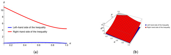
Figure 1. Combined illustration showing (a) 2D and (b) 3D plots for $\Theta \left(\mu \right)=e^{2\mu }$. (a) Two-dimensional plot for $\Theta \left(\mu \right)=e^{2\mu }$, $\delta =0$, $\rho =1$, and $\alpha$ varies from 0 to 1. (b) Three-dimensional plot for $\Theta \left(\mu \right)=e^{2\mu }$, $\alpha$ varies from 0 to 1 and $\rho$ between 1 and 2.

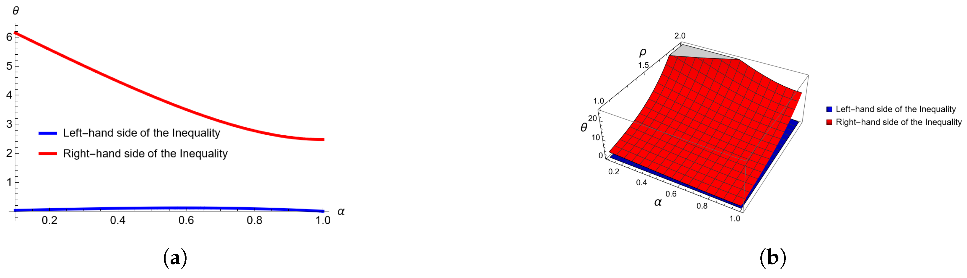
Figure 2. Graphical representation of inequalities of Theorem 3, in Example 1, computed and plotted with Mathematica. (a) Two-dimensional plot for $\Theta \left(\mu \right)={\mu }^6$, $\delta =0$, $\rho =1$, and $\alpha$ varies from 1 to 2. (b) Three-dimensional plot for $\Theta \left(\mu \right)={\mu }^6$, when $\alpha$ varies from 0 to 1 and $\rho$ between 1 and 2.

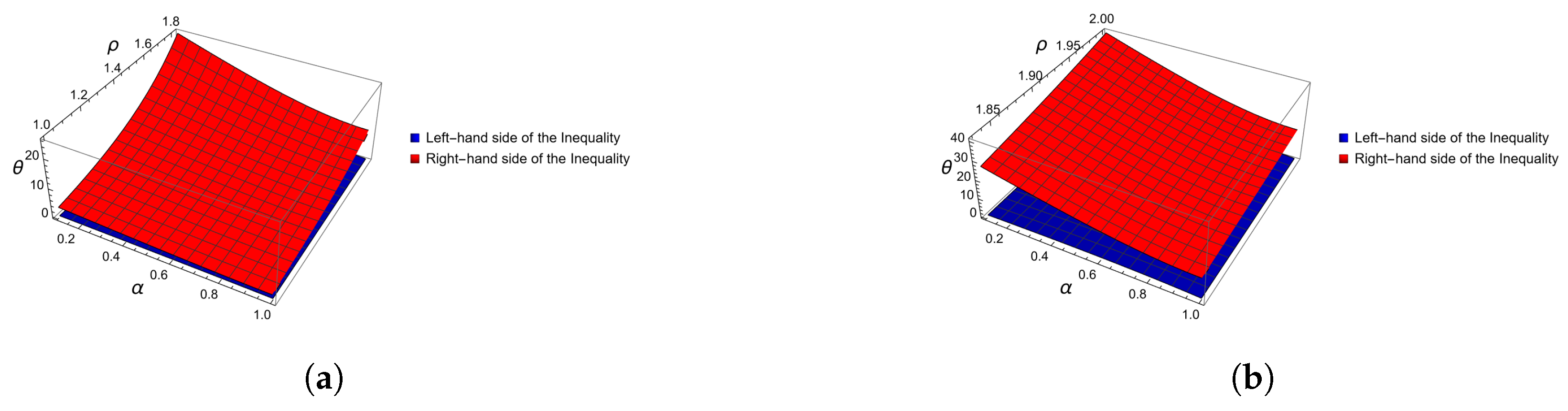
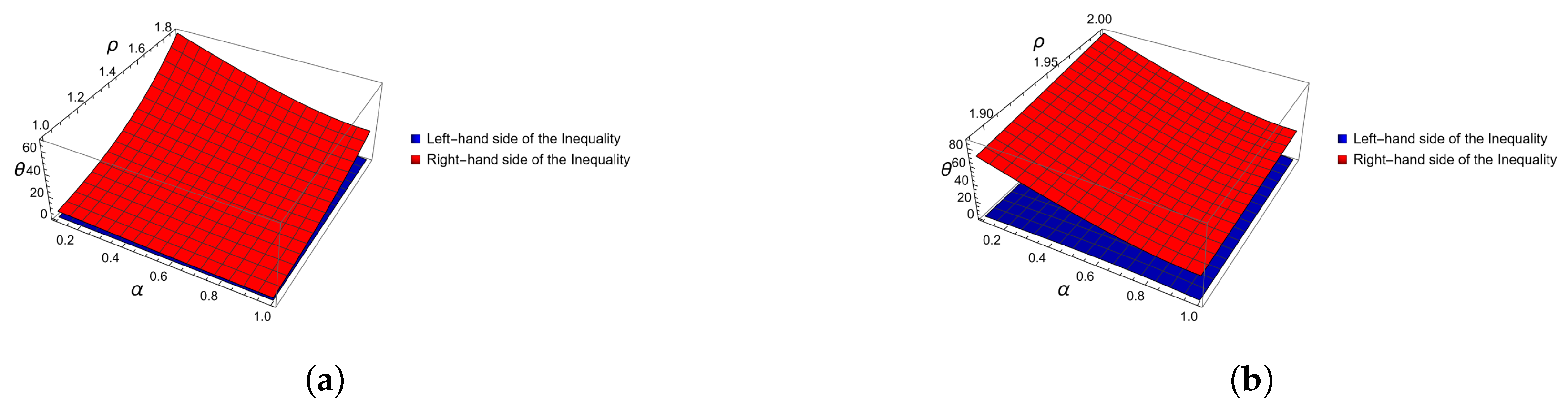
Remark 1.

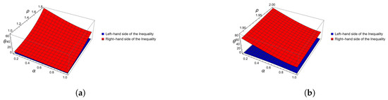
As one can easily observe from the 3D Figure 3 and Figure 4, the left-hand side of (11) in Example 1 is always below the right-hand side. We explored Boole’s inequality behavior about the Caputo fractional integral for Theorem 3. These graphs might show where singularities or breakpoints arise and how an inequality holds under certain conditions.

Figure 3. Graphical representation of inequalities of Theorem 3, in Example 1, computed and plotted with Mathematica. (a) Three-dimensional plot for $\Theta \left(\mu \right)=e^{2\mu }$ when $\alpha$ varies from 0 to 1 and $\rho$ between 1 and $1.82$. (b) Three-dimensional plot for $\Theta \left(\mu \right)=e^{2\mu }$ when $\alpha$ varies from 0 to 1 and $\rho$ between $1.83$ and 2.

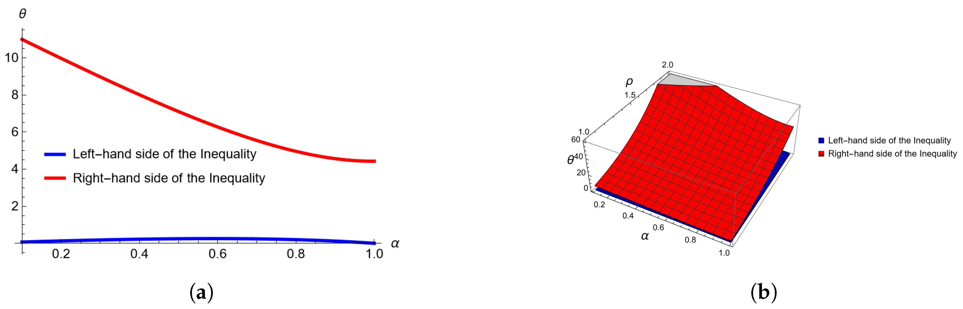
Figure 4. Graphical representation of inequalities of Theorem 3, in Example 1, computed and plotted with Mathematica. (a) Three-dimensional plot for $\Theta \left(\mu \right)={\mu }^6$ when $\alpha$ varies from 0 to 1 and $\rho$ between 1 and $1.88$. (b) Three-dimensional plot for $\Theta \left(\mu \right)={\mu }^6$ when $\alpha$ varies from 0 to 1 and $\rho$ between $1.88$ and 2.

Remark 2.

From Table 1 and Table 2, it can be observed that as α approaches 1, the absolute error significantly improves. This behavior highlights the effectiveness of the proposed method in achieving better accuracy when α is close to 1, thereby demonstrating the robustness of the approach in both classical and multiplicative calculus settings.

4. Conclusions

This paper established a rigorous framework for Boole’s-type inequalities involving diverse classes of functions under the Caputo fractional operator. The analysis was anchored in a fundamental integral identity, the foundation for deriving key results. Boole’s-type inequalities were formulated for differentiable convex functions, bounded functions, and Lipschitzian functions in the context of fractional integrals. The theoretical findings were substantiated through numerical examples and graphical analysis, with computational evidence presented in Table 1 and Table 2. These results highlight the efficacy of the proposed inequalities in providing refined bounds for integral approximations and error estimates. The techniques introduced in this study offer a pathway for future exploration. Potential directions for further research include extending these inequalities to other fractional integral operators, investigating broader classes of convex functions, and employing quantum calculus to develop generalized Boole’s-type inequalities. These extensions have the potential to yield sharper bounds and deeper insights into the interplay between fractional operators and classical inequalities, thereby enriching the theoretical landscape of fractional and quantum calculus.

References

- Miller, K.S.; Ross, B. An Introduction to the Fractional Calculus and Fractional Differential Equations; John Wiley: New York, NY, USA; London, UK, 1993. [Google Scholar]
- Oldham, K.B.; Spanier, J. The Fractional Calculus; Academic Press: New York, NY, USA; London, UK, 1974. [Google Scholar]
- Barkai, E.; Metzler, R.; Klafter, J. From continuous time random walks to the fractional FokkerPlanck equation. Phys. Rev. E 2000, 61, 132–138. [Google Scholar] [CrossRef] [PubMed]
- Metzler, R.; Klafter, J. The random walk’s guide to anomalous diffusion: A fractional dynamics approach. Phys. Rep. 2000, 339, 1–77. [Google Scholar] [CrossRef]
- Kilbas, A.A.; Srivastava, H.M.; Trujillo, J.J. Theory and Applications of Fractional Differential Equations; Elsevier: Amsterdam, The Netherlands, 2006; Volume 204. [Google Scholar]
- Gorenflo, R.; Mainardi, F. Essentials of Fractional Calculus; Maphysto Center: Aarhus, Denmark, 2000. [Google Scholar]
- Euler, L. On transcendental progressions that is, those whose general terms cannot be given algebraically. Comm. Acad. Sci. Petropol. 1999, 5, 36–57. [Google Scholar]
- Ahmad, H.; Seadawy, A.R.; Khan, T.A.; Thounthong, P. Analytic approximate solutions for nonlinear Parabolic dynamical wave equations. J. Taibah Univ. Sci. 2020, 14, 346–358. [Google Scholar] [CrossRef]
- Ahmad, I.; Ahmad, H.; Abouelregal, A.E.; Thounthong, P.; Abdel-Aty, M. Numerical study of integer-order hyperbolic telegraph model in physical and related sciences. Eur. Phys. J. Plus 2020, 135, 1–14. [Google Scholar] [CrossRef]
- Hua, C.; Katugampola, U.N. Hermite–Hadamard and Hermite–Hadamard-Fejér type inequalities for generalized fractional integrals. J. Math. Anal. Appl. 2017, 466, 1274–1291. [Google Scholar]
- Set, E.; Iscan, I.; Sarikaya, M.Z.; Ozdemir, M.E. On new inequalities of Hermite–Hadamard-Fejér type for convex functions via fractional integrals. Appl. Math. Comput. 2015, 259, 875–881. [Google Scholar] [CrossRef]
- Set, E.; Sarikaya, M.Z.; Karakoc, F. Hermite–Hadamard type inequalities for h-convex functions via fractional integrals. Konuralp J. Math. 2016, 4, 254–260. [Google Scholar]
- Iscan, I. Hermite–Hadamard type inequalities for harmonically convex functions. Hacet. J. Math. Stat. 2014, 43, 935–942. [Google Scholar] [CrossRef]
- Gurbuz, M.; Akdemir, A.O.; Rashid, S.; Set, E. Hermite–Hadamard inequality for fractional integrals of Caputo-Fabrizio type and related inequalities. J. Inequal. Appl. 2020, 2020, 172. [Google Scholar] [CrossRef]
- Kwun, Y.C.; Farid, G.; Ullah, S.; Nazeer, W.; Mahreen, K.; Kang, S.M. Inequalities for a unified integral operator and associated results in fractional calculus. IEEE Access 2019, 7, 126283–126292. [Google Scholar] [CrossRef]
- Nguyen, V.T.; Nguyen, V.K.; Quy, P.H. A note on Jesmanowicz conjecture for non-primitive Pythagorean triples. Open J. Math. Sci. 2021, 5, 115–127. [Google Scholar] [CrossRef]
- Yang, X.Z.; Farid, G.; Nazeer, W.; Chu, Y.M.; Dong, C.F. Fractional generalized Hadamard and Fejer-Hadamard inequalities for m-convex functions. AIMS Math. 2020, 5, 6325–6340. [Google Scholar] [CrossRef]
- Farid, G.; Mahreen, K.; Chu, Y.M. Study of inequalities for unified integral operators of generalized convex functions. Open J. Math. Sci. 2021, 5, 80–93. [Google Scholar] [CrossRef]
- Al-Gonah, A.A.; Mohammed, W.K. A new forms of extended hypergeometric functions and their properties. Eng. Appl. Sci. Lett. 2021, 4, 30–41. [Google Scholar]
- Dwilewicz, R.J. A Short History of Convexity. Differential Geometry–Dynamical Systems. 2009. Available online: https://citeseerx.ist.psu.edu/document?repid=rep1&type=pdf&doi=c8726356c97e686242cf8e0a8e21004f854cd321 (accessed on 5 February 2025).
- Dragomir, S.S.; Pearce, C. Selected Topics on Hermite–Hadamard Inequalities and Applications. Science Direct Working Paper 2003, (S1574-0358), 04. Available online: https://ssrn.com/abstract=3158351 (accessed on 5 February 2025).
- O’Connor, J.J.; Robertson, E.F. Jacques Hadamard (1865–1963). MacTutor History of Mathematics Archive; University of St Andrews: St Andrews, UK, 2003. [Google Scholar]
- Mandelbrojt, S.; Schwartz, L. Jacques Hadamard (1865–1963). Bull. Am. Math. Soc. 1965, 71, 107–129. [Google Scholar] [CrossRef]
- Cruz-Uribe, D.; Neugebauer, C.J. Sharp error bounds for the trapezoidal rule and Simpson’s rule. J. Inequal. Pure Appl. Math. 2002, 3, 1–22. [Google Scholar]
- Vivas-Cortez, M.J.; Ali, M.A.; Qaisar, S.; Sial, I.B.; Jansem, S.; Mateen, A. On some new Simpson’s formula type inequalities for convex functions in post-quantum calculus. Symmetry 2021, 13, 2419. [Google Scholar] [CrossRef]
- Hsu, K.C.; Hwang, S.R.; Tseng, K.L. Some extended Simpson-type inequalities and applications. Bull. Iran. Math. Soc. 2017, 43, 409–425. [Google Scholar]
- O’Searcoid, M. Lipschitz Functions, Metric Spaces; Springer Undergraduate Mathematics Series; Springer: Berlin/Heidelberg, Germany; New York, NY, USA, 2006; ISBN 978-1-84628-369-7. [Google Scholar]
- Bartle, R.G.; Sherbert, D.R. Introduction to Real Analysis; Wiley: Hoboken, NJ, USA, 2011. [Google Scholar]
- Baleanu, D.; Mohammed, P.O.; Vivas-Cortez, M.; Rangel-Oliveros, Y. Some modifications in conformable fractional integral inequalities. Adv. Differ. Equ. 2020, 2020, 374. [Google Scholar] [CrossRef]
- Mohammed, P.O.; Abdeljawad, T.; Zeng, S.; Kashuri, A. Fractional Hermite–Hadamard integral inequalities for a new class of convex functions. Symmetry 2020, 12, 1485. [Google Scholar] [CrossRef]
- Moumen, A.; Boulares, H.; Meftah, B.; Shafqat, R.; Alraqad, T.; Ali, E.E.; Khaled, Z. Multiplicatively Simpson-type inequalities via fractional integral. Symmetry 2023, 15, 460. [Google Scholar] [CrossRef]
- Anastassiou, G.A.; Argyros, I.K. Newton-Type Methods on Generalized Banach Spaces and Applications in Fractional Calculus. Algorithms 2015, 8, 832–849. [Google Scholar] [CrossRef]
- Guariglia, E. Riemann zeta fractional derivative-functional equation and link with primes. Adv. Differ. Equ. 2019, 2019, 261. [Google Scholar] [CrossRef]
- Ragusa, M.A. Commutators of fractional integral operators on vanishing-Morrey spaces. J. Glob. Optim. 2008, 40, 361–368. [Google Scholar] [CrossRef]
- Saleh, W.; Lakhdari, A.; Abdeljawad, T.; Meftah, B. On fractional biparameterized Newton-type inequalities. J. Inequal. Appl. 2023, 2023, 122. [Google Scholar] [CrossRef]
- Set, E.; Akdemir, A.O.; Ozdemir, E.M. Simpson-type integral inequalities for convex functions via Riemann–Liouville integrals. Filomat 2017, 31, 4415–4420. [Google Scholar] [CrossRef]
- Sarikaya, M.Z. On Hermite–Hadamard type inequalities for proportional Caputo-hybrid operator. Konuralp J. Math. 2023, 11, 31–39. [Google Scholar]
- Mateen, A.; Zhang, Z.; Toseef, M.; Ali, M.A. A new version of Boole’s formula type inequalities in multiplicative calculus with application to quadrature formula. Bull. Belg. Math. Soc. Simon Stevin 2024, 31, 541–562. [Google Scholar] [CrossRef]
- Sarikaya, M.Z.; Set, E.; Yaldiz, H.; Başak, N. Hermite–Hadamard’s inequalities for fractional integrals and related fractional inequalities. Math. Comput. Model. 2013, 57, 2403–2407. [Google Scholar] [CrossRef]
- Qaisar, S.; Munir, A.; Naeem, M.; Budak, H. Some Caputo-Fabrizio fractional integral inequalities with applications. Filomat 2024, 38, 5905–5923. [Google Scholar]
- Mahajan, Y.; Nagar, H. Fractional Newton-type integral inequalities for the Caputo fractional operator. Math. Methods Appl. Sci. 2024, 48, 5244–5254. [Google Scholar] [CrossRef]
- Ofem, A.E.; Udo, M.O.; Joseph, O.; George, R.; Chikwe, C.F. Convergence analysis of a new implicit iterative scheme and its application to delay Caputo Fractional differential equations. Fractal Fract. 2023, 7, 212. [Google Scholar] [CrossRef]
- Mateen, A.; Zhang, Z.; Budak, H.; Ozcan, S. Some novel inequalities of Weddle’s formula type for Riemann–Liouville fractional integrals with their applications to numerical integration. Chaos Solitons Fractals 2025, 192, 115973. [Google Scholar] [CrossRef]
- Demir, İ.; Tunç, T. A new Approach to Simpson-Type Inequality with Proportional Caputo-Hybrid Operator. Math. Methods Appl. Sci. 2024, 48, 93–106. [Google Scholar] [CrossRef]
- Demir, İ. A new approach of Milne-type inequalities based on proportional Caputo-Hybrid operator. J. Adv. Appl. Comput. Math. 2023, 10, 102–119. [Google Scholar] [CrossRef]
- Almeida, R. A Caputo fractional derivative of a function with respect to another function. Commun. Nonlinear Sci. Numer. Simul. 2017, 44, 460–481. [Google Scholar] [CrossRef]
- Dragomir, S.S. The Ostrowski integral inequality for mappings of bounded variation. Bull. Aust. Math. Soc. 1999, 60, 495–508. [Google Scholar] [CrossRef]
- Dragomir, S.S. On the midpoint quadrature formula for mappings with bounded variation and applications. Kragujev. J. Math. 2000, 22, 13–19. [Google Scholar]
Disclaimer/Publisher’s Note: The statements, opinions and data contained in all publications are solely those of the individual author(s) and contributor(s) and not of MDPI and/or the editor(s). MDPI and/or the editor(s) disclaim responsibility for any injury to people or property resulting from any ideas, methods, instructions or products referred to in the content. |
© 2025 by the authors. Licensee MDPI, Basel, Switzerland. This article is an open access article distributed under the terms and conditions of the Creative Commons Attribution (CC BY) license (https://creativecommons.org/licenses/by/4.0/).