Abstract
Resource-intensiveness often occurs in modern industrial settings; meanwhile, common issues and irregular patterns in production can lead to defects and variations in work-piece dimensions, negatively impacting products and increasing costs. Utilizing traditional process control charts to monitor the process and identify potential anomalies is expensive when intensive resources are needed. To conquer these downsides, algorithms for control chart pattern recognition (CCPR) leverage machine learning models to detect non-normality or normality and ensure product quality is established, and novel approaches that integrate the support vector machine (SVM), random forest (RF), and K-nearest neighbors (KNN) methods with the model selection criterion, named SVM-, RF-, and KNN-CCPR, respectively, are proposed. The three CCPR approaches can save sample resources in the initial process monitoring, improve the weak learner’s ability to recognize non-normal data, and include normality as a special case. Simulation results and case studies show that the proposed SVM-CCPR method outperforms the other two competitors with the highest recognition rate and yields favorable performance for quality control.
Keywords:
K-nearest neighbors; Monte Carlo simulation; pattern recognition; random forest; support vector machines MSC:
62P30
1. Introduction
1.1. Problem Statements and Literature Review
Statistical control charts are efficient tools in statistical process control (SPC) applications for process monitoring and have been widely used in the real world. However, there are still some limitations to the use of statistical control charts. The analysis methods using traditional judgment rules can neither cover all abnormal situations nor provide potential information from previous observations. With the development of SPC and computer technology, the control chart pattern recognition (CCPR) method has overcome these limitations.
Using machine learning models, CCPR is an algorithmic technique that can achieve anomaly detection and quality control in manufacturing processes. The raw data and features, including statistical, shape, and wavelet features, can be two inputs when using CCPR methods. The primary goal of the CCPR method is to actively detect abnormal signals and minimize the costs caused by abnormalities.
Machine learning methods have been used to establish control charts in recent decades. Wang et al. [1] combined a one-sided support vector machine (SVM) control chart with a differential evolution algorithm to monitor multivariate process characteristics. The differential evolution (DE) algorithm is used to estimate the parameters in the SVM under the criterion of minimum mean absolute error (MAE), and the constructed control chart is named the distance-based SVM with the DE algorithm (D-SVM-DE). Ünlü [2] developed a cost-oriented Long Short-term Memory (cost-oriented LSTM) scheme to monitor sequential data to verify the performance of the cost-oriented LSTM method in considering classification and early detection of shifts.
Lee et al. [3] stated that most control chart recognition studies were developed based on the normality assumption of features. However, this assumption usually fails in larger data sets. Miao and Yang [4] used the feature sets of seven basic control chart patterns and seven mixed control chart patterns for training and classification to develop new CCPR methods. Through Monte Carlo simulation experiments, they verified that convolutional neural networks (CNNs) are more effective compared to other methods. Other recent studies using CNNs for CCPR can be found, for example, Fuqua and Razzaghi [5], Cheng et al. [6], Cheng et al. [7], and Xue et al. [8].
Yu and Zhang [9] combined the fusion feature reduction (FFR) and the genetic algorithm-based convolutional LSTM network (GACLN) methods to develop SPC tools. Tian et al. [10] used new deep learning methods to address control problems caused by data imbalances in manufacturing processes. Alwan et al. [11] proposed an ensemble CCPR method focusing on -chart patterns of small process variations. The ensemble classifier consists of five machine learning algorithms, including the decision tree, artificial neural network, linear SVM, Gaussian SVM, and KNN. Sabahno and Niaki [12] used two different input scenarios and training methods to propose machine learning control charts using the artificial neural network, SVM, and RF methods. The goals are to detect the out-of-control signal and identify the process parameters for the out-of-control signal. Yeganeh et al. [13] established machine learning charts for network surveillance problems. The machine learning charts aim to monitor the number of communications between the nodes. Simulation results revealed that the proposed machine learning charts outperformed conventional competitors. Pham and Oztemel [14] combined heuristic multilayer perceptrons to construct a hybrid system for online monitoring of CCPR. They used an integrated module for decision-making. Li and He [15] proposed a multiscale ensemble classifier for CCPR. They combined the ordinal pattern features of control chart pattern data and weighted ordinal pattern features to establish the ensemble classifier. Moreover, they used Monte Carlo simulations to evaluate the performance of their proposed method.
1.2. The Motivation
Existing CCPR methods for process monitoring were established based on the normality assumption of quality variables. In today’s manufacturing, it not only allows for prompt corrections but also saves time and observation costs. It is difficult to cumulate enough sample resource to implement a CCPR method for process monitoring in the initial stage. Simulating all the in-control and out-of-control scenarios as the initial samples to implement CCPR methods can be a solution. Then, the process can be continually monitored using the CCPR method and sample resources cumulated over time till a big sample has been accumulated. Next, the CCPR methods must be retrained for process control based on the big sample.
It is commonly assumed that the process model is addressed by , where and is a known constant. In reality, the distribution of can be symmetric but has either a heavy or thin tail depending on the production conditions. The normal distribution frequently indicates the distribution of having a thin tail. In this work, we combine the model selection method with the SVM, RF, and KNN methods to implement the CCPR method when the data volume at the initial monitoring state is insufficient to well drive a CCPR or deep learning method. Before distinguishing whether the process has a heavy or thin tail, model selection is first used to identify the source distribution. next, we develop the proposed CCPR methods for process monitoring based on the simulated data. To the best of our knowledge, no existing CCPR method with model selection has been studied.
The new CCPR methods can improve the accuracy and efficiency for different CCPRs, for example, the patterns using the model or parameters proposed by Zan et al. [16]. We assume the process distribution to be the Student t distribution, which covers the normal distribution as a special case. We use “t distribution” to denote “Student t distribution” here and after for simplicity. The t distribution is a family of symmetric ones, whose tails can be heavy or thin depending on the degrees of freedom. Once the original distribution of the data is identified using the proposed model selection method, the required sample resources for training the machine learning model can be generated from the target models. If we identify the degrees of freedom of the t distribution based on the available samples being 30 or larger, the t distribution can be regarded as the standard normal distribution. Therefore, this study can accommodate both normal and t distributions, expanding the application scope of the model.
The SVM is a powerful machine learning tool. It can act as a smart classifier that helps the decision-maker reach a satisfactory decision based on data. The strengths and implementation of SVMs are discussed in Section 2.2. In summary, this study analyzes the following two situations:
- 1
- Applying model selection and SVM, RF, and KNN methods to develop the proposed CCPR method.
- 2
- Investigating the recognition quality of the control chart based on the conditions of generated data.
The model selection method can also be used for weak learners other than the SVM, RF and KNN methods in machine learning. The novelty lies in combining the model selection with weaker learners in machine learning to enhance their ability to control chart pattern recognition. In this study, the weaker learners, including SVM, RF, and KNN, are included to combine with the model selection method to develop the proposed methods. The new methods are denoted by SVM-CCPR, RF-CCPR, and KNN-CCPR methods. Intensive Monte Carlo simulations show that the SVM-CCPR method outperforms the RF-CCPR and KNN-CCPR methods based on the recognition rate.
The rest of this article is organized as follows: In Section 2, the six control chart patterns used in this study are discussed and a new SVM-CCPR method that combines the model selection method and SVM is introduced. In Section 3, the performance of the proposed CCPR method is verified using Monte Carlo simulation. Moreover, the RF-CCPR and KNN-CCPR methods are introduced as the competitors to the SVM-CCPR method, and their performances are compared in parallel using Monte Carlo simulations. An example is used for demonstration in Section 4. Some concluding remarks are given in Section 5.
2. Control Chart Patterns and the Proposed CCPR Method
2.1. Data Patterns for Identification
Without loss of generalization, let the in-control production process under monitoring follow the process defined in Case I:
- Case I: The in-control process is defined bywhere is the in-control process mean and denotes the t distribution with degrees of freedom . When , the probability distribution of random errors can be approximated by the standard normal distribution, denoted by . The probability density function of the t distribution is defined by
The t distribution has a mean 0 if and variance if .
Let the out-of-control production processes follow one of Cases II to V.
- Case II: The process of the mean shift is defined bywhere and a is a constant.
- Case III: The process of the standard deviation shift is defined bywhere is a positive constant. Because means the standard deviation is reduced from the nominal level, a reduced standard deviation indicates the process is improved. Hence, only the case of is considered in this study to indicate that the process out of control due to the standard deviation shift.
- Case IV: The process of the mean and standard deviation shifts is defined by
- Case V: The process of the mean drift and standard deviation shift is defined bywhere , , and denotes the standard normal distribution. The charts of Case I to Case V can be illustrated using generated samples.
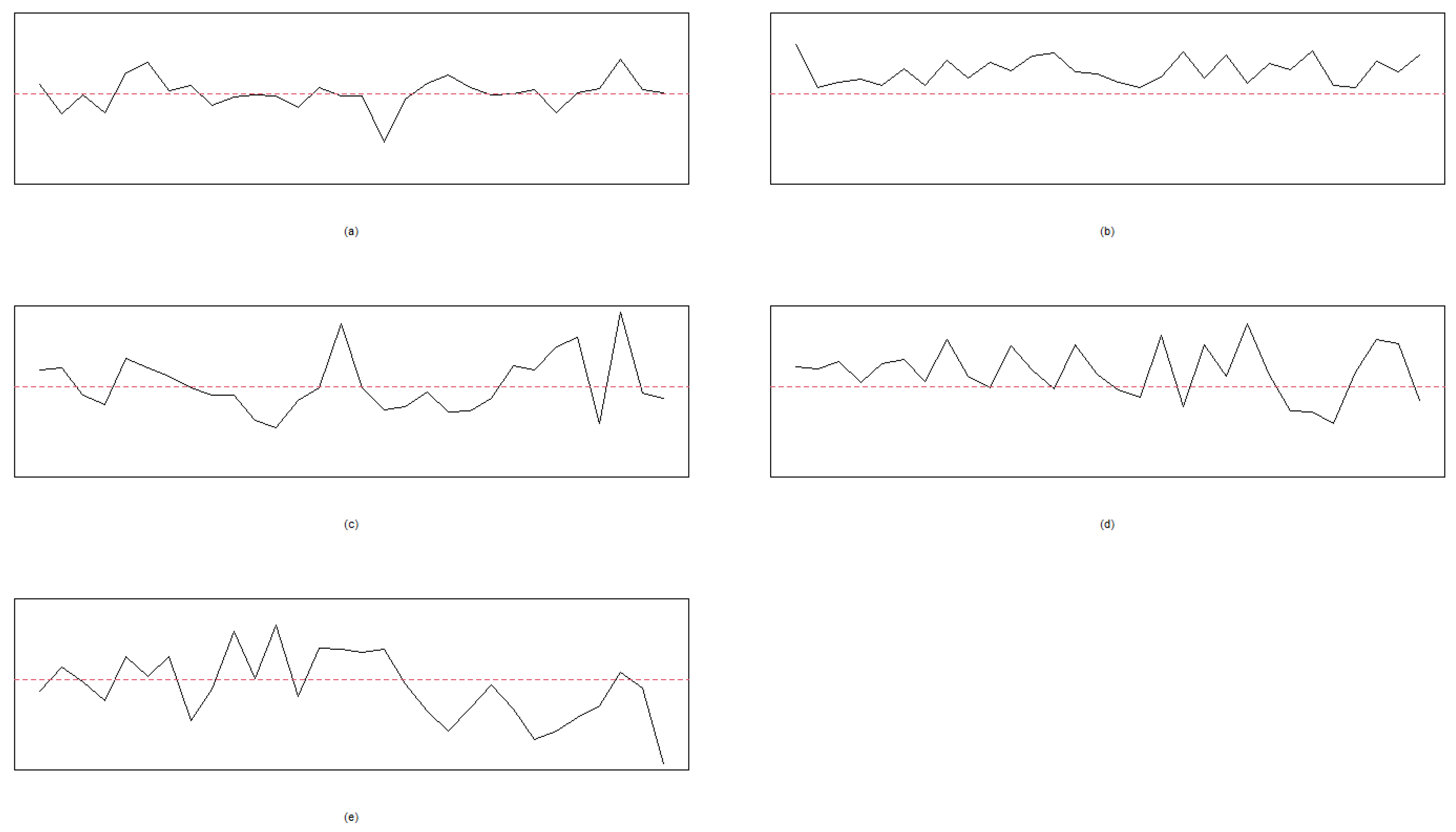
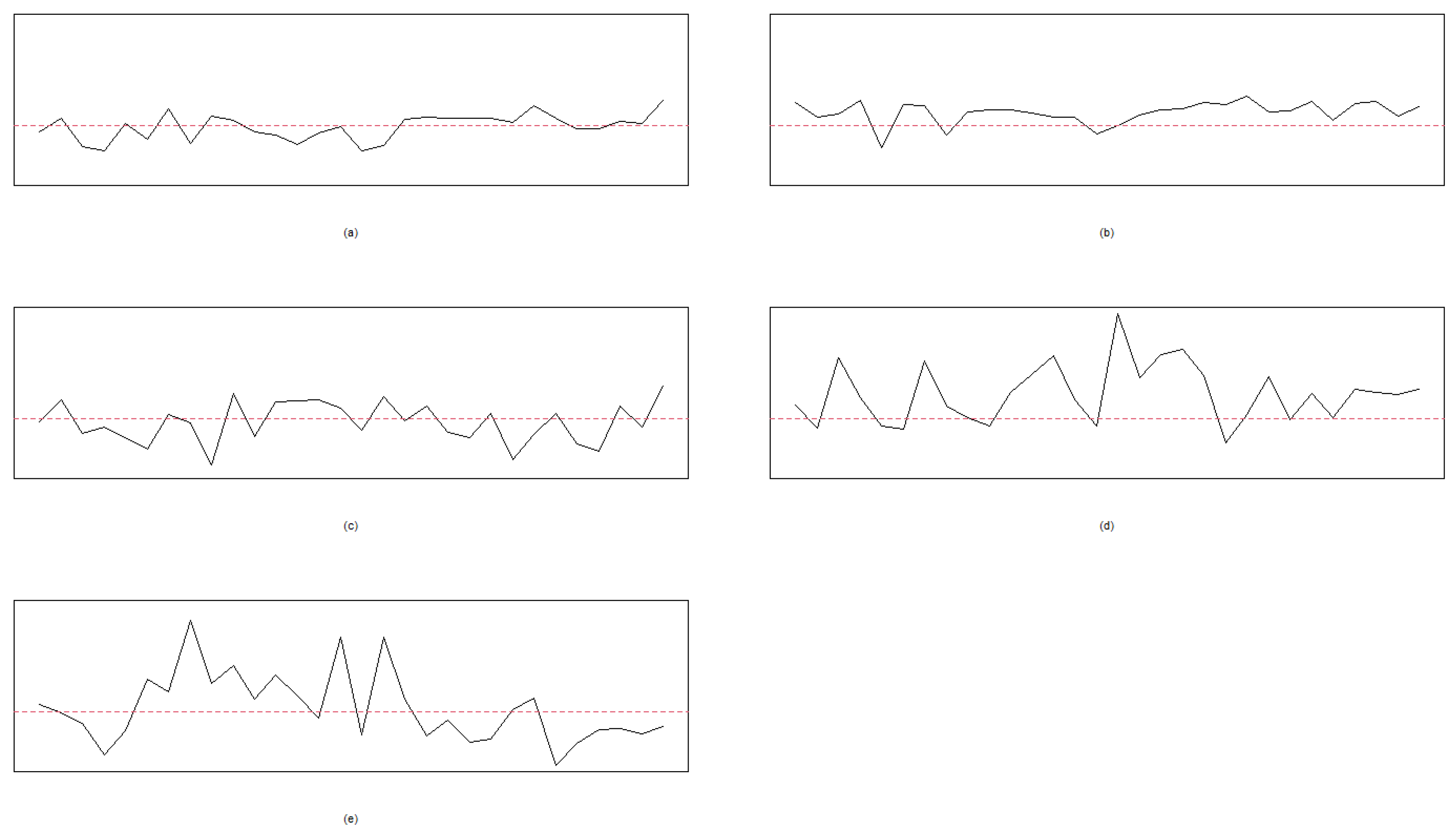
Let , , and the process mean be given in the interval of [20, 30]. That is, we randomly select a value from the interval of [20, 30] for . Thirty points are used for plotting each chart for Cases I, II, III, IV, and V, respectively. Moreover, and are used to indicate that the random error of the process follows the t and standard normal distributions, respectively. The resulting patterns of ten cases under the normal and t-distributed random errors are given in Figure 1 and Figure 2, respectively. Figure 1 and Figure 2 are generated using the R codes developed by the authors.
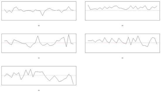
Figure 1.
The random errors follow with 30 points in each chart: (a) Case I, (b) Case II, (c) Case III, (d) Case IV, and (e) Case V. The dashed line is the mean level, .
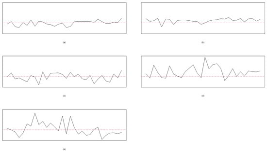
Figure 2.
The random errors follow with 30 points in each chart: (a) Case I, (b) Case II, (c) Case III, (d) Case IV, and (e) Case V. The dashed line is the mean level, .
2.2. The Model-Selection-Based CCPR Methods
In the applications of machine learning and data science, the SVM is incredibly versatile, and the decision-maker can use an SVM to obtain good classification results for many tasks. The strengths of the SVM are addressed as follows:
- High-dimensional data commonly exist in the real world. SVMs are an excellent tool for handling high-dimensional data and searching out the best way to separate the data for classification.
- SVMs can perform linear and nonlinear separations for data classifications. In many instances, data cannot easily be separable by a straight line. SVM methods can use kernel tricks to add another dimension to the data. Such tricks make SVMs efficient in separating nonlinear data when the data resource is limited.
- SVMs consider the balance between obtaining a high prediction accuracy of classification and the reduction of the model overfitting.
- SVMs can be used in different applications, such as biology, finance, business, and education. SVM methods help decision-makers understand and classify complex data.
Linear and nonlinear SVM methods were used to train the proposed CCPR method. The SVM is one of the supervised learning algorithms for classification. We denote the data set by
where denotes a k-dimension vector of features, denotes the binary response variable, and N denotes the sample size. The goal of the linear SVM algorithm is to create the best line or decision boundary that can produce the best classification to predict the new data point in the correct category. We can call the best decision boundary a hyperplane denoted by , where is the normal vector of the hyperplane and b is the intercept of the training sample. The SVM uses the extreme points/vectors to create the hyperplane. The optimal hyperplane can be obtained if the following two conditions hold.
The optimal solutions of and b can be obtained to minimize the target function defined by
where is the Lagrange multiplier. Ranaee et al. [17] comprehensively explained the linear SVM method.
In practical applications, the data set can be complex, and a linear SVM often cannot have good accuracy to separate categorical data for some instances. To fill this gap, nonlinear SVMs can be an alternative solution to perform the classification. The principle behind the nonlinear SVM is to project the original data into a higher-dimensional feature space through a nonlinear transformation, where a separating hyperplane can be constructed in the feature space.
Linear separation means that users can use a straight line to separate two groups of data points; that is, users can draw a straight line on an area of a figure to separate two categories. Nonlinear separation, on the other hand, occurs when drawing a straight line to separate data is unavailable. For complex data, an SVM uses kernel tricks to improve the classification quality. The idea of kernel tricks is to transform data into a higher-dimension space using a kernel function. Then, a hyperplane is constructed with the best separation while maximizing the margin between the two categories. Finally, new data points with the same kernel transformation will be classified. The decision boundary can be determined based on the location of the transformed data in the hyperplane. The kernel tricks make it possible to separate data using a hyperplane to improve the classification quality by using a straight line in the original space.
Data transformation can be carried out using four kernel functions, which include the linear, polynomial, radial basis function (RBF), and sigmoid kernel functions. Smola et al. [18] have more illustrations. Each kernel function can be used with different calculation methods and parameters. Table 1 presents four popular kernel functions to implement an SVM. Let and denote data points, c be a constant, and be a hyperparameter to control the width of the radial basis kernel.

Table 1.
The kernel functions for implementing SVM methods.
Assume that the in-control process is defined by Case I and four out-of-control scenarios by Cases II–V. The distributions of error terms are symmetric. If the quality of the process cannot be ascertained, then the distribution can have heavy or thin tails. One solution is combining all ten cases, five for normal distributed random error terms and the other five for t-distributed error terms, similar to those shown in Figure 1 and Figure 2, to train SVMs. However, such a method requires huge sample resources and could delay the online monitoring of SPC because of the high time required to accumulate sample resources. A better method is to select a probability model for the quality variable after collecting fewer sample resources from the initial samples. After data transformation, identify the data distribution of random error terms based on the working samples. Then, perform a data augment to generate in- and out-of-control samples based on the setting of in-control and out-of-control mathematical models as pseudo samples. Then, the SVM will be trained with pseudo samples.
Let the levels of the response variable be q, where q is a positive integer equal to or larger than 2. The one-against-one approach is used, in which binary classifiers are trained. Then, the new observation can be classified based on the majority vote. In this study, the proposed CCPR method can be established with Algorithm 1.
The SVM with the RBF kernel function can have a better classification efficiency with less parameter adjustment for high-dimensional data, see Lu et al. [19]. In this study, a nonlinear SVM is implemented with the RBF kernel function. Let denote the total number of correctly recognized samples based on m samples. The metric of the rate of correct classification (ROCC) is defined by
The ROCC in Equation (12) is used to evaluate the accuracy of the proposed method. The larger the ROCC is, the better quality the CCPR method has. Replacing the SVM method with RF and KNN methods in Step 6, the SVM-CCPR method becomes RF-CCPR and KNN-CCPR methods, respectively.
The RF method is an ensemble learning technique, primarily used for implementing classification and regression tasks. RF was built based on the concept of decision trees, in which multiple individual decision trees are created. Then, their predictions are aggregated for the final decision. In RF, many decision trees are trained based on different bootstrapped subsets of the training data. Bootstrapping means that data points are sampled randomly, with replacement, to create different training sets for each tree. Each tree has a different view of the train data to reduce overfitting and improve generalization. For the classification task, the final prediction is determined by majority voting. RF can effectively handle large data sets with many features and assess the importance of features in predicting the response variable. Moreover, RF can model complex nonlinear relationships in data. Because of using the bagging technique for implementation, RF can be time-consuming in computation.
| Algorithm 1: The implementation of the SVM-CCPR method. |
|
The KNN can be implemented using a simple and intuitive machine learning algorithm for classification and regression tasks. To implement KNN, we do not need to build a model or make any assumptions about the data. Instead, KNN memorizes the training data and makes predictions regarding those data at the time of query. We can use a distance metric to measure how similar data points are to each other in the feature space. For each query point, the KNN finds the number of nearest neighbors based on the distance metric. KNN is easy to implement, and KNN is effective for smaller data sets with fewer features. However, the KNN asks for evaluating the distance to every point in the training data for prediction, so it can become time-consuming for large data sets. If the data set has many irrelevant features, the KNN becomes less efficient. In high-dimensional spaces of many features, the concept of nearness is less meaningful, and this fact makes KNN less efficient, too.
3. Performance Evaluation for the Proposed CCPR Method
Monte Carlo simulations are conducted to compare the performance of the proposed SVM-CCPR, RF-CCPR, and KNN-CCPR methods. The strengths of the integrated CCPR methods (integrating the model selection technique and CCPR) and the guidelines for using them are also studied in this section.
Parameter Settings
To implement the Monte Carlo simulation study for the proposed CCPR methods, Case I to Case V in Section 2.1 are used to generate random samples with the following parameters:
- The number of samples: , 50, 80, 100, 200, 300, 500, and 800. These values of m are used to evaluate the impact of the number of sample control charts on the recognition rate of the proposed CCPR methods.
- The sample size in each control chart: Each case is established with different sample sizes. In this simulation study, , 50, 100 are considered to evaluate the impact of sample size on the recognition rate of the proposed CCPR methods.
- Candidate distributions for model selection: The degrees of freedom and 20 are considered for the non-normal distributed cases with different heavy-tailed levels. Moreover, the normal distributed samples are also used in the simulation study by using the Student t distribution with .
- The source codes and packages for Monte Carlo simulation: R codes and the packages e1071, randomForest, and class are prepared to implement the SVM, RF, and KNN methods.
- The proportion of the training sample in the complete sample: Eighty percent of the points in the complete sample are randomly selected for the training sample for training the SVM, RF, and KNN models. Then, the trained models and the features in the test sample, which is composed of the other twenty percent points in the complete sample, are used to predict the responses, which are either −1 or 1.
- The number of iterative runs: One thousand repetitions are used to evaluate the values of ROCC.
To use the R package to implement the SVM algorithm with RBF, the hyperparameter and the penalty parameter need to be tuned based on data to obtain an SVM for classification. can be used to shape the decision boundary to assemble and cluster similar data points. Moreover, the penalty parameter is used to control the penalty of misclassification. In this study, the value of is set to the inverse of the data dimension. After the simulation study, we suggest using the penalty parameter 1 and the inverse of the data dimension for to implement the SVM method.
The ROCC defined in Equation (12) is used as the metric to evaluate the quality of the proposed method. The performance evaluation is not only to identify whether the process is out of control or in control; we also ask whether the SVM-CCPR method identifies the right case classification. To verify the performance of the model-selection-based CCPR method, competitors, the RF-CCPR and KNN-CCPR methods, are considered in the simulation study.
Five hundred trees of bagging are considered to implement the RF method; each tree can have and k features for performance comparison. k is the number of features in the data set. That is, partial or all features are considered to implement bagging RF. For simplicity, we use RF1 and RF2 to denote the RF-CCPR method with and k features, respectively.
and nearest neighbors are considered to implement the KNN method. The Euclidean distance is used to measure the similarity among sample points. For simplicity, we use KNN1 and KNN2 to denote the KNN-CCPR method with and nearest neighbors, respectively.
Existing works have indicated the superiority of SVMs for process monitoring under a normality assumption. If the distribution of the process variable was symmetric with heavy tails, then the performance of the SVM-CCPR, RF-CCPR, and KNN-CCPR methods was not studied to the best of our best knowledge. In this study, simulations were conducted, and the ROCC was computed on an average of 1000 repetitions to remove the effect of random error. All simulation results are summarized in Table 2, Table 3 and Table 4.
Table 2.
The values of ROCC of the proposed CCPR methods for .
Table 3.
The values of ROCC of the proposed CCPR methods for .
Table 4.
The values of ROCC of the proposed CCPR methods for .
From Table 2, we can see that the lower and upper bounds of ROCC for the SVM-CCPR method are about 87% and 94%, respectively. Moreover, the ROCC of the SVM-CCPR is bigger than 90% if . In Table 3, we find that the ROCC of the SVM-CCPR method is greater than 91.7%. The findings are interesting. If we can cumulate 1500 from the process to implement the SVM-CCPR methods, then putting 50 points for each chart with for each case can have a better performance than putting 30 points with . Table 3 also shows that by putting 50 points in each chart with or more, the ROCC of the SVM-CCPR method is greater than 95%, which indicates a good performance of a good SVM-CCPR design. Table 4 shows that putting 100 points in each chart with for each case can have an ROCC larger than 96%. In summary, with an ROCC of at least 95%, the combinations of and or and can be references with which to implement the SVM-CCPR method. We also see that the SVM-CCPR method can have a good performance in process monitoring if the distribution of the random error terms is symmetric with heavy or thinned tails.
Table 2, Table 3 and Table 4 also show that the RF-CCPR method performs worse than the SVM-CCPR method for all parameter settings, and the KNN-CCPR performs worst among all competitors. RF is another popular weaker learner in machine learning applications. Moreover, the design of RF using features to construct subtrees (denoted by RF1) is better than the design of RF using all p features to construct subtrees (denoted by RF2). If we expect the ROCC of the RF-CCPR method to be larger than 95%, at least 4000 sample points must be accumulated with and to implement the RF-CCPR method that is using features to construct subtrees. The values of ROCC for the KNN1-CCPR and KNN2-CCPR methods are below 60% even though the value of m increased to 800. We do not recommend using the KNN method for CCPR. The value of ROCC can increase over m. However, the increment of ROCC is insignificant compared with that based on the SVM-CCPR, RF1-CCPR, and RF2-CCPR methods.
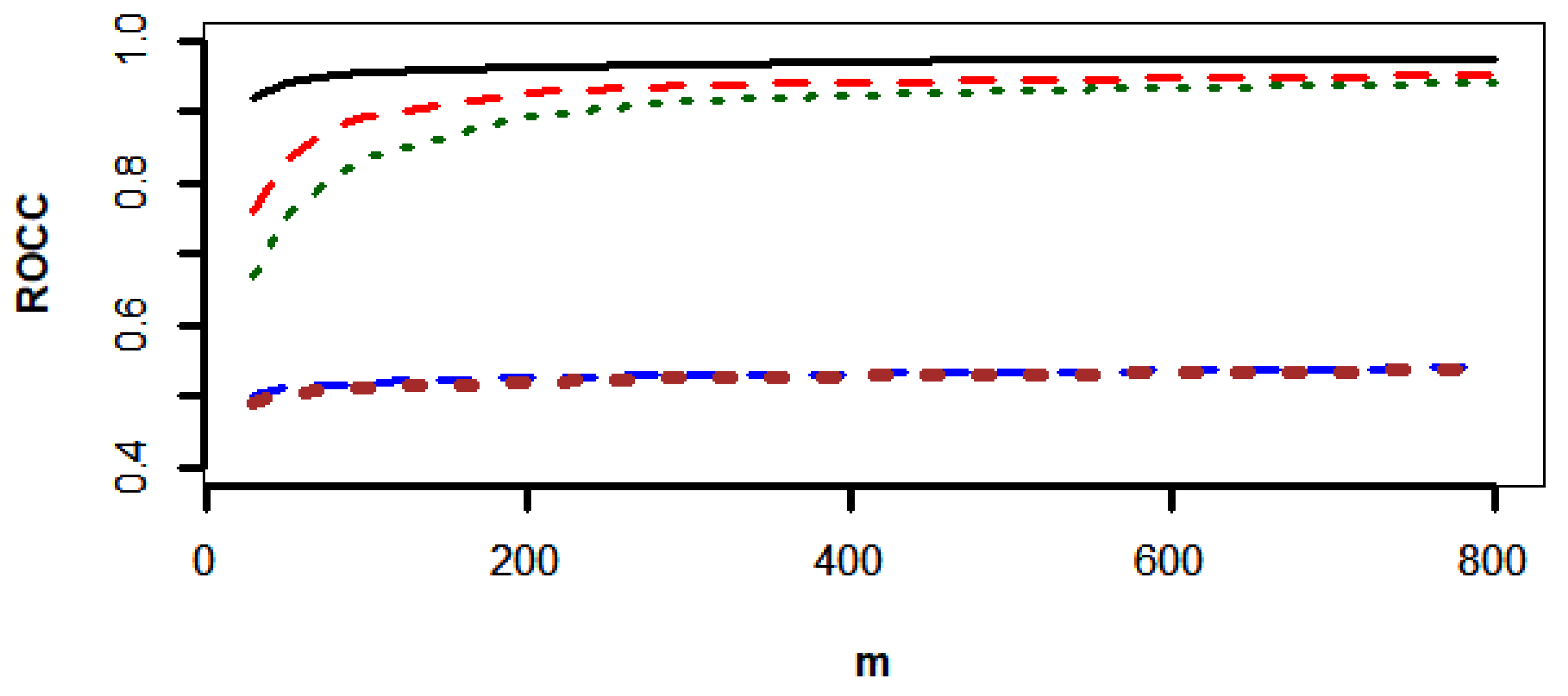
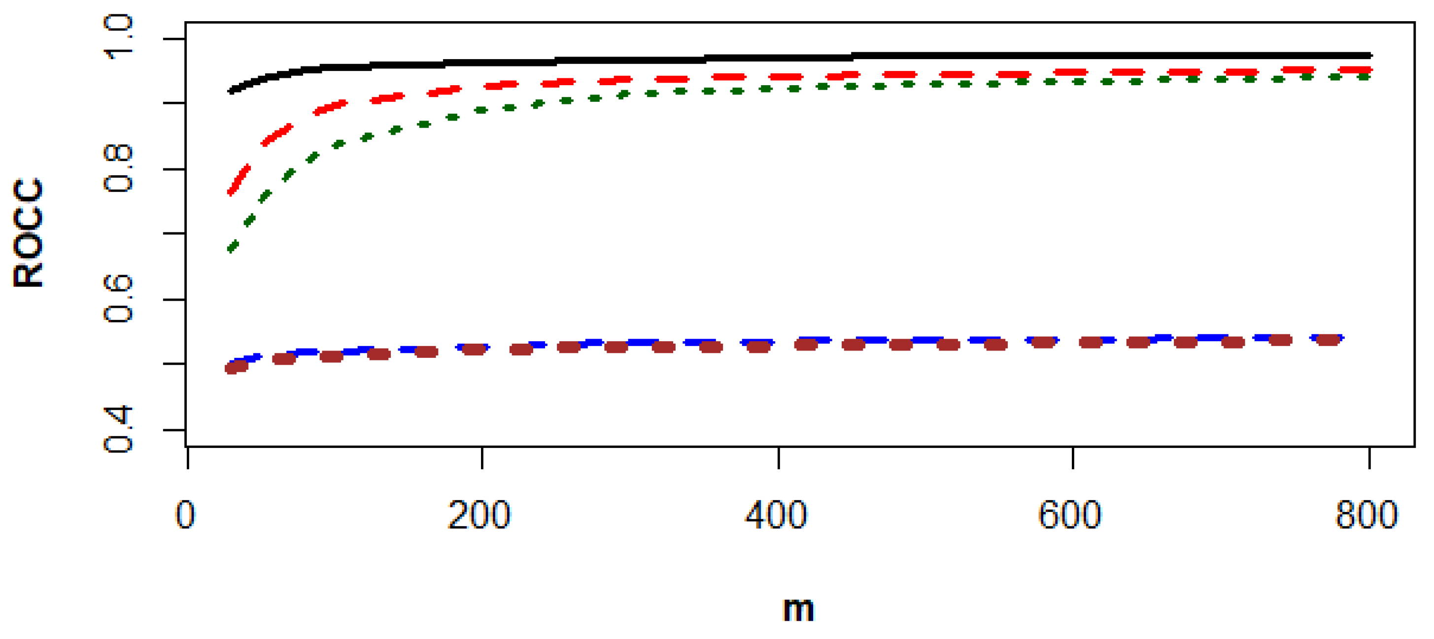
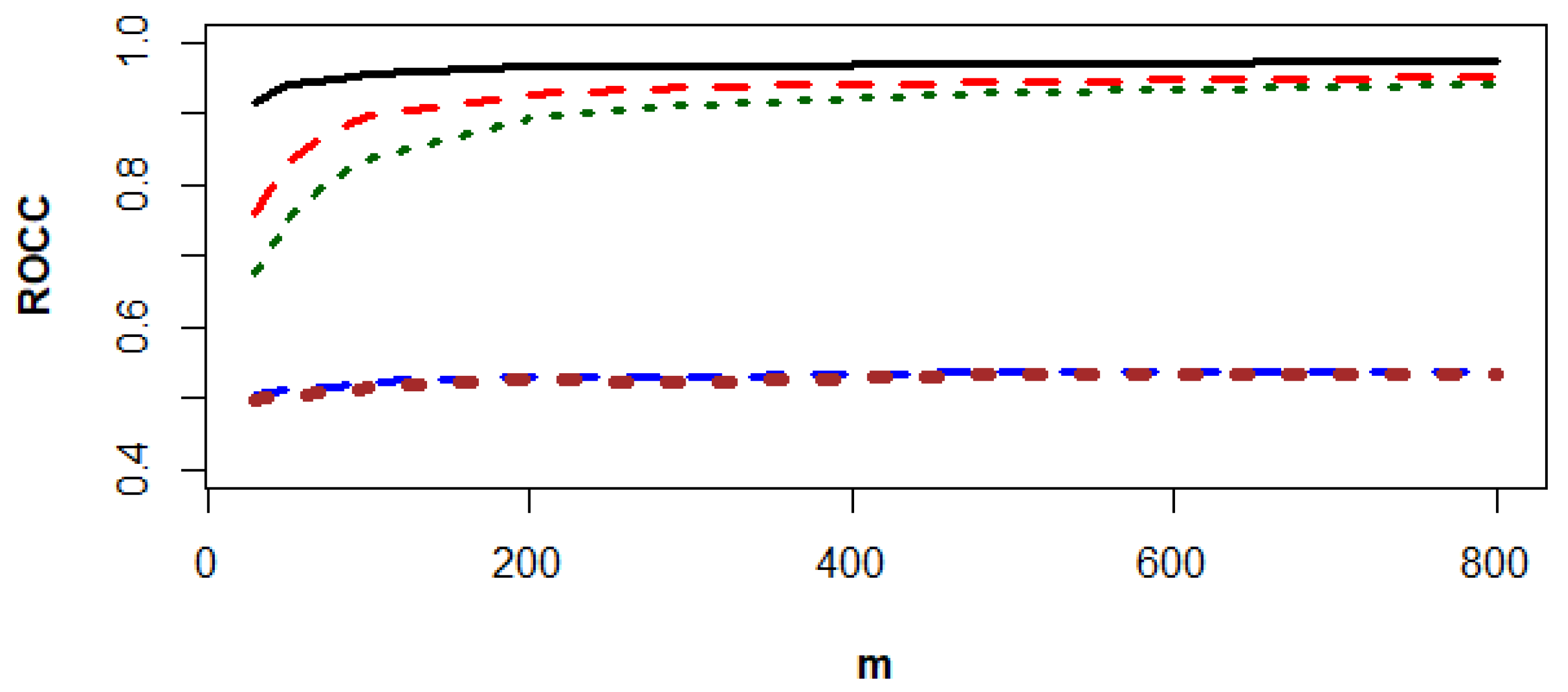
Figure 3, Figure 4 and Figure 5 show that the SVN-CCPR method beats the other competitors, and the gaps between the ROCC of the SVN-CCPR, RF1-CCPR, and RF2-CCPR methods decreases as m increases. The gap decrement between the KNN1-CCPR and KNN2-CCPR methods is insignificant.
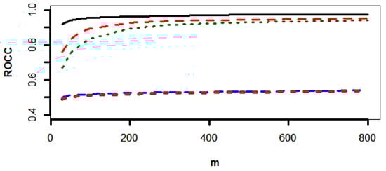
Figure 3.
The values of ROCC for SVM-CCPR (black solid line), RF1-CCPR (red dashes), RF2-CCPR (green dots), KNN1-CCPR (blue dashes), and KNN2-CCPR (brown dots) methods based on the data generated from and .
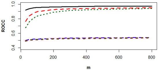
Figure 4.
The values of ROCC for SVM-CCPR (black solid line), RF1-CCPR (red dashes), RF2-CCPR (green dots), KNN1-CCPR (blue dashes), and KNN2-CCPR (brown dots) methods based on the data generated from and .
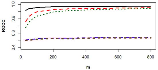
Figure 5.
The values of ROCC for SVM-CCPR (black solid line), RF1-CCPR (red dashes), RF2-CCPR (green dots), KNN1-CCPR (blue dashes), and KNN2-CCPR (brown dots) methods based on the data generated from and .
In the early monitoring stage of quality control, users can generate a small in-control sample, for example, 150 points as the traditional SPC suggestion with N = 5, m = 20 to 30; see Montgomery [20]. We normalize the in-control sample and perform the model selection using the AIC method for the normalized points based on the Student t distribution with the degrees of freedom in the interval between 15 and 30 to obtain the candidate of the distribution of random errors. After the distribution of random errors is determined, we generate 4000 points, then separate all sample points in time order and put 50 points in each chart. We combine all 80 charts of each case to train the proposed SVM-CCPR method for process monitoring.
4. An Example
In this section, we use the printed circuit board (PCB) example in Cheng et al. [6] to illustrate the proposed CCPR method for process monitoring. The data involve various processes of chemical solution monitoring, such as electroplating, etching, and cleaning. Chemical concentrations may exhibit abnormal changes because of various reasons, such as initial bath preparation, dosage calculation errors, incorrect dosage formulas, irregular manual dosing operations, and failures in automatic dosing systems. Irregular demand changes can lead to abnormal concentration variations, and timely detection of issues at an early stage when the sample size is small can reduce the burden on engineers for control chart data analysis.
Cheng et al. [6] reported a sample of size 32 with seven types of patterns, and 15 samples were reported for each pattern, including the patterns of a normal situation (NOR), systematic variations (SYS), a cycle (CYC), an upward trend (UT), a downward trend (DT), an upward shift (US), and a downward shift (DS). The mathematical forms of the seven patterns are summarized as follows:
- Case E1, NOR:where , are random errors. In this study, we consider , , , and can be determined using the AIC method based on the available in-control samples.
- Case E2, SYS:where and denote the starting time and shift size of the systematic variation, respectively. determines the location of the first observation and can be a random value in the interval of 0 to 1.
- Case E3, CYC:where and are the amplitude of the cycle and the length of the amplitude, respectively.
- Case E4, the trends of UT and DT:where is the slope of the trend. is used to determine the direction of the trend. If , the trend is UT, and it is DT otherwise.
- Case E5, Shifts of US and DS:where is the shift size. determines the shift direction. If , the shift is US, and it is DS otherwise.
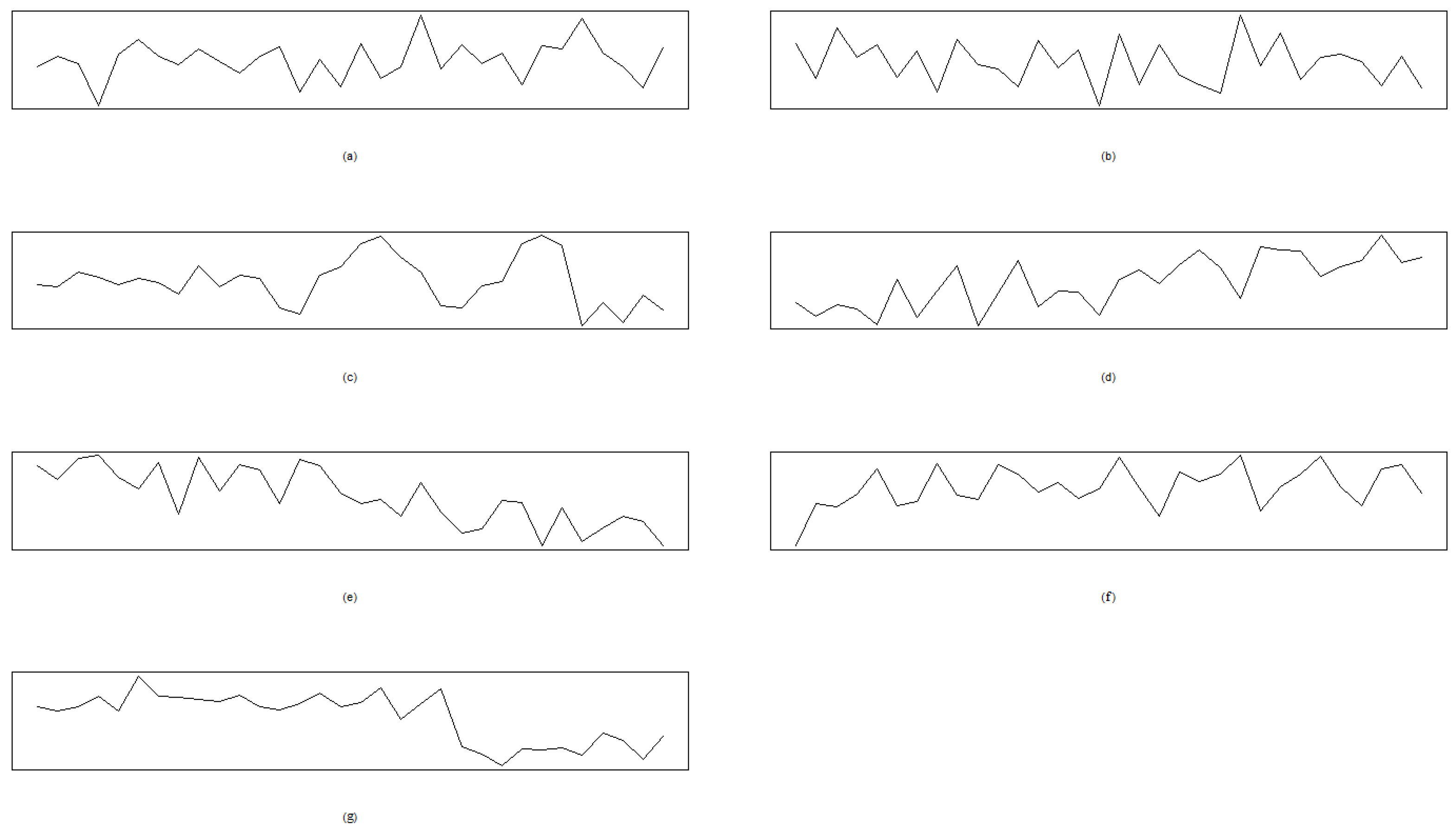
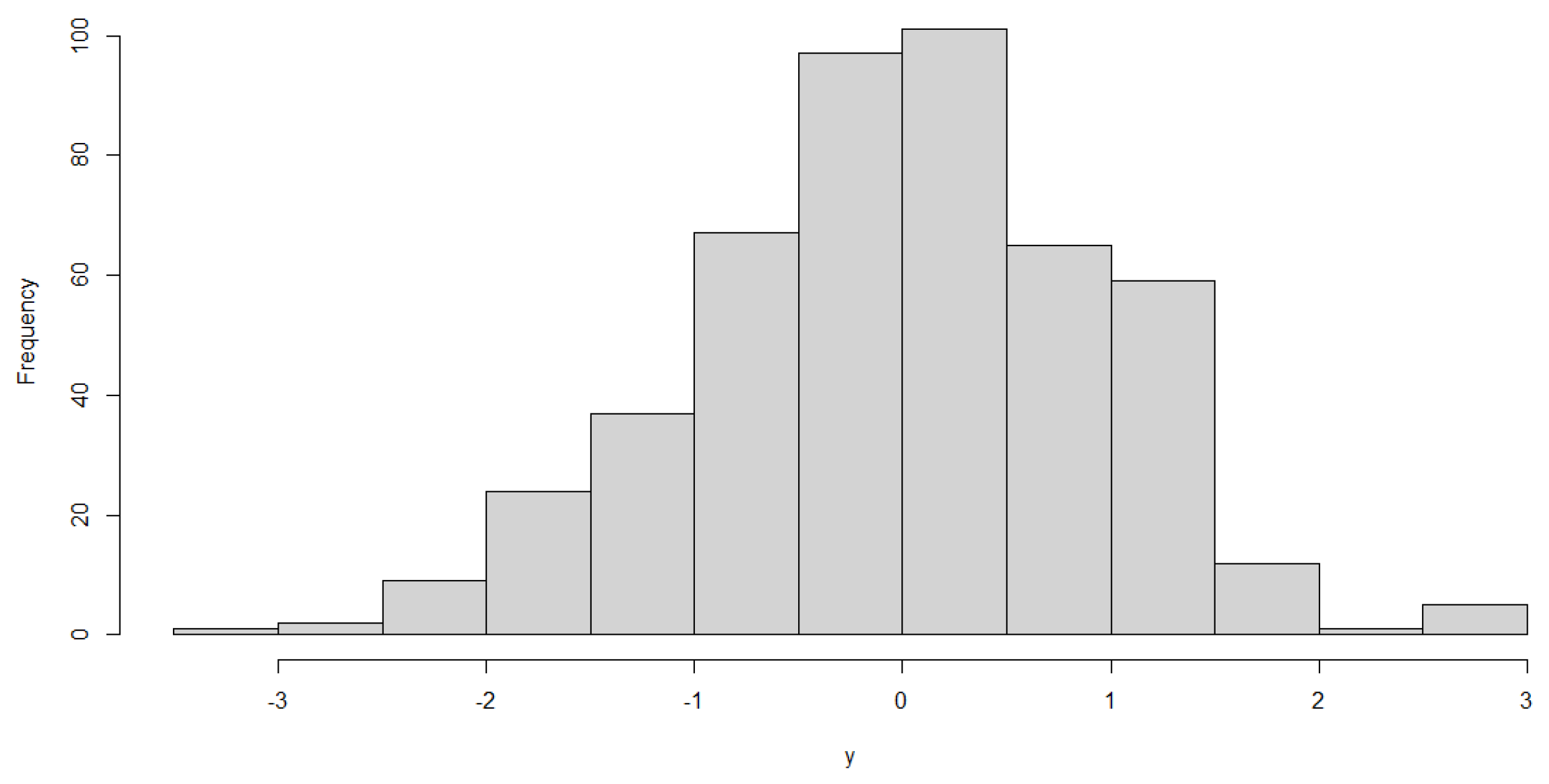
To generate the data from the seven patterns, we take the ranges of the parameters of this example in Table 5. The Phase I in-control sample with and is used to plot the quantile-to-quantile (QQ) plot and histogram to test the normality. Figure 6 presents the seven patterns of Case E1 to Case E5, and the QQ plot reported in Figure 7 indicates a good model fitting and shows that the normal distribution can be the right candidate distribution to characterize the PCB data set. The histogram in Figure 8 also supports that the distribution of Phase I in the control sample is symmetric.
Table 5.
The parameters of the PCB example.
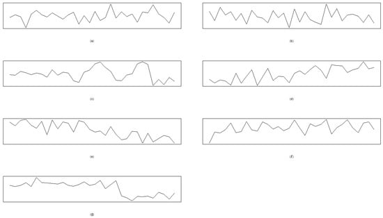
Figure 6.
The seven patterns of the PCB example. (a) Case E1: NOR. (b) Case E2: SYS. (c) Case E3: CYC. (d) Case E4: UT. (e) Case E4: DT. (f) Case E5: The shift of US. (g) Case E5: The shift of DS.
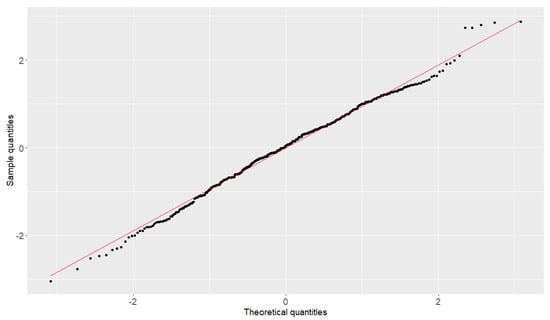
Figure 7.
The quantity–to–quantity plot of the PCB sample.

Figure 8.
The histogram of the PCB sample.
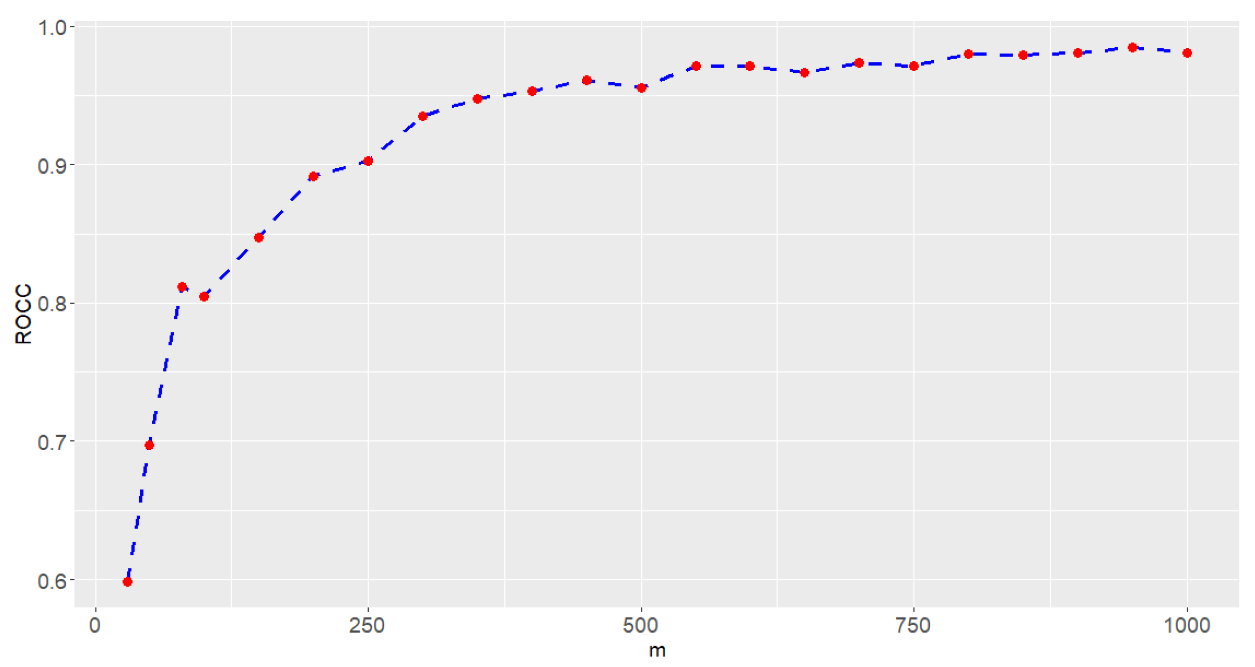
Based on , we generate different numbers of m to evaluate the ROCC for this example. Each chart of Case E1 to Case E5 is generated based on 32 sample points. In this study, , 50, 80, 100, 150, 200, 250, 300, 350, 400, 450, 500, 550, 600, 650, 700, 750, 800, 850, 900, and 1000 with , and the parameters in Table 5 are considered to generate samples from the model in Case E1 to Case E5. The five-fold cross-validation method is used to evaluate the ROCC of the SVM-CCPR method. The resulting ROCC values are reported in Figure 9. In view of Figure 9, we find that the ROCC is larger than 95% if . The performance of the proposed CCPR method is excellent and can be used to monitor the PCB production process in this example.
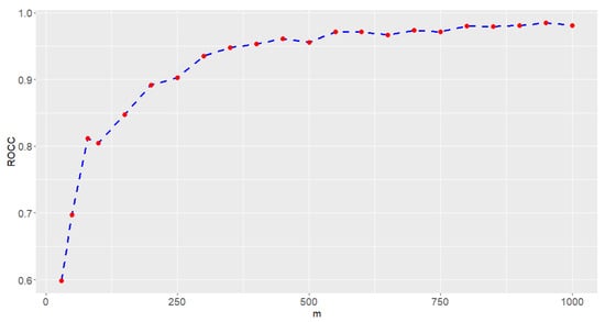
Figure 9.
The ROCC values (red dots) of the SVM-CCPR method for PCB data based on different values of m, and the dashed line is used to connect ROCC values.
5. Concluding Remarks
This study utilizes a method that integrates AIC model selection with machine learning methods to enhance the accuracy and efficiency of CCPR. The novelty lies in combining the model selection with weak learners in machine learning to enhance their ability to control chart pattern recognition. The weak learners, SVM, RF, and KNN, are included in this study to combine the model selection method to develop the SVM-CCPR, RF-CCPR, and KNN-CCPR methods. Simulations show that the SVM-CCPR method outperforms the other two competitors in terms of the recognition rate.
Through simulation and example analysis, the research results indicate that this method can significantly improve recognition accuracy and enhance the classification rate if the distribution of the SPC data is unimodal. The proposed method uses t distribution for the quality variable to develop the proposed CCPR methods. Hence, the proposed SVM-CCPR, RF-CCPR, and KNN-CCPR methods can deal with the symmetric distributions with thin or heavy tails.
Firstly, this study simulates five types of control chart patterns and uses the t distribution with different degrees of freedom and parameter settings to simulate control chart data. After the distribution is identified based on the in-control samples using the AIC criterion, the necessary training data for the CCPR methods are generated to establish the three machine learning models. Simulation results show that the ROCC of recognition by the SVM-CCPR, RF-CCPR, and KNN-CCPR methods gradually increases as the number of charts increases. The findings prove that the SVM-CCPR method can maintain a high level of recognition accuracy over its two competitors.
In the example analysis, data were generated with seven patterns based on a realistic PCB case. Then, the quality of the SVM-CCPR method was evaluated based on different numbers of samples. Though the patterns of the example are different from the simulation study, the SVM-CCPR method can perform well with a high ROCC for pattern recognition. Increasing the number of charts in samples can significantly enhance the value of ROCC. This demonstrates the reliability and stability of the proposed SVM-CCPR method in practical applications. In this stage, it is hard to find pattern recognition examples because most industrial examples are confidential and cannot be released. However, pattern recognition has become increasingly important in quality control applications. Today, Internet of Things (IoT) devices are widely used in manufacturing. Continuously collecting data sets over time is more straightforward than before. Developing simple and efficient CCPR methods is important today.
Integrating model selection with a weak learner can potentially enhance the performance of the weak learner in pattern recognition of process monitoring. In this study, we consider the t distribution to cover the normal distribution as a special case and include heavy-tailed cases for model selection. Skew-t distribution is a generalized case of the t distribution. Hence, skew-t distribution can be another potential candidate for the distribution of error terms. Skew-t distribution can cover asymmetrical data and include the t distribution as a special case. Skew-t distribution has a distribution formula that is more complicated than the t distribution. To obtain reliable parameter estimates of the skew-t distribution for processing monitoring is a challenge. Exploring the application of the proposed CCPR method for the skew-t distribution in control chart recognition can be a future study.
Author Contributions
Conceptualization, investigation, writing, review and editing, and project administration: T.-R.T.; writing: T.-H.W.; validation, investigation, and review and editing: Y.L.; methodology: C.-J.S.; investigation: I.-F.C., C.-J.S. and T.-H.W.; funding acquisition: T.-R.T. All authors have read and agreed to the published version of the manuscript.
Funding
This research was funded by the National Science and Technology Council, Taiwan, grant number NSTC 112-2221-E-032-038-MY2.
Data Availability Statement
The data were generated using the formulas of Case E1 to Case E5 in Section 5 based on the data description in [6].
Conflicts of Interest
The authors declare no conflicts of interest.
References
- Wang, F.K.; Bizuneh, B.; Cheng, X.B. One-sided control chart based on support vector machines with differential evolution algorithm. Qual. Reliab. Eng. Int. 2019, 35, 1634–1645. [Google Scholar] [CrossRef]
- Unlu, R. Cost-oriented LSTM methods for possible expansion of control charting signals. Comput. Ind. Eng. 2021, 154, 107163. [Google Scholar] [CrossRef]
- Lee, P.-H.; Torng, C.-C.; Lin, C.-H.; Chou, C.-Y. Control chart pattern recognition using spectral clustering technique and support vector machine under gamma distribution. Comput. Ind. Eng. 2022, 171, 108437. [Google Scholar] [CrossRef]
- Miao, Z.; Yang, M. Control chart pattern recognition based on convolution neural network. In Smart Innovations in Communication and Computational Sciences: Proceedings of ICSICCS; Springer: Singapore, 2017; Volume 2, pp. 97–104. [Google Scholar]
- Fuqua, D.; Razzaghi, T. A cost-sensitive convolution neural network learning for control chart pattern recognition. Expert Syst. Appl. 2020, 150, 113275. [Google Scholar] [CrossRef]
- Cheng, C.-S.; Ho, Y.; Chiu, T.-C. End-to-end control chart pattern classification using a 1D convolutional neural network and transfer learning. Processes 2021, 9, 1484. [Google Scholar] [CrossRef]
- Cheng, C.-S.; Chen, P.-W.; Ho, Y. Control Chart Concurrent Pattern Classification Using Multi-Label Convolutional Neural Networks. Appl. Sci. 2022, 12, 787. [Google Scholar] [CrossRef]
- Xue, L.; Wu, H.; Zheng, H.; He, Z. Control chart pattern recognition for imbalanced data based on multi-feature fusion using convolutional neural network. Comput. Ind. Eng. 2023, 182, 109410. [Google Scholar] [CrossRef]
- Yu, Y.; Zhang, M. Control chart recognition based on the parallel model of CNN and LSTM with GA optimization. Expert Syst. Appl. 2021, 185, 115689. [Google Scholar] [CrossRef]
- Tian, G.; Liu, Y.; Wang, N.; Liang, X.; Sun, J. A Novel Deep Learning Approach to Online Quality Control for Multiple Time Series Process with Imbalanced Data. Available online: https://ssrn.com/abstract=4633193 (accessed on 20 January 2025).
- Alwan, W.; Ngadiman NH, A.; Hassan, A.; Saufi, S.R.; Mahmood, S. Ensemble classifier for recognition of small variation in x-bar control chart patterns. Machines 2023, 11, 115. [Google Scholar] [CrossRef]
- Sabahno, H.; Niaki, S.T.A. New machine-learning control charts for simultaneous monitoring of multivariate normal process parameters with detection and identification. Mathematics 2023, 11, 3566. [Google Scholar] [CrossRef]
- Yeganeh, A.; Chukhrova, N.; Johannssen, A.; Fotuhi, H. A network surveillance approach using machine learning based control charts. Expert Syst. Appl. 2023, 219, 119660. [Google Scholar] [CrossRef]
- Pham, D.T.; Oztemel, E. Combining multi-layer perceptrons with heuristics for reliable control chart pattern classification. In WIT Transactions on Information and Communication Technologies; WIT Press: Southampton, UK, 2024; Volume 1. [Google Scholar]
- Li, Y.; Dai, W.; He, Y. Control chart pattern recognition under small shifts based on multi-scale weighted ordinal pattern and ensemble classifier. Comput. Ind. Eng. 2024, 189, 109940. [Google Scholar] [CrossRef]
- Zan, T.; Chen, J.; Sun, Z.; Liu, Z.; Wang, M.; Gao, X.; Gao, P. Pattern recognition of control chart with variable chain length based on recurrent neural network. Adv. Manuf. 2024, 1, 0003. [Google Scholar] [CrossRef]
- Ranaee, V.; Ebrahimzadeh, A.; Ghaderi, R. Application of the PSO–SVM model for recognition of control chart patterns. ISA Trans. 2010, 49, 577–586. [Google Scholar] [CrossRef] [PubMed]
- Smola, A.J.; Schölkopf, B.; Müller, K.-R. The connection between regularization operators and support vector kernels. Neural Netw. 1998, 11, 637–649. [Google Scholar] [CrossRef] [PubMed]
- Lu, C.-J.; Shao, Y.E.; Li, C.-C. Recognition of concurrent control chart patterns by integrating ICA and SVM. Appl. Math. Inf. Sci. 2014, 8, 681. [Google Scholar] [CrossRef]
- Montgomery, D.C. Introduction to Statistical Quality Control, 8th ed.; John Wiley & Sons: Hoboken, NJ, USA, 2020. [Google Scholar]

Disclaimer/Publisher’s Note: The statements, opinions and data contained in all publications are solely those of the individual author(s) and contributor(s) and not of MDPI and/or the editor(s). MDPI and/or the editor(s) disclaim responsibility for any injury to people or property resulting from any ideas, methods, instructions or products referred to in the content. |
© 2025 by the authors. Licensee MDPI, Basel, Switzerland. This article is an open access article distributed under the terms and conditions of the Creative Commons Attribution (CC BY) license (https://creativecommons.org/licenses/by/4.0/).