A Unified Control System with Autonomous Collision-Free and Trajectory-Tracking Abilities for Unmanned Surface Vessels Under Effects of Modeling Certainties and Ocean Environmental Disturbances

Abstract

A unified control system that possesses the abilities to arrange collision-free trajectories, precise trajectory tracking, and control allocation for unmanned surface vessels is investigated in this paper by integrating methods, including an image-based trajectory generator, a nonlinear robust controller, and a control allocation maker. For the purpose of rapidly generating an optimal collision-free trajectory, a rapid image-searching method, named double-sided Finite Angle A* (FAA*), is developed to cooperate with a continuous trajectory generator. This proposed control system provides an effective means for letting controlled unmanned surface vessels be able to execute given tasks by following collision-free trajectories under the influences of modeling uncertainties and ocean environmental disturbances. To eliminate the effects of modeling uncertainties and ocean environmental disturbances, a robust compensator is developed to co-work with a nonlinear control law. Furthermore, the required robust control commands are perfectly performed by a pair of rotatable actuators with an analytical control allocation design. Finally, two demonstrations are examined to validate the control performance of this proposed unified control system.

1. Introduction

About 90% of global trade is completed by marine transportation, since seaborne trade offers competitive benefits to shipping companies and consumers. However, the shipping industry has been discomfited by the shortage of crew in recent years. The shipping industry has begun to consider the alternative, and a well-controlled unmanned surface vessel is one of the possible solutions for overcoming this problem. As mentioned above, the usage of unmanned surface vessels can effectively solve the problem of seafarer shortage and decrease expenses. The concept of unmanned surface vehicles (USVs) has been introduced in the last several decades, including Ships, and Shipping of Tomorrow proposed the idea that marine vessels will be navigated with the use of computers in 1973 [1]. The race between major shipbuilding companies and research institutes for autonomous ships is already underway, as the autonomous ships market is predicted to reach USD 235.73 billion by 2028, according to Acute Market Reports [2]. In addition, Hyundai Heavy Industries’ Avikus has built an LNG carrier, the Prism Courage, which is equipped with level-two autonomous navigation technology, that successfully completed the world’s first transoceanic voyage on June 2, 2022 [3]. The Prism Courage sailed roughly 10,000 km with the autonomous control system, almost half the distance of the voyage. From these successful applications, it is obvious that the ability to autonomously plan and track collision-free trajectories in the challenging global ocean environment has become the most important research area for building USVs. After reviewing the existing literature about control designs of USVs, the required functions for constructing the abilities to be collision-free and have trajectory tracking and control allocation in USVs were proposed separately in the past decade. Generally speaking, a completed pilot system of real USVs should integrate a path-planning function, a trajectory-tracking function, and a control allocation design. However, the connection between these three functions is rather weak in the published literature. For example, several papers developed path-planning schemes to search for feasible collision-free paths by using a dynamic window algorithm [4], global–local hybrid [5], A* [6], genetic algorithm [7], fast-marching method [8], etc., without taking control design into consideration, and some of these collision-free trajectory-searching methods are not able to generate collision-free trajectory patterns in real-time. As to control designs of USVs, waypoint tracking control designs have served an important function in the past decades, including line-of-sight (LOS) control designs [9,10], point-to-point navigation [11], and nonlinear optimal control [12]. Control laws developed for USVs based on the LOS tracking concept inevitably have a high gain property, and the power consumption is naturally high. For easing this high gain property, control designs, such as singular perturbation control design [13] and nonlinear robust control design [14], are proposed to perform control actions, in order to lead USVs to track standard test paths, including straight, ramp, parabolic, and specific trajectories, as closely as possible recently. It is a pity that collision-free trajectory-planning schemes are never simultaneously considered for practical applications in USVs. In addition, control allocation methodology for how to generate desired control commands with installed actuators, such as rotatable waterjets, outboard motors, etc., should be developed for practical control designs in USVs as well. Recently, several existing pieces of literature discussed actuators’ fault problems in nonlinear systems based on an adaptive fuzzy control algorithm and an adaptive fuzzy output feedback control algorithm [15,16,17,18]. These kinds of advanced fault-tolerant control designs would be great for mature USV systems at some point in the future. At the present stage, a control allocation method that can precisely distribute the desired control commands to the outputs of actuators is an urgent need to address. To overcome the drawbacks of these investigations, a unified control system that combines three major functions, including 1. path planning methodology, 2. nonlinear robust control design, and 3. the control allocation method, is proposed for the collision-free and trajectory-tracking problems in USVs. In this investigation, a new multi-side searching method, which can greatly decrease searching time, is developed for generating collision-free trajectories for USVs from interesting regions in images. Then, a nonlinear robust control law is designed to mitigate the effects of modeling uncertainties and ocean disturbances, such as winds, currents, and waves. For meeting the practical implementation of guiding USVs with actuators to follow arbitrary given trajectories, a control allocation method is proposed to convert the desired robust control commands into the outputs of installed actuators.

This investigation is organized as follows. Descriptions of the proposed unified control system are comprehensively introduced in Section 2. A collision-free trajectory generator is described by addressing waypoint generation and path smoothing in Section 3. In Section 4, the proposed nonlinear robust control scheme is developed. Control allocation methodology for a controlled USV with two rotatable actuators is derived in Section 5. The control performance of this proposed unified control system for USVs in real-world geographies is conducted in Section 6. The conclusions are summarized in Section 7.

2. Unified Control System for Unmanned Surface Vessels

As shown in Figure 1, this proposed unified control system for USVs mainly consists of four parts for achieving collision-free and precise trajectory-tracking performance under the effects of modeling uncertainties and ocean disturbances. The methods involved in this unified control system are 1. an information acquisition method, 2. a collision-free trajectory generator, 3. a nonlinear robust control law, and 4. an analytical control allocation.

In this investigation, we assume that images of interested areas can be obtained in real-time from the satellite during the phase of information acquisition. Then, satellite images of the interested regions where the controlled USV executes tasks are downloaded for the purpose of generating a collision-free trajectory. For generating a collision-free trajectory, a collision-free trajectory generator, which combines a rapid FAA* algorithm and a trajectory interpolator, is developed for this phase. In the third phase, a nonlinear robust control law is investigated for overcoming the influences of ocean environmental disturbances and modeling uncertainties. Furthermore, the required robust control command in the third phase will be analytically transformed into rotatable angles and control forces of the installed actuators for the rudders, outboard propellers, waterjets, etc., in the final phase. Details of the above-mentioned methods will be introduced subsequently.

3. Design of the Collision-Free Trajectory Generator

In the first phase, the real-time image, which is demanded for executing given missions, as shown in Figure 2, can be captured and transmitted to the controlled USV. Figure 2 will be adopted as a test bay for verifying the performance of this proposed unified control system, and this image shows Yongxin Harbor (Kaohsiung, Taiwan) and the surrounding areas.

After receiving the transmitted image, a rapid collision-free trajectory generator algorithm will be utilized to plan a collision-free trajectory. The collision-free trajectory generator is constructed by a rapid FAA* method for searching collision-free waypoints, and a continuous trajectory interpolator is then used to interpolate these collision-free waypoints and generate continuous trajectories.

3.1. Rapid Collision-Free Trajectory Generator

This trajectory generator consists of three parts: 1. edge detection of the captured image, 2. indication of collision-free waypoints, and 3. continuous trajectory generation. For the first part, two image operations are adopted in this paper, which are binarization and morphology. The usage of these two image operations to capture images is described below.

3.1.1. Edge Detection and Geofencing Construction

Otsu’s method is applied to automatically perform thresholds for separating the pixels of the transmitted images into two categories: 1. dark pixels for ocean and river and 2. white pixels for static obstacles, such as banks, buildings, and so on. Applying Otsu’s method to Figure 2, the binarization result of the image process is shown in Figure 3.

In addition, to create a safe geofencing for the controlled USV to avoid being too close to static objects, the most famous morphological operation, namely dilation, is applied, since it can thicken the outer edges of obstacles in the received images.

As Figure 4, the image dilation operation applies a structuring element to the received image. Then, a same-sized output image is created. This output image’s pixel value is calculated based on comparisons of the same pixel in the received image with its neighbors. The following is a sample description of the dilation image process.

With the input of a binary image I and the structuring element D, the dilation of $I$ by $D$ is denoted $I\oplus D$, as in:

$$I\oplus D=\left\{\left.z\right|D_z\cap I\ne ⌀\right\}$$

(1)

where $D_z=\left\{\left.z+d\right|d\in D\right\}$ represents the sets of pixels after the structuring element acted and is shifted by z. d is the coordinate index of D. In the following, an origional binary image (left) and a structuring element (right) in Figure 4 is adopted to demostrate the dilation image process.

Figure 5 reveals the output image after using the dilation operation, and the boundary (pink color) of this operation becomes the geofencing for the controlled USV to avoid collisions with static obstacles.

In this investigation, a square structuring element is chosen. The adopted structuring element D is expressed as a function of the length of ship L, the line of sight $\sqrt{2}/2$, and the adjustable weight of dilation w:

$$dimensio{n}_D=2\times \left[L\times \sqrt{2}\right]+w$$

(2)

The selection for w has a criterion based on the profile of obstacles in the received image: “the obstacle is with thin lines, and one can increase the value of w to make sure the obstacle is all contained”. With this margin design for a received image, the geofencing will provide more tolerance for the controlled USV, protecting it from collisions. The dilation result of Figure 2 is displayed in Figure 6.

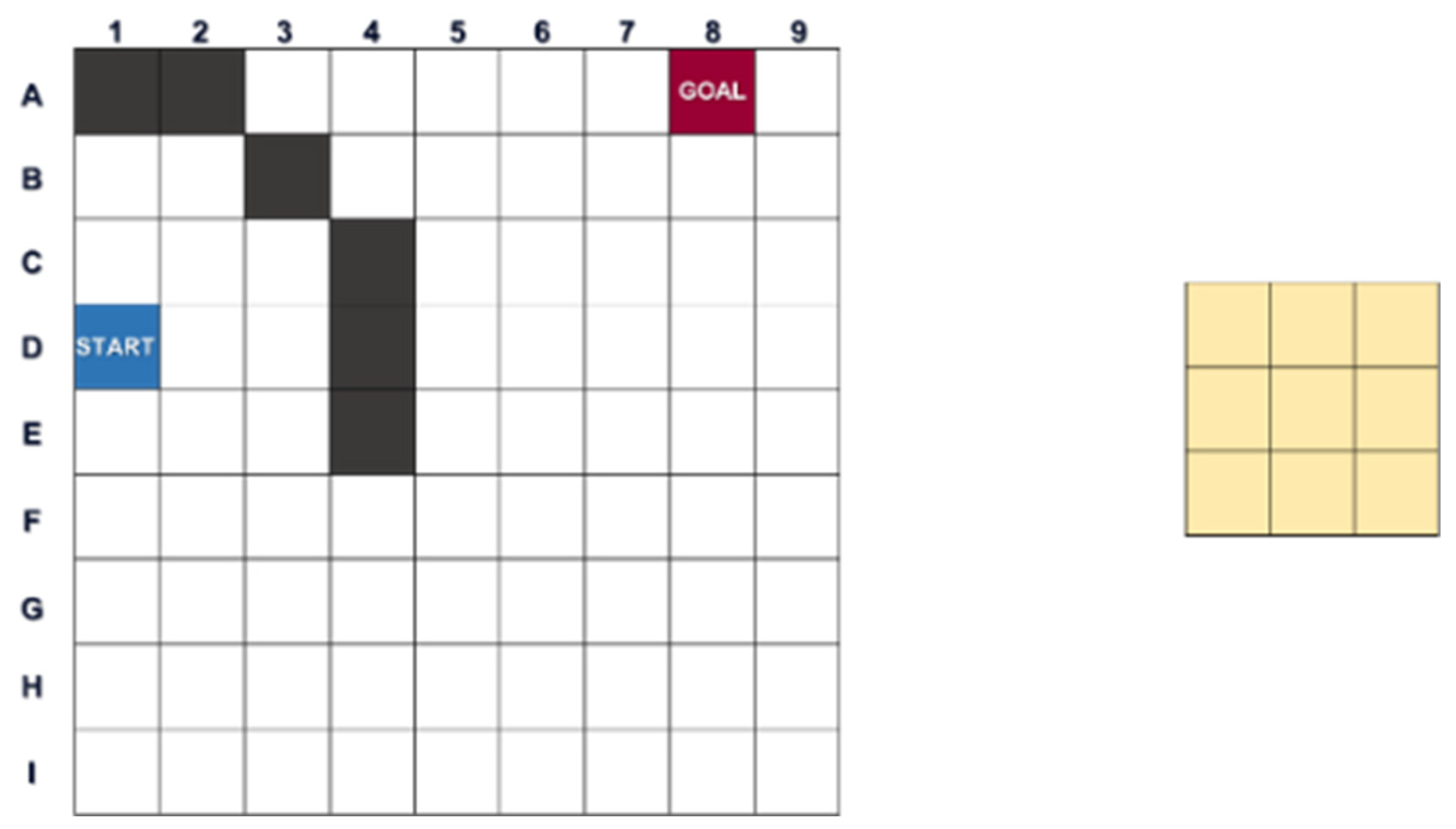
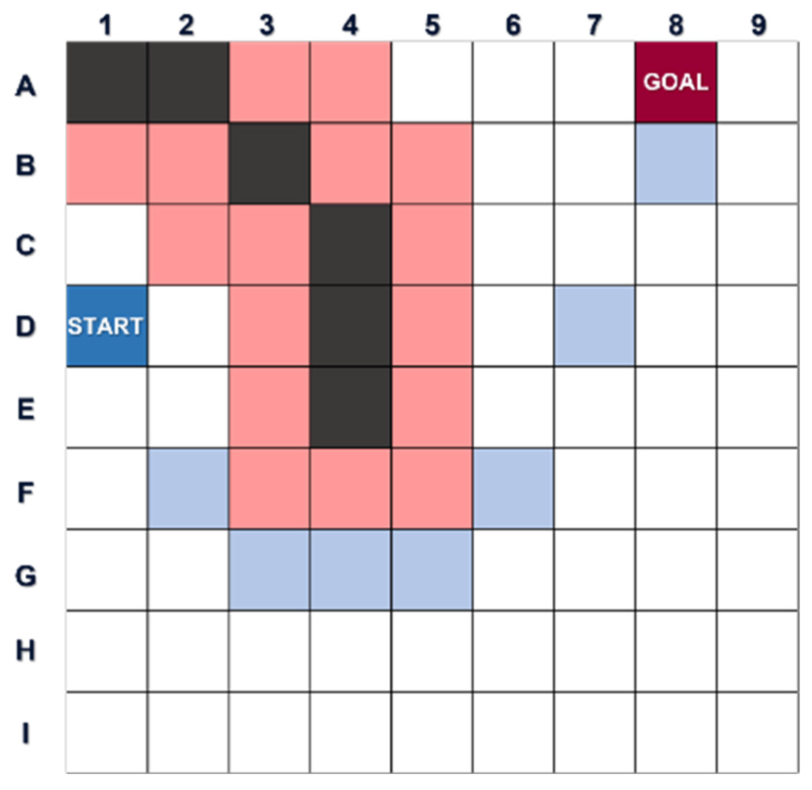
3.1.2. Collision-Free Waypoint-Searching Method with a Multi-Sided Finite Angle A* (FAA*) Algorithm

After identifying the contours of all obstacles and delivering the geofencing for the interested areas, as in the examples of Figure 2, Figure 3 and Figure 6, a multi-sided FAA* algorithm will be then utilized to search for the best collision-free points of the interested areas that have no collision risks. After deploying the above contour identification method for static obstacles in received images, an effective searching method should be adopted for finding a set of collision-free waypoints. The FAA* algorithm is one of the most common graph traversals and path-search algorithms in many fields, such as shortest-path finding for computer games or path planning for robots [19]. For decreasing collision-free waypoint searching speed, one multi-sided FAA* algorithm which is the improved version of the FAA* algorithm and is capable of reducing the computation complexity and computation time by equally cutting the total sailing path from the start point and goal point is proposed. Based on this new methodology, the computation time spent on searching for collision-free waypoints can be greatly decreased. The following is an example adopted for demonstrating this proposed double-sided FAA* algorithm. The following simulation results are collision-free trajectories, as shown in Figure 7 and Figure 8, from the start point (blue circle) to the goal (black point) of a complex map based on a single-sided FAA* and a double-sided FAA* algorithm, respectively. An approximate middle point is made first on this map (the intersection of the blue line and the red line of Figure 8). Then, the proposed double-sided FAA* method searches for a collision-free trajectory from the start point to the goal simultaneously. Finally, a collision-free trajectory that integrates the blue line and the red line is displayed in Figure 8. The run times of the single-sided FAA* algorithm and the double-sided FAA* algorithm while searching for this collision-free trajectory are 0.81 s and 0.43 s, respectively.

The result illustrating the combination of geofencing and the double-sided FAA* algorithm is revealed in Figure 9. In Figure 9, a layer of geofencing (pink color) is made for covering the outer edges of obstacles, and a set of collision free waypoints (blue points) are found optimally.

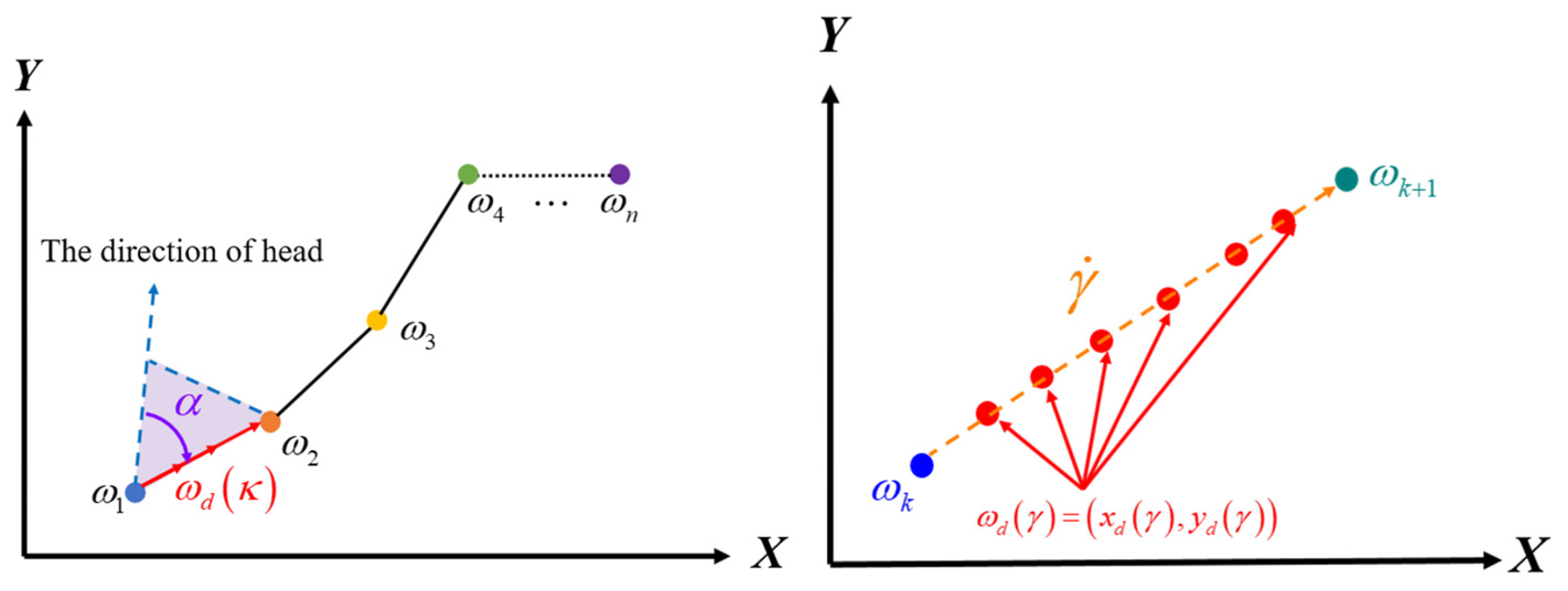
3.1.3. Continuous Trajectory Generator

Intuitively, straightly connecting all collision-free waypoints in Figure 9 to obtain a desired continuous collision-free trajectory is reasonable. However, the collision-free trajectory is the blue continuous trajectory, and several sharp turning angles for the controlled USV to perform will be generated.

To overcome the drawback of generating sharp turning angles, as shown in Figure 10, in this investigation, an interpolation algorithm, as below, is developed to connect all of the collision-free waypoints and generate a smooth trajectory for the controlled USV. As mentioned above, by straightly connecting all collision-free waypoints (pixels of received images) to plan a collision-free path with the proposed multi-sided FAA* algorithm, dense collision-free waypoints will be obtained, and the computation efforts extremely increase once ultra-high-density images are used. Diluting dense waypoints into reasonable amounts becomes the major task before connecting them. The following condition is proposed for easing this situation.

Condition 1.

A criterion for diluting dense collision free waypoints is indicated as Equation (3):

$$\left|{\omega }_k-{\omega }_{k+1}\right|>kL$$

(3)

where w_n is the current point, w_n+1 is the next point, k is an adjustable parameter that can be selected based on the controlled USV’s sailing speed, and L is the length of the controlled USV.

Based on Condition 1, a set of identified collision-free waypoints ${\omega }_k={\left[\begin{array}{cc}{x}_k& y_k\end{array}\right]}^T\in {ℝ}^2,k=1,2,\dots ,n$, diluting from the set of waypoints selected by multi-sided FAA* algorithm, can be obtained for constructing a continuous and smooth trajectory.

3.1.4. Continuous and Smooth Trajectory Generator

To prevent the controlled USVs from collisions with obstacles and sudden changes in sails in complex ocean environments, it is vital to develop a trajectory generator to plan collision-free and smooth trajectories to enable collision-free actions for controlled USVs. By employing interpolation, a set of identified collision-free waypoints ${\omega }_k={\left[\begin{array}{cc}{x}_k& y_k\end{array}\right]}^T\in {ℝ}^2,k=1,2,\dots ,n$ based on a multi-sided FAA* algorithm can be interpolated to form a smooth trajectory, as in Figure 11. The way to plan the desired trajectory using collision-free waypoints is expressed below:

$$\begin{array}{l}{X}_d(\gamma )=x_k+\gamma \cos \alpha \\ Y_d(\gamma )=y_k+\gamma \sin \alpha \end{array}$$

(4)

where γ is the trajectory parameter, and α is the heading angle of the desired trajectory, presented as follows:

$$\alpha ={\tan }^{-1}({\displaystyle \frac{\Delta y_k}{\Delta x_k}})$$

(5)

where $\Delta x_k=x_{k+1}-x_k$ and $\Delta y_k=y_{k+1}-y_k$. With the variation of γ, the speed of the USV will also be controlled to the desired speed $U_d$.

$$\dot{\gamma }(t)={\displaystyle \frac{U_d}{\sqrt{{X_d^{\prime }}^2(\kappa )+{Y_d^{\prime }}^2(\kappa )}}}$$

(6)

Through Equations (4)–(6), collision-free trajectories can be planned, and by using the line of sight (LOS) between the position of the USV and the desired position, the desired yaw angle ${\psi }_d$ can be obtained:

$${\psi }_d={\tan }^{-1}\left({\displaystyle \frac{\left(Y_d-y\right)}{\left(X_d-x\right)}}\right)$$

(7)

The expected tracking trajectory point is denoted as ${\eta }_d={\left[\begin{array}{ccc}{X}_d& Y_d& {\psi }_d\end{array}\right]}^T$. When ${\psi }_d-\psi \to 0$, it signifies that the USV and instantaneous waypoint are in a head-on collision state, and when the tracking error is zero, the USV will pass through each collision-free waypoint.

Figure 12 shows the comparisons of the search result of the multi-sided FAA* algorithm via directly connecting two neighboring waypoints (green color) and the trajectory (red color) interpolated by the proposed collision-free control system. This figure reveals that the green trajectory consists of several sharp turning points, and they are difficult for the controlled USVs to follow up on based on the limited command outputs of installed actuators. By utilizing this proposed interpolation algorithm, a smooth collision-free trajectory can be obtained, such as the trajectory in Figure 12 plotted in a red color.

4. Nonlinear Robust Control Law Design for USVs with Modeling Uncertainties and Ocean Disturbances

The underactuated dynamics of the controlled USV are formulated below [14]:

$$M_E(\eta )\ddot{\eta }+C_E(B,\eta )\dot{\eta }+D_E(\eta )\dot{\eta }={\tau }_E+{\tau }_{dE}$$

(8)

where $\eta ={[X,Y,\psi ]}^T$ is the state vector of the controlled USV in the Earth frame, and $B={\left[u,v,r\right]}^T$ stands for the linear velocities of the controlled USV in the body frame. The system parameter matrices, including $M_E(\eta )$, $C_E(B,\eta )$ and $D_E(\eta )$, are the inertia mass matrix, the Coriolis and centripetal matrix, and the damping matrix. ${\tau }_E={\left[\begin{array}{ccc}{F}_X& F_Y& M_Z\end{array}\right]}^T$ is the control command, and ${\tau }_{dE}$ involves the ocean’s environmental disturbances coming from random waves, winds, and currents in the Earth frame, respectively.

From a real implementation point of view, the system parameter matrices should be presented as a perturbed formulation, as follows:

$$M_E(\eta )={\overline{M}}_E(\eta )+\Delta M_E(\eta )$$

(9a)

$$C_E(B,\eta )={\overline{C}}_E(B,\eta )+\Delta C_E(B,\eta )$$

(9b)

$$D_E(\eta )={\overline{D}}_E(\eta )+\Delta D_E(\eta )$$

(9c)

where ${\overline{M}}_E(\eta )$, ${\overline{C}}_E(B,\eta )$, and ${\overline{D}}_E(\eta )$ are the nominal terms, and $\Delta M_E(\eta )$, $\Delta C_E(B,\eta )$, and $\Delta D_E(\eta )$ are the modeling uncertainties. The modeling uncertainties strongly affect the control performance since most nonlinear-based control designs depend on the accurate dynamics of controlled USVs, except for traditional linear control designs, such as PID control designs. However, it is impossible to obtain 100% accurate dynamics for the controlled USV, even with the help of towing tank experiments. Hence, an extra control mean should be considered to eliminate the effects of modeling uncertainties.

Substituting Equation (9a–c) into Equation (8), the dynamics of the controlled USV can be further expressed as:

$${\overline{M}}_E(\eta )\ddot{\eta }+{\overline{C}}_E(B,\eta )\dot{\eta }+{\overline{D}}_E(\eta )\dot{\eta }={\tau }_E+{\tau }_{dEA}$$

(10)

where ${\tau }_{dEA}=\Delta M_E(\eta )\ddot{\eta }+\Delta C_E(B,\eta )\dot{\eta }+\Delta D_E(\eta )\dot{\eta }+{\tau }_{dE}$ is the combination of disturbances and modeling uncertainties.

Define the trajectory-tracking error vector e between the controlled USV (η) and the desired trajectory (η_d) as:

$$e=\eta -{\eta }_d$$

(11)

where $e={\left[\begin{array}{ccc}{e}_x& e_y& e_{\psi }\end{array}\right]}^T$, $\eta ={\left[\begin{array}{ccc}X& Y& \psi \end{array}\right]}^T$, and ${\eta }_d={\left[\begin{array}{ccc}{X}_d& Y_d& {\psi }_d\end{array}\right]}^T$.

Assumption 1.

The desired trajectory is supposed to be known, smooth, bounded and at least second time derivative η_d ∈ C^∞ [16].

A trajectory-tracking error dynamics can be derived for presenting the closed-loop behavior between the controlled USV and the desired trajectory as:

$$\begin{array}{cc}\hfill \ddot{e}& =\ddot{\eta }-{\ddot{\eta }}_d\hfill \\ & =-{\overline{M}}_E{(\eta )}^{-1}({\overline{C}}_E(B,\eta )+{\overline{D}}_E(\eta ))\dot{\eta }\hfill \\ & +{\overline{M}}_E{(\eta )}^{-1}{\tau }_E+{\overline{M}}_E{(\eta )}^{-1}{\tau }_{dEA}-{\ddot{\eta }}_d\hfill \end{array}$$

(12)

Select a nonlinear robust control law τ_E as follows:

$${\tau }_E={\overline{M}}_E(\eta )\left\{{\overline{M}}_E{(\eta )}^{-1}({\overline{C}}_E(B,\eta )+{\overline{D}}_E(\eta ))\dot{\eta }+V+{\ddot{\eta }}_d+{\Delta }_c\right\}$$

(13)

where $V={\left[{\mathrm{V}}_1{ \mathrm{V}}_2{ \mathrm{V}}_3\right]}^T$ is

$${\mathrm{V}}_1={\ddot{X}}_d+{\sigma }_{P1}(X-X_d)+{\sigma }_{I1}{\displaystyle {\int }_{t_0}^{t_f}(X-X_d)}dt+{\sigma }_{D1}(\dot{X}-{\dot{X}}_d)$$

(14)

$${\mathrm{V}}_2={\ddot{Y}}_d+{\sigma }_{P2}(Y-Y_d)+{\sigma }_{I1}{\displaystyle {\int }_{t_0}^{t_f}(Y-Y_d)}dt+{\sigma }_{D2}(\dot{Y}-{\dot{Y}}_d)$$

(15)

$${\mathrm{V}}_3={\ddot{\psi }}_d+{\sigma }_{P3}(\psi -{\psi }_d)+{\sigma }_{I3}{\displaystyle {\int }_{t_0}^{t_f}(\psi -{\psi }_d)}dt+{\sigma }_{D3}(\dot{\psi }-{\dot{\psi }}_d)$$

(16)

and the control parameters ${\sigma }_{Pi}$, ${\sigma }_{Ii}$, and ${\sigma }_{Di}$, for i = 1, 2, 3 are artificially designable values. As to the design of the robust eliminator, Δ_c will be developed in the subsequent section.

Substituting nonlinear robust control law τ_E in Equation (13) into Equation (12), a perturbed second-order trajectory-tracking error dynamics is yielded, as below:

$$\ddot{e}+K_D\dot{e}+K_{P}e+K_I{\displaystyle {\int }_{t_0}^{t_f}edt}={\Delta }_c+W$$

(17)

$$K_P=\left[\begin{array}{ccc}{\sigma }_{P1}& 0& 0\\ 0& {\sigma }_{P2}& 0\\ 0& 0& {\sigma }_{P3}\end{array}\right], K_I=\left[\begin{array}{ccc}{\sigma }_{I1}& 0& 0\\ 0& {\sigma }_{I2}& 0\\ 0& 0& {\sigma }_{I3}\end{array}\right], K_D=\left[\begin{array}{ccc}{\sigma }_{D1}& 0& 0\\ 0& {\sigma }_{D2}& 0\\ 0& 0& {\sigma }_{D3}\end{array}\right],$$

and $W={\overline{M}}_E{(\eta )}^{-1}{\tau }_{dEA}$.

Robust Eliminator Design

Since disturbances W persistently import the trajectory-tracking error dynamics in Equation (17), the convergence $\underset{t\to \infty }{\lim }e(t)=0$ of the trajectory-tracking error e in Equation (11) or Equation (12) cannot be ensured. Even the Hurwitz condition in Equation (17) is satisfied by selecting a set of control parameters (${\sigma }_{Pi}$, ${\sigma }_{Ii}$ and ${\sigma }_{Di}$). To guarantee the robust property of the trajectory-tracking errors e and the robust compensator Δ_c with respect to disturbances W, the detailed proof and robust design procedure will be derived in this following analysis.

Rewriting Equation (17) as an augmented form, we have:

$$\dot{E}=AE+B{\Delta }_c+BW$$

(18)

$$E={\left[\begin{array}{ccccccccc}{e}_x& {\displaystyle {\int }_0^{t_0}{e}_{x}dt}& {\dot{e}}_x& e_y& {\displaystyle {\int }_0^{t_0}{e}_{y}dt}& {\dot{e}}_y& e_{\psi }& {\displaystyle {\int }_0^{t_0}{e}_{\psi }dt}& {\dot{e}}_{\psi }\end{array}\right]}^T,$$

$$\begin{gathered} A=\left[\begin{array}{ccc}{A}_{11}& 0_{3\times 3}& 0_{3\times 3}\\ 0& A_{22}& 0_{3\times 3}\\ 0_{3\times 3}& 0_{3\times 3}& A_{33}\end{array}\right], A_{11}=\left[\begin{array}{ccc}0& 1& 0\\ 1& 0& 0\\ -{\sigma }_{P1}& -{\sigma }_{I1}& -{\sigma }_{D1}\end{array}\right], \\ {A}_{22}=\left[\begin{array}{ccc}0& 1& 0\\ 1& 0& 0\\ -{\sigma }_{P2}& -{\sigma }_{I2}& -{\sigma }_{D2}\end{array}\right], A_{33}=\left[\begin{array}{ccc}0& 1& 0\\ 1& 0& 0\\ -{\sigma }_{P3}& -{\sigma }_{I3}& -{\sigma }_{D3}\end{array}\right] \\ B={\left[\begin{array}{ccccccccc}0& 0& 1& 0& 0& 0& 0& 0& 0\\ 0& 0& 0& 0& 0& 1& 0& 0& 0\\ 0& 0& 0& 0& 0& 0& 0& 0& 1\end{array}\right]}^T \end{gathered}$$

Remark 1.

Each control parameter of the set of control parameters (${\sigma }_{Pi}$, ${\sigma }_{Ii}$, and ${\sigma }_{Di}$) plays a specific role in the overall control performance of this proposed unified control system, and the following are the guidelines for adjusting control parameters: ${\sigma }_{Pi}$, ${\sigma }_{Ii}$ , and ${\sigma }_{Di}$

• adjusting ${\sigma }_{Pi}$ and ${\sigma }_{Ii}$ can decrease the tracking errors in a steady state period;
• adjusting ${\sigma }_{Di}$ can speed up the transient response and quickly converge tracking errors.

Based on the trajectory-tracking error dynamics in Equation (18), the aim of this trajectory-tracking problem of the controlled USV becomes to specify the robust compensator Δ_c for the trajectory-tracking error dynamics in Equation (18) to guarantee that the worst effect of W on trajectory-tracking error E and robust eliminator Δ_c is maintained below a predefined attenuation level $\gamma$ for all t_f ∈ [0,∞) [14]:

$$\underset{{\Delta }_c}{\min }\underset{W}{\max }{\displaystyle \frac{{\displaystyle {\int }_{ 0}^{ t_f}\left[E^{T}QE+{\Delta }_c^{T}R{\Delta }_c\right]dt}}{{\displaystyle {\int }_{ 0}^{ t_f}\left[W^{T}W\right]dt}}}\le {\gamma }^2$$

(19)

where the weighting matrix $Q=Q^T$ and $R=R^T$ are positive definite matrices.

Theorem 1.

The collision-free and trajectory-tracking problem of USVs, considering the effects of modeling uncertainties and ocean environmental disturbances, is resolved by the proposed robust control law ${\tau }_E$, which cooperates with a smooth trajectory generator and a robust compensator as:

$${\tau }_E={\overline{M}}_E(\eta )\left\{{\overline{M}}_E{(\eta )}^{-1}({\overline{C}}_E(B,\eta )+{\overline{D}}_E(\eta ))\dot{\eta }+V+{\ddot{\eta }}_d+{\Delta }_c\right\}$$

(20)

$${\Delta }_c=-R^{-1}{B}^{T}PE$$

where $P=P^T>0$ can be obtained by solving the equation below:

$$PA+A^{T}P+PB\left({\displaystyle \frac{1}{{\gamma }^2}}I-R^{-1}\right)B^{T}P+Q=0$$

(21)

Proof of Theorem 1.

It is given in Appendix A. □

Remark 2.

For this unified control system design problem of USVs, the inputs of the closed-loop system of USVs are the proposed robust control law τ_E and the ocean’s environmental disturbances τ_dE that come from random waves, winds, and currents. Meanwhile, the output of this closed-loop system is the trajectory-tracking error E. From the mathematical derivation of Theorem 1, it is easy to find out the fact that, by using the proposed robust control law τ_E in Equation (20), and considering the worst effect of W, which combines the ocean-environmental disturbances and modeling uncertainties as inputs, the ratio between the inputs (τ_E and W) and the output (E) are bounded below γ². Hence, the whole closed-loop system of the controlled USV must be at least BIBO stable and simultaneously satisfy the robust control performance.

5. Control Allocation Methodology for Installed Actuators

In practice, the above developed control law should be further well-distributed to all installed actuators, such as waterjets, rudders, outboard motors, rudders, etc. The actuators used in the USVs of this investigation are two rotatable waterjets. Hence, in the following, a control allocation design will be proposed based on this configuration.

5.1. Configuration and Input–Output Model of Actuators

In this section, an effective control allocation method will be derived to distribute the desired control law τ_E to the installed rotatable actuators of the controlled USV. Due to the rotatable property, the thrust vectors can be expressed as functions of azimuth angles α_i, for i = 1, 2. It is evident that utilizing rotatable actuators to construct the desired control law τ_E let this control distribution problem become a nonlinear problem with respect to azimuth angles α_i, for i = 1, 2, and the real-time solution of this problem is difficult to solve without using a high-speed calculator. To tackle this issue, the outputs of rotatable waterjets should be treated as two separate forces, and the mathematical relationship is presented as follows:

$${\tau }_{\mathrm{E}}=Tf$$

(22)

where

$${\tau }_{\mathrm{E}}=\left[\begin{array}{c}{F}_x\\ F_y\\ M_z\end{array}\right], T=\left[\begin{array}{cccc}1& 0& 1& 0\\ 0& 1& 0& 1\\ -d_{y_1}& d_{x_1}& -d_{y_2}& d_{x_2}\end{array}\right], f=\left[\begin{array}{c}{F}_{x1}\\ F_{y1}\\ F_{x2}\\ F_{y2}\end{array}\right]$$

where $d_{y_1}$, $d_{y_2}$, $d_{x_1}$, and $d_{x_2}$ are the distances from each waterjet to the center of gravity of the controlled USV. $F_{xi}$ and $F_{yi}$, for i = 1, 2, represent the forces generated in the x and y directions by individual waterjets. The matrix T represents the augmented thrust configuration matrix of the actuators, which describes how the output commands of thrust vector f contribute to the dynamics of the controlled USV. The related azimuth angles, α_i, for i = 1, 2, can be calculated by

$${\alpha }_i={\tan }^{-1}{\displaystyle \frac{F_{y_i}}{F_{x_i}}}$$

(23)

5.2. Optimization for Actuators’ Output Commands

The objective of the control allocation design is to perfectly distribute the proposed nonlinear robust control command τ_E to the output command $\mathbf{f}$ of the rotatable waterjets while minimizing the overall energy consumption of the waterjets. The control allocation problem of the controlled USV can be then formulated as the following constraint problem:

$$\begin{array}{l}\underset{\mathbf{f}}{\min }\left\{{\mathbf{f}}^T{\mathbf{P}}_a\mathbf{f}\right\}\\ s.t.{\mathbf{\tau }}_{\mathrm{E}}-\mathbf{T}\mathbf{f}=0\end{array}$$

(24)

where P_a is the weighting matrix for the power consumption performance index and is a positive definite.

Since this is a constrained least-squares optimization problem, it can be solved by using the method of a Lagrange multiplier. The corresponding Lagrangian can be defined as follows:

$$L(\mathbf{f},\mathbf{\lambda })={\mathbf{f}}^T{\mathbf{P}}_a\mathbf{f}+{\mathbf{\lambda }}^T({\mathbf{\tau }}_{\mathrm{E}}-\mathbf{T}\mathbf{f})$$

(25)

where λ is a vector of Lagrange multipliers introduced to convert the constrained problem into an unconstrained problem. By differentiating Equation (25) with respect to f and λ, the following expressions can be obtained:

$${\displaystyle \frac{\partial L}{\partial \mathbf{f}}}=2{\mathbf{P}}_a\mathbf{f}-{\mathbf{T}}^T\mathbf{\lambda }$$

(26)

$${\displaystyle \frac{\partial L}{\partial \mathbf{\lambda }}}={\mathbf{>\tau }}_{\mathrm{E}}-\mathbf{T}\mathbf{f}$$

(27)

From Equation (26), it results in

$$\mathbf{f}={\displaystyle \frac{1}{2}}{\mathbf{P}}_a^{-1}{\mathbf{T}}^T\mathbf{\lambda }$$

(28)

From Equations (27) and (28), they give the following result:

$${\tau }_{\mathrm{E}}={\displaystyle \frac{1}{2}}{\mathbf{T}}^{-1}{\mathbf{P}}_a{\mathbf{T}}^T\mathbf{\lambda }$$

(29)

The Lagrange multiplier λ can be derived from Equation (29)

$$\mathbf{\lambda }=2{\left({\mathbf{T}}^T{\mathbf{P}}_a^{-1}\mathbf{T}\right)}^{-1}{\tau }_{\mathrm{E}}$$

(30)

Substituting Equation (30) into Equation (28), the optimal thruster output command f* is solved as follows:

$${\mathbf{f}}^{*}={\mathbf{P}}^{-1}{\mathbf{T}}^T{({\mathbf{T}}^T{\mathbf{P}}_a^{-1}\mathbf{T})}^{-1}{\tau }_{\mathrm{E}}$$

(31)

6. Performance Validation of the Proposed Unified Control System

6.1. System Parameters of the Controlled USV

As revealed in Figure 13, system parameters of the controlled USV, which are measured by a real ship-towing experiment, are stated in

Table 1. System parameters of the controlled USV.

Length L	1.72 m
Width B	0.4 m
Draft T	0.3 m
Mass m	41 kg
Iz	6.522 kg∙m
xg	0 m
$X_{\dot{u}}$	−1.291 kg
$Y_{\dot{v}}$	−40.326 kg
$Y_{\dot{r}}$	−39.04525 N∙s2/m2
$N_{\dot{r}}$	200.79808 N∙m∙s
$X_u$	−0.98 N∙s2/m2
$Y_v$	−38.808 N∙s2/m2
$Y_r$	−16.43778 N∙s
$N_v$	−14.340 N∙s2/m2
$N_r$	−236.5 N∙m∙s

[14], and the parameters of the installed actuators are listed in

Table 2. Parameters of the installed actuator.

Thrust force of single waterjet	400 N
Rotatable angle	±120°

. The modeling uncertainties of the controlled USV in practice are considered as 10% random variations of these system parameters, and the ocean environmental disturbance τ_dE is adopted from [14].

Remark 3.

According to the size of the USV adopted in this investigation, the disturbance limitation of the controlled USV, which can prevent keeling over and maintain stability, is ≤sea state 2.

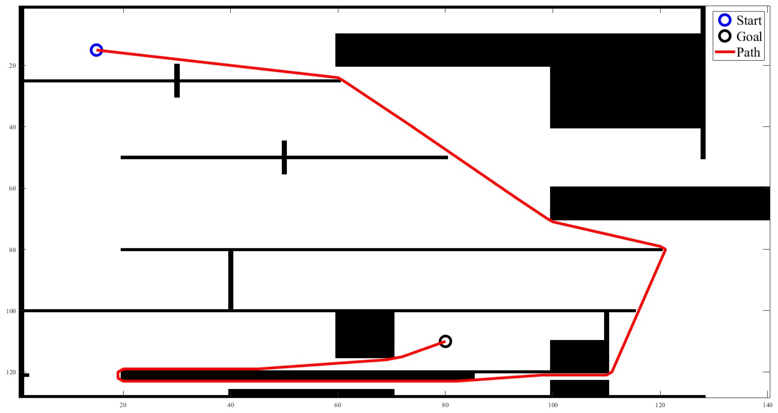
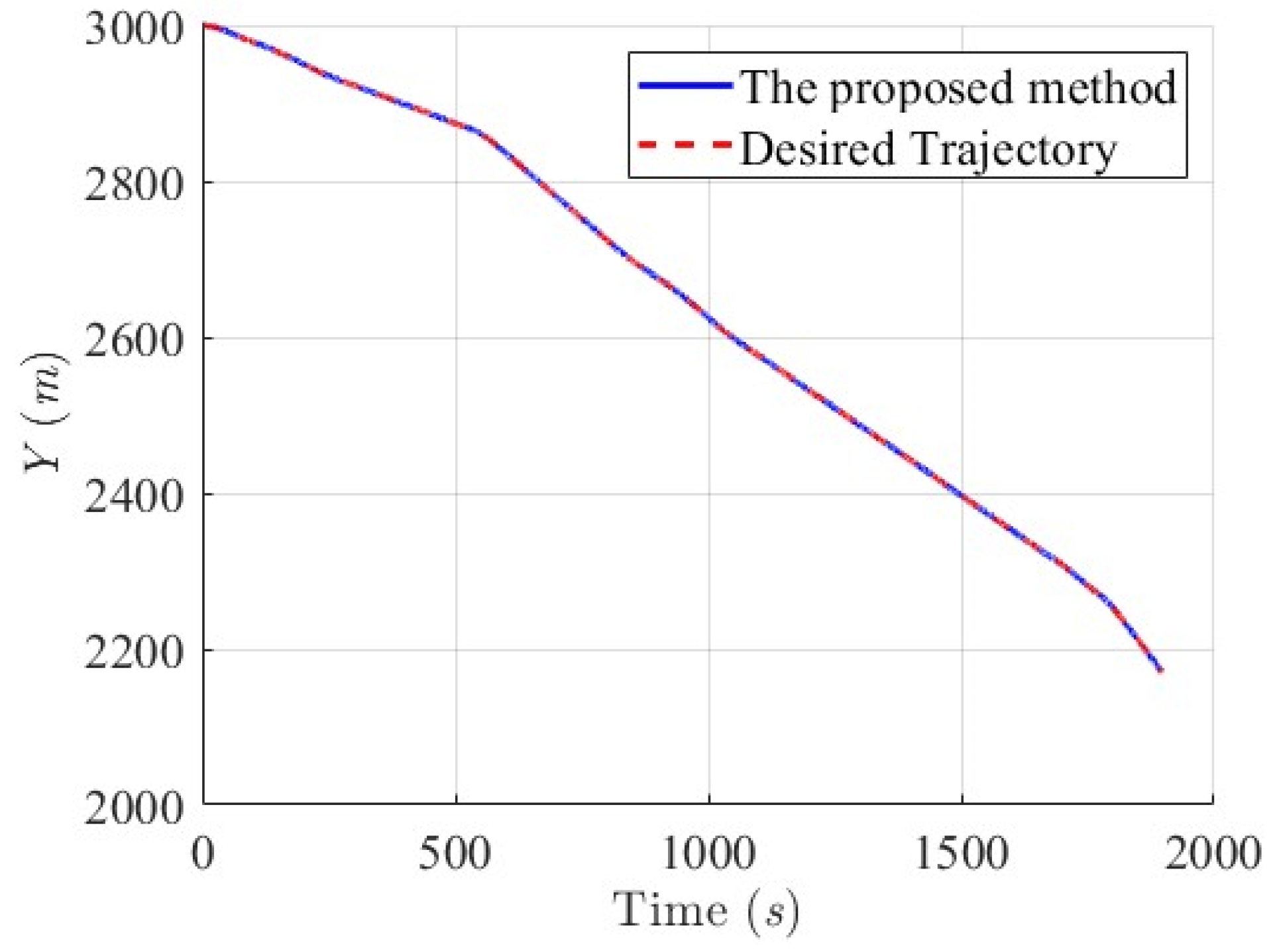
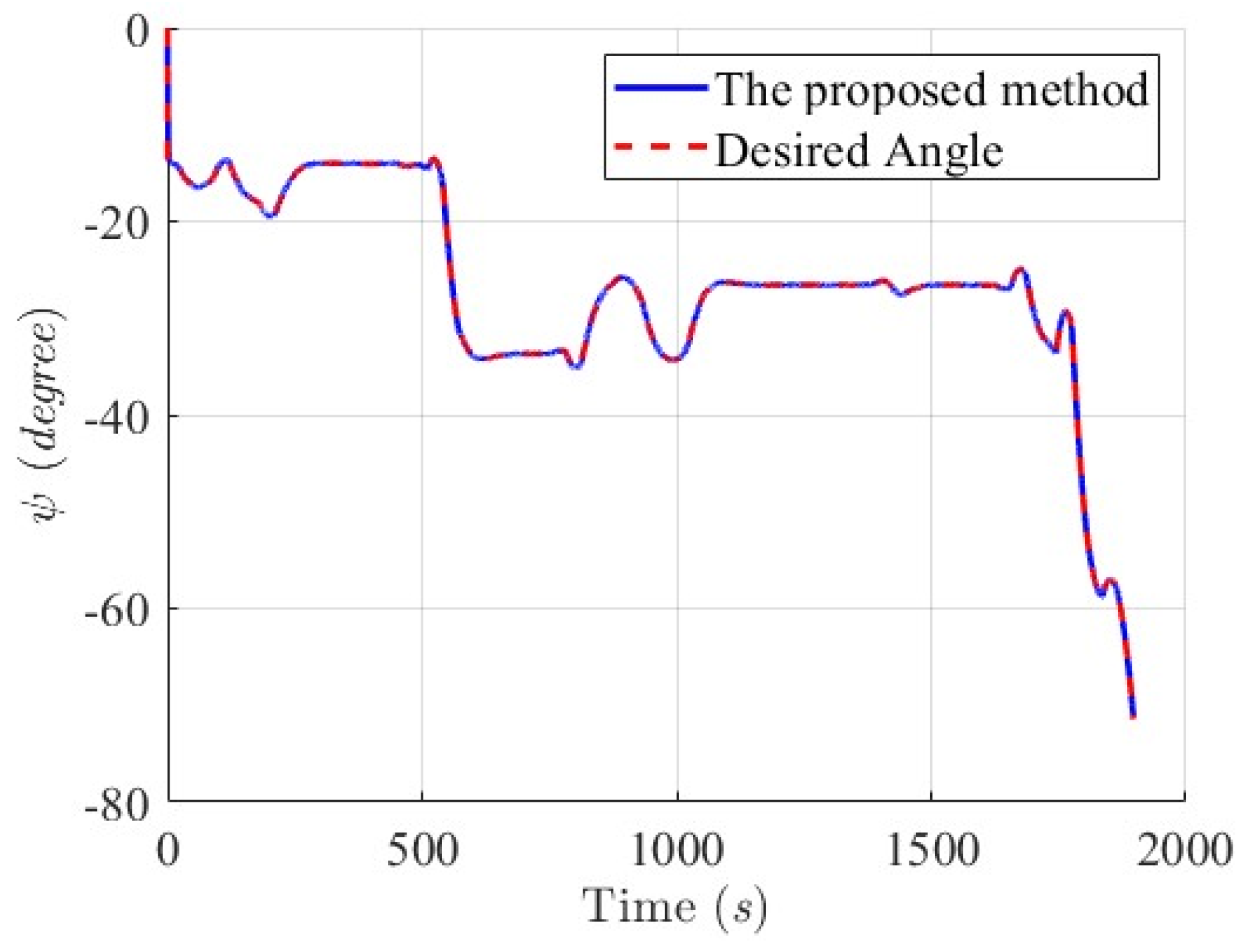
6.2. Simulation Results for Collision-Free and Trajectory-Tracking Verification

Two tough scenarios are executed in this investigation for verifying the collision-free and trajectory-tracking ability of the proposed unified control system. For approaching the real sailing situation, influences of ocean environmental disturbances and modeling uncertainties are fully taken into accounted. The test beds of these two scenarios are Yongxin Harbor and the Agongdian River, in Kaohsiung, Taiwan.

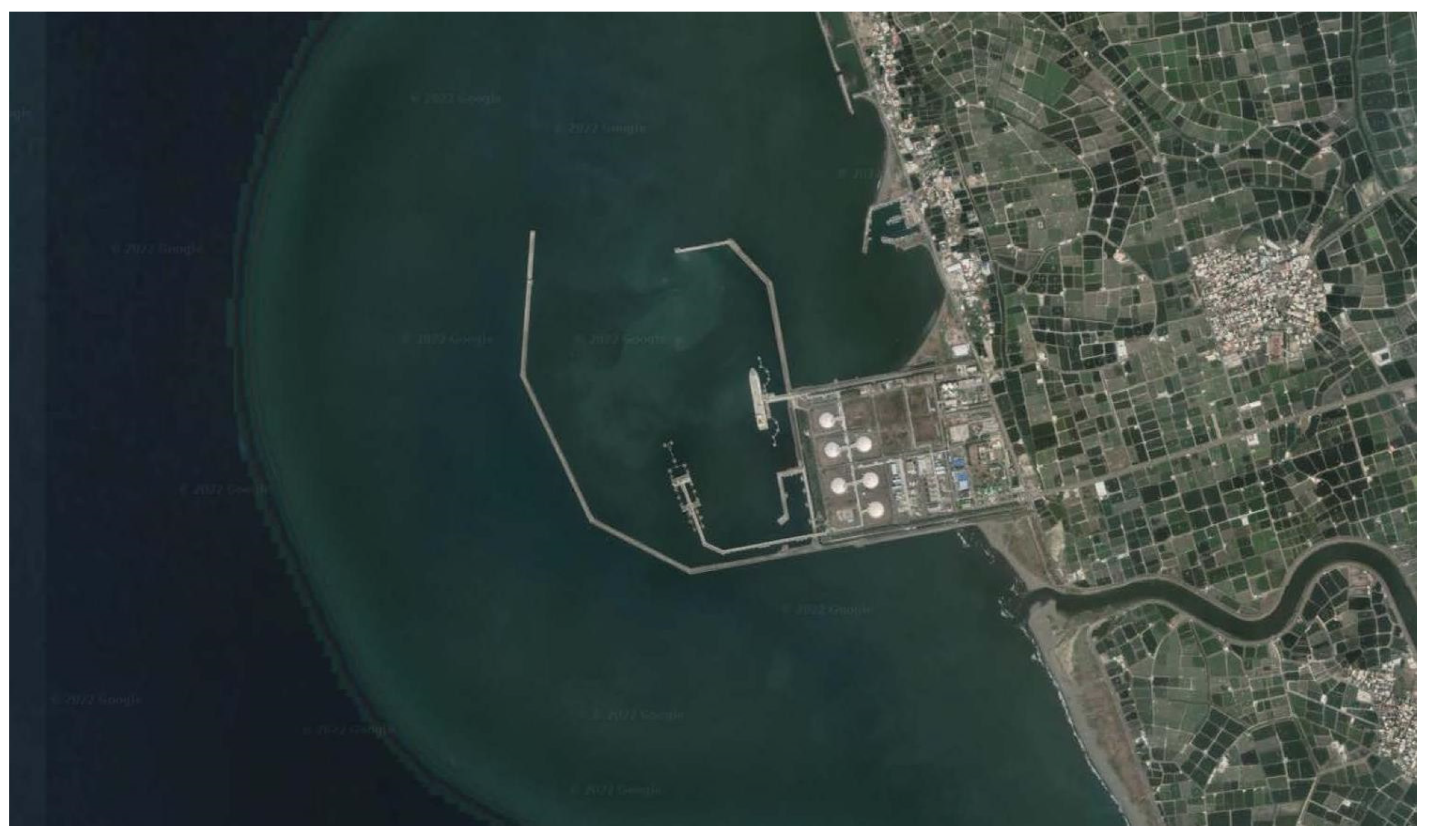
6.2.1. Scenario 1—USV Sails from Open Sea to Yongxin Harbor

The initial simulation arrangement for Scenario 1 is listed in

Table 3. Simulation arrangement of Scenario 1.

Starting Point	(3000 m, 2000 m)
Destination	(2100 m, 3600 m)
Sailing velocity of the controlled USV	1 m/s
Initial Condition	$\eta =\left[\begin{array}{ccc}2999.95& 1999.95& 0^o\end{array}\right]$

. As shown in Figure 14, in this scenario, a set of collision-free waypoints (points 1 to 21) is found based on the double-sided FAA* algorithm. Then, a smooth trajectory (red line) is generated by using the interpolation method of Equation (4) to Equation (7).

In this scenario, the mission task for the proposed unified control system is to control the USV to safely sail from the starting point (point 1) to the destination (point 21). From applying image processing, edge detection, and geofencing construction, two collision-free trajectory segments of the generated total trajectory are delivered between points 5 and 6, where there is a corner of the sea wall and a more complicated area in the inner harbor (point 19 to point 21). This scenario displays a USV that sails from the open sea (left upper corner) to the inner harbor (the right lower corner). This controlled unmanned surface vessel is guided by the proposed nonlinear robust control law to track the generated collision-free trajectory precisely with a designated sailing velocity. From projections of the sailing trajectory on the X and Y axis, the heading angle, etc., as shown in Figure 15, Figure 16, Figure 17, Figure 18, Figure 19 and Figure 20, they indicate the facts that the controlled USV can follow the collision-free trajectory and arrive at the destination (point 21) with pinpoint accuracy. The average trajectory-tracking error is statistically calculated as $\overline{e}={\displaystyle \frac{{\displaystyle \sum _{t=0}^T\sqrt{e_x^2(t)+e_y^2(t)}}}{T_1}}\le 1m$. Here, T₁ is the total sailing time of the controlled USV for achieving Scenario 1. In addition, the heading-angle error $e_{\psi }$ converges to near zero (<1°) under consistent actions of ocean disturbances with a sea state 2 condition.

Histories of the proposed nonlinear robust control law are plotted as follows in Figure 21, Figure 22 and Figure 23. Initially, the control forces and torque are larger for quickly mitigating and guiding the USV to follow the desired trajectory (red line). Since there are two marine structures in the first and second trajectory segments, the negative forces τ_x(t) and τ_y(t) and the torques τ_ψ(t) are delivered to rotate the heading direction of the USV and maintain the sailing paths the within t ∈ [500 s, 1000 s] and t ∈ [1650 s, 1800 s]. Due to the rapid convergent properties of tracking errors $e_x$, $e_y$, and $e_{\psi }$, small control efforts are spent in whole-trajectory-tracking histories once the sailing path of the controlled USV attaches to the desired trajectory.

Since this control allocation method is an analytical solution, it naturally possesses the simplest transformation structure and simultaneously has a low calculation consumption property. By using the control allocation method in Equation (31), ${\mathbf{f}}^{*}={\mathbf{P}}^{-1}{\mathbf{T}}^T{({\mathbf{T}}^T{\mathbf{P}}_a^{-1}\mathbf{T})}^{-1}{\tau }_{\mathrm{E}}$, the corresponding output commands of the installed actuators are revealed in Figure 24, Figure 25, Figure 26 and Figure 27. Based on this advanced control allocation method, the desired robust control commands are well-distributed to the installed rotatable waterjets, and it is found that all of the output commands of the rotatable waterjets that are in Figure 24, Figure 25, Figure 26 and Figure 27 are within the physical limitations, 400 N and ±120°, as revealed in Table 2.

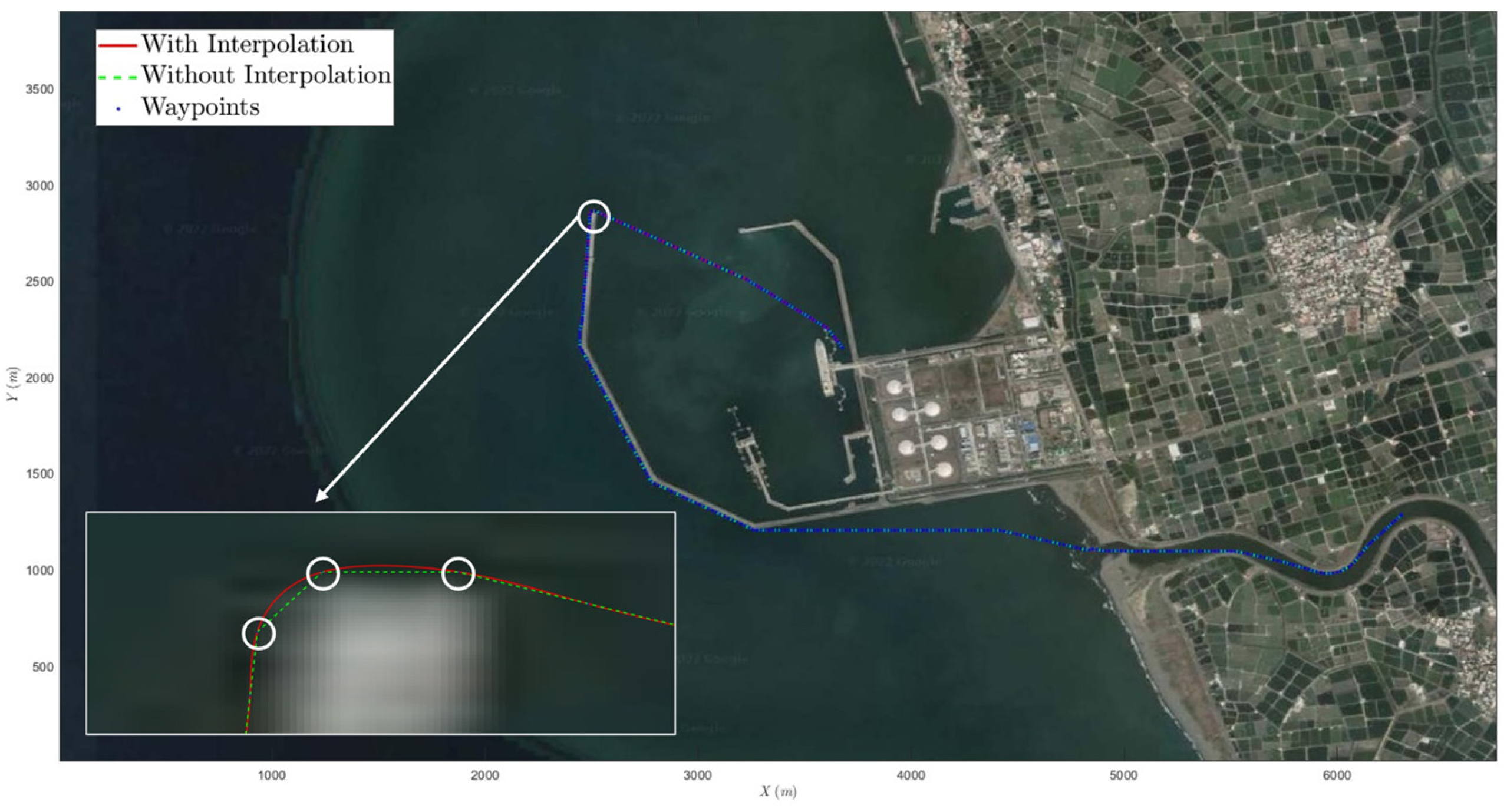
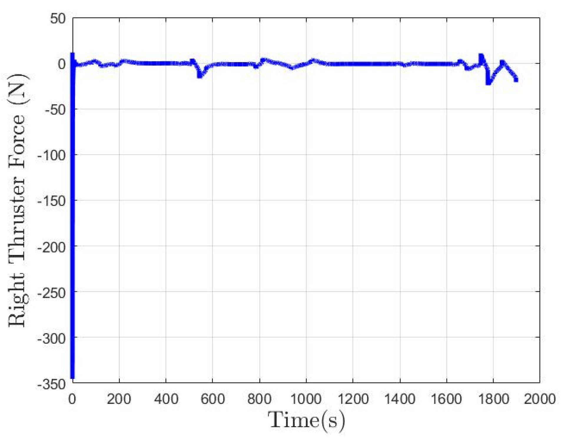
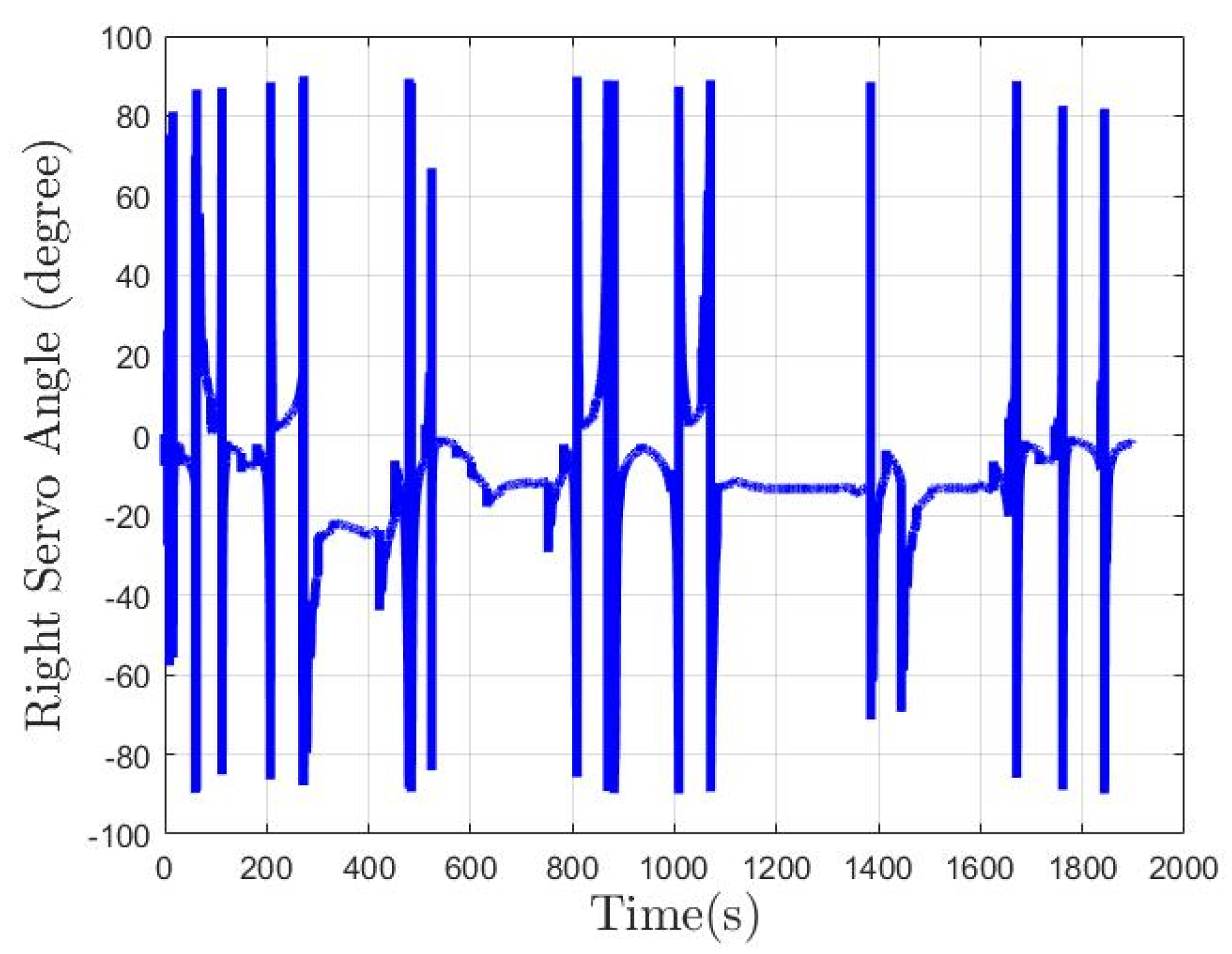
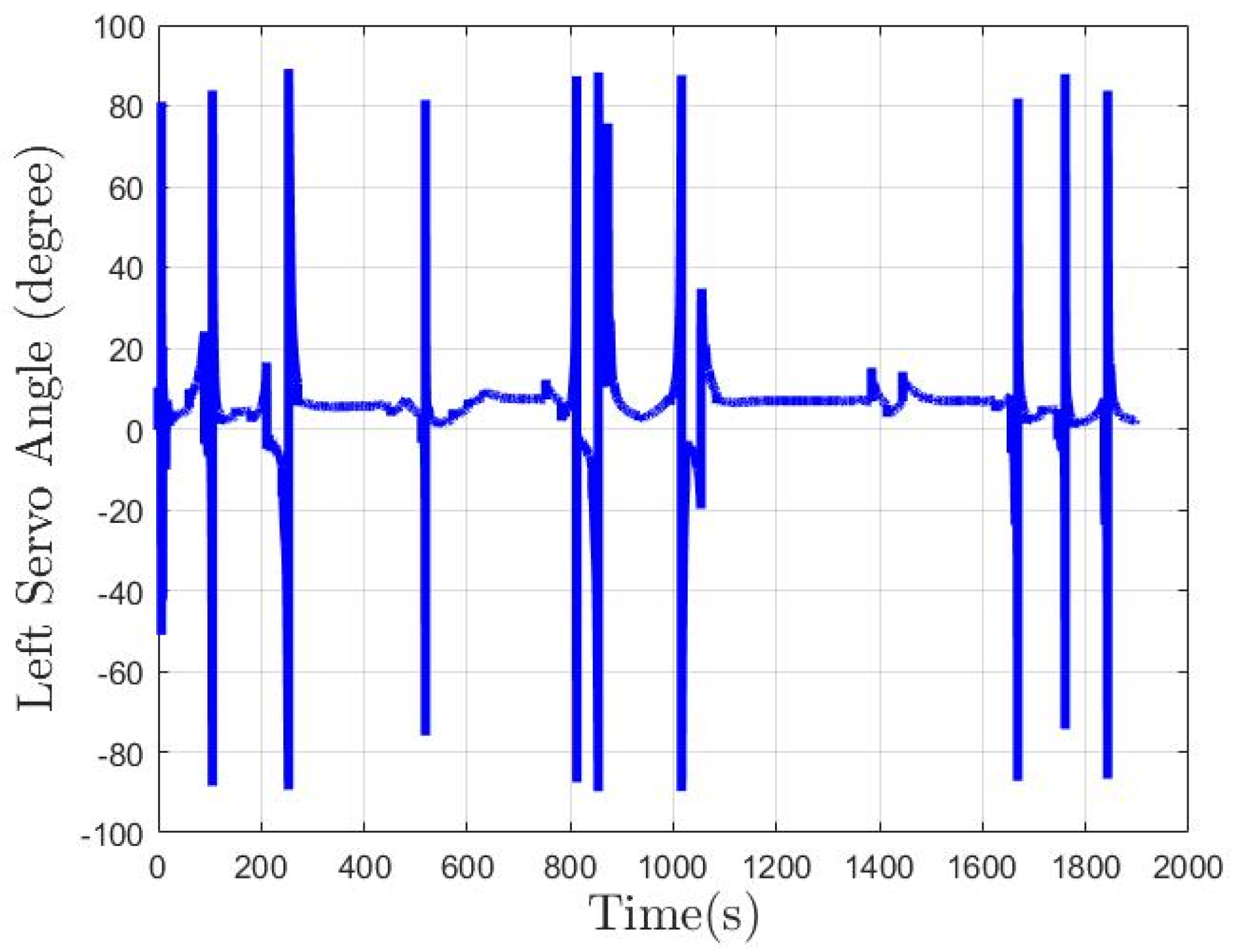
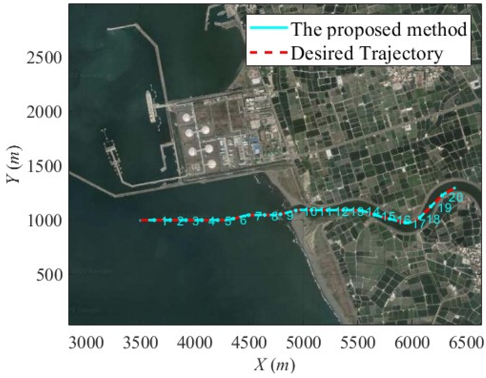
6.2.2. Scenario 2—Agongdian River

In this scenario, the Agongdian River is selected for the verification of this proposed unified control system. The required sailing trajectory of this scenario is complicated because most of the sailing trajectory of this scenario is full of obstacles (point 8~point 20 of Figure 28), such as rocks, banks, and so on. Obviously, Scenario 2 is tougher regarding terrain than Scenario 1, and this issue strongly challenges the searching ability of the proposed trajectory generator and the trajectory-tracking ability of the proposed robust control law.

Arrangements of the initial conditions of the controlled USV, starting point, destination, and desired velocity for Scenario 2 are listed in

Table 4. Details of Scenario 2.

Starting Point	(3500, 1000)
Destination	(6400, 1300)
Desired Velocity	1 m/s
Initial Condition	$\eta =\left[\begin{array}{ccc}3499.95& 999.95& 0\end{array}\right]$

.

Similar to Scenario 1, the proposed unified control system is expected to guide the USV to safely sail from the coast (point 1) to the destination (point 20). From applying image processing, edge detection, and geofencing construction, two collision-free trajectory segments of the generated trajectory have corners of banks between points 12–14 and 16–18.

This scenario displays that a USV sails from the open sea to the inland area. This controlled USV is guided by the proposed nonlinear robust control law to track the generated collision-free trajectory precisely with a designated sailing velocity. The sailing velocity of the controlled USV is maintained at the required 1 m/s, as illustrated in Figure 29. From projections of the sailing trajectory on the X and Y axis, the heading angle, etc., as shown in Figure 30, Figure 31, Figure 32, Figure 33, Figure 34 and Figure 35, all projections attach to the desired ones, and these results reveal the fact that the controlled USV can follow the collision-free trajectory and arrive at the destination (point 20) precisely. The average trajectory-tracking error is $\overline{e}={\displaystyle \frac{{\displaystyle \sum _{t=0}^T\sqrt{e_x^2(t)+e_y^2(t)}}}{T_2}}\le 0.5m$. Here, T₂ is the total sailing time of the controlled USV for achieving Scenario 2. In addition, the heading-angle error $e_{\psi }$ converges to near zero and is bounded within ±0.1°.

The results of the proposed control law are displayed in Figure 36, Figure 37 and Figure 38. Similarly, as for the results in Scenario 1, the control forces and the torque are larger to quickly mitigate and guide the USV in following the desired trajectory (red line). Since there are two turning corners in the collision-free trajectory, the positive and negative forces ${\tau }_x(t)$, ${\tau }_x(t)$ and torques ${\tau }_{\psi }(t)$ are delivered to rotate the heading direction of the USV and maintain the sailing path on the desired trajectory. Transparently, the required control commands of this scenario are lower than those of Scenario 1. The reason is that “In this scenario, most of the desired trajectory are near straight line (point 1 to point 16), and the robust control law outputs lower values once a precise trajectory tracking is executed”.

By using the control allocation method in Equation (31), the corresponding output commands of the installed rotatable waterjets transformed from the desired robust control command are revealed in Figure 39, Figure 40, Figure 41 and Figure 42, and they are within the physical limitations of 400 N and ±120°. As above mentioned, since lower control values are demanded for the proposed robust control law for this scenario, the outputs of the rotatable waterjets, illustrated in Figure 39, Figure 40, Figure 41 and Figure 42, are slower to react to this requirement.

7. Conclusions

A promising unified control system is successfully developed for the collision-free and trajectory-tracking designs of intelligent unmanned surface vessels in this investigation. To the best knowledge of the authors, the published literature devotes all of its energies to constructing a completed control design that combines a collision-free trajectory generator, a nonlinear robust control law, and a control allocation transformation for fulfilling all control, and collision-free requirements of real unmanned devices are rare. This research delivers a unified control system that possesses all of these required properties for the intelligent control design of USVs. The trajectory generator of this proposed unified control system offers a quick and real-time collision-free trajectory generation (run time < 1 s) first. A nonlinear robust control law is then to deliver an effective control command to maintain the controlled unmanned surface vessel to follow the collision-free trajectory in a precise way, even under the effects of modeling uncertainties and ocean disturbances. For approaching the accurate transformation problem between the desired nonlinear robust control command and outputs of actuators, a control allocation method with an analytical solution form is derived. This analytical design has features of a very low complexity structure and a very low calculation power consumption. From two collision-free and trajectory-tracking validations for this proposed unified control system in Yongxin Harbor and on the Agongdian River, respectively, satisfactory control performances “average trajectory-tracking errors ≤1m, can be achieved by this proposed control system even under influences of an ocean disturbance with sea state 2 and 10% of modeling uncertainties”. Finally, the unified control design of a swam of USVs is a potential research area, extending the achievements of this investigation.

References

1. Ships and Shipping of Tomorrow. Available online: https://books.google.com.tw/books/about/Ships_and_Shipping_of_Tomorrow.html?id=WC1UAAAAMAAJ&redir_esc=y (accessed on 1 January 1983).
2. Autonomous Ships Market Expected to Reach US$ 235.73 Bn by 2028. Acute Market Reports. Available online: https://www.acutemarketreports.com/press/global-autonomous-ships-market (accessed on 15 March 2022).
3. Avikus, H.D.H. Successfully Conducts the World’s First Transoceanic Voyage of a Large Merchant Ship Relying on Autonomous Navigation Technologies; HD Hyundai: Seoul, Republic of Korea, 2022. [Google Scholar]
4. Ma, H.; Smart, E.; Ahmed, A.; Brown, D. Radar image-based positioning for USV under GPS denial environment. IEEE Trans. Intell. Transp. Syst. 2018, 19, 72–80. [Google Scholar] [CrossRef]
5. Campbell, S.; Naeem, W.; Irwin, G.W. A review on improving the autonomy of unmanned surface vehicles through intelligent collision avoidance manoeuvres. Annu. Rev. Control 2012, 36, 267–283. [Google Scholar] [CrossRef]
6. Song, R.; Liu, Y.; Bucknall, R. Smoothed A* algorithm for practical unmanned surface vehicle path planning. Appl. Ocean Res. 2019, 83, 9–20. [Google Scholar] [CrossRef]
7. Kim, H.; Kim, S.-H.; Jeon, M.; Kim, J.; Song, S.; Paik, K.-J. A study on path optimization method of an unmanned surface vehicle under environmental loads using genetic algorithm. Ocean Eng. 2017, 142, 616–624. [Google Scholar] [CrossRef]
8. Liu, Y.; Bucknall, R.; Zhang, X. The fast marching method based intelligent navigation of an unmanned surface vehicle. Ocean Eng. 2017, 142, 363–376. [Google Scholar] [CrossRef]
9. Wang, N.; Ahn, C.K. Hyperbolic-tangent LOS guidance-based finite time path following of underactuated marine vehicles. IEEE Trans. Ind. Electron. 2020, 67, 8566–8575. [Google Scholar] [CrossRef]
10. Zheng, Z.; Sun, L.; Xie, L. Error-constrained LOS path following of a surface vessel with actuator saturation and faults. IEEE Trans. Syst. Man Cybern. Syst. 2018, 48, 1794–1805. [Google Scholar] [CrossRef]
11. Li, J.-H.; Lee, P.-M.; Jun, B.-H.; Lim, Y.-K. Point-to-point navigation of underactuated ships. Automatica 2008, 44, 3201–3205. [Google Scholar] [CrossRef]
12. Chen, Y.-Y.; Lee, C.-Y.; Tseng, S.-H.; Hu, W.-M. Nonlinear Optimal Control Law of Autonomous Unmanned Surface Vessels. Appl. Sci. 2020, 10, 1686. [Google Scholar] [CrossRef]
13. Yi, B.; Qiao, L.; Zhang, W. Two-time scale path following of underactuated marine surface vessels: Design and stability analysis using singular perturbation methods. Ocean Eng. 2016, 124, 287–297. [Google Scholar] [CrossRef]
14. Chen, Y.-H.; Tiew, M.Z.E.; Chan, Y.-H.; Lin, G.-W.; Chen, Y.-Y. Trajectory Tracking Design for Unmanned Surface Vessels: Robust Control Approach. J. Mar. Sci. Eng. 2023, 8, 1612. [Google Scholar] [CrossRef]
15. Qin, H.; Chen, H.; Sun, Y.; Chen, L. Distributed finite-time fault tolerant containment control for multiple ocean bottom flying node systems with error constraints. Ocean Eng. 2019, 189, 106341. [Google Scholar] [CrossRef]
16. Abdelhamid, B.; Mohamed, C. Adaptive fuzzy fault-tolerant control using Nussbaum-type function with state-dependent actuator failures. Neu Comp. App 2021, 33, 191–208. [Google Scholar]
17. Yue, H.; Xue, A.; Li, J. Adaptive fuzzy finite-time output feedback fault-tolerant control for MIMO stochastic nonlinear systems with non-affine nonlinear faults. J. Low Freq. Noise Vib. Act. Control 2024, 43, 1312–1338. [Google Scholar] [CrossRef]
18. Sofiane, B.; Mohammed, C.; Salim, Z. The International Conference on Electrical Engineering and Control Applications. In Proceedings of the 4th International Conference on Electrical Engineering and Control Applications, Constantine, Algeria, 17–19 December 2019. [Google Scholar]
19. Yang, J.M.; Chen, Y.-Y.; Tseng, P.S. Real-Time Path Planning for Unmanned Surface Vehicle by using Finite Angle A* Algorithm. J. Taiwan Soc. Nav. Archit. Mar. Eng. 2015, 34, 165–172. [Google Scholar]
Figure 1. The block diagram of the proposed unified control system.
Mathematics 13 00609 g001
Figure 2. Satellite image of the interested region where the controlled USV executes tasks.
Mathematics 13 00609 g002
Figure 3. Binarization result of Figure 2 after applying Otsu’s method.
Mathematics 13 00609 g003
Figure 4. An original binary image (left) and the structuring element (right).
Mathematics 13 00609 g004
Figure 5. Output image and the geofencing (pink color) by using a dilation operation.
Mathematics 13 00609 g005
Figure 6. Dilation result of Figure 2 by using Equation (2).
Mathematics 13 00609 g006
Figure 7. Path-searching result of the FAA* algorithm.
Mathematics 13 00609 g007
Figure 8. Path-searching result of the double-sided FAA* algorithm.
Mathematics 13 00609 g008
Figure 9. The illustration of the searched collision-free waypoints (blue points).
Mathematics 13 00609 g009
Figure 10. The smooth trajectory with several sharp turning angles.
Mathematics 13 00609 g010
Figure 11. Illustration of path planning using collision-free waypoints.
Mathematics 13 00609 g011
Figure 12. The desired smooth trajectory (red color) via using the proposed interpolation algorithm.
Mathematics 13 00609 g012
Figure 13. The appearance of controlled USV.
Mathematics 13 00609 g013
Figure 14. The sailing trajectory of the controlled USV in Scenario 1.
Mathematics 13 00609 g014
Figure 15. Trajectory-tracking history on X axis of Scenario 1.
Mathematics 13 00609 g015
Figure 16. Trajectory-tracking history on Y axis of Scenario 1.
Mathematics 13 00609 g016
Figure 17. Trajectory-tracking history in ψ of Scenario 1.
Mathematics 13 00609 g017
Figure 18. Tracking error on X axis of Scenario 1.
Mathematics 13 00609 g018
Figure 19. Tracking error on Y axis of Scenario 1.
Mathematics 13 00609 g019
Figure 20. Tracking error in ψ axis of Scenario 1.
Mathematics 13 00609 g020
Figure 21. History of the control torque τx of Scenario 1.
Mathematics 13 00609 g021
Figure 22. History of the control torque τy of Scenario 1.
Mathematics 13 00609 g022
Figure 23. History of the control moment τψ of Scenario 1.
Mathematics 13 00609 g023
Figure 24. History of right thruster force for Scenario 1.
Mathematics 13 00609 g024
Figure 25. History of turning angle of right waterjet for Scenario 1.
Mathematics 13 00609 g025
Figure 26. History of left thruster force for Scenario 1.
Mathematics 13 00609 g026
Figure 27. History of turning angle of left waterjet for Scenario 1.
Mathematics 13 00609 g027
Figure 28. Trajectory-tracking history of the controlled USV in Scenario 2.
Mathematics 13 00609 g028
Figure 29. Velocity history of the guided USV in Scenario 2.
Mathematics 13 00609 g029
Figure 30. Trajectory-tracking history on X axis of Scenario 2.
Mathematics 13 00609 g030
Figure 31. Trajectory-tracking history on Y axis of Scenario 2.
Mathematics 13 00609 g031
Figure 32. Trajectory-tracking history in ψ of Scenario 2.
Mathematics 13 00609 g032
Figure 33. Tracking error on X axis of Scenario 2.
Mathematics 13 00609 g033
Figure 34. Tracking error on Y axis of Scenario 2.
Mathematics 13 00609 g034
Figure 35. Tracking error in ψ axis of Scenario 2.
Mathematics 13 00609 g035
Figure 36. History of the control torque τx of Scenario 2.
Mathematics 13 00609 g036
Figure 37. History of the control torque τy of Scenario 2.
Mathematics 13 00609 g037
Figure 38. History of the control moment τψ of Scenario 2.
Mathematics 13 00609 g038
Figure 39. History of right thruster force for Scenario 2.
Mathematics 13 00609 g039
Figure 40. History of turning angle of right waterjet for Scenario 2.
Mathematics 13 00609 g040
Figure 41. History of left thruster force for Scenario 2.
Mathematics 13 00609 g041
Figure 42. History of turning angle of left waterjet for Scenario 2.
Mathematics 13 00609 g042