Energy Efficacy Enhancement in a Reactive Couple-Stress Fluid Induced by Electrokinetics and Pressure Gradient with Variable Fluid Properties

Abstract

This study presents a mathematical analysis of the collective effect of chemical reactions, variable fluid properties, and thermal stability of a hydromagnetic couple-stress fluid flowing through a microchannel driven by electro-osmosis and a pressure gradient. The viscosity of the biofluid is assumed to depend on the temperature, while the electrical conductivity is assumed to be a linear function of the drift velocity. The governing equations are derived non-dimensionalized, and numerical solutions are obtained using the spectral Chebyshev collocation method. The numerical solution is validated using the shooting Runge–Kutta method. The effects of varying the parameters on the thermal stability, temperature, velocity, and entropy profiles are discussed with adequate interpretations using tables and graphs. The results reveal that the chemical reactions and viscosity parameter increase the fluid temperature, while the Hartmann number decreases the temperature and increases the flow velocity and entropy generation. It was also observed that the chemical reactions and viscosity parameter increased the entropy at the channel walls, while the Hartmann number decreased the entropy at the core center of the channel. This study has tremendous empirical significance, including but not limited to biophysical applications of devices, engineering applications such as control systems, and thermo-fluidic transport.

1. Introduction

Due to its applications in many real-life situations, significant progress has been made in studies related to electro-osmotic flow (EOF) with or without pressure gradients. This is due to the fact that electro-osmotic principles are helpful in water treatment, soil percolation, chemical separation analysis, microfluidics apparatus, and scientific, engineering, and industrial applications that deal with electrolysis. Some vital literature on EOF includes that of Elbaighdriri et al. [1], who investigated the EOF of Williamson nanofluids through a convergent tube experiencing double diffusivity with a constant heat source. In [2], Reddy et al. conducted a thermal investigation of the EOF of a nanofluid with wave-like movement through an asymmetrical channel. The study by Tripathi et al. [3] highlighted the collective impacts of peristalsis and electro-osmosis on unsteady electrokinetic fluid flow in a microchannel. Other references related to electro-osmotic flow can be found in [4,5,6,7].

Chemical reactions are significant in energy production, forensic investigations, pool testing equipment, waste management, and metabolism. It also has industrial applications in combustion processes, metal production, and many other applications that have not been mentioned. Based on the foregoing, Raju et al. [8] studied the bearing of binary chemical reactions with activation energy on the convective Maxwell fluid flow through a rotating medium full of porous materials. Tanveer et al. [9] explored the interactions of homogenous and heterogeneous chemical reactions with the electro-osmotic flow of Jeffrey fluid with peristalsis. Prashanth and Rao [10] examined the effect of DuFour and Soret on the equilibrium of the magnetohydrodynamic flow of a chemically reactive nanofluid using the Keller Box technique. Other notable literature has been written on chemical reactions [11,12,13,14].

Recent findings [15,16,17,18,19,20,21] have shown that variable fluid properties are more appropriate for describing many complex fluids. In actual sense, these properties: viscosity, density, electrical conductivity, porous permeability, and many others vary with time, space, temperature, and velocity. The temperature-dependent viscosity and velocity-dependent electrical conductivity of the fluid are of interest here. In [15], Prasad et al. reported the outcome of varying thermal and viscosity conductivities on steady hydromagnetic flow over a stretched surface. Adeyemo et al. [16] addressed the fully developed nonlinear flow of an incompressible fluid bounded by a vertical channel saturated with permeable materials without heat transfer at the walls; the fluid’s viscosity was assumed to be linearly dependent on temperature. Wu and Pruess [17] applied the integral method to obtain analytic solutions to a transient movement of a compressible fluid across a porous medium, with the permeability taken as a function of pressure.

The thermal stability of fluids is the ability of a reactive fluid to resist spontaneous ignition due to heat generation and dissipation. The auto-ignition temperature is the lowest temperature at which fluids will self-combust. The study of the thermal stability of materials has become increasingly important due to its various applications in energy storage and conversion, safe working environments, medical electronic devices, pharmaceuticals, and chemical processes, for example, in the production of polymers. Given these different applications, numerous authors [22,23,24,25,26,27,28] have investigated and discussed the thermal stability of various reactive fluids. Adeosun and Ukaegbu [22] performed a thermal criticality analysis of squeezed fluid flowing along parallel plates with variable electrical conductivity. The study by Salawu et al. [23] reported the thermal stability of Williamson reactive fluid with combined isotropic nanoparticles under thin radiation. Adesanya et al. [24] examined the thermal stability of a reactive fluid flowing through a porous medium and demonstrated the role of heat dissipation in stability control.

The originality of our work lies in the inclusion of reaction kinetics (in the form of Arrhenius, Sensitized, and Bimolecular), temperature-dependent viscosity, and velocity-dependent electrical conductivity, which were not considered in the previous study [7]. Our study provides a broad-based approach to biophysical systems and thermal engineering. Additionally, the inclusion of thermal stability analysis in the combustible exothermic system introduces a novel perspective not extensively addressed in earlier works. From an application viewpoint, physical fluid properties are not constant in many real-life situations. For instance, electrical conductivity varies with ion size, temperature [29], and, most importantly, drift velocity, even in biofluids like blood [30]. This is especially true when the working fluid has haphazardly oriented and rigid particles and substructures, which are features of a couple of stress fluids. For other related works, refer [31,32,33]. These variations are expected to better approximate the electro-osmotic flow, especially in many thermal engineering applications involving flow rate and varying temperature due to chemical interactions. In addition, after an exhaustive survey of the literature on electro-osmotic flows of a couple of stress fields, there is no report on chemical reactions and variable electrical conductivity, which varies with drift velocity; this highlights the significance of the research. The study outcomes for the temperature, velocity, and entropy profiles are displayed pictorially, and the physical interpretations are reported comprehensively. The results for validating the solution, convergence, and thermal stability are tabulated for varying parameters. Furthermore, the results reveal that the temperature and flow velocity magnitude increase when the variable viscosity parameter increases.

2. Model Derivation

We examine the steady flow of a non-compressible EMHD couple-stress fluid along an unending horizontal channel at $z=-Handz=H$, which can be seen in Figure 1.

2.1. Derivation of Potential Distribution

To drive the fluid flow in the axial direction, we need to determine the potential distribution within the system. The electrochemical potential, which is the combination of the electrical and chemical potential, is given as,

$$\mu ={\mu }_0+k_{B}TIn\left(n\right)+Ze\psi \prime$$

(1)

where, ${\mu }_0$ is the reference potential, $n$ is the number density (concentration), $T$ is the room temperature, $Z$ is the valency, $e$ is the protonic charge, $\psi \prime$ is the electric potential, $k_B$ is the Boltzmann constant.

Imposing the electrochemical equilibrium condition on (1), we obtain the following Boltzmann distribution equation,

$$n=n_0{e}^{-{\displaystyle \frac{Ze{\psi }^{\prime }}{k_{B}T}}}$$

(2)

where the positive and negative ions, positive and negative valency are respectively given as,

$$n^{+}=n_0{e}^{-{\displaystyle \frac{Z^{+}e{\psi }^{\prime }}{k_{B}T}}},n^{-}=n_0{e}^{-{\displaystyle \frac{Z^{-}e{\psi }^{\prime }}{k_{B}T}}},Z^{+}=Z,Z^{-}=-Z$$

(3)

Applying the Gauss’ Law to relate the charge density with the electric field, we obtain

$${\epsilon }_0\underset{S}{{\displaystyle \oint }}\overrightarrow{E}•d\overrightarrow{S}=\underset{V}{{\displaystyle \int }}{({\rho }_e)}_{total}dV=\underset{V}{{\displaystyle \int }}\left[-\nabla •\left({\epsilon }_0\chi \overrightarrow{E}\right)+{\rho }_e\right]dV$$

(4)

with

$$\begin{array}{ll}{({\rho }_e)}_{total}& ={({\rho }_e)}_{free}+{({\rho }_e)}_{bound}\\ & ={({\rho }_e)}_{free}-\nabla •\overrightarrow{P}\\ & ={({\rho }_e)}_{free}-\nabla •{\epsilon }_0\chi \overrightarrow{E}\end{array}$$

(5)

By applying the Gauss’ divergence theorem, we obtain the Poisson-type equation,

$$\nabla •\left[\epsilon \overrightarrow{E}\right]={\rho }_e$$

(6)

where $\overrightarrow{E}:$ Electric field, ${\epsilon }_0:$ free space permittivity, $d\overrightarrow{S}:$ surface element, ${({\rho }_e)}_{total}:$ total volumetric charge density, $dV:$ volume element, $\overrightarrow{P}:$ polarization vector, $\chi :$ susceptibility of the medium. $\epsilon ={\epsilon }_0\left(1+\chi \right):$ total permittivity.

Using $\overrightarrow{E}=-\nabla {\psi }^{\prime }$, we obtain the Laplacian equation,

$${\nabla }^2{\psi }^{\prime }={\displaystyle \frac{-{\rho }_e}{\epsilon }}$$

(7)

The free charge density is the sum total of negative and positive ions, ${\rho }_e=\sum Ze{n}_i,(i=1,2,)$ therefore,

$$\epsilon {\displaystyle \frac{d^2{\psi }^{\prime }}{d{z}^{\prime 2}}}=\left(n^{-}-n^{+}\right)Ze$$

(8)

$$\epsilon {\displaystyle \frac{d^2{\psi }^{\prime }}{d{z}^{\prime 2}}}=n_{0}Ze\left[e^{{\displaystyle \frac{Ze{\psi }^{\prime }}{k_{B}T}}}-e^{-{\displaystyle \frac{Ze{\psi }^{\prime }}{k_{B}T}}}\right]=2n_{0}Zesinh\left[{\displaystyle \frac{Ze{\psi }^{\prime }}{k_{B}T}}\right]$$

(9)

The nonlinear equation above is called the Poisson-Boltzmann equation. By using the Debye–Hückel linearization for ${\displaystyle \frac{Ze{\psi }^{\prime }}{k_{B}T}}<<1$, that is, $sinh\left[{\displaystyle \frac{Ze{\psi }^{\prime }}{T_a{k}_B}}\right]\approx {\displaystyle \frac{Ze{\psi }^{\prime }}{T_a{k}_B}}$, we obtain

$${\displaystyle \frac{d^2{\psi }^{\prime }}{d{z}^{\prime 2}}}={\displaystyle \frac{2n_0{Z}^2{e}^2}{\epsilon k_B{T}_a}}{\psi }^{\prime }=k^2{\psi }^{\prime }$$

(10)

together with the symmetric and slip conditions to solve the equation.

$${\left.{\displaystyle \frac{d{\psi }^{\prime }}{d{z}^{\prime }}}\right|}_{z^{\prime }=0}=0and{\left.{\psi }^{\prime }\right|}_{z^{\prime }=H}=\zeta \mathrm{and}$$

(11)

where $k:$ inverse Debye Length, $\zeta =Max\left[{\psi }^{\prime }\right]:$ zeta potential.

Finally, the solution of (10) subject to (11) satisfies,

$${\rho }_e\left(z^{\prime }\right)={\displaystyle \frac{-\epsilon k^2\zeta \cosh \left(k{z}^{\prime }\right)}{\cos \mathrm{h}\left(kH\right)}}$$

(12)

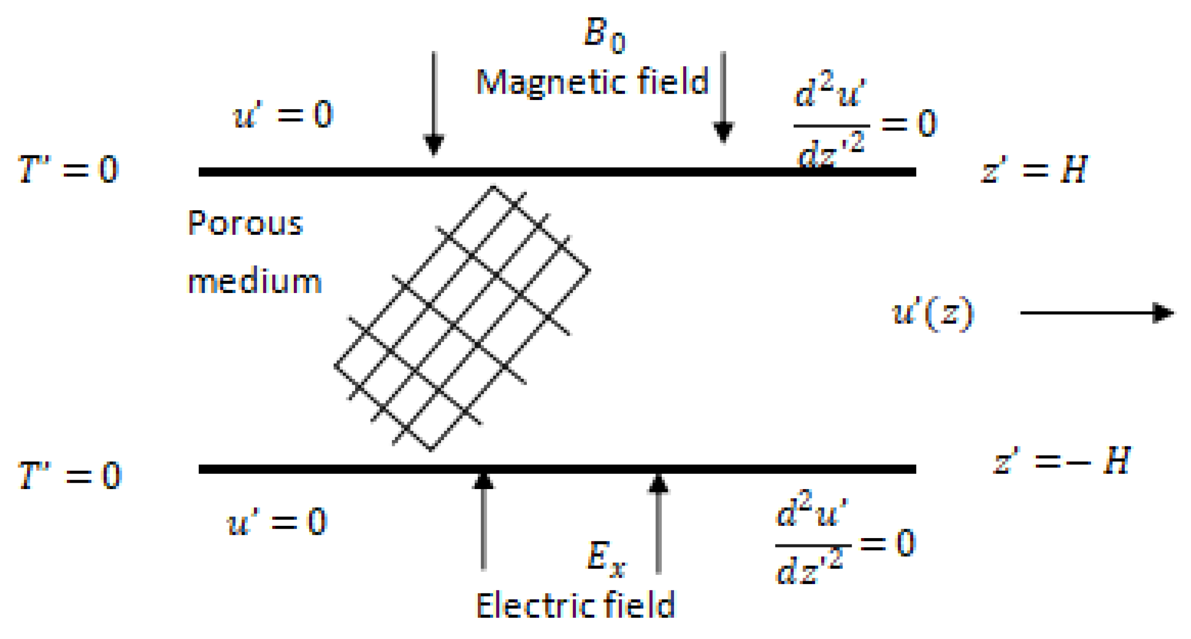
2.2. Conservation of Mass and Momentum

In this work, the steady flow of reactive couple-stress fluid through a porous medium is considered. The flow is driven by electro-osmotic force together with a pressure gradient. We also examine the effect of variable porous permeability, viscosity, and electrical conductivity. The viscosity of the flow and porous permeability are assumed to be dependent on the width of the microchannel. The electrical conductivity also depends on the flow velocity (Sivaraj and Kumar [21]). The biofluid considered in this study is blood, whose viscosity depends on temperature.

For this model, we have the following assumptions

• The flow is steady, hydrodynamically and thermally fully developed,
• The flow is unidirectional, hence $\overrightarrow{u}=\left(u^{\prime }\left(z\prime \right),0,0\right)and\overline{T}=\left(T\prime \left(z\prime \right),0,0\right)$
• The electric field $\overrightarrow{E}=\left(E_x,E_y,0\right)$ is applied along the $x\prime$ and $y\prime$ directions.
• The magnetic field $\overrightarrow{B}=\left(0,0,B_0\right)$ is imposed along the $z\prime$ direction.
• $\overrightarrow{J}=\sigma \left(\overrightarrow{E}+\overrightarrow{u}\times \overrightarrow{B}\right)$

The modified momentum equation, therefore, becomes

$$-{\displaystyle \frac{dP}{dx\prime }}+{\displaystyle \frac{d}{dz\prime }}\left(\mu (T){\displaystyle \frac{du\prime }{dz\prime }}\right)-\eta {\displaystyle \frac{d^{4}u\prime }{dz{\prime }^4}}-{\displaystyle \frac{\epsilon k^2{E}_x\zeta \cosh \left(k{z}^{\prime }\right)}{\cosh \left(kH\right)}}+{\sigma }_e{E}_y{B}_0-{\sigma }_e{B_0}^{2}u\prime =0$$

(13)

with the no-slip and non-moving wall conditions given as,

$${\left.u\prime \left(z\prime \right)\right|}_{z^{\prime }=\pm H}=0{\left.and{\displaystyle \frac{d^2{u}^{\prime }}{d{z}^{\prime 2}}}\right|}_{z^{\prime }=\pm H}=0\mathrm{and}$$

(14)

where

$${\sigma }_e={\sigma }_{0}u,\mu \left(T^{\prime }\right)={\mu }_0{e}^{{\alpha }^{\prime }\left(T_0-T^{\prime }\right)}$$

(15)

To make the equation dimensionless, we use the following parameters,

$$\left.\begin{array}{l}{U}_{HS}={\displaystyle \frac{\epsilon E_x\zeta }{{\mathsf{\mu }}_0}},z={\displaystyle \frac{z^{\prime }}{H}},u={\displaystyle \frac{u^{\prime }}{U_{HS}}},\kappa =kH,\mathsf{\Omega }=-{\displaystyle \frac{H^2}{{\mathsf{\mu }}_0{U}_{HS}}}{\displaystyle \frac{dP}{dx\prime }},\\ Ha=B_{0}H\sqrt{{\displaystyle \frac{{\sigma }_0}{{\mathsf{\mu }}_0}}},S={\displaystyle \frac{E_{y}H}{U_{HS}}}\sqrt{{\displaystyle \frac{{\sigma }_0}{{\mathsf{\mu }}_0}}},\gamma =\sqrt{{\displaystyle \frac{{\mathsf{\mu }}_0{H}^2}{\eta }}}\end{array}\right\}$$

(16)

Applying these parameters above, we obtain the dimensionless equation,

$$\left.\begin{array}{l}\mathsf{\Omega }+{\displaystyle \frac{d}{dz}}\left[e^{-{\alpha }_1\theta }{\displaystyle \frac{du}{dz}}\right]-{\displaystyle \frac{1}{{\gamma }^2}}{\displaystyle \frac{d^{4}u}{d{z}^4}}-{\kappa }^2{\displaystyle \frac{\cosh \left(\kappa z\right)}{\cosh \left(\kappa \right)}}+SHau-H{a}^2{u}^2=0\\ u\left(\pm 1\right)=0{\left.,{\displaystyle \frac{d^{2}u}{d{z}^2}}\right|}_{z=\pm 1}=0\end{array}\right\}$$

(17)

Evidently, the exact solution to the above boundary-value problem is only possible when both ${\alpha }_1$ and $Ha$ approach zero.

2.3. Conservation of Energy

The total energy in the control volume is the sum of the kinetic energy and nonlinear internal heat energy. With the addition of chemical reaction term to the model, we arrive at the energy equation,

$$0=k_f\left({\displaystyle \frac{d^2{T}^{\prime }}{d{z}^{\prime 2}}}\right)+Q{C}_0\mathrm{A}{\left({\displaystyle \frac{hT\prime }{\upsilon l}}\right)}^m{e}^{{\displaystyle \frac{-E}{RT\prime }}}+\mathsf{\mu }\left(T^{\prime }\right){\left({\displaystyle \frac{du\prime }{dz\prime }}\right)}^2+\mathsf{\eta }{\left({\displaystyle \frac{d^{2}u\prime }{dz{\prime }^2}}\right)}^2+{\sigma }_e\left({E_x}^2+{E_y}^2-2E_y{B}_{0}u\prime +{B_0}^{2}u{\prime }^2\right)$$

(18)

and the boundary conditions, ${\left.T\prime \left(z\prime \right)\right|}_{z^{\prime }=\pm H}=T_0$.

We make use of the following dimensionless parameters to non-dimensionalize the energy equation.

$$\left.\begin{array}{l}\theta ={\displaystyle \frac{E(T^{\prime }-T_0)}{R{T}_0^2}},{\alpha }_1={\displaystyle \frac{{\alpha }^{\prime }R{T}_0^2}{E}},s_x={\displaystyle \frac{{\sigma }_0{E}_x^2{H}^2}{{\mu }_0{U}_{HS}^2}},s_y={\displaystyle \frac{{\sigma }_0{E}_y^2{H}^2}{{\mu }_0{U}_{HS}^2}},\\ \beta ={\displaystyle \frac{R{T}_0}{E}},\lambda ={\displaystyle \frac{Q{C}_{0}AE{H}^2}{k_{f}R{T}_0^2}}{\left({\displaystyle \frac{h{T}_0}{\upsilon l}}\right)}^m{e}^{{\displaystyle \frac{-E}{R{T}_0}}},\delta ={\displaystyle \frac{{\mu }_0{U}_{HS}^2}{Q{C}_{0}A{H}^2}}{\left({\displaystyle \frac{\upsilon l}{h{T}_0}}\right)}^m{e}^{{\displaystyle \frac{E}{R{T}_0}}}\end{array}\right\}$$

(19)

The dimensionless form of the modified combustion equation is given as,

$$\left.\begin{array}{l}{\displaystyle \frac{d^2\theta }{d{z}^2}}+\lambda \left[{\left(1+\beta \theta \right)}^m{e}^{{\displaystyle \frac{\theta }{1+\beta \theta }}}+\delta \left(e^{-{\alpha }_1\theta }{\left({\displaystyle \frac{du}{dz}}\right)}^2+{\displaystyle \frac{1}{{\gamma }^2}}{\left({\displaystyle \frac{d^{2}u}{d{z}^2}}\right)}^2+\left(s_x+s_y\right)u-2SHa{u}^2+H{a}^2{u}^3\right)\right]=0\\ \theta \left(\pm 1\right)=0.\end{array}\right\}$$

(20)

The shear stress and wall heat flux are respectively defined as,

$${\tau }_w=\mu \left(T^{\prime }\right){\displaystyle \frac{du\prime }{dz\prime }}-\eta {\left.{\displaystyle \frac{d^{3}u\prime }{dz{\prime }^3}}\right|}_{z=-1}{q}_w=-k_f{\left.{\displaystyle \frac{dT\prime }{dz\prime }}\right|}_{z=-1}$$

(21)

2.4. Entropy Generation Analysis

The local volumetric rate of entropy generation is expressed as

$$E_G={\displaystyle \frac{k_f}{{T_0}^2}}{\left({\displaystyle \frac{dT\prime }{dz\prime }}\right)}^2+{\displaystyle \frac{1}{T_0}}\left[\mu (T^{\prime }){\left({\displaystyle \frac{du\prime }{dz\prime }}\right)}^2+\mathsf{\eta }{\left({\displaystyle \frac{d^{2}u\prime }{dz{\prime }^2}}\right)}^2+{\sigma }_e\left({E_x}^2+{E_y}^2-2E_y{B}_0{u}^{\prime }+{B_0}^2{u}^{\prime 2}\right)\right]$$

(22)

The non-dimensional entropy generation is given as,

$$N_S=\underset{N_{HT}}{\underbrace{{\left({\displaystyle \frac{d\theta }{dz}}\right)}^2}}+\underset{N_{VD}}{\underbrace{{\displaystyle \frac{\lambda \delta }{\beta }}\left[e^{-{\alpha }_1\theta }{\left({\displaystyle \frac{du}{dz}}\right)}^2+{\displaystyle \frac{1}{{\gamma }^2}}{\left({\displaystyle \frac{d^{2}u}{d{z}^2}}\right)}^2+\left(s_x+s_y\right)u-2SHa{u}^2+H{a}^2{u}^3\right]}}$$

(23)

We introduce the Bejan number, $Be$, to evaluate the effect of each parameter on the entropy generation profile. It is given as,

$$Be={\displaystyle \frac{N_{HT}}{N_S}}$$

(24)

A total of 14 non-dimensional parameters are used in this study, namely, Hartmann number, activation energy parameter, electric field parameter, $(Ha,\beta ,S)$, coefficient of viscosity, couple-stress parameter, electrokinetic width, $({\alpha }_1,\gamma ,K)$, velocity, temperature and pressure gradient, $(u,\theta ,\mathsf{\Omega })$, Frank-Kameneskii parameter, entropy generation, $(\lambda ,N_S)$, viscous dissipation parameter, Joule heat parameters $(\delta ,s_x,s_y)$ respectively.

3. Method of Solution

The solutions to the nonlinear Equations (17) and (20) are obtained via the spectral collocation method. The spectral Chebyshev collocation method is chosen for its high accuracy and efficiency in solving complex boundary-value problems. This method is particularly effective for problems involving sharp gradients, as it minimizes computational error and achieves rapid convergence. Validation using the shooting Runge–Kutta method confirms the robustness of this approach, as shown in

Table 1. (a) Validation for velocity when $\beta =0.1;m=0.5;S=1;R=1;H=0.2;\Lambda =1;\gamma =1;\lambda =0.1;{\alpha }_1=0.01;s_1=0.02;\delta =3;\kappa =1;$ (b) Validation for temperature when $\beta =0.1;m=0.5;S=1;R=1;H=0.2;\Lambda =1;\gamma =1;\lambda =0.1;{\alpha }_1=0.01;s_1=0.02;\delta =3;\kappa =1$.

		(a)
$z$	$u{\left(z\right)}_{SCCM}$	$u{\left(z\right)}_{RK4}$	$\left|u{\left(z\right)}_{SCCM}-u{\left(z\right)}_{RK4}\right|$
$-1$	$1.278457061874004\times {10}^{-17}$	$0.$	$1.374898306521335\times {10}^{-18}$
$-0.75$	$0.0629067528195136$	$0.06290675639956234$	$1.212604495981484\times {10}^{-9}$
$-0.5$	$0.11300454429091983$	$0.11300454648432434$	$1.801353691210927\times {10}^{-9}$
$-0.25$	$0.14291696897585213$	$0.14291696903977355$	$3.64452736045795\times {10}^{-9}$
$0.0$	$0.14993371862224614$	$0.1499337180703369$	$4.460718419641019\times {10}^{-9}$
$0.25$	$0.13487591971840526$	$0.13487591943819496$	$7.535644719336432\times {10}^{-9}$
$0.5$	$0.10117000646607631$	$0.10117000659895337$	$1.110966178774486\times {10}^{-8}$
$0.75$	$0.05407250188183676$	$0.05407250280453991$	$1.011271340278785\times {10}^{-8}$
$1.0$	$8.037935726473451\times {10}^{-19}$	$1.538216525204596\times {10}^{-9}$	$6.650356695509854\times {10}^{-10}$
		(b)
$z$	$\theta {\left(z\right)}_{SCCM}$	$\theta {\left(z\right)}_{RK4}$	$\left|\theta {\left(z\right)}_{SCCM}-\theta {\left(z\right)}_{RK4}\right|$
$-1$	$8.347506626484343\times {10}^{-18}$	$0.$	$6.650507319668297\times {10}^{-18}$
$-0.75$	$0.03058197395534581$	$0.030581968580185397$	$3.975948570378307\times {10}^{-9}$
$-0.5$	$0.05284437821144731$	$0.05284437008583946$	$4.714958777574107\times {10}^{-9}$
$-0.25$	$0.06602942949986432$	$0.066029424266624$	$2.094374902672502\times {10}^{-9}$
$0.0$	$0.06989972223532497$	$0.06989971497358342$	$7.650101385703323\times {10}^{-10}$
$0.25$	$0.06470574644977296$	$0.0647057366257331$	$2.431655009293987\times {10}^{-9}$
$0.5$	$0.05096126175034675$	$0.050961251931184746$	$4.9188363451802\times {10}^{-9}$
$0.75$	$0.029232629710794485$	$0.029232620363145338$	$6.575776253375798\times {10}^{-9}$
$1.0$	$-3.288932058159692\times {10}^{-18}$	$-6.386044694272373\times {10}^{-9}$	$7.039165616692663\times {10}^{-9}$

and

Table 2. Exact Solution versus Numerical Solution $\beta =0.1;m=0.5;S=1;R=1;H=0;\Lambda =1;\gamma =1;\lambda =0.1;{\alpha }_1=0;s_1=0.02;\delta =3;\kappa =1$.

$\mathit{z}$	$\mathit{u}{(\mathit{z})}_{\mathit{E}\mathit{x}\mathit{a}\mathit{c}\mathit{t}}$	$\mathit{u}{(\mathit{z})}_{\mathit{S}\mathit{C}\mathit{C}\mathit{M}}$	$\mathit{u}{(\mathit{z})}_{\mathit{E}\mathit{x}\mathit{a}\mathit{c}\mathit{t}}-\mathit{u}{(\mathit{z})}_{\mathit{S}\mathit{C}\mathit{C}\mathit{M}}$
$-1$	$0.$	$-3.325780086847037\times {10}^{-18}$	$3.325780086847037\times {10}^{-18}$
$-0.75$	$0.06218675003473847$	$0.062186750034738315$	$1.52655665885959\times {10}^{-16}$
$-0.5$	$0.11167226783139574$	$0.11167226783139575$	$1.387778780781445\times {10}^{-17}$
$-0.25$	$0.14117656707847842$	$0.14117656707847837$	$5.551115123125783\times {10}^{-17}$
$0.0$	$0.14805427366388543$	$0.14805427366388538$	$5.551115123125783\times {10}^{-17}$
$0.25$	$0.13314676750126822$	$0.13314676750126817$	$5.551115123125783\times {10}^{-17}$
$0.5$	$0.09985338386132184$	$0.09985338386132184$	$0.$
$0.75$	$0.053363321317313625$	$0.053363321317313556$	$6.938893903907228\times {10}^{-17}$
$1.0$	$0.$	$-1.578342750457657\times {10}^{-17}$	$1.578342750457657\times {10}^{-17}$

.

Assume admissible trial polynomials of the form ${\mathsf{\Psi }}_k(z)$ with

$$\left.\begin{array}{l}u\left(z\right)\approx u^N\left(z\right)={\displaystyle \sum _{k=0}^N{b}_k{\mathsf{\Psi }}_k\left(z\right)},\\ \theta \left(z\right)\approx {\theta }^N\left(z\right)={\displaystyle \sum _{k=0}^N{c}_k{\mathsf{\Psi }}_k\left(z\right)}\end{array}\right\}$$

(25)

In (25), ${\mathsf{\Psi }}_k(z)$ is the spectral Chebyshev polynomial with the unknown constants $\left(b_k,c_k\right)$ satisfying boundary conditions. Substituting (25) into the boundary-value problem (17) and (20) gives the subsequent residues that must be solved at specific grid points,

$$\left.\begin{array}{l}{R}_1=\mathsf{\Omega }+{\left(e^{-{\alpha }_1{\theta }^N}{u}_z^N\right)}^{\prime }-{\displaystyle \frac{1}{{\gamma }^2}}{u}_{zzzz}^N-{\displaystyle \frac{{\kappa }^2\cosh (\kappa z)}{\cosh (\kappa )}}+SHa{u}^N-H{a}^2{u}^{2N},\\ R_2={\theta }_{zz}^N+\lambda \left[{\left(1+\beta {\theta }^N\right)}^m{e}^{{\displaystyle \frac{{\theta }^N}{1+\beta {\theta }^N}}}+\delta \left(e^{-{\alpha }_1{\theta }^N}{\left(u_z^N\right)}^2+{\displaystyle \frac{1}{{\gamma }^2}}{\left(u_{zz}^N\right)}^2+\left(s_x+s_y\right)u^N-2SHa{u}^{2N}+H{a}^2{u}^{3N}\right)\right]\end{array}\right\}$$

(26)

with boundary conditions

$$u^N\left(-1\right)=0=u^N\left(1\right),{\left.u_{zz}^N\right|}_{z=-1}=0={\left.u_{zz}^N\right|}_{z=1},{\theta }^N\left(-1\right)=0={\theta }^N\left(1\right)$$

(27)

where $z_k$ are points within $[-1,1]=[z_{0,}{z}_N]$. Then the Gauss-Lobato collocation points are given as

$$z_k=\left(-\cos \left({\displaystyle \frac{i\pi }{N}}\right)\right),i=0,1,2,,N$$

(28)

The residues are solved at the points

$$R_1\left(z_k\right)=0,\mathrm{and}{R}_2\left(z_k\right)=0,k=0,1,2,,N$$

(29)

and the lth-derivatives for dependent variables are obtained as

$${\displaystyle \frac{d^{l}u}{d{z}^l}}={\displaystyle \sum _{i=0}^N{b}_i\frac{d^l{u}_i}{d{z}^l}}\mathrm{and}{\displaystyle \frac{d^l\theta }{d{z}^l}}={\displaystyle \sum _{i=0}^N{c}_i\frac{d^l{\theta }_i}{d{z}^l}}$$

(30)

with the differentiation matrix at each collocation point given as

$$\begin{array}{l}{\displaystyle \frac{d\overline{u}}{dz}}=D^{(1)}\overline{u}=D\overline{u}{\displaystyle \frac{d\overline{\theta }}{dz}}=D^{(1)}\overline{\theta }=D\overline{\theta }\\ {\displaystyle \frac{d^2\overline{u}}{d{z}^2}}=D^{(2)}\overline{u}=D^2\overline{u}and{\displaystyle \frac{d^2\overline{\theta }}{d{z}^2}}=D^{(2)}\overline{\theta }=D^2\overline{\theta }\\ \dots \dots \dots \dots \dots \dots \dots \dots \\ {\displaystyle \frac{d^l\overline{u}}{d{z}^l}}=D^{(l)}\overline{u}=D^l\overline{u}{\displaystyle \frac{d^l\overline{\theta }}{d{z}^l}}=D^{(l)}\overline{\theta }=D^l\overline{\theta }\end{array}$$

(31)

The vector form of the equations is defined as

$$\left.\overline{u}={\left(u\left(z_0\right),u\left(z_1\right),,u\left(z_N\right)\right)}^T,\overline{\theta }={\left(\theta \left(z_0\right),\theta \left(z_1\right),,\theta \left(z_N\right)\right)}^T\right\}$$

(32)

The set of algebraic equations derived from the nonlinear boundary-value problem was converted into and solved using the Wolfram Mathematica symbolic package via the shooting-Runge–Kutta method on the NDSolve algorithm.

4. Code Validation

The accuracy of the spectral Chebyshev collocation solution is validated using the shooting Runge–Kutta method with the NDSolve algorithm in Wolfram Mathematica 13.3. The pointwise validations for $u\left(z\right),\theta \left(z\right)$ are presented in Table 1 and Table 2.

From Table 1a,b, it can be seen that the numerical solutions are convergent, leading to a minima absolute difference of the order of ${10}^{-9}$ within the interior points and order of ${10}^{-18}$ at the boundary points. This shows the superimposition of the convergent solutions.

To further verify the numerical solutions obtained through the spectral Chebyshev collocation method, comparisons have been made with exact solutions for the velocity profile. This comparison, presented in Table 2, confirms the accuracy and robustness of the numerical approach employed in this study.

It is crucial to test for the convergence of the numerical scheme (25), as can be seen in

Table 3. Order of Approximation. $\gamma =1;S=1;\delta =3;{\alpha }_1=0.1;s_1=0.02$.

$\mathit{N}$	$\mathit{\beta }$	$\mathit{\kappa }$	$\mathit{H}\mathit{a}$	$\mathit{\gamma }$	$\mathit{m}$	${\mathit{\lambda }}_{\mathit{c}}$	$\mathit{N}\mathit{u}$
$5$	0.1	1	0.1	1	$0.5$	$0.859747754$	$2.526044368$
$10$	0.1	1	0.1	1	$0.5$	$0.842181180$	$2.608235465$
$15$	0.1	1	0.1	1	$0.5$	$0.842179328$	$2.608271531$
$20$	0.1	1	0.1	1	$0.5$	$0.842179204$	$2.608270652$
$25$	0.1	1	0.1	1	$0.5$	$0.842179204$	$2.608270652$
$30$	0.1	1	0.1	1	$0.5$	$0.842179204$	$2.608270652$

. A critical look at Table 3 shows that the true value of ${\lambda }_c$ is $0.842179204$, even when $N=15$ convergence is suspected but confirmed when $N=20$. In contrast, the convergence of the Nusselt number is suspected at $N=15$ but confirmed at $N=20$ to $9$ decimal places. The true value of the Nusselt number is $2.608270652$. The table reveals that the critical value ${\lambda }_c$ has a fast convergence up to $9$ decimal places. This shows the strength of SCCM in handling the nonlinear problem.

The second row in

Table 4. Thermal stability with values when $N=30;m=0.5;\kappa =1$.

$\mathit{H}\mathit{a}$	${\mathit{\alpha }}_1$	$\mathit{\delta }$	$\mathit{S}$	$\mathit{\kappa }$	$\mathit{\gamma }$	$\mathit{\beta }$	${\mathit{\lambda }}_{\mathit{c}}$
$0$	$0.05$	$3$	$2$	$1$	$0.5$	$0.05$	$0.8101958114944492$
$1$	$0.05$	$3$	$2$	$1$	$0.5$	$0.1$	$0.8084489921845223$
$2$	$0.05$	$3$	$2$	$1$	$0.5$	$0.1$	$0.8069508609286701$
$0$	$0.10$	$3$	$2$	$1$	$0.5$	$0.1$	$0.8414049673721098$
$0$	$0.15$	$3$	$2$	$1$	$0.5$	$0.1$	$0.8772991474595369$
$0$	$0.05$	$5$	$2$	$1$	$0.5$	$0.1$	$0.7617201487125268$
$0$	$0.05$	$7$	$2$	$1$	$0.5$	$0.1$	$0.7208157852683288$
$0$	$0.05$	$3$	$1$	$1$	$0.5$	$0.1$	$0.8101958114944492$
$0$	$0.05$	$3$	$0$	$1$	$0.5$	$0.1$	$0.8101958114944492$
$0$	$0.05$	$3$	$2$	$5$	$0.5$	$0.1$	$0.6519506043881368$
$0$	$0.05$	$3$	$2$	$6$	$0.5$	$0.1$	$0.5529606777180318$
$0$	$0.05$	$3$	$2$	$1$	$0.8$	$0.1$	$0.7284496140669078$
$0$	$0.05$	$3$	$2$	$1$	$1.0$	$0.1$	$0.6835096763560569$
$0$	$0.05$	$3$	$2$	$1$	$0.5$	$0.07$	$0.8221977660661939$
$0$	$0.05$	$3$	$2$	$1$	$0.5$	$0.10$	$0.8414049673721098$

shows the reference data. From Table 4, it can be observed that an increase in the Hartmann number causes a decrease in the thermal critical values. This shows that the Lorentz force in the magnetic field reduces the flow velocity. This observation is true due to the fact that a rise in Hartmann’s number brings about a corresponding decrease in the flow velocity and its powers. As a result, an increase in the Hartmann number is expected to have an increasing effect on the heat source. Therefore, the spontaneous heating of the fluid is accelerated.

.

As is seen from Table 4, increasing values of the coefficient of viscosity stabilizes the thermal stability of the fluid. This is due to the fact that as the fluid increases in thickness, its resistance to flow is increased, thereby reducing the velocity of the fluid. Consequently, the spontaneous heating of the fluid is delayed, causing it to stabilize. From Table 4, it can be seen that increasing values of the viscous heating parameter, $\delta$ destabilizes the thermal stability of the fluid. This is due to the fact that decreasing velocity and its derivatives in the microchannel suppresses the stabilizing effect of the coefficient of viscosity. It is observed from Equation (17) that as the joule heat parameters increase, the velocity, its derivatives, and powers increase, which in turn causes the temperature of the fluid to increase; therefore, thermal ignition is sped up; hence, as seen in Table 4, this destabilizes the fluid.

We can see from Equation (17) that as the electrokinetic width increases, the velocity, its derivatives, and powers decrease; therefore, the temperature falls, which means that thermal ignition is accelerated; hence, as seen in Table 4, this destabilizes the fluid. As can be seen from Table 4, increasing the values of the couple-stress inverse parameter destabilizes the thermal stability of the fluid. This is because the couple-stress fluid is a non-Newtonian fluid; hence, this reduces the velocity of the fluid; therefore, spontaneous heating of the fluid is accelerated, causing it to destabilize. From Table 4, it can be observed that an increase in the activation energy parameter causes an increase in the thermal critical values. This observation is true due to the fact that a rise in activation energy brings about a corresponding decrease in the flow velocity and its powers. As a result, the thermal ignition of the fluid is delayed.

5. Results and Discussion

We observe from Figure 2 that the Frank-Kameneskii parameter has a negligible effect on the velocity of the fluid. This is due to the slight variations in the viscosity profile as a result of the thermal effect. The result behaves well since changes in viscosity usually do not have significant changes in flow velocity. This aligns with theoretical expectations, as variations in viscosity due to temperature primarily affect temperature profiles rather than velocity. The effect of the Frank-Kamenetskii parameter on the velocity is small because the temperature is not captured as one of the body forces.

In Figure 3, we see the relationship between temperature and the Frank-Kameneskii parameter. From this plot, an increase in the Frank-Kameneskii parameter is seen to significantly enhance the fluid temperature. In an actual sense, when an exothermic reaction occurs, it transfers heat energy to the surrounding fluid, causing the fluid temperature to rise. This occurs because the reaction releases excess energy in the form of heat, which is then absorbed by the fluid, leading to a temperature increase.

In Figure 4, we see that when the Frank-Kameneskii number increases, the entropy generation increases. Entropy is the rate of disorder in the fluid particles. Therefore, for an exothermic chemical reaction, the liberated heat will encourage the randomness and mobility of ions, which in turn increases the entropy of the system.

In Figure 5, we see that when the Frank-Kameneskii number increases, both the temperature and the Bejan number increase. This indicates that the entropy generation contributed by fluid friction is lesser in comparison to that by heat transfer due to an increase in the exothermic chemical reactions in the microchannel, except at the walls where irreversibility arising from fluid friction attains its maximum.

In Figure 6, we see that when the fluid viscosity increases, the effect on the velocity is small. This is a result of the term $e^{-{\alpha }_1\theta }$ in Equation (17) approaching zero as ${\alpha }_1$ increases. Therefore, the variation in the fluid velocity is expected to be small in the microchannel. The impact of viscosity variation is subtle, as inertial forces dominate the viscosity at the microscale.

The net effect of viscosity on the temperature distribution is presented in Figure 7. The results revealed a significant change with a small increase in the viscosity variation parameter. This is correct since the velocity and its gradients contribute more to the heat source in the microchannel.

Figure 8 shows the entropy profile with changes in the viscosity variation parameter. From the plot, it is observed that for increasing values of the viscosity parameter, both the fluid velocity and temperature improve, which in turn encourages entropy due to increased randomness in fluid particles. However, a symmetrical distribution is observed in the microchannel due to the drift velocity.

Figure 9 shows the profile of the Bejan number when ${\alpha }_1$ is varied. From the plot, when ${\alpha }_1$ is 0.1, it is observed that the Bejan values at the centerline are zero and near zero at the walls. This means that the heat irreversibility from fluid friction is at a maximum and very small at the walls. However, as the viscosity parameter value increases, the core center is invariant to changes but attains a maximum of 0.5 at walls when ${\alpha }_1=0.3$. At this point that $Be=0.5$, then $N_{VD}=N_{HT}$ and a further increase in the values of ${\alpha }_1$ weakens fluid friction irreversibility.

Figure 10 shows the effect of the drift velocity with the reactive couple-stress fluid. As seen from the graph, a rise in the Hartmann number elevates the flow velocity due to the fact that the charged fluid particle experiences the Lorentz force and moves in the direction of flow. This automatically enhances the flow, as shown here. With a low Hartmann number, which implies a weak magnetic field, the flow is less suppressed, which leads to higher velocity gradients.

Figure 11 shows that when the Hartmann number increases, the temperature decreases. This is due to the fact that as the Hartmann number increases, the velocity of the fluid increases, as seen in Figure 10. The magnitude is, however, small with $u_{\max }<0.2$. Consequently, the temperature of the fluid decreases as the Hartmann number increases, as shown in Figure 11. The effect of the Hartmann number on temperature is limited due to the competing effects of Lorentz force damping and viscous dissipation.

As observed in Figure 10 and Figure 11, an increase in the Hartmann number increases the flow velocity while decreasing the fluid temperature. The net effect of this behavior is shown in Figure 12 as the entropy generation profile. From the graph, entropy increases at the channel walls, while it drops at the core center of the microchannel. Additionally, the influence of the Hartmann number is more pronounced, as shown in Figure 10, Figure 11 and Figure 12, where it is observed to decrease temperature while increasing velocity. A weaker magnetic field (low Ha) enhances the velocity, which may decrease the temperature gradients, leading to lower entropy generation in certain regions of the flow. This behavior highlights the interplay between magnetic forces and thermal effects in controlling entropy generation.

The hydrodynamic case when H = 0 shows that the Bejan number is zero at the core center due to the maximum irreversibility from the fluid friction and about 0.1 at the walls. This shows that the irreversibility arising from fluid friction is the lowest at the walls. A further increase in the values of H results in a further decrease at the walls. This can be observed in Figure 13.

An electric field affects the velocity of a charged particle by accelerating it, thereby increasing the speed. This can be observed in Figure 14, where the drift velocity increases at the center of the channel as the electric field parameter increases.

In Figure 15, we observe that the electric field parameter has a negligible decreasing effect on the temperature distribution. This is due to the term $-2SHa{u}^2$ in Equation (20), which diminishes the temperature of the fluid, but the effect is small, as other terms in the equation dominate over it.

In Figure 16, we see that when the electric field parameter increases, the entropy generation in the system increases at the wall; however, at the center of the channel, between $z=-0.4975$ and $z=0.5567$, the entropy decreases, which is the net effect of an increase in the flow velocity (Figure 14) and a decrease in the fluid temperature (Figure 15) for increasing values of S. A similar trend is observed in Figure 12, with an increase in the Hartmann number.

It is observed from Figure 17 that the Bejan number is zero at the core center due to the maximum irreversibility from the fluid friction and about 0.1 at the walls. This shows that irreversibility arising from fluid friction is at its lowest at the walls. A further increase in the values of the electric field parameter results in a further decrease at the walls. An identical behavior is observed in Figure 13.

In Figure 18, the thermal criticality for the biomolecular flow is shown to be maximum at ${\lambda }_C=0.842179$. It is observed that when ${\lambda }_C=0.842179$, the temperature will have one solution, and for ${\lambda }_C<0.842179$, it will have two solutions, and when ${\lambda }_C>0.842179$, auto-ignition occurs and the solution disappears, which is a typical combustion process.

6. Conclusions

In this paper, the effects of drift velocity, chemical reactions, and variable properties on the electrokinetic flow of reactive couple-stress fluid were examined. A computational approach was adopted to derive solutions to the momentum, energy, and entropy equations using the spectral Chebyshev collocation method and validated using the Runge−Kutta method. The solutions of the two methods were in agreement, demonstrating the accuracy of the methods. The following are the significant contributions to knowledge:

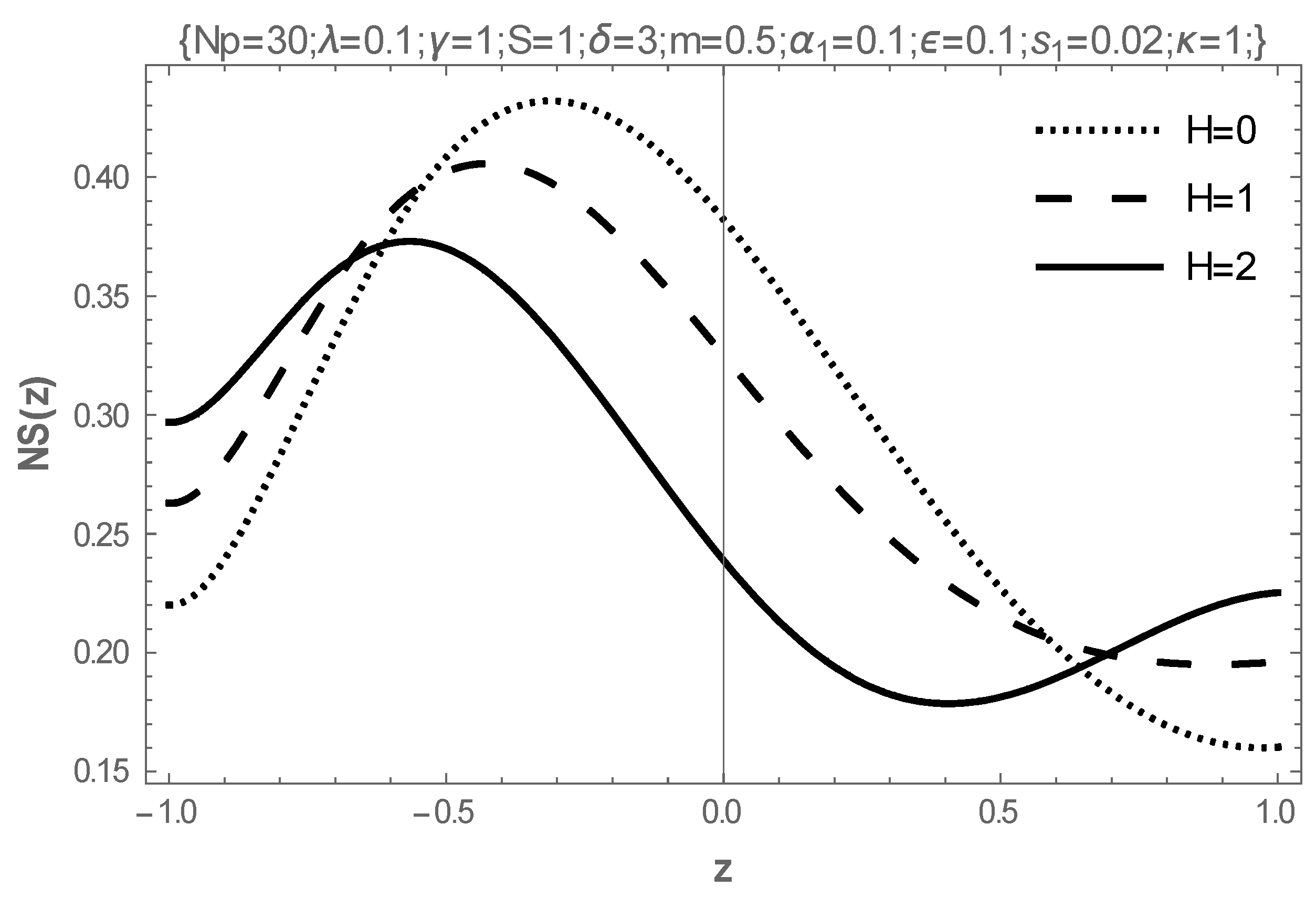
• The increasing values of the Hartmann number, electrokinetic width, electric field parameter, joule heat parameters, and the couple-stress parameter destabilize the flow, while the coefficient of viscosity and the activation energy parameter stabilize the flow.
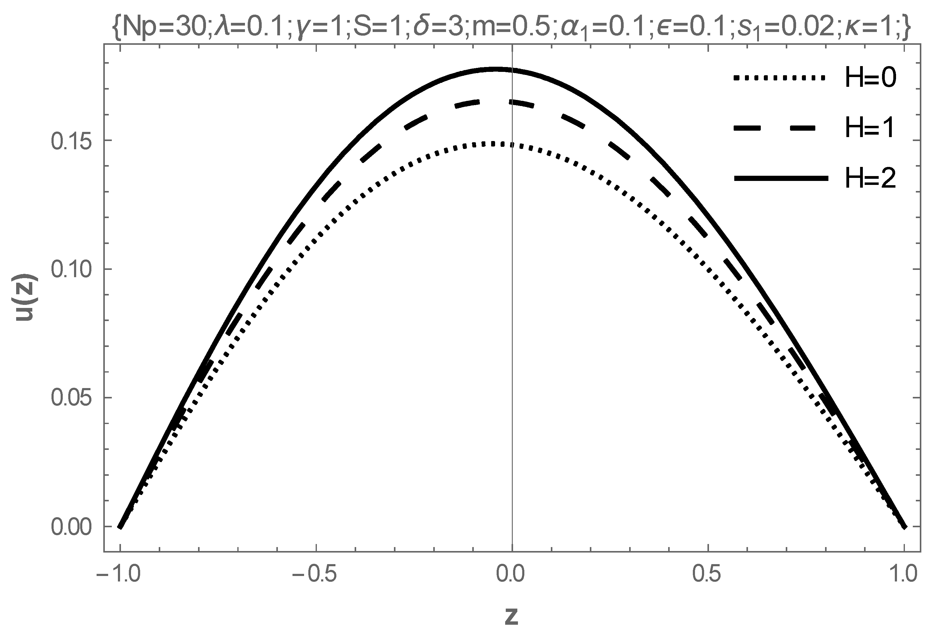
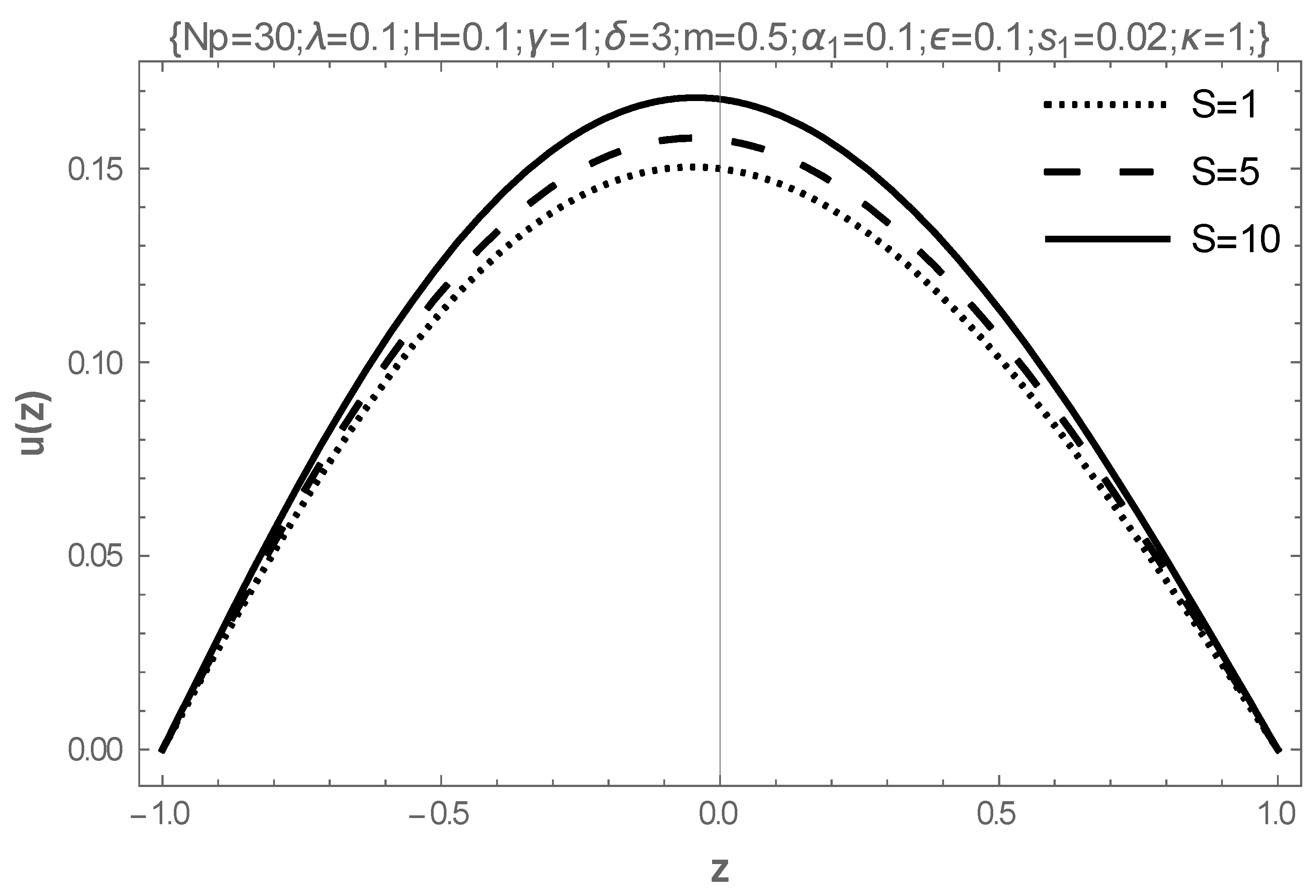
• The rising values of the Hartmann number, the coefficient of viscosity, and the electric field parameter enhance the flow of fluid, while the Frank-Kameneskii parameter does not have an effect on the flow velocity.
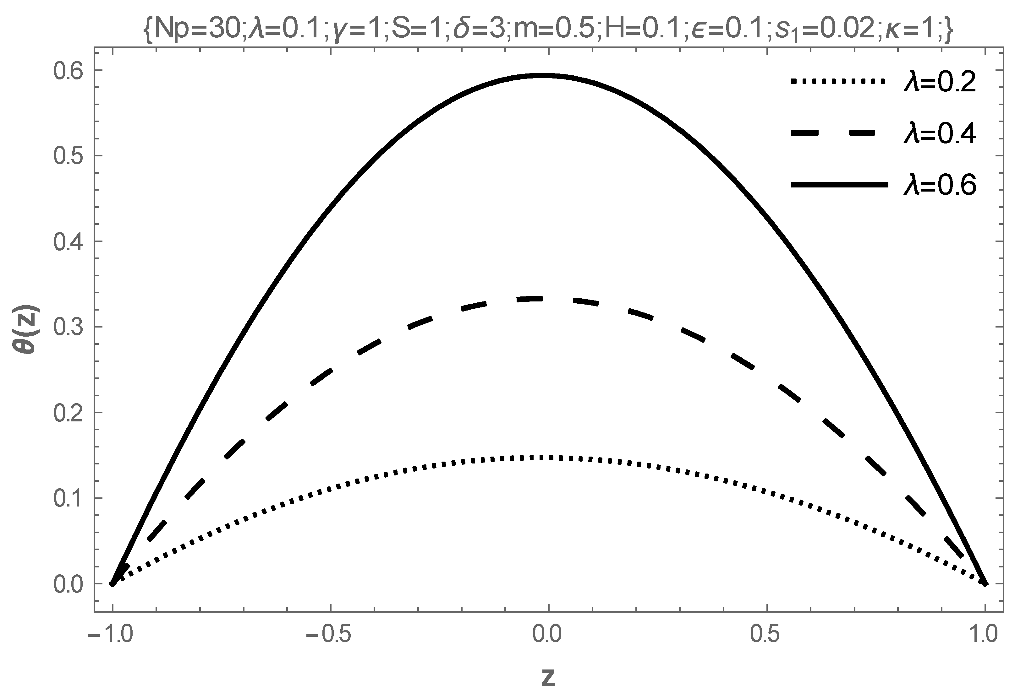
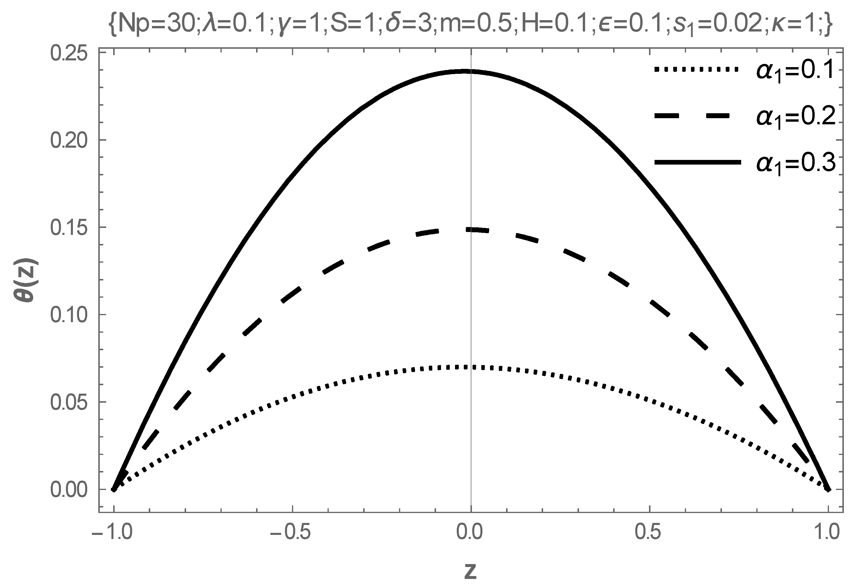
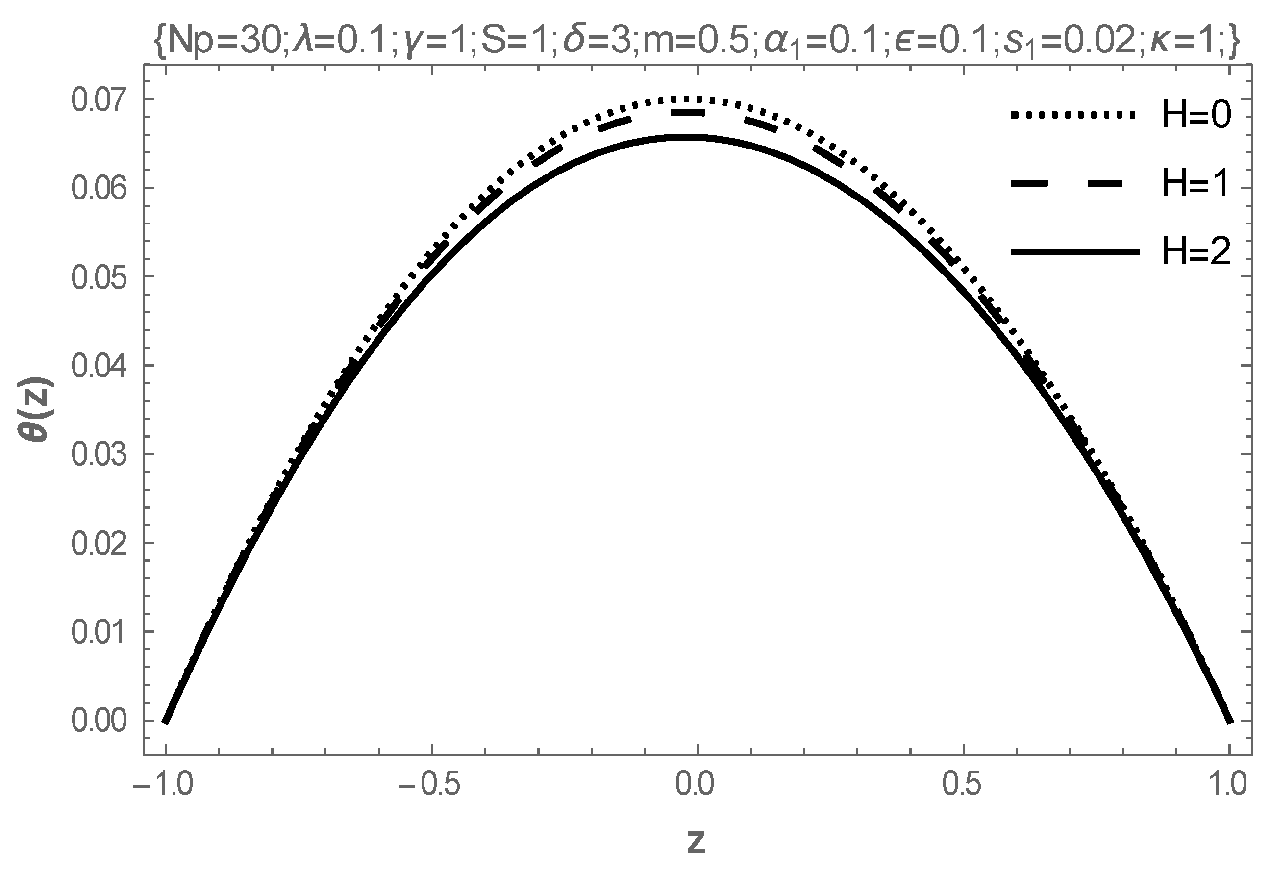
• In addition, intensifying the values of the Frank-Kameneskii parameter and the coefficient of viscosity elevates the temperature of the fluid, while the Hartmann number reduces the temperature.

The limitations of the model include the neglect of three-dimensional effects, convective cases, and other variable physical properties. This model is most applicable to small-scale systems where these assumptions hold true, such as microfluidic devices or controlled laboratory environments. It may require adjustments when applied to large-scale industrial processes or highly dynamic systems.

References

1. Elboughdiri, N.; Javid, K.; Shehzad, M.Q.; Benguerba, Y. Influence of chemical reaction on electro-osmotic flow of nanofluid through convergent multi-sinusoidal passages. Case Stud. Therm. Eng. 2024, 54, 103955. [Google Scholar] [CrossRef]
2. Reddy, M.G.; Reddy, K.V.; Souayeh, B.; Fayaz, H. Numerical entropy analysis of MHD electro-osmotic flow of peristaltic movement in a nanofluid. Heliyon 2024, 10, e27185. [Google Scholar] [CrossRef] [PubMed]
3. Tripathi, D.; Bhushan, S.; Beg, O.A. Unsteady viscous flow driven by the combined effects of peristalsis and electro-osmosis. Alex. Eng. J. 2018, 57, 1349–1359. [Google Scholar] [CrossRef]
4. Sakinder, S.; Salahuddin, T. A numerical study of electro-osmosis Williamson nanofluid flow in a permeable tapered channel. Alex. Eng. J. 2023, 81, 620–625. [Google Scholar] [CrossRef]
5. Nazeer, M.; Hussain, F.; Ghafar, M.M.; Javed, M.A. Investigation of electro-osmotic flow of Hafnium particles mixed-up with Casson fluid in convergent geometry: Theoretical study of multiphase flow. Partial. Differ. Equ. Appl. Math. 2022, 6, 100448. [Google Scholar] [CrossRef]
6. Abdul-Wahab, M.S.; Al-Saif, A.J. Studying the effects of electro-osmotic and several parameters on blood flow in stenotic arteries using CAGHPM. Partial. Differ. Equ. Appl. Math. 2024, 11, 100767. [Google Scholar] [CrossRef]
7. Siva, T.; Jangili, S.; Kumbhakar, B. Analytical solution to optimise the energy generation in EHMD flow of non-Newtonian fluid through a microchannel. Pramana J. Phys. 2022, 96, 168. [Google Scholar] [CrossRef]
8. Raju, U.; Rangabashyam, S.; Alhazmi, H.; Khan, I. Irreversible and reversible chemical reaction impacts on convective Maxwell fluid flow over a porous media with activation energy. Case Stud. Therm. Eng. 2024, 61, 104821. [Google Scholar] [CrossRef]
9. Tanveer, A.; Jarral, S.; Saleem, S. Dynamic interactions in MHD Jeffrey fluid: Exploring peristalsis; electro osmosis and homogeneous/heterogeneous chemical reactions. Alex. Eng. J. 2024, 94, 354–365. [Google Scholar] [CrossRef]
10. Prashanth, M.; Rao, V.S. The impact of soret, Dufour, and chemical reaction on MHD nanofluid over a stretching sheet. Partial. Differ. Equ. Appl. Math. 2024, 10, 100674. [Google Scholar] [CrossRef]
11. Vijayalakshmi, K.; Chandulal, A.; Alhazmi, H.; Aljohani, A.F.; Khan, I. Effect of chemical reaction and activation energy on Riga plate embedded in a permeable medium over a Maxwell fluid flow. Case Stud. Therm. Eng. 2024, 59, 104457. [Google Scholar] [CrossRef]
12. Iranian, D.; Karthik, S.; Seethalakshmy, A. Heat generation effects on Magnetohydrodynamic Powell-Eyring fluid flow along a vertical surface with a Chemical reaction. Forces Mech. 2023, 12, 100212. [Google Scholar] [CrossRef]
13. Adesanya, S.O.; Adeosun, A.T.; Lebelo, R.S.; Tisdell, C.C. Numerical investigation of reaction driven magneto-convective flow of Sisko fluid. Numer. Heat Transf. Part A Appl. 2024, 85, 1–14. [Google Scholar] [CrossRef]
14. He, Z.; Arain, M.B.; Usman; Khan, W.A.; Alzahrani, A.R.; Muhammad, T.; Hendy, A.S.; Ali, M.R. Theoretical exploration of heat transport in a stagnant power-law fluid flow over a stretching spinning porous disk filled with homogeneous-heterogeneous chemical reactions. Case Stud. Therm. Eng. 2023, 50, 103406. [Google Scholar] [CrossRef]
15. Prasad, K.V.; Vajravelu, K.; Datti, P.S. The effects of variable fluid properties on the hydro-magnetic flow and heat transfer over a non-linearly stretching sheet. Int. J. Therm. Sci. 2010, 49, 603–610. [Google Scholar] [CrossRef]
16. Adeyemo, A.S.; Sibanda, P.; Goqo, S.P. Analysis of heat and mass transfer of a non-linear convective heat generating fluid flow in a porous medium with variable viscosity. Sci. Afr. 2024, 24, e02140. [Google Scholar] [CrossRef]
17. Wu, Y.; Pruess, K. Integral solutions for transient fluid flow through a porous medium with pressure dependent permeability. Int. J. Rock Mech. Min. Sci. 2000, 37, 51–61. [Google Scholar] [CrossRef]
18. Jalili, B.; Azar, A.A.; Jalili, P.; Ganji, D.D. Impact of variable viscosity on asymmetric fluid flow through the expanding/contracting porous channel: A thermal analysis. Case Stud. Therm. Eng. 2023, 52, 103672. [Google Scholar] [CrossRef]
19. Obalalu, A.M.; Ajala, O.A.; Adeosun, A.T.; Akindele, A.O.; Oladapo, O.A.; Olajide, O.A.; Adegbite, P. Significance of variable electrical conductivity on non-Newtonian fluid flow between two vertical plates in the coexistence of Arrhenius energy and exothermic chemical reaction. Partial. Differ. Equ. Appl. Math. 2021, 4, 100184. [Google Scholar] [CrossRef]
20. Ramakrishna, O.; Falodun, B.O.; Akinremi, O.J.; Omole, E.O.; Ismail, A.S.; Amoyedo, F.E. Thermodynamics of variable thermophysical properties of non-Newtonian fluids with the exploration of antiviral and antibacterial mechanisms using silver nanoparticles. Int. J. Thermofluids 2024, 22, 100648. [Google Scholar] [CrossRef]
21. Sivaraj, R.; Kumar, B.R. Viscoelastic fluid flow over a moving vertical cone and flat plate with variable electric conductivity. Int. J. Heat Mass Transf. 2013, 61, 119–128. [Google Scholar] [CrossRef]
22. Adeosun, A.T.; Ukaegbu, J.C. Effect of the variable electrical conductivity on the thermal stability of the MHD reactive squeezed fluid flow through a channel by a spectral collocation approach. Partial. Differ. Equ. Appl. Math. 2022, 5, 100256. [Google Scholar] [CrossRef]
23. Salawu, S.O.; Obalalu, A.M.; Shamshuddin, M.D.; Fatunmbi, E.O.; Ajilore, O.J. Thermal stability of magneto-hybridized silicon and aluminum oxides nanoparticle in C3H8O2-Williamson exothermic reactive fluid with thin radiation for perovskite solar power. Kuwait J. Sci. 2024, 51, 100284. [Google Scholar] [CrossRef]
24. Adesanya, S.O.; Falade, J.A.; Ukaegbu, J.C.; Makinde, O.D. Adomian-Hermite-Padé approximation approach to thermal criticality for a reactive third grade fluid flow through porous medium. Theor. Appl. Mech. 2016, 43, 133–144. [Google Scholar] [CrossRef]
25. Alireza, N.; Javad, A.S.; Amin, S.N.; Hamidreza, H.; Majid, V. Influence of monoethanolamine on thermal stability of starch in water based drilling fluid system. Petrol. Explor. Develop. 2018, 45, 167–171. [Google Scholar]
26. Lebelo, R.S.; Mahlobo, R.K.; Adesanya, S.O. Reactant consumption and thermal decomposition analysis in a two-step combustible slab. Defect Diffus. Forum 2019, 393, 59–72. [Google Scholar] [CrossRef]
27. Doninelli, M.; Marcoberardino, G.D.; Alessandri, I.; Invernizzi, C.M.; Iora, P. Fluorobenzene as new working fluid for high-temperature heat pumps and organic Rankine cycles: Energy analysis and thermal stability test. Energy Convers. Manag. 2024, 321, 119023. [Google Scholar] [CrossRef]
28. Salawu, S.O.; Hassan, A.R.; Abolarinwa, A.; Oladejo, N.K. Thermal stability and entropy generation of unsteady reactive hydromagnetic Powell-Eyring fluid with variable electrical and thermal conductivities. Alex. Eng. J. 2019, 58, 519–529. [Google Scholar] [CrossRef]
29. Adesanya, S.O.; Banjo, P.O.; Lebelo, R.S. Exergy analysis for combustible third-grade fluid flow through a medium with variable electrical conductivity and porous permeability. Mathematics 2023, 11, 1882. [Google Scholar] [CrossRef]
30. Hoetink, A.E.; Faes, T.J.C.; Visser, K.R.; Heethaar, R.M. On the flow dependency of the electrical conductivity of blood. IEEE Trans. Bio-Med. Eng. 2004, 51, 1251–1261. [Google Scholar] [CrossRef] [PubMed]
31. Khan, A.; Farooq, M.; Nawaz, R.; Ayaz, M.; Ahmad, H.; Abu-Zinadah, H.; Chu, Y.M. Analysis of couple stress fluid flow with variable viscosity using two homotopy-based methods. Open Phys. 2021, 19, 134–145. [Google Scholar] [CrossRef]
32. Baranovskii, E.S.; Prosviryakov, E.Y.; Ershkov, S.V. Mathematical analysis of steady non-isothermal flows of a micropolar fluid. Nonlinear Anal. Real World Appl. 2025, 84, 104294. [Google Scholar] [CrossRef]
33. Baranovskii, E.S.; Ershkov, S.V.; Prosviryakov, E.Y.; Yudin, A.V. Exact solutions to the Oberbeck-Boussinesq equations for describing three-dimensional flows of micropolar liquids. Symmetry 2024, 16, 1669. [Google Scholar] [CrossRef]
Figure 1. Flow geometry.
Mathematics 13 00615 g001
Figure 2. Effect of chemical reactions on the velocity profile.
Mathematics 13 00615 g002
Figure 3. Effect of chemical reactions on temperature distribution.
Mathematics 13 00615 g003
Figure 4. Effect of chemical reactions on entropy generation.
Mathematics 13 00615 g004
Figure 5. Effect of chemical reactions on Bejan number.
Mathematics 13 00615 g005
Figure 6. Effect of variable viscosity on velocity profile.
Mathematics 13 00615 g006
Figure 7. Effect of variable viscosity on temperature distribution.
Mathematics 13 00615 g007
Figure 8. Effect of variable viscosity on entropy generation.
Mathematics 13 00615 g008
Figure 9. Effect of variable viscosity on Bejan number.
Mathematics 13 00615 g009
Figure 10. Effect of Hartmann number on the velocity profile.
Mathematics 13 00615 g010
Figure 11. Effect of the Hartmann number on the temperature distribution.
Mathematics 13 00615 g011
Figure 12. Effect of the Hartmann number on entropy generation.
Mathematics 13 00615 g012
Figure 13. Effect of Hartmann number on Bejan number.
Mathematics 13 00615 g013
Figure 14. Effect of electric field parameter on the velocity profile.
Mathematics 13 00615 g014
Figure 15. Effect of electric field parameter on temperature distribution.
Mathematics 13 00615 g015
Figure 16. Effect of electric field parameter on entropy generation.
Mathematics 13 00615 g016
Figure 17. Effect of electric field parameter on Bejan number.
Mathematics 13 00615 g017
Figure 18. Thermal criticality.
Mathematics 13 00615 g018