Article

Golden Ratio Function: Similarity Fields in the Vector Space

by
Artyom Grigoryan
1,* and
Meruzhan Grigoryan
2
1
Department of Electrical and Computer Engineering, The University of Texas at San Antonio, San Antonio, TX 78249, USA
2
Faculty of Physics, The Yerevan State University, Yerevan 0025, Armenia
*
Author to whom correspondence should be addressed.
Mathematics 2025, 13(5), 699; https://doi.org/10.3390/math13050699
Submission received: 20 January 2025 / Revised: 15 February 2025 / Accepted: 17 February 2025 / Published: 21 February 2025

Abstract

:
In this work, we generalize and describe the golden ratio in multi-dimensional vector spaces. We also introduce the concept of the law of similarity for multidimensional vectors. Initially, the law of similarity was derived for one-dimensional vectors. Although it operated with the values of the ratio of the parts of the whole, it created linear dimensions (a line is one-dimensional). The presented concept of the general golden ratio (GGR) for the vectors in a multidimensional space is described in detail with equations. It is shown that the GGR is a function of one or more angles, which is the solution to the golden equation described in this work. The main properties of the GGR are described, with illustrative examples. We introduce and discuss the concept of the golden pair of vectors, as well as the concept of a set of similarities for a given vector. We present our vision on the theory of the golden ratio for triangles and describe similarity triangles in detail and with illustrative examples.

1. Introduction

The golden ratio, or the famous number Φ = 1.6180 , is also known as the divine proportion between two quantities [1,2,3]. The concept of division in the mean and extreme ratio, or the golden ratio, was introduced into scientific circulation by Pythagoras (6th century BC), and many ancient Greek philosophers and mathematicians have studied it. Golden proportions are present in the facade of the ancient Greek temple of Parthenon. Plato also knew about the golden division. Plato’s dialogue, “Timaeus” (360 BC), is devoted, in particular, to issues of the golden division. Apparently, Pythagoras borrowed his knowledge of the golden division from the Egyptians and Babylonians [4,5]. The number Φ has been found in the proportions of some parts of the construction of Egyptian pyramids [6], in arts [7,8,9], fashion [10], medicine [11,12], face detection [13], image enhancement [14,15], colors of paintings [16], and has many applications in engineering.
The illustration of the golden ratio rule is given in Figure 1. Assuming the lengths b > a > 0 , the interval of length l = a + b is divided in the mean proportional relation ( b + a ) / b = b / a = Φ .
There are many geometric figures that can be described by proportions related to the number Φ . As an example, the well-known isosceles triangle, with angles of 72 ° , 72 ° , and 36 ° , has been considered as the golden triangle [4]. Fifteen similar triangles are found in a figure composed of a circle with an inscribed pentagon and a five-pointed star, or pentagram, which are shown in Figure 2a. One of these golden triangles is shown in part (b). In this triangle, the ratio of the larger side to the smaller side is the golden number Φ . It is also known that, if we inscribe a regular decagon on the unit circle in Figure 2a, the side of the decagon will have a length of 1 / Φ = 0.6180   [5].
The right triangle, with its properties shown in Figure 3a, is another example of the golden triangle. Such a triangle can be seen in the construction of the ancient Cheops pyramid [2]. As shown in the figure, the ratio of the hypotenuse, x , to the biggest side, h , of the triangle is the square root of the golden ratio, Φ . The ratio of the hypotenuse to the smallest side, y , of the triangle is Ψ . The vertical cross-section of the pyramid of Cheops is illustrated in part (b). The length of the base of the triangle is 230.33 m and the height, h , is 146.60 m (according to the original data). The slope of this equilateral triangle is 51.8478 ° . It should be noted that the height of the golden right triangle, whose base is exactly 230.33 m, must be 146.94 m, which is very close to 146.60 m.
In this work, we generalize and describe the golden ratio in multi-dimensional vector spaces. We present for the first time the concept of a general golden ration (GGR) that depends on the direction in the space. Many examples of vectors in golden ratios are described in detail in two-, three-, and six-dimensional spaces. The main contributions of this work can be summarized as follows:
  • The concept of the golden ratio has generalization in the multi-dimensional vector space;
  • The general golden ratio is a function of one or more angles, and this is one of four solutions to the golden equation presented here;
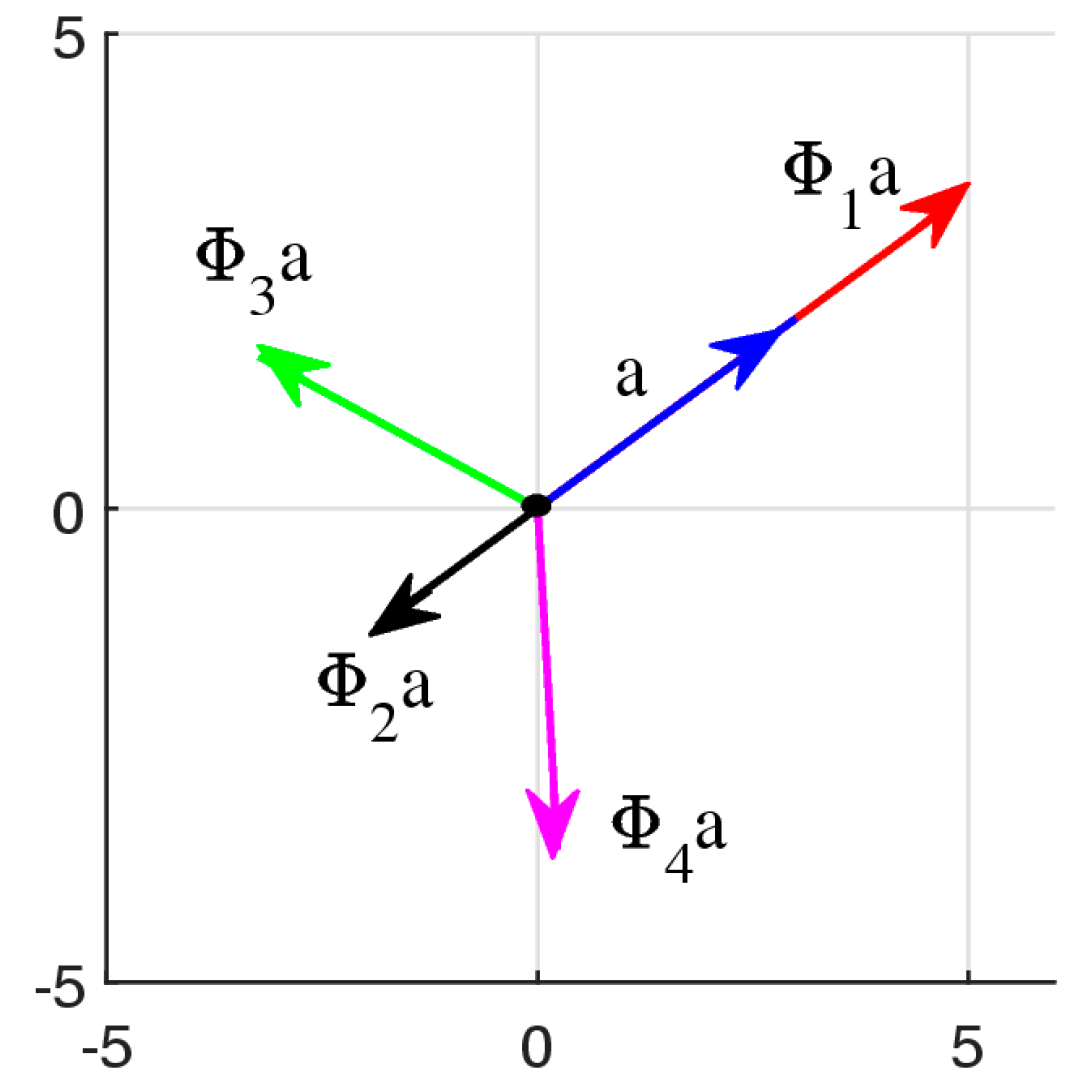
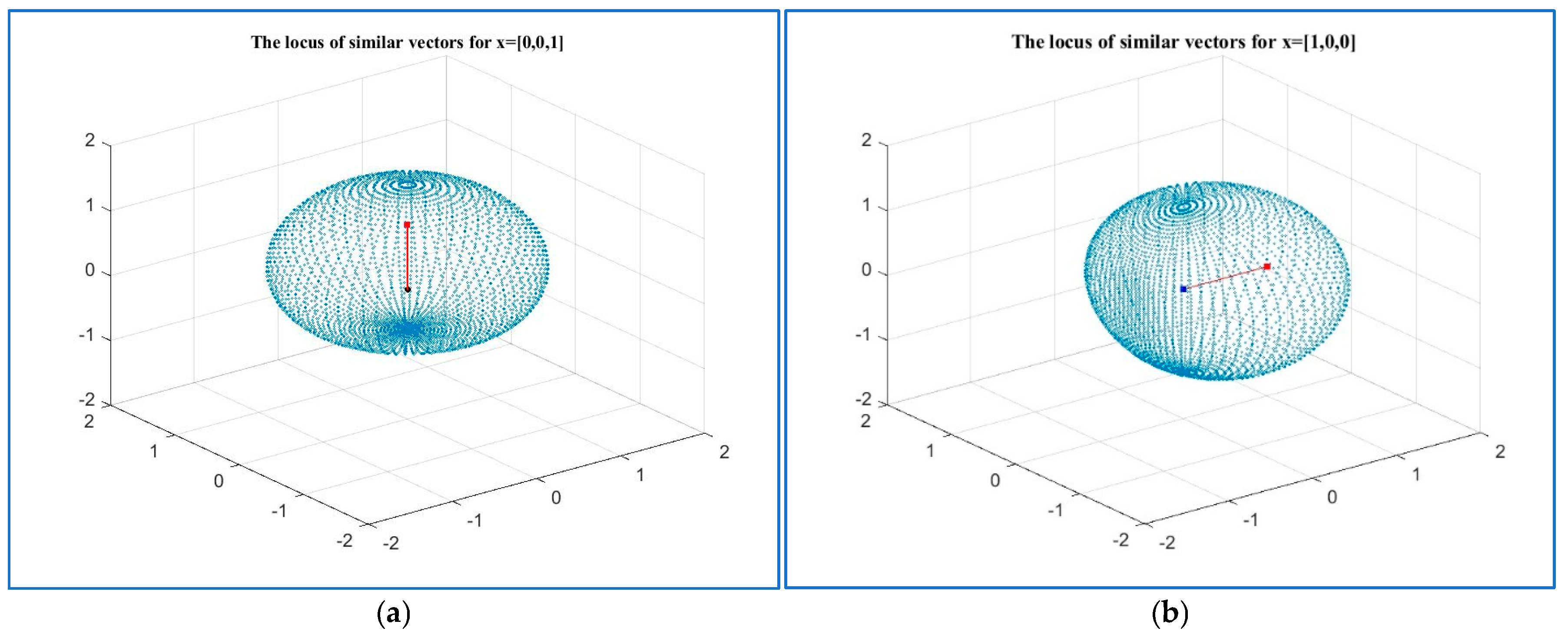
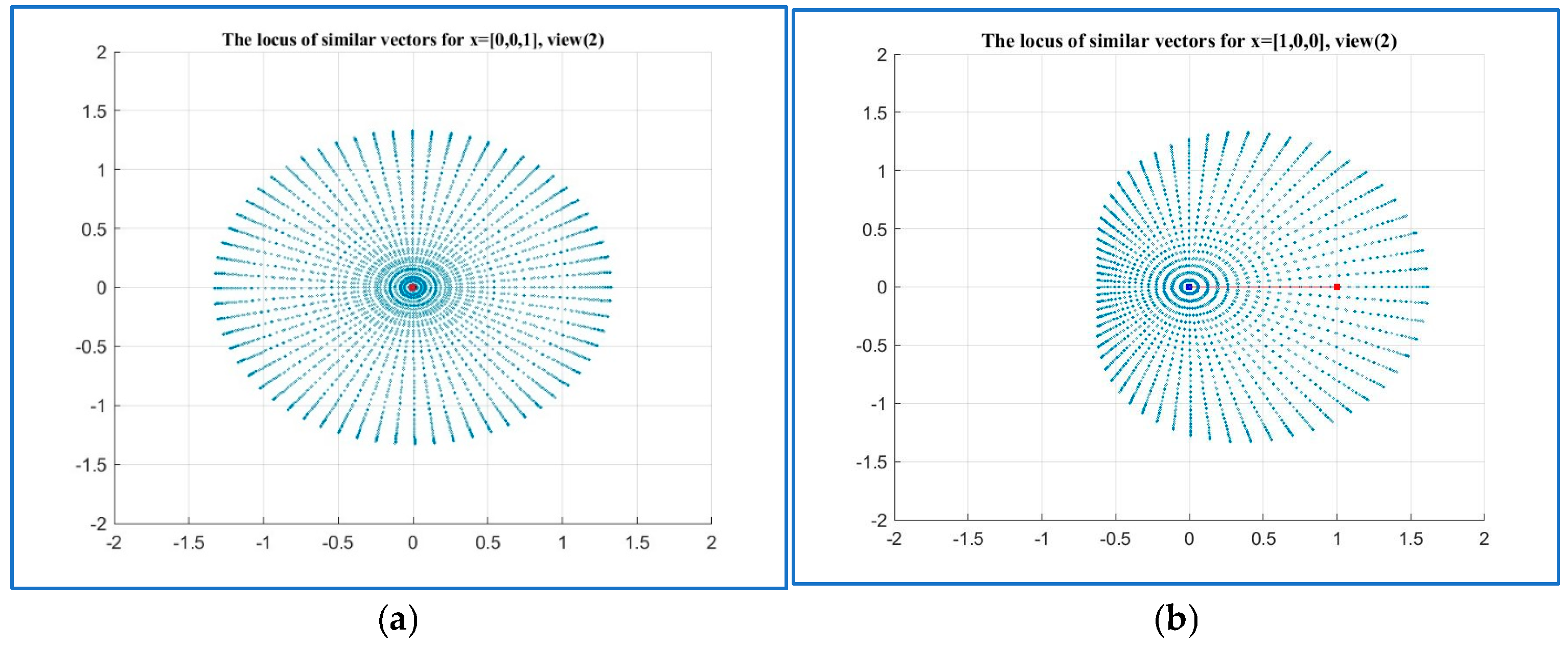
  • Each vector v in space corresponds to a set of similarities or a set of vectors in the golden ratio with v ;
  • GGR can be used to describe similar figures, such as a vector space of triangles;
  • Each vector affects its environment, exerting its influence through the imposition of its likeness or similarities;
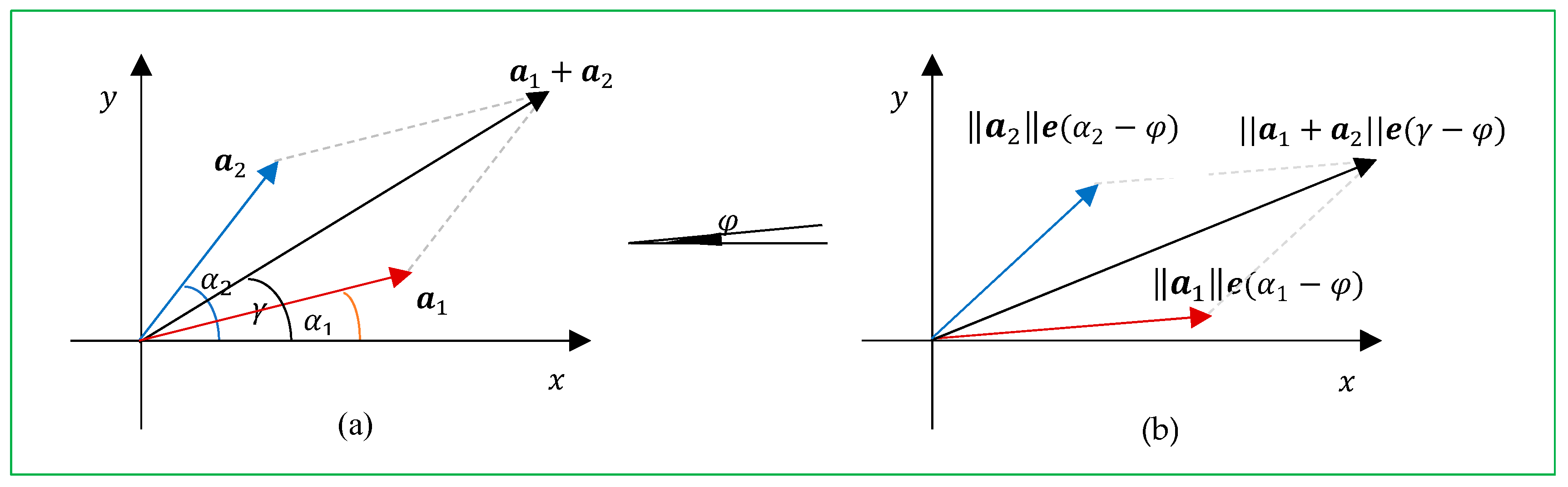
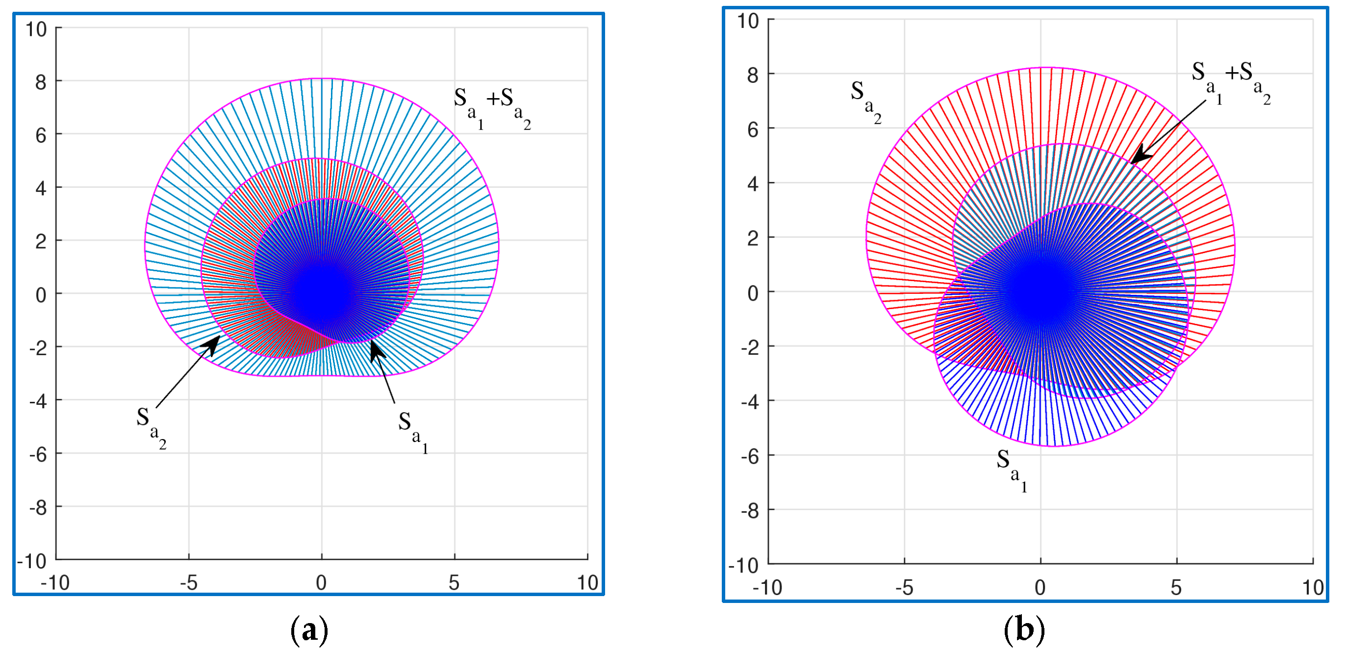
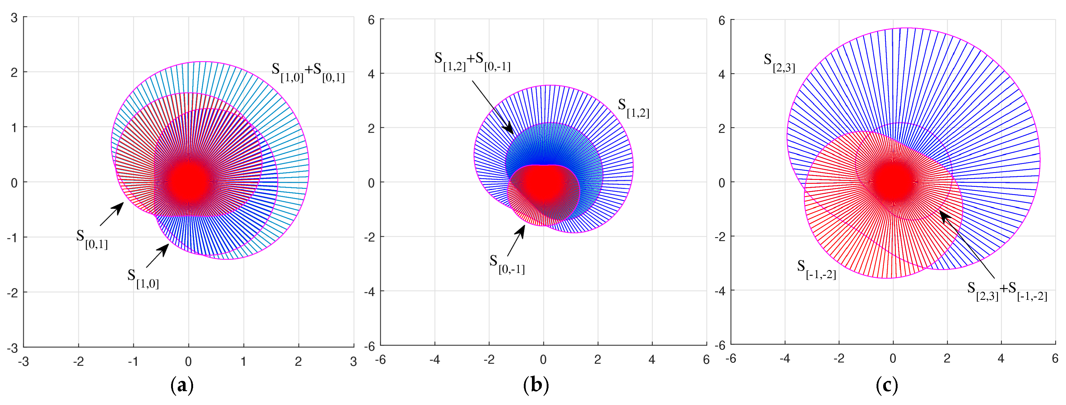
  • The sets of similarities of vectors can be summed.
The rest of the paper is organized in the following way. Section 2 presents the definition of the general golden ratio in the vector space. The main equation of the GGR and its solutions are described in Section 3. The golden ratio in the two-dimensional (2D) space, with examples, is considered in Section 4. In Section 5, the concept of vector similarity sets is presented and described, with examples in 2D and three-dimensional (3D) spaces. The vector space of triangles and golden ratio of triangles are described in detail in Section 6. Illustrative examples are given. In Section 7, similarity figures are described with many examples, including the pentagon, heptagon, the seven- and nine-pointed stars, and Archimedes’ spiral.

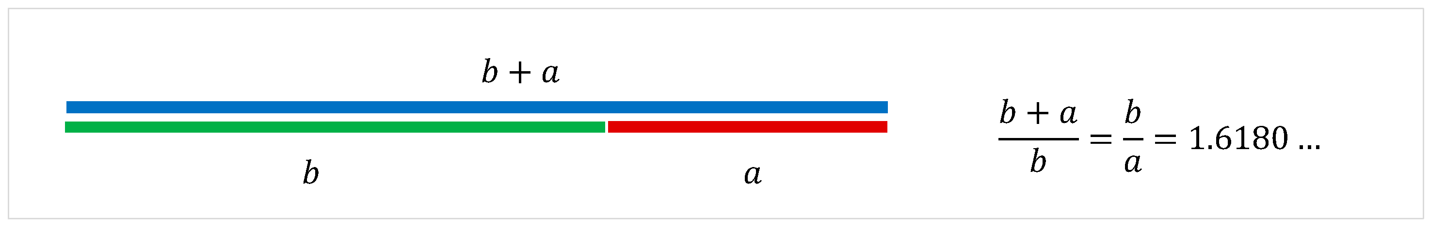
2. The Generalized Golden Ratio (GGR)

In this section, we extend the well-known concept of the gold ratio in an n -dimension vector space, when n 1 . Let V be a normed vector space over real numbers λ . This means that there exists such a real-valued function as l : V R , which is denoted by l x = x , and that the following properties hold:
  • x 0 , and x = 0 means that x = 0 ;
  • λ x = | λ | x , for any real number λ R ;
  • x + y x + y , for any elements x and y V .
The function x is called the length, or the norm, of the element x .
Definition 1.
In a normed vector space  V , the function f : V × V R , which satisfies the following conditions:
  • f a , b 0 , for any elements  a  and  b V ;
  • If  a = 0 ,   f 0 , b = 0 ;
  • If  b 0 ,   f a , b ;
  • For any real number,  λ R , f λ a , λ b = f a , b
is called the proportion.
As an example, when  V = R , the function  f a , b = a / | b |  is a proportion. This is the function that interests us the most.
Definition 2.
Given the proportion  f : V × V R   in the normed vector space V , two elements, a   and b V , are called the golden pair, if the following equality holds:
f b + a , b = f a , b .
The elements   a   and   b   are also called the golden ratio elements relative to the proportion  f . We call Equation (1) the golden ratio equation.
Definition 3.
If elements  a   and b   are golden ratio elements relative to a proportion f ,  then the ratio Φ = a / b  is called the generalized golden ratio, or, shortly, the GGR.
In the example below for the 1D vector space, this number is the known golden ratio [1]. Therefore, we use a similar name in the n-dimensional space. So as not to underestimate the historical nature of this number, we added a generalized meaning.
Example 1.
Let V = R and the function  f a , b = a / | b |  be the proportion.Here, we consider that a = a for real numbers. To find the golden ratio elements a and b , we consider primary Equation (1):
| b + a | | b | = | b | | a | ,       o r      | b + a | | a | = | b | 2 | a | 2 .
It can be written as
| b | | a | 2 = | b + a | | a | = | b | | a | b | b | + a | a | ,
or
Φ 2 = Φ + s i g n ( a b ) .
Here, the function   s i g n a b = 1 , if   a b > 0 , and   s i g n a b = 1 , if   a b < 0 . The case   a = 0   or   b = 0   is not considered.
The solutions of this equation are considered for the following two possible cases.
  • Case Φ + s i g n ( a b ) 0 : the equation to be solved is
    Φ 2 Φ s i g n a b = 0 .  
    The solutions are
    Φ 1,2 = 1 ± 1 + 4   s i g n ( a b ) 2 .
    Such numbers are real only when s i g n a b = 1 ; that is, the angle between the elements a and b is α = 0 . Therefore,
    Φ 1 = 1 + 5 2 = 1.6180339887 ,         Φ 2 = 1 5 2 = 0.6180339887   .  
    A golden ratio is a positive number. The first number Φ 1 is considered, but the second number Φ 2 is not considered, since it is negative. Thus, the golden ratio is Φ 0 = Φ 1 .
2.
Case Φ + s i g n a b < 0 : The following equation is considered:
Φ 2 + Φ + s i g n a b = 0
with the solutions
Φ 1,2 = 1 ± 1 4   s i g n ( a b ) 2 .
Such numbers are real only when s i g n a b = 1 ; that is, the angle between the elements a and b is α = π . Therefore,
Φ 1 = 1 + 5 2 = 0.6180 ,         Φ 2 = 1 5 2 = 1.6180   .  
Here, Φ 2 is negative and the solution Φ π = Φ 1 is considered, since the condition of consideration is not violated; that is, Φ 1 + s i g n a b = Φ 1 1 = 0.3819 < 0 . Thus, a golden pair can be composed from numbers of opposite signs. This example shows that for any number a 0 , there are two numbers that compose the golden ratio with a . These numbers have different signs and are equal to a Φ 0 and a Φ π . The golden pairs are the ordered pairs { a , a Φ 0 } and { a , a Φ π } . In the 1D space R , when setting the system of coordinates, we match each point to a certain number, implying by this number a certain measure of distance from the center of coordinates. Therefore, in the 1D case, we deal with linear objects (segments on the real line R ) which have the length, and this is exactly the value we obtained for a certain proportion called the golden ratio. Two linear objects are in the golden ratio if the ratio of their measures (lengths) is equal to the number Φ = Φ 0 or Φ π = Φ 0 1 .
We will try to transfer the idea of the golden ratio into the 2D plane (with 1D and 2D objects), considering the starting point 0 in a given system of coordinates. Before we start to work with equations, we need to prepare ourselves for all possible results and develop the ability to explain them. The point is that 2D objects include 1D objects, and the golden ratio rule must remain unchanged for them. Let us consider a vector x 1 and the corresponding similar vector x 2 = Φ x 1 (see Figure 4 in part (a)). It can be noted that the 2D measures of the similar vectors x 1 and x 2 or the areas of their shadows are in the ratio Φ 2 , not in Φ .
We consider that two vectors x 1 and y 1 compose a figure; for instance, a 2D object, such as a parallelogram, P 1 , as shown in part (b). Thus, these vectors are related; this relationship depends on the angle between these vectors. Then, the question arises of how the proportions of these 2D objects cannot depend on the connectedness of vectors. In the general case, this number, or the ratio, is the function of the angle, which we denote by Φ 2 D φ .   When the angle between the vectors is zero, the 2D object is a line. Therefore, in order for the 1D golden ratio to manifest itself, it is necessary to request the condition Φ 2 D ( 0 ) = Φ . Note that instead of the parallelograms, we can also consider other figures, including the triangles composed by these vectors, as shown in part (c). Now, we will describe in detail the concept of the golden ratio in a multi-dimensional vector space.
Example 2.
Consider the  n -dimensional vector space  V = R n ,   n > 1 . It is not difficult to show that the function
f a , b = a b ,     a , b V ,     b 0 ,     
is the proportion. Here, the norms   a = a 1 2 + a 2 2 + + a n 2  and   b = b 1 2 + b 2 2 + + b n 2 .
We consider the golden ratio equation (rule) f b + a , b = f a , b written as
b + a b = b a ,    o r      b + a a = b 2 .
The following calculations are valid for this equation:
a 2 + b 2 + 2 a , b   a = b 2 , a 2 + b 2 + 2 a b c o s ( α )   a = b 2 , 1 + b 2 a 2 + 2 b a cos α = b 4 a 4 .
Here, a , b is the inner product in the space V , and α is the angle between the vectors a and b . Denoting the golden ratio by x = Φ = b / a , we obtain the equation 1 + x 2 + 2 x cos ( α ) = x 4 ,   or
x 4 x 2 2 x cos α 1 = 0 .  
This equation has four roots, x n = x n ( α ) and n = 1 : 4 , which are functions of the angle α . Thus, the GGR depends on the angle. Since cos α = cos 2 π α , the roots x n ( 2 π α ) =   x n ( α ) for α 0 , π . Also, x n ( π + α ) = x n ( α ) .
A. Case α = 0 (vectors are collinear or they are in the same directions): The equation x 4 x 2 2 x 1 = 0 can be written as
x 4 x 2 2 x 1 = x 2 x 1 x 2 + x + 1 = 0 .  
Therefore, we consider the solutions of the equation x 2 x 1 = 0 , which are
x 1,2   = 1 ± 5 2 = Φ 1,2   .
The positive solution is x 1 = Φ 1 = 1.6180 . Given vector a , the golden pair of vectors { a , a Φ 1 } are in the same direction, and the pair of vectors { a , a Φ 2 } are in the opposite direction. The second equation x 2 + x + 1 = 0 has two complex roots, namely
x 3,4   = 1 ± i 3 2 = e ± i 2 π 3 = Φ 3,4   .  
These complex coefficients of “similarity” are equal in absolute value to 1; that is, they do not affect the length, but only the rotation by ± 2 π / 3 . We can say that the first equation in Equation (7) defines similarity by length and the second equation defines similarity by rotation.
As an example, Figure 5 shows the 2D vector a = [ 3,2 ] at an angle of α = atan 2 / 3 = 33.6901 ° to the horizontal line, and four vectors a k = Φ k a ,   k = 1 : 4 .
It is not difficult to see that a 1 + a 2 = a and a 1 + a 2 + a 3 + a 4 = 0 . These equations hold for any vector a . The above figure illustrates the concept of similarity of the vector a or similarity by the angle α . Among these fours vectors, only the first one, a 1 = Φ 1 a , is in the golden ratio with a .
B. Case α = π / 2 (vectors are perpendicular): The equation x 4 x 2 1 = 0 is reduced to two equations:
x 2 = 1 + 5 2      a n d    x 2 = 1 5 2 .
Therefore, the first equation is considered, and its two solutions are
x 1,2   = ± 1 + 5 2 = ± Φ 1 = ± 1.6180339887   .  
The positive solution is x 1 = Φ 1 = 1.2720196495   . The solutions of the equation x 2 = ( 1 5 ) / 2 are the complex numbers
x 3,4   = ± i 5 1 2 = ± i Φ 2 = ± i 0.6180339887 = ± i 0.7861513775     .    
C. Case α = π (vectors are collinear in the opposite directions): The equation x 4 x 2 + 2 x 1 = 0 can be written as
x 4 x 2 + 2 x 1 = ( x 2 + x 1 ) ( x 2 x + 1 ) = 0 .
The solutions of the equation x 2 x + 1 = 0 are the complex numbers ( 1 ± i 3 ) / 2 . Therefore, we consider the solution of the equation x 2 + x 1 = 0 , which are (see Equation (4))
x 1   = 1 5 2 = Φ 1 ,     x 2   = 1 + 5 2 = Φ 2 = 0.6180339887   .
The positive solution is x 2 = Φ 2 . Thus, in the n -dimensional space, when n > 1 , two vectors in the opposite directions can form a golden pair.
D. Case x = 1 (the vectors of the golden pair have the same length): Equation (6) is 2 cos α + 1 = 0 and the angles α = 180 ± 60 . Two pairs of vectors with the angles α = 240 and 120 (in degrees) between them form the golden pairs when their lengths are equal. Figure 6 shows three vectors, a 1 , a 2 , and a 3 , with the same length. Each of these vectors are in the golden ratio with two others.

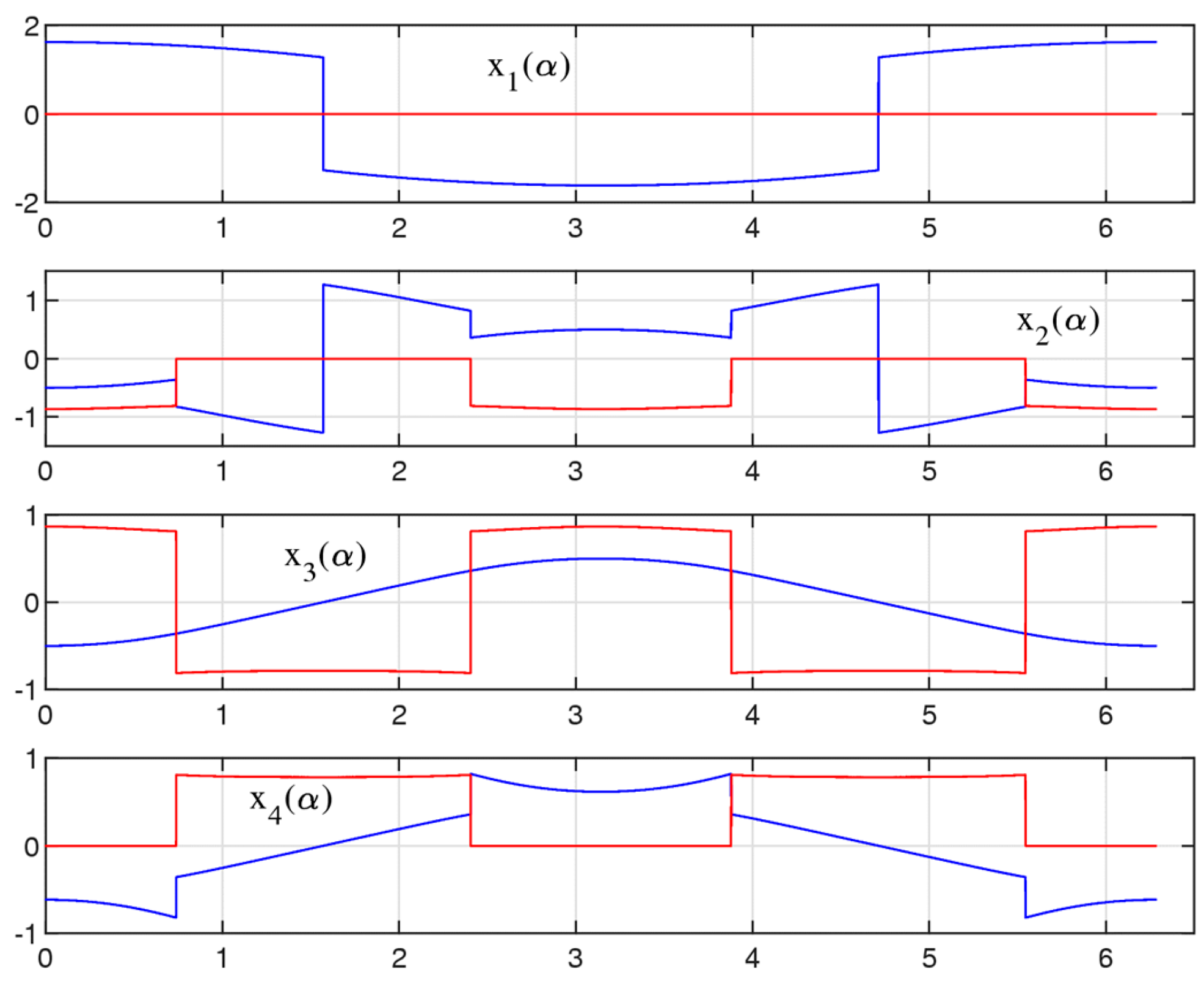
3. Main Equation of Golden Ratio and Its Analytical Solution

In this section, we describe the real roots of Equation (6), where x   is a function of the angle x = x α . The equation is
x 4 a x 2 a 2 cos α x α 1 = 0  
with the initial condition x 0 = 1.61803398… For each angle α, the quartic polynomial in this equation has four roots, and two of them are complex, therefore being a complex conjugate. We are looking for a positive solution of this equation, which should be only one. Equation (9) can be written as x 4 x 2 1 = 2 cos α x . The parabola P ( x ) = x 2 2 x 2 1 crosses the straight line with the slope 2 cos ( α ) at two points. As an illustration, Figure 7 shows the graph of the polynomial P ( x ) together with the line 2 cos ( α ) x , when α = 45 ° in part (a) and α = 100 ° in part (b).
For the angle α = 45 ° , the solutions of Equation (9) are
x 1 = 0.8492 ,      x 2 = 1.5325 ,      x 3 = 0.3416     0.8072 i ,      x 4 = x ¯ 3 = 0.3416 + 0.8072 i .  
The numbers are written with a decimal precision of four. At points x 1 and x 2 , the parabola P ( x ) = x 2 2 x 2 1 crosses the straight line y = 2 x , as shown in part (a). The second coordinate is positive. Thus, the required root is Φ = x 45 ° = 1.5325123089
For the angle α = 100 ° , the solutions of Equation (9) are
x 1 = 1.3455 ,     x 2 = 1.1894 ,     x 3 = 0.0780 + 0.7865 i ,     x 4 = x ¯ 3 = 0.0780     0.7865 i .  
The parabola P(x) crosses the straight line y = 2 cos ( 100 ° ) x at the point x 1 < 0 and the positive point x 2 . Therefore, Φ = x ( 100 ° ) = 1.1894 638778…
The case with the angle α = 30 ° (when Φ = x ( 30 ° ) = 1.5800943659 …) is shown in Figure 7c. Here, two lines ± 2 x are also shown (in red) as boundary lines y = ± 2 x for the lines y = 2 cos ( α ) x , when α π ,   π . It is clear that all these lines y intersect the parabola at two points, one of which is positive and the other is negative.

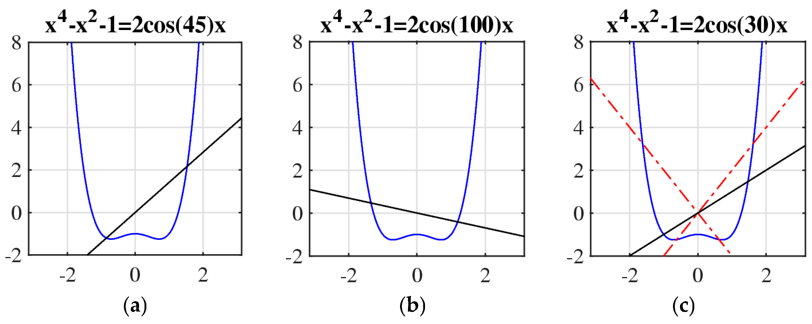
3.1. Similarity Equation and Its Roots

Consider again the gold ratio equation:
P 4 x = x 4 x 2 2 x cos ( α ) 1 = 0 .
We call the continuous roots of this equation the similarity functions and denote them by the symbols x k ( α ) , k 1 : 4 . The analytical exact solution of this quartic equation is very complicated [15,16,17,18]. The standard procedure is to add an auxiliary parameter t 0   to the quartic equation P 4 x = 0 , which can be written as
P 4 x = x 2 1 2 + t   2 2 t x 2 2 cos α x + t 2 t + 5 4 = 0 ,  
and then to request for a square polynomial in square brackets to be a square; that is,
P 2 x = 2 t x 2 2 cos α x + t 2 t + 5 4 = 2 t x y 1 2 .  
To have such a multiple root y 1 , the discriminant of the equation must be zero:
D 3 ( t ) = t 3 t 2 + 5 4 t 1 2 cos 2 α = 0 .   
Then, y 1 = cos α / ( 2 t ) , and the above quartic equation can be written as
P 4 x = 2 t x 2 1 2 + t   2 t ( x y 1 ) x 2 1 2 + t   + 2 t ( x y 1 ) = 0 .
The positive solution of this equation is one of the solutions of the quadratic equations:
x 2 1 2 + t   2 t ( x y 1 ) = 0      a n d   x 2 1 2 + t   + 2 t ( x y 1 ) = 0 .  
Cubic Equation (12) can be reduced to the following depressed cubic equation:
D 3 t D 3 v = v 3 + 11 12 v + 37 108 1 2 cos 2 α = 0 ,  
by changing the variable, t v , as t = v + 1 / 3 . Ferrari’s solution [19] to this equation states that it has a real root, if the following function is positive:
D α = 1 4   37 108 1 2 cos 2 α 2 + 1 27 11 12 2 .  
Figure 8 shows the graph of this polynomial   D α , α ( π , π ) , in part (a); it is positive. Therefore, the solution of Equation (15) is
v α = 1 2 q α + D α 3 + 1 2 q α D α 3 ,        q α = 37 108 1 2 cos 2 α .       
The graph of this function is shown in part (b). The positive function t α = v α + 1 / 3 can be used to solve two quadratic equations in Equation (14),
x 2 b 1 x + c 1 = 0      a n d      x 2 + b 1 x + c 2 = 0 ,   
which will give us four solutions, x k α ,   k = 1 : 4 . Here, the coefficients are calculated by
b 1 = 2 v α + 1 / 3   ,     c 1 = v α 1 / 6 + cos α / 2 v α + 1 / 3 , c 2 = v α 1 / 6 cos α / 2 v α + 1 / 3 .
It is clear that the formulas for solving the gold equation are cumbersome and difficult to visualize. Therefore, we consider another approach to describing solutions—using simple computer programs.
To analyze the equation of the generalized golden ratio, we compute its roots. Figure 9 shows the graphs of four roots x n ( α ) , n = 1 : 4 , of this equation. The real and imaginary parts of the roots are shown in blue and red colors, respectively. The angles α are in the interval [ 0,2 π ] with step 0.0015 radians, or 1/12 degrees. These roots were calculated using the command x=roots([1,0,−1,−2 cos(a),−1])’, by using the MATLAB R2022b function ‘roots.m’.
The graphs of the roots are symmetric about the vertical axis at angle point α = π . In some parts, these functions change sign. For example, the sign of the real part of the first solution x 1 ( α ) changes at angles π / 2 and 3 π / 2 and the jump is equal to 2 Φ 1 = 2 × 1.2720 . For other roots, the discontinuities can be seen at angle points π / 2 ± π / 4 and 3 π / 2   ± π / 2 . As shown in Equations (10)–(17) (see also Figure 8), the analytical solutions (not the ones that were computer generated) should not have points of discontinuity.
In Figure 10, these four roots are plotted in the polar form. The first plot is like the apple, the second a four-petal flower, the third an egg (Earth), and the fourth plot is a non-specific shape.
It is not difficult to note that the following holds for the roots of the above equation: x 1 α + x 2 α + x 3 α + x 4 α = 0 . Thus, x 4 α is equal to the sum of the first three roots with a minus sign. The fourth plot is the sum x 1 α + x 2 α + x 3 ( α ) in the polar form. Figure 11 shows the polar plots of the sums of roots x 1 α + x 2 α , x 2 α + x 3 α , and x 1 α + x 3 ( α ) in parts (a), (b), and (c), respectively. These figures are interesting.

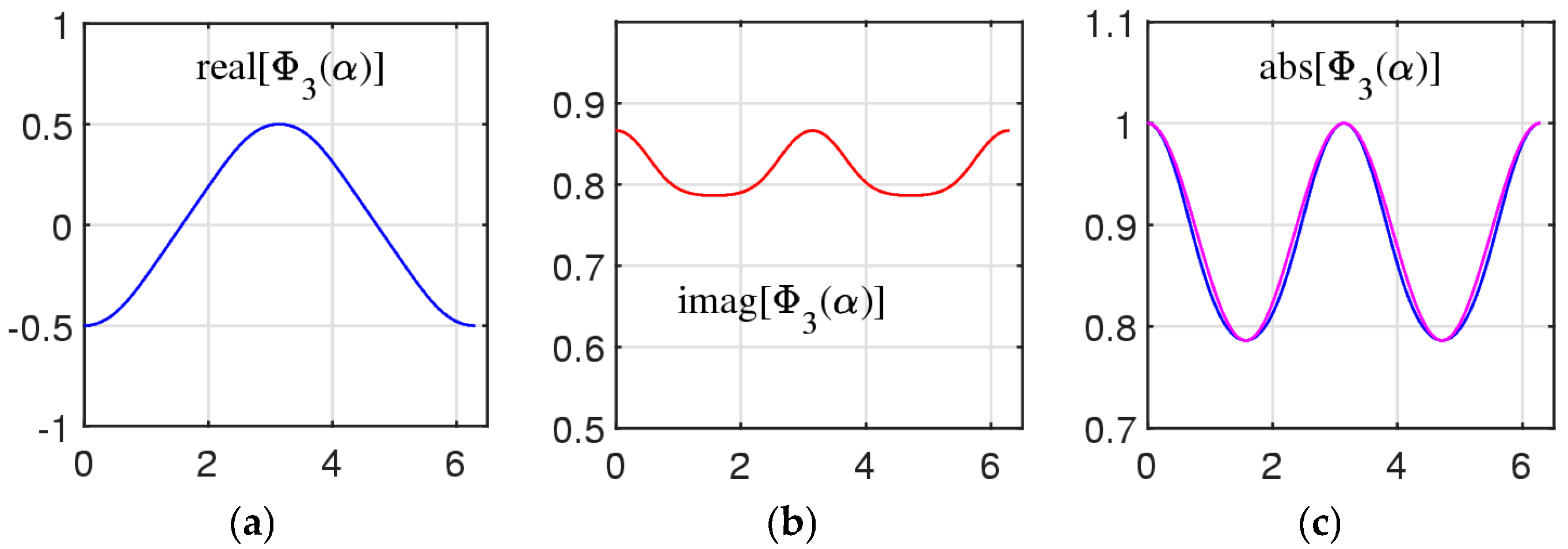
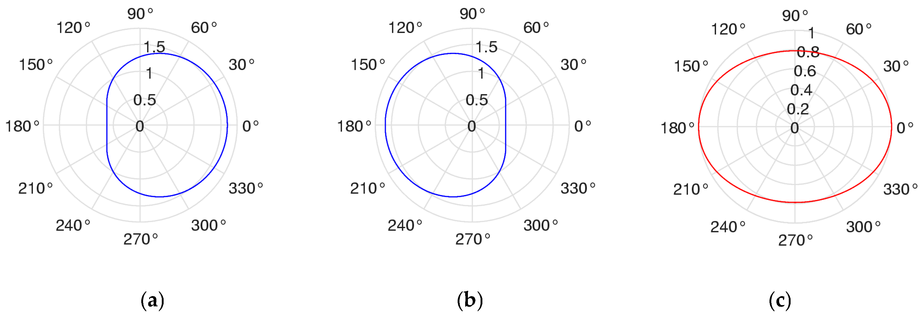
3.2. Analyze of Solutions

It is not difficult to note from Figure 9 that, for each angle, there are two real solutions of Equation (9). Even more, there is only one positive solution for each angle (see also Figure 7c). We will regroup the obtained set of roots x 1 ( α ) , x 2 α ,   x 3 α , and x 4 ( α ) of the above equation in the following way. The corresponding codes for these four roots are given in Appendix A.
For each angle α [ 0,2 π ] , the first two roots are real and the next two roots are a complex conjugate. Then, the real solutions are composed as follows:
Φ 1 α = x 1 α ,     i f   x 1 α 0 ; x 2 α ,    i f   x 2 α 0 ,        Φ 2 α = x 2 α ,    i f    x 1 α 0 ; x 1 α ,     i f    x 2 α 0 .
Figure 12 shows these two roots (solutions) in part (a) . The functions Φ 1 α and Φ 2 α are continuous. The first function is positive and the second one is negative. Both functions are periodic; the period is 2 π . It is interesting to note that Φ 1 α + π = Φ 2 α ,   α 0 , π .   In part (b), the graph of the sum of these solutions is shown: Ψ α = Φ 1 α + Φ 2 α . The magnitude of this function | Ψ α | 1 . The product of these functions with values in the interval [ 1.618033 , 1 ] is shown in part (c).
It is interesting to note that the graph of Ψ α in Figure 12b is similar to, but not exactly, the cosine function. This sum of two roots together with the cosine function cos ( α ) are shown in Figure 13a. The difference of these functions is given in part (b). The maximum difference of these two functions is 0.0344590758 (the functions were calculated for N = 2 20 + 1 angles α in the interval [ 0,2 π ] ) . Thus, the sum Φ 1 α + Φ 2 α can be considered as an approximation of the cosine wave cos ( α ) .
Figure 14 shows the graph of the positive roots Φ 1 α calculated in the interval [ 0,2 π ] . We call the function Φ ( α ) = Φ 1 α with this graph the general golden ratio function, or the GGR function. For this function, the minimum is 0.6180 at the angle point π , and the maximum is 1.6180 at 0 and 2 π . The golden ratio function is equal to 1 at angles of 2 / 3 π and 4 / 3 π . The mean of the golden ratio in this interval equals 1.192880 approximately at angles of 1.7385 and 4.5447 in radians, or 99.6075 ° and 260.3925 °   ( o r   180 ° 80.3925 ° ) .
The GGR function Φ ( α ) has a shape roughly similar to the cosine function. Together with the GGR function, the following function is shown in Figure 15:
y α = 1 2 Φ 1 ( 0 ) + Φ 1 ( π ) + cos α = 1 2 1.6180 + 0.6180 + 1 2 cos α = 1.1180 + 1 2 cos α .    
Figure 16 shows the graph of the GGR function versus angles in degrees in the interval [ 0 ° , 360 ° ] . A few points on the graph are marked for the values of this function at angles of 36 ° ,   72 ° ,   108 ° , and 144 ° , plus the angle 290.70 ° , at which the golden ratio is equal to 2 .
The complex roots of Equation (9) can also be regrouped by using the phases of complex solutions x 3 α = x 3 α e i ϑ 3 α and x 4 α = x 4 α e i ϑ 4 α . Namely the following functions are calculated:
Φ 3 α = x 3 α ,    i f    ϑ 3 α 0 ; x 4 α ,     i f     ϑ 4 α > 0 ,        Φ 4 α = x 4 α ,     i f     ϑ 3 α 0 ; x 3 α ,     i f   ϑ 4 α > 0 .
Note that   ϑ 4 α = ϑ 3 α . MATLAB-based codes for these functions are given in Appendix A.
Figure 17 shows the graphs of the real and imaginary parts of the complex solution Φ 3 α in parts (a) and (b), respectively. It can be noted that the real part of the solution Φ 3 α has values in the interval 0.5,0.5 . The absolute value of this function together with the function F α = Δ Φ 3 × ( cos 2 α 1 ) / 2   + 1 is shown in part (c). Here, Δ Φ 3 = max | Φ 3 α | min | Φ 3 α | = 0.213849 . The function F α can be considered as an approximation of | Φ 3 α | .
Figure 18 shows the magnitudes of three solutions, Φ k α , k = 1 : 3 , in the polar form. In comparison with the plots in Figure 10, one can note the symmetry of the plots of the real functions Φ 1 α and Φ 2 α . The polar plots for two other complex functions, Φ 3 α and Φ 4 α , are the same; the functions are complex conjugates to each other.

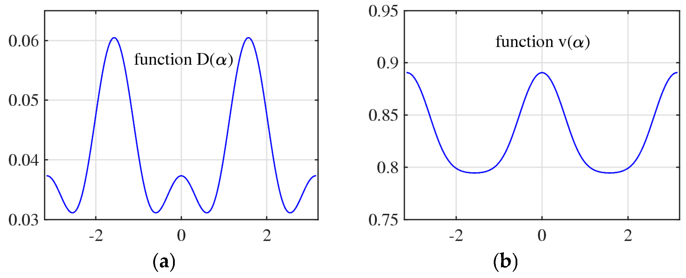
3.3. Properties of the Roots

The following properties are true for the roots of the golden equation:
Φ k α = Φ k α    a n d    Φ k α + 2 π = Φ k α ,   k = 1 : 4 ,  
Φ 1 α > 0    a n d    Φ 2 α < 0 ,     f o r   a l l   α ,
Φ 3 α , Φ 4 α C a n d Φ 3 α = Φ 4 ¯ α ,  
The coefficients of Equation (9) are 1,0 , 1 , 2 cos ( α ) , and 1 . Therefore, the Vieta’s formulas for this equation can be written as
Φ 1 α + Φ 2 α + Φ 3 α + Φ 4 α = 0
Φ 1 α Φ 2 α Φ 3 α Φ 4 α = 1 ,    
i j k 4 Φ i α Φ j α Φ k α = 2 cos ( α ) .  
i j 4 Φ i α Φ j α = 1 ,   
Due to Equations (23) and (24), the real part R ( Φ 3 α ) of the third solution (shown in Figure 17) is equal to [ Φ 1 α + Φ 2 α ] / 2 (see Figure 12b). It is also not difficult to see that these solutions are transformed into each other under the transformation α α + π . Indeed, the following identities are valid, for any angle α :
Φ 1 α = Φ 2 α + π ,     Φ 3 α = Φ 4 α + π .  
Thus, for each angle α , the real ratios can be in two states as φ α = Φ 1 α , Φ 2 α . This vector state changes with the operator α α + π as φ α + π = Φ 2 α , Φ 1 α . The full 4D vector of states changes as
Φ 1 α , Φ 2 α , Φ 3 α , Φ 4 α α α + π Φ 2 α , Φ 1 α , Φ 4 α , Φ 3 α .

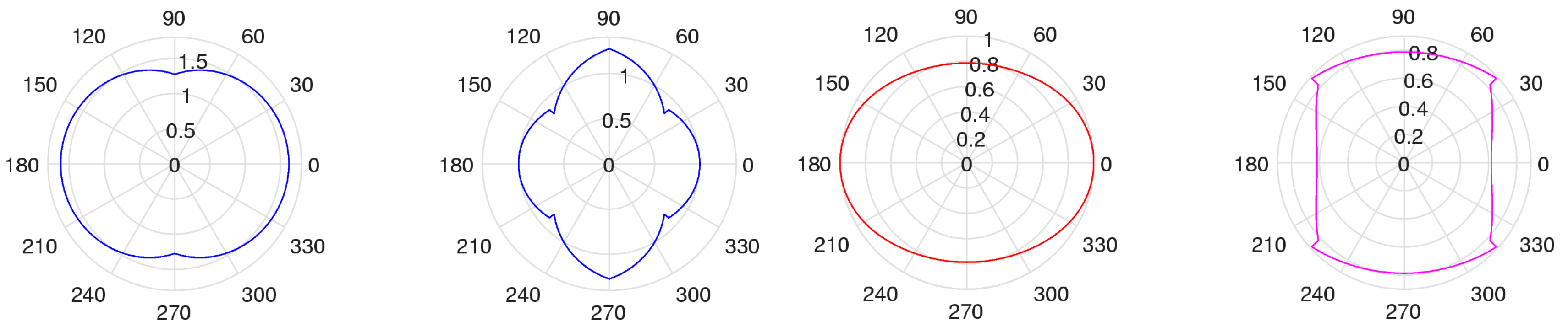
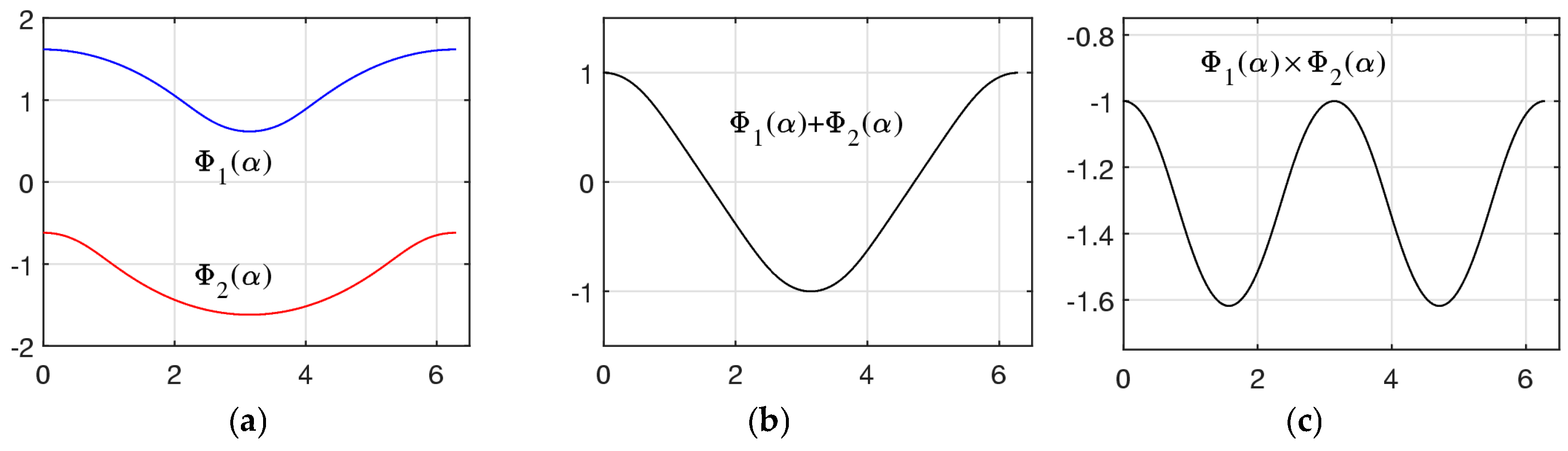
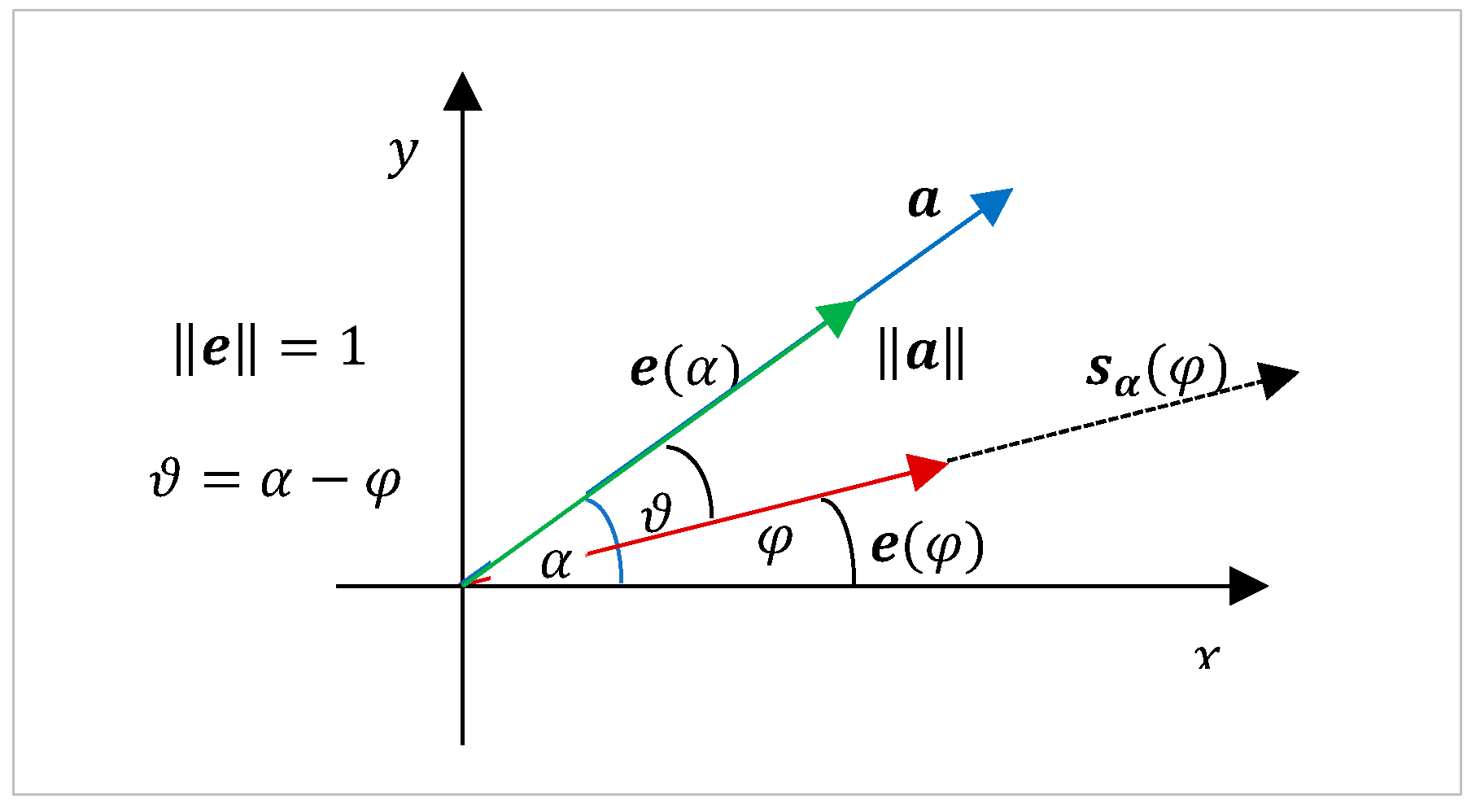
4. The Set of Similarity of a Vector

In this section, we consider a few examples of golden pairs of vectors in 1D and 2D vector spaces. The concept of the similarity set of the vector is also presented.
Example 3
(1D vectors). For 1D vectors (real numbers), or the elements of the real line R , we define the inner product as  a , b = a b . Then, the angle is defined as
cos α = a b a b = a b a | b | = s i g n a b ,
which means that the angle between similar elements may take only two values, 0 and π. Therefore, the set of similarity, that is, the set of numbers that are in the golden ratios with the number   a ,   is defined as
S a = a = a Φ arccos s i g n a b s i g n b ; b = ± 1 .  
When a > 0 , that is, s i g n a = 1 , the number a is in the golden ratio with the numbers of the set
S a = a Φ 0 , a Φ π .
When a < 0 , that is, s i g n a = 1 , the golden pairs are defined by the similarity set
S a = a Φ π , a Φ 0 .
These two sets are equal up to the sign. Here,
Φ 0 = 1 + 5 2 = 1.6180339887 , Φ ( π ) = 1 + 5 2 = 0.6180339887 .
Note that Φ 0 Φ π = 1 and Φ 0 Φ π = 1 . Thus, for number a >0, the set of similarities is equal to
S a = a = a Φ 0 , a Φ π = a Φ 0 , Φ π = a Φ 0 , 1 Φ 0 .
For the unit vector a = e = 1 , the set of similarity is S e = e = Φ 0 , 1 Φ 0 . The golden pairs are { 1 , Φ 0 } and 1,1 Φ 0 .
Example 4
(2D vectors). Consider two vectors a = [ a 1 , a 2 ] and b = [ b 1 , b 2 ] in the 2D real space R 2 . The inner product is defined as a , b = a 1 b 1 + a 2 b 2 and the norm of the vector a is equal to  a = a 1 2 + a 2 2 . All unit vectors e have tips on the unit circle; that is, they are described by the set
e e φ = ( cos φ , sin φ ) ;   φ [ 0,2 π ) .
We consider the polar form of the vector  a = a cos α , sin α , α 0,2 π   and a unit vector  e = e φ  at an angle  φ  to the horizontal (see Figure 19).
Let us assume that the unit vector e φ composes the angle ϑ with the vector a . The inner product of e φ with the unit vector e α = a / a along the vector a is equal to
e α , e φ = cos α cos φ + sin α sin φ = cos ( α φ ) = cos ϑ .
Definition 4.
Along the angle φ [ 0,2 π ) , the vector that is in the golden ratio with the vector a is equal to
s a φ = a Φ ϑ e φ = a Φ α φ e φ .  
An illustration of the golden pair of vectors { a , s a φ } is given in  Figure 19. The length of the vector  s a φ  is defined by the value of the GGR function at the angle of  ϑ = α φ ; that is, the angle between the vectors  a  and  e φ  , or s a φ . Therefore, the set of similarity of the vector  a  is defined as
S a = { s a φ ;   φ [ 0,2 π ) } = a Φ α φ e φ ;   φ [ 0,2 π ) .  
Thus, for a given vector  a , a golden pair can be found along any direction. The golden ratio changes with angles. As an example,  Figure 20 shows the locus of all similarity 2D vectors  s a φ  that compose the golden pairs  a , s a φ ,  for the vectors  a = [ 1,2 ]  and  [ 1,3 ]  in parts (a) and (b), respectively. The similarity sets of these vectors are
S 1,2 = s 1,2 φ ;   φ [ 0,2 π ) = 5 Φ tan 1 2 φ e φ ;   φ [ 0,2 π )
and
S 1,3 = s 1,3 φ ;   φ [ 0,2 π ) = 10 Φ π tan 1 3 φ e φ ;   φ [ 0,2 π ) .
In these figures, the vectors are shown only for 128 uniformly distributed angles  φ  in the interval [ 0,2 π ) . The figures recall the same petal rotated by different angles and magnifications. Each vector  a  shows the orientation of the corresponding set of similarity  S a .
Figure 20. The locus of 128 golden pairs with the vectors (a) a = [ 1,2 ] and (b) a = 1,3 . (c) The locus of 128 golden pairs with the unit vector e = 1,0 .
Mathematics 13 00699 g020
In part (c), the similarity figure is shown for the vector a = e = 1,0 . The similarity set of this unit vector is
S 1,0 = s 1,0 φ ;   φ [ 0,2 π ) = Φ φ e φ ;   φ [ 0,2 π ) = Φ φ e φ ;   φ [ 0,2 π ) .
It should be noted that the figures of the sets of similarity in part (a) and (b) are the rotated figure of part (c) with magnification by the norms 5 and 10 of the vectors a = [ 1,2 ] and 1,3 , respectively. The figure of the set S 1,2 can be obtained from the figure of the set S 1,0 by rotating it by the angle of tan 1 2 and increasing it by 5 times. Similarly, the figure of the similar set S 1,2 in part (b) can be obtained from the figure of S 1,0 by rotating it by the angle of ( π tan 1 3 ) and increasing it by 10 times.

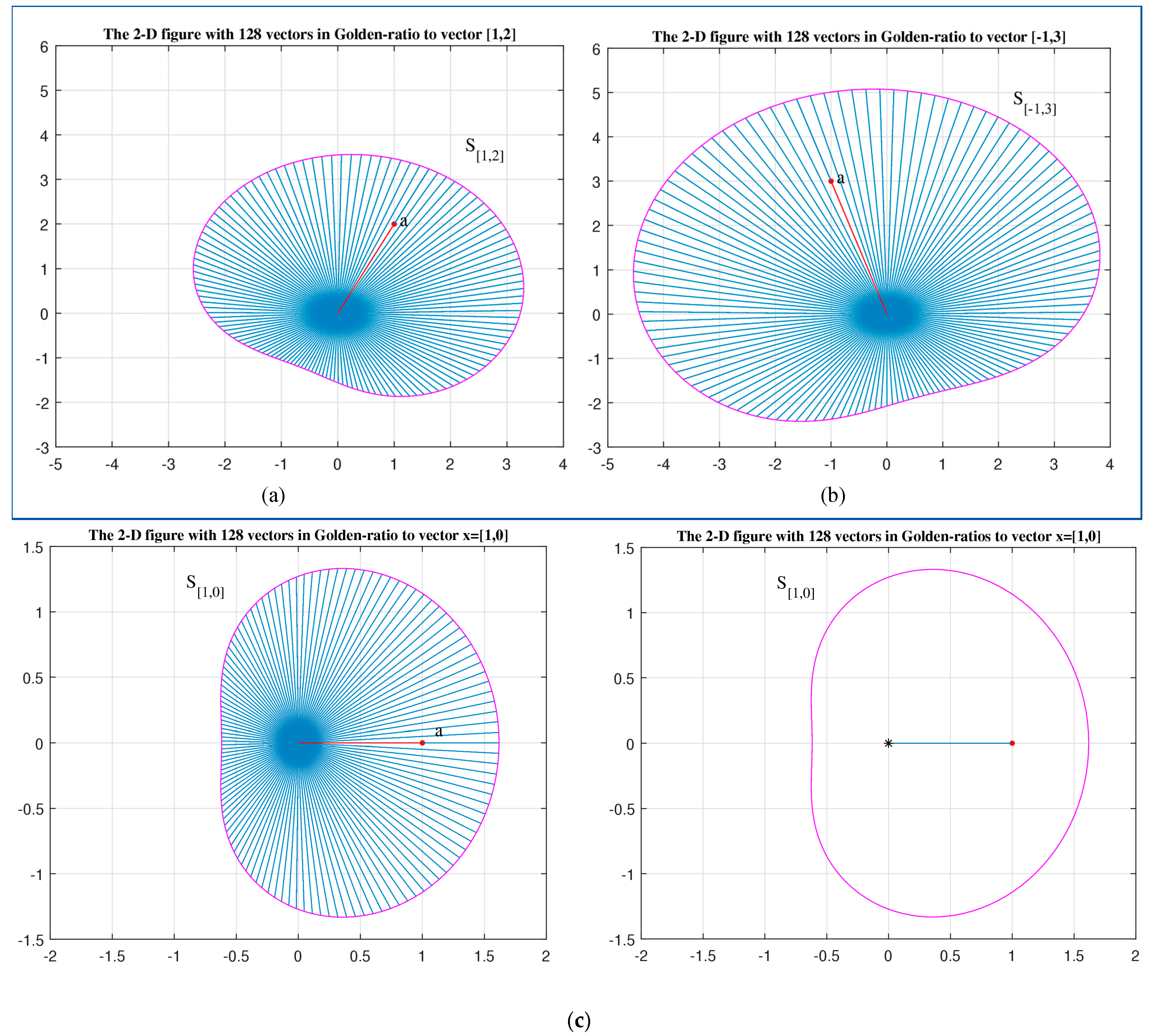
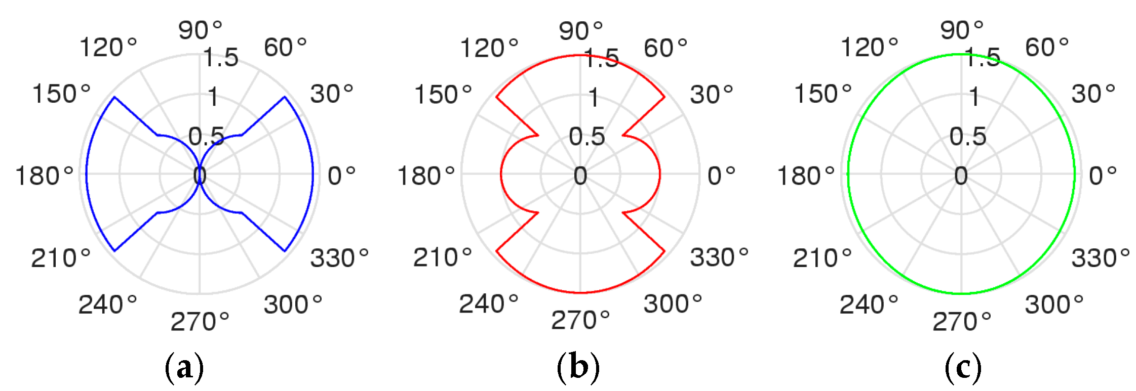
5. Field of Similarities

A. Philosophical digression: What is similarity in our case? Each vector affects its environment by stimulating its influence through the imposition of its likeness. The vector may represent a force, an impulse, or any action in the vector space. If you think about it, this means we are all a certain vector of possibilities that we impose on the environment by projecting ourselves into it, and this projection is symbolically represented by a certain projection angle.
The vector or force in its action can be expressed (presented) by one of its similarity vectors (or forces) in any direction. All these possible similarities, or states of vectors, do not describe the ideal unit circle in a 2D plane for one qubit or the unit sphere in a 3D space for two qubits, as assumed in the quantum computing [20]. Here, we have the figure of a petal in the 2D case (Figure 20) and an apple in the 3D case (as shown in the next section).
B. So far we have known that if two vectors do not interact and their inner product is zero (that is, the angle between the vectors is 90 degrees), then mutual influence is excluded. But what is interesting is that the similarity coefficient at this angle is not equal to zero! That is, the influence is still there. According to the printout, it appears that
Φ π 2 = Φ 0 = 1 + 5 2 = 1.2720196495
C. Two roots of Equation (9) are real, Φ 1 α and Φ 2 α . The second one is negative. Note that negative numbers do not exist in nature. We can talk about two, three, etc. objects, which we can not only imagine, but also see (let us s say, 2, 2.5, and 3 apples). One cannot say that about negative numbers; only the imagination works here (let us imagine 3 apples). We can say that positive or negative number are two states, like heads and tails in the probability theory. After all, it was not for nothing that we found two states, φ α = Φ 1 α , Φ 2 α ; one refers to positive roots, and the other to negative ones. Two other solutions are complex, Φ 3 α and Φ 4 α ; they show us the 2D representation ψ α = Φ 3 α , Φ 4 α (the real solutions determine the 1D representation).
D. (The sum of similarity vectors) The following question arises: is it possible to add similarity fields? If so, then what exactly does the sum of similarities mean? Let us consider two different vectors, a 1 and a 2 , at angles of α 1 = arg ( a 1 ) and α 2 = arg ( a 2 ) to the positive real axis, respectively. The corresponding sets of similarities are
S a 1 = s a 1 φ ;   φ [ 0,2 π ) = a 1 Φ α 1 φ e φ ;   φ [ 0,2 π ) ,   
S a 2 = { s a 2 φ ;   φ [ 0,2 π ) } = a 2 Φ α 2 φ e φ ;   φ [ 0,2 π ) .  
These two sets can be written as
S a 1 = a 1 Φ φ e α 1 φ ; φ [ 0,2 π )
S a 2 = a 2 Φ φ e α 2 φ ; φ [ 0,2 π ) .
Definition 5.
The sum of the sets of similarities is the set of similarities
S a 1 + a 2 = a 1 + a 2 Φ γ φ e φ ;   φ [ 0,2 π ) ,   
where the angle  γ = arg a 1 + a 2 .  
Let us verify if the following is true:
S a 1 + a 2 = S a 1 + S a 2 .    
Here, the summation is angle-wise; that is, the summation of vectors that correspond to the same angle φ . Therefore, this equation can be written as
a 1 + a 2 Φ φ e γ φ = a 1 Φ φ e α 1 φ + a 2 Φ φ e α 2 φ .
All vectors have the same coefficient of similarity. Removing the similar term Φ φ from this equation, we obtain
a 1 + a 2 e γ φ = a 1 e α 1 φ + a 2 e α 2 φ .
This equation describes the well-known rule for summing vectors over projections. The following calculations are valid for the right part of this equation:
a 1 e α 1 φ + a 2 e α 2 φ = a 1 cos ( α 1 φ ) , sin ( α 1 φ ) + a 2 cos ( α 2 φ ) , sin ( α 2 φ ) = a 1 cos ( α 1 ) cos ( φ ) + sin ( α 1 ) sin ( φ ) , sin ( α 1 ) cos ( φ ) cos ( α 1 ) sin ( φ ) + a 2 cos ( α 2 ) cos ( φ ) + sin ( α 2 ) sin ( φ ) , sin ( α 2 ) cos ( φ ) cos ( α 2 ) sin ( φ ) = ( a 1 ) x cos ( φ ) + ( a 1 ) y sin ( φ ) , ( a 1 ) y cos ( φ ) ( a 1 ) x sin ( φ ) + ( a 2 ) x cos ( φ ) + ( a 2 ) y sin ( φ ) , ( a 2 ) y cos ( φ ) ( a 2 ) x sin ( φ ) = [ ( a 1 ) x + ( a 2 ) x cos ( φ ) + ( a 1 ) y + ( a 2 ) y sin ( φ ) , ( a 1 ) y + ( a 2 ) y cos ( φ ) ( a 1 ) x + ( a 2 ) x sin ( φ ) ] = ( a 1 + a 2 ) x cos ( φ ) + ( a 1 + a 2 ) y sin ( φ ) , ( a 1 + a 2 ) y cos ( φ ) ( a 1 + a 2 ) x sin ( φ ) = a 1 + a 2 cos ( γ φ ) , sin ( γ φ ) = a 1 + a 2 e γ φ .
Here, ( a 1 ) x = a 1 cos ( α 1 ) ,   ( a 1 ) y = a 1 sin ( α 1 ) ,   ( a 2 ) x = a 2 cos ( α 2 ) ,   ( a 2 ) y = a 2 sin ( α 2 ) , and ( a 1 + a 2 ) x = a 1 + a 2 cos ( γ ) , and ( a 1 + a 2 ) y = a 1 + a 2 sin ( γ ) . Thus, everything is correct in Equations (38) and (39).
Figure 21 illustrates this property in part (b), where the parallelogram is the result of the rotation of the original parallelogram in part (a), which is composed by the vectors a 1 and a 2 .
As examples, Figure 22 illustrates the summation of the similarity sets for the vectors a 1 = [ 1,2 ] and a 2 = [ 1,3 ] in part (a) and for the vectors a 1 = [ 2 , 3 ] and a 2 = [ 1,5 ] in part (b).
Figure 23 shows the same sum S [ 1,1 ] of similarity sets for three pairs of vectors a 1 and a 2 , namely for the vectors [ 0,1 ] and 1,0 in part (a), the vectors [ 1,2 ] and 0 , 1 in part (b), and the vectors [ 2,3 ] and 1 , 2 in part (c). If we assume that the vectors represent forces and generate the similarity fields, then the above figures with the sums of similarity sets (fields) illustrate the influence of fields on a space; for example, attraction and repulsion.
It should be noted that we do not sum the similarity sets over equally directed rays. If we were to perform this, that is, if we consider the sum of the similar vectors
A = a 1 Φ α 1 φ e φ + a 2 Φ α 2 φ e φ
for each angle φ 0,2 π , then we need to find the vector a 0 and angle γ 0 such that a 0 Φ γ 0 φ e φ = A .   The solution of the equation
a 0 Φ γ 0 φ = a 1 Φ α 1 φ + a 2 Φ α 2 φ ,    φ [ 0,2 π ) ,
is unknown for us.
Example 5
(3D vectors). We consider the traditional representation of the 3D unit vectors, namely the set
e = sin φ cos ψ , sin φ sin ψ , cos φ ;   φ 0 , π ,   ψ [ 0,2 π ) .
The geometry of the unit vector  e = e φ , ψ = sin φ cos ψ , sin φ sin ψ , cos φ  is shown in Figure 24.
The inner product of this unit vector e with a vector a = a sin φ 1 cos ψ 1 , sin φ 1 sin ψ 1 , cos φ 1 , where φ 1 0 , π ,   ψ 1 [ 0,2 π ) , is calculated by
e , a = a cos ϑ = a sin φ cos ψ sin φ 1 cos ψ 1 + sin φ sin ψ sin φ 1 sin ψ 1 + cos φ cos φ 1 .
Thus,
cos ϑ = sin φ cos ψ sin φ 1 cos ψ 1 + sin φ sin ψ sin φ 1 sin ψ 1 + cos φ cos φ 1 .
The cosine of the angle between these two vectors is the function of four arguments; that is, the angle ϑ between the vectors e and a is the function ϑ = ϑ ( φ , ψ ,   φ 1 , ψ 1 ) .
Definition 6.
The similarity set, that is, the set of all vectors in the golden ratio with the vector  a ,  is
S a = a Φ ϑ sin φ cos ψ , sin φ sin ψ , cos φ ;   φ 0 , π ,   ψ 0,2 π .   
Let a be the unit vector e 3 = 0,0 , 1 .  Figure 25 shows the locus of vectors being in the golden ratio with this vector in part (a). In this case, φ 1 = 0   and cos ϑ = cos ϑ ( φ , ψ ,   0 , ψ 1 ) = cos φ . Therefore, ϑ = φ and the set of similarity is
S e 3 = Φ φ sin φ cos ψ , sin φ sin ψ , cos φ ;   φ 0 , π ,   ψ 0,2 π .  
We also consider the unit vector a = e 1 = 1,0 , 0 . Then, φ 1 = π / 2 ,   ψ 1 = 0 , and cos ϑ = cos ϑ ( φ , ψ ,   π / 2,0 ) = sin φ cos ψ . Therefore, ϑ = arccos ( sin φ cos ψ ) and the similar set is
S e 1 = Φ ϑ sin φ cos ψ , sin φ sin ψ , cos φ ;   φ 0 , π ,   ψ 0,2 π .   
The locus of vectors of this similarity set is shown in part (b). In these two figures, as in the 2D case above, only the ends of the vectors as dots are shown. The angles φ and ψ were taken with the step 2 π / 512 in the intervals 0 , π and 0,2 π , respectively. Figure 26 and Figure 27 show these similar sets by different angles, namely by using the azimuth (AZ) of zero degree and vertical elevation (EL) of 90 and 180 degrees, respectively. For this, the MATLAB functions ‘view(2)’ and ‘view(0,180)’ were used.
Figure 28 shows the 3D surface that is made up of the vertices of the vectors of a subset of S e 3 in part (a). This is the surface that frames the vectors which are similar to the unit vector e 3 = 0,0 , 1 . In part (b), the similarity surface is shown for the unit vector e 1 = 1,0 , 0 . For both surfaces, the angles φ and ψ were taken with the step 2 π / 360 in the intervals 0 , π and 0,2 π , respectively.

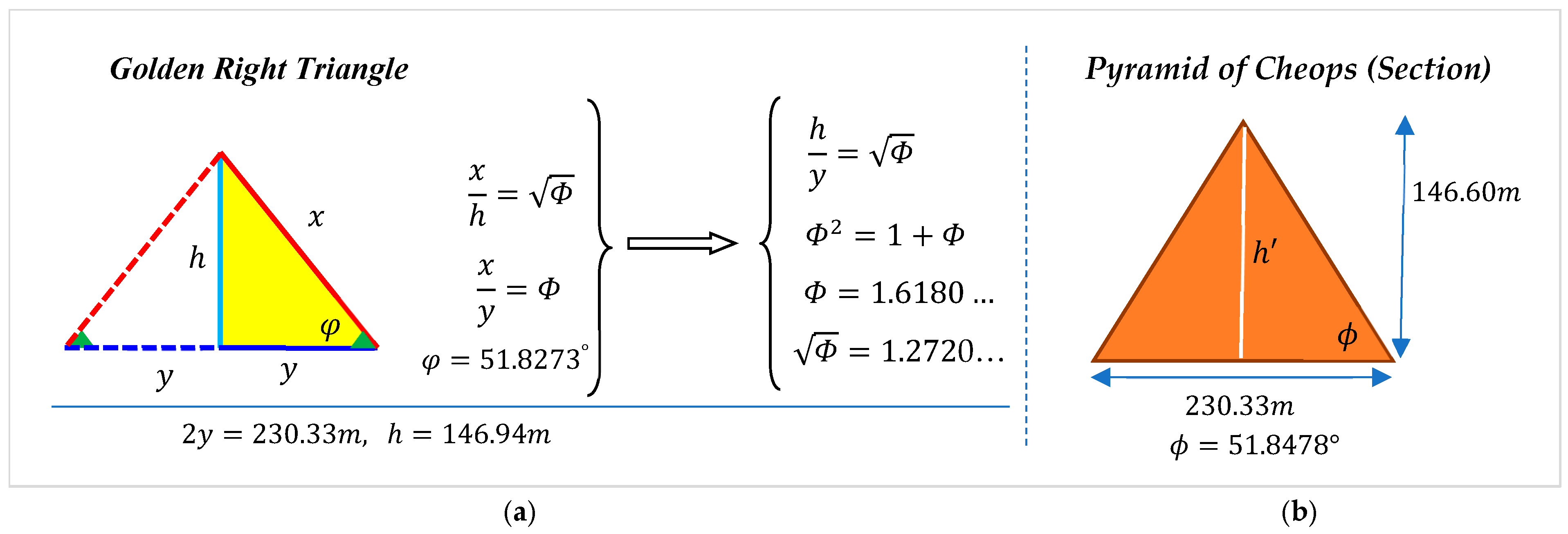
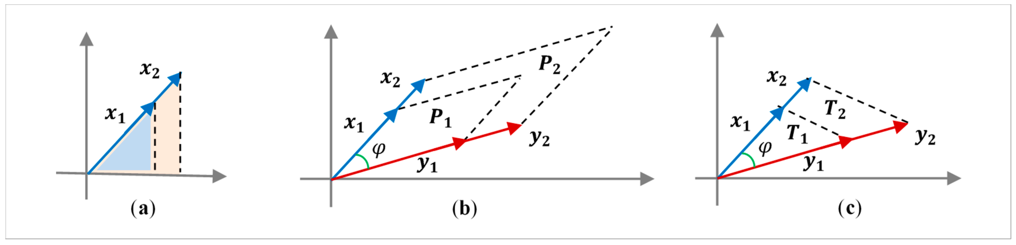
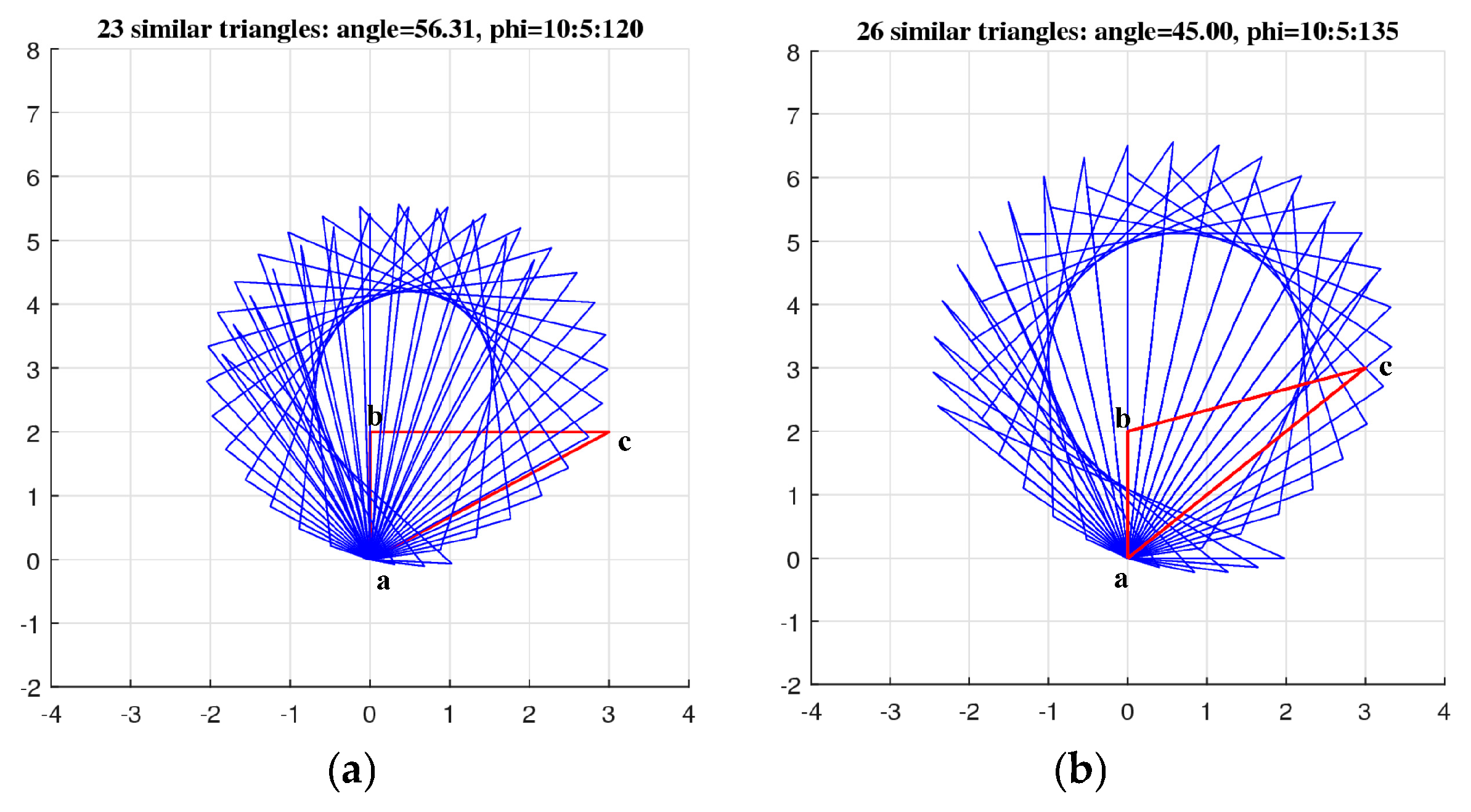
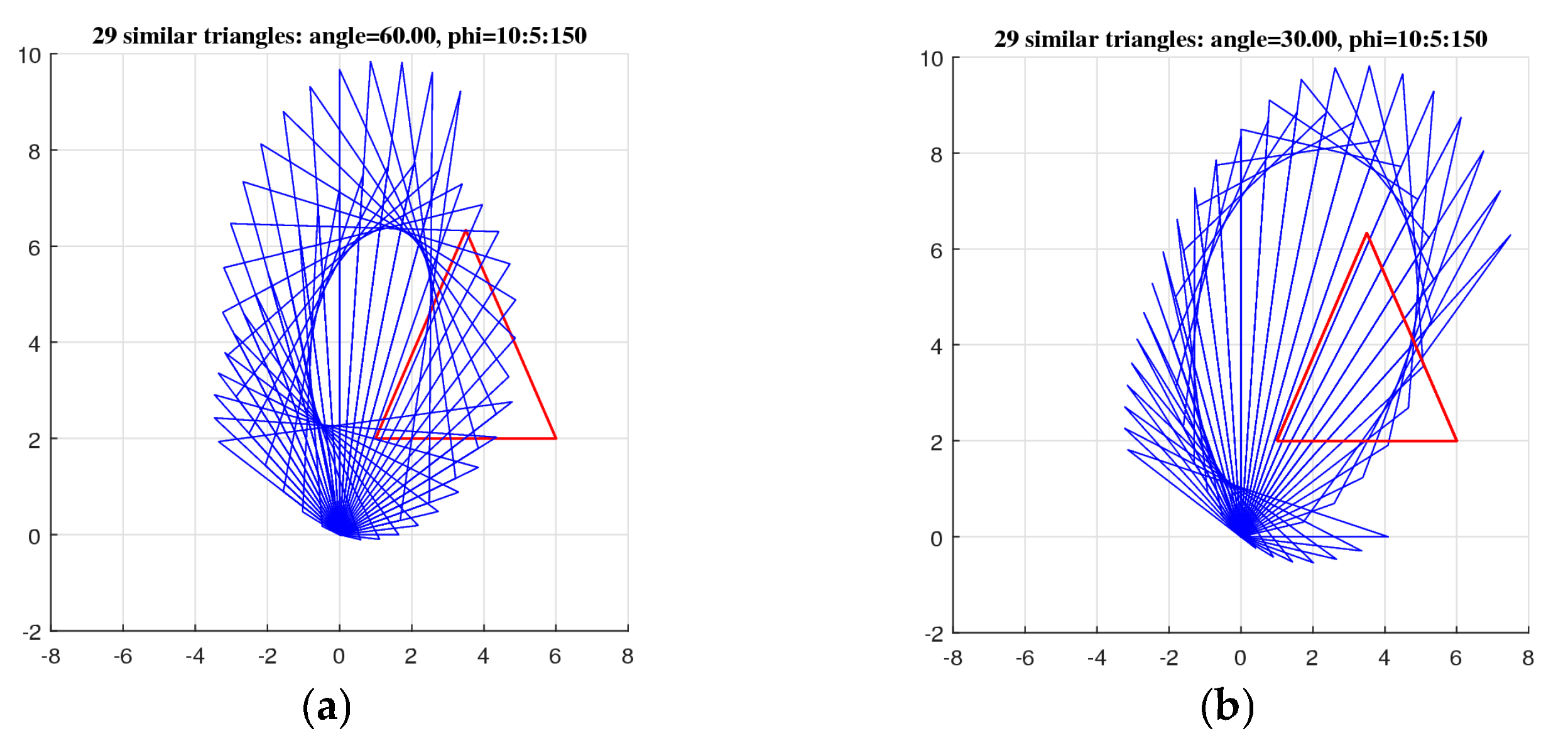
6. Similarity Triangles in Golden Ratio

In this section, we consider triangles as elements of a 6D vector space and introduce the concept of the inner product and norm of triangles. The triangles in the golden ratio are described, and the similarity sets of triangles are presented with examples. Other polygons can be described in a multidimensional space in a similar way.
In order to show the similarity of three points ( a , b , c ) in the form of a triangle on the plane (see Figure 29a), we need three 2D vectors, which we denote by v a , v b , and v c . The vectors being v a = x a , y a ,   v b = x b , y b , and v c = x c , y c . These coordinate vectors compose the 6D vector V = v a , v b , v c . Consider two 6D vectors that correspond to two triangles, V 1 = v a 1 , v b 1 , v c 1 and V 2 = v a 2 , v b 2 , v c 2 . The inner product of these vectors is defined as
V 1 , V 2 = v a 1 v b 1 , v a 2 v b 2 + v b 1 v c 1 , v b 2 v c 2 + v c 1 v a 1 , v c 2 v a 2 .  
The norm of the vector is defined as
V 2 = V , V = v a v b 2 + v b v c 2 + v c v a 2 .  
The norm V = 0 ,   when a triangle degenerates into a point, that is, when v a = v b = v c , and this case is not considered. The case where a triangle turns into a straight line is also not considered.
A unit vector, or a triangle, E = e a , e b , e c with norm 1 is defined as
E 2 = e a e b 2 + e b e c 2 + e c e a 2 = 1 .  
We can zero the first 2D vector e a   and consider the unit vector E = 0 , e b , e c , for which
E 2 = e b 2 + e b e c 2 + e c 2 = 1 ,   
provided that e b e c ,   e b 0 , and e c 0 . This 6D vector corresponds to a triangle with the point a at the center of the system of coordinates. An example of such a triangle is shown in Figure 29b.
It follows from Equation (48) that
2 e b 2 2 e b e c cos ( λ ) + 2 e c 2 = 1
Here, λ is the angle between 2D vectors e b and e c . This equation can be written as
e b 1 2 e c cos ( λ ) 2 + 1 4 e c 2 4 cos 2 ( λ ) = 1 2 .  
Solutions of this equation can be written as ( λ 0 ) :
e b 1 2 e c cos ( λ ) = 1 2 cos ϕ , 1 2 e c 4 cos 2 ( λ ) = 1 2 sin ϕ ,
where ϕ 0 , π λ . Thus, we have a parameterized set of solutions; two parameters are the angles λ and ϕ . The solutions can be written as
e c = 2 / 4 cos 2 ( λ ) sin ϕ , e b = 1 2 e c cos ( λ ) + 1 2 cos ϕ .  
Here, 0 < ϕ π λ and 0 < λ < π . This system of solutions connects the lengths and the angle λ between the sides of the triangle, e b and e c . Note that, to generalize this solution, we can add a zero element V c = c , c , c with norm 0. Indeed, for the 2D vector c = c 1 , c 2 0,0 ,   E + V c = E =1.
The vector E = e a , e b , e c can be analytically written as
Mathematics 13 00699 i001
The angles ϕ in Equations (51) and (52) are considered the same.
Thus, the vector is parameterized by two angles; that is, E = E ϕ , λ . In this system, the vector e c is rotated counter clock-wise by the angle ϕ and the vector e a   by the angle ( λ + ϕ ) (from the horizontal). We denote the set of such unit 6D vectors (triangles) E by E . As examples, Figure 30 shows five unit triangles with the angle λ = 40 ° . The first triangle with angle ϕ = 10 o is shown in red with the vertices marked. The other four unit triangles are shown for the angles ϕ = 40 ° , 70 ° , 100 ° , and 130 ° .
Two other examples with unit triangles are shown in Figure 31. Four unit triangles with angle λ = 60 ° are shown in part (a), when angles ϕ = 10 ° , 40 ° , 70 ° , and 100 ° . In part (b), three unit triangles with angle λ = 110 ° are shown, when ϕ = 10 ° , 40 ° , and 70 ° .
For a triangle described by a 6D vector V = v a , v b , v c , the similarity triangle, or the triangle in the general golden ratio with V , is defined as
s V ϕ , λ = V Φ ϑ E ϕ , λ ,     λ 0 , π ,    0 < ϕ π λ
Here, ϑ = a n g l e ( V , E ) denotes the angle between the vectors V and E = e a , e b , e c , which is calculated by
cos ϑ = V , E V .
The norm V is calculated as in Equation (47), and the inner product is calculated by
V , E = v a v b , e a e b + v b v c , e b e c + v c v a , e c e a .   
As an example, Figure 32 shows the triangle described by the vector V = v a , v b , v c = ( 0,0 , 3,2 , 5,0 ) in part (a). The angle between the vectors v b and v c is equal to θ = 33.69 ° , and Φ ϑ = 1.5702 . The similarity triangles s V 20 ° , λ ,   s V 40 ° , λ , and s V 70 ° , λ , for angle λ = θ , are shown in parts (b), (c), and (d), respectively.
Statement 1.
For the vector  V = v a , v b , v c , the similarity set of triangles is defined as
S V = s V ϕ , λ ;   0 < ϕ π λ ,   0 < λ < π .
Also, we can write this set as  S V = V Φ ϑ E ;   E E ,   ϑ = a n g l e ( V , E ) .
As an example, Figure 33a shows the subset of the similarity set S V for the vector V = ( 0,0 , 0,2 , 3,2 ) , which represents a right triangle with an angle θ = 56.31 ° between sides ab and ac (shown in red). The angle θ = a n g l e ( v b , v c ) is the angle between the vectors v b and v c . The unit vectors E are calculated by Equations (51) and (52) for 23 angles ϕ = 10 ° : 5 ° : 120 ° . The second parameter λ = θ , that is, the angle between the vectors e b and e c in the similarity triangles, is the same as in the triangle for V . In part (b), the subset of another similarity set S V is shown for the vector V = ( 0,0 , 0,2 , 3,3 ) . This vector represents a triangle with the angle θ = 45 ° between vectors v b and v c (shown in red). Here, 26 angles of ϕ are used, namely ϕ = 10 ° : 5 ° : 135 ° and the angle λ = θ .
In Figure 34, the similarity subsets are shown for the equilateral triangle with sides having five units of length. The corresponding vector is V = ( 1,2 , 3.5,4 sin ( π / 3 ) , 7,2 ) . The first point a = [ 1,2 ] of the triangle is not at the origin. In part (a), the subset of similarity triangles is shown for 29 angles ϕ = 10 ° : 5 ° : 150 ° and angle λ = 60 ° . This is the case when λ = θ = 60 ° . In part (b), the subset is shown for the same 29 angles of ϕ and the angle λ = 30 ° .
As can be seen from the figures above, among similarity triangles, there are none equal to the triangle with the vector V . It also not difficult to see from Equation (53) that s V ϕ , λ = V only if
Φ ϑ E ϕ , λ = V V ,
that is, when Φ ϑ = 1 , or ϑ = 120 o and λ = ϑ . It is possible that other definitions of the inner product of triangles could lead to similarities that include the original triangle V .
As was mentioned above, to generalize this solution, we can add two unit vectors E = E ϕ , λ a zero element V c = c , c , c with a 2D vector c = c 1 , c 2 0,0 . Therefore, in general, we can consider the similarity set of triangles of the vector triangle V = v a , v b , v c as a set parameterized by angles ϕ , λ , and vector c :
S V = s V ϕ , λ , c ;   0 < ϕ π λ , 0 < λ < π ,   c R 2
To facilitate understanding, we can separate similarities by fixing two parameters out of three. Also, we can consider these similarities separately (as spatial similarity, similarity in one fixed angle λ , or similarity in rotation ϕ ). If we are interested in similarities with a fixed angle between two sides, then we should fix the value of λ, giving it the value of one of the angles of the original triangle. Adding a constant vector V c leads to a spatial shift (translation) of the set of similarities.

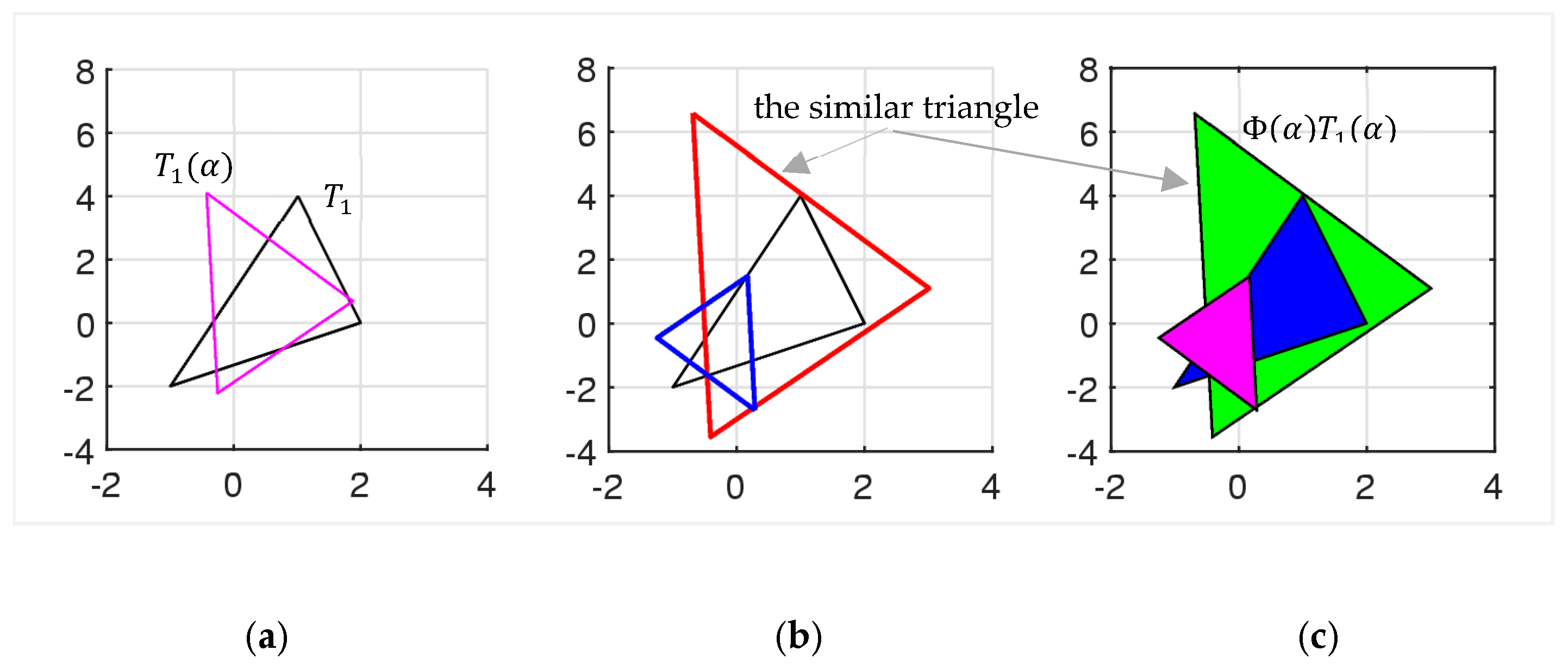
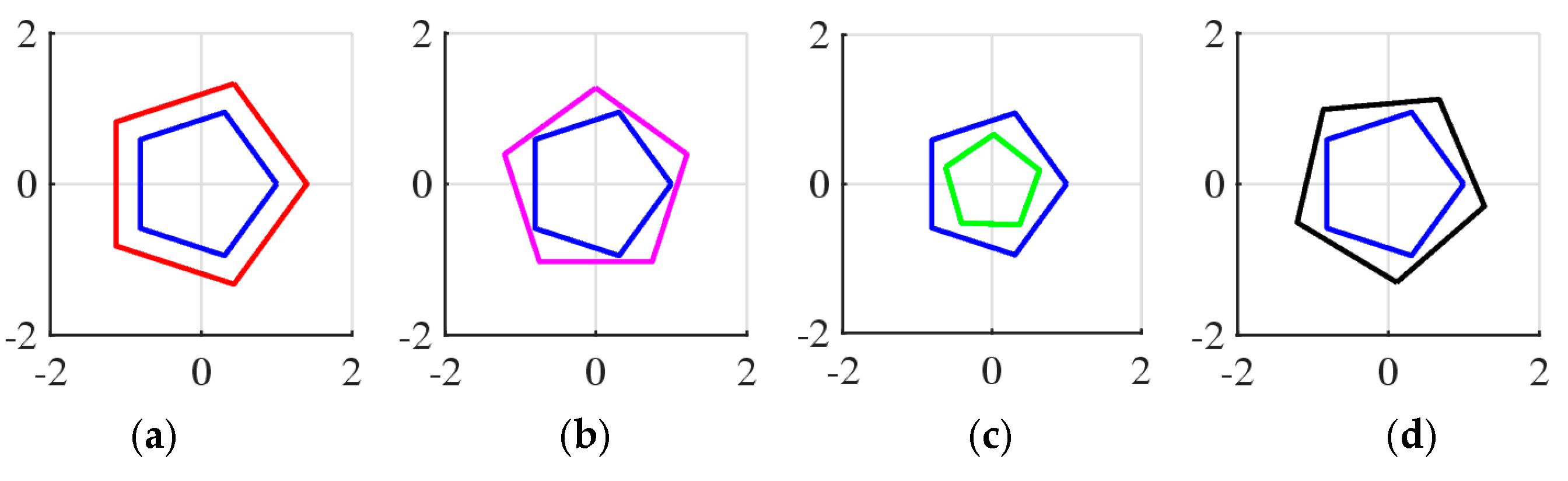
7. Similarity of Figures (Not Vectors)

The concepts of the similarity vectors and similarity sets of vectors, or golden vectors, are defined in the vector space. These concepts were described in detail and illustrated in Section 6 on examples with triangles represented as vectors. In this section, we present the concept of similarity on figures, without considering them as vectors. In general, it is difficult to describe many figures (objects), for example, the seven-pointed star, in the vector space. The generalized golden ratio function can also be used in the simple case for similar figures (or objects), considering the change in the size of a given figure according to this function, as the function of angle; that is, after rotating the figure. Now, we will illustrate this simplified concept of similar figures on examples in the 2D plane, which include well-known figures, such as pentagons, heptagons, stars, and spirals.
Example 6
(Triangle). Let us consider the following three points on the space: a = 1,4 ,   b = [ 1 , 2 ] , and c = 2,0 . These points together compose one triangle, which we denote by T 1 = { a , b , c } . We need to draw the triangles which are in the golden ratio with the triangle T 1 ( α ) rotated by α = 20 ° . Figure 35 shows the original triangle in part (a) (in black color) together with the rotated triangle (in magenta). The solutions of the golden equation for this angle are
{ x k α ; k = 1 : 4 } = { 1.6012 , 0.6632 , 0.4690 + 0.8496 i , 0.4690 0.8496 i }
Two roots are real, x 1 α = Φ α = 1.601185 .   and x 2 α = 0.66318359 , and only one is positive. The similar triangle, that is, the triangle in the golden ratio, T 2 = Φ ( α ) T 1 ( α ) is shown in part (b). The small triangle in part (b) is T 2 = x 4 ( α ) T 1 ( α ) , which is in the “negative” golden ratio with T 1 ( α ) . In part (c), the original triangle is shown in blue and the triangle in the gold ratio with it in green.
Note that the system of coordinates is not in the center of the triangle T 1 and the golden pair changes the original form (angles) of the triangle.

Other Figures

Now, we consider a few more illustrative examples for the GGR function in the 2D vector space. The figures of regular polygons and stars are considered with their centers at the initial point of the coordinate system. The shape of the golden pairs for each of these figures is preserved, as shown below.
Example 7.
Consider a pentagon, P 5 , inside the unit circle, which is shown in  Figure 36 in the blue color. The pentagons that are in the golden ratio with P 5  at angles of 72 ° , 90 ° , 160 ° , and 275 °  are shown in parts (a), (b), (c), and (d), respectively.
Example 8.
Consider a heptagon, P 7 , inside the unit circle, which is shown in  Figure 37 in the blue color. The heptagons that are in the golden ratio with P 7  at anglesof 30 ° , 140 ° , −100 ° , and 200 °  are shown in parts (a), (b), (c), and (d), respectively.
Example 9.
Consider a seven-pointed star, or the regular heptagram,  S 7,3 ,  inside the unit circle. This star is shown in  Figure 38 in the blue color. The heptagrams that are in the golden ratio with S 7,3  at anglesof30 ° , 90 ° , 160 ° , and 220 °  are shown in parts (a), (b), (c), and (d), respectively.
Example 10.
Consider a nine-pointed star, or the regular enneagram, S 9,4 ,  inside the unit circle. This star is shown in  Figure 39a. The enneagrams that are in the golden ratio with S 9,4  at angles of 90 ° , 160 ° , and 220 °  are shown in parts (b), (c), and (d), respectively.
Example 11.
Consider the figure with the cross, along with 10 half-size crosses, each of which is located in a circle, as shown in Figure 40a. This is a traditional picture with complete symmetry and identical figures. There is complete symmetry, and there is no movement in this picture. Part (b) shows the cross in the center together with its 10 crosses in the golden ratio at angles of 18 ° ,  54 ° ,   90 ° ,   126 ° , …, and 342 ° . The same cross in the center together with its 12 golden pairs at angles of 15 ° ,   45 ° ,   75 ° ,   105 ° ,  145 ° , …,  and 335 °  is shown in part (c).
Example 12.
Consider a 5-pointed star together with 12 stars of half of its size, which are shown in Figure 41. In part (a), the traditional picture is shown, and in part (b), 12 stars compose the golden pairs with the star in the center.
Example 13.
Consider the 7-pointed star, S 7,3 ,  shown in the center of  Figure 42 in part (a) and 12 golden pair stars placed around a circle. These golden pairs were calculated for a star half the size, S 7,3 / 2 . Figure 42a shows a similar picture for the nine-pointed star, S 9,4 . The golden pairs of these two stars were calculated for angles of 15 ° ,   45 ° ,   75 ° ,   105 ° ,145 ° , …,and 335 °  and are shown in parts (b) of these figures.
Example 14.
Consider the locus of the first 108 points on the Archimedes spiral  A 108 = { n e i n 180 / π ;   n = 108 } . We can call this figure a linear spiral A 108 . Figure 43 shows this spiral in the center together with eight spirals which compose the golden pairs with the spiral A 108 /2 of half the size. These eight spirals are placed around a circle at a distance of 45 ° .
If we superimpose these shapes on top of each other, we get a 3D shape. As examples, Figure 44 shows such a 2D view for the n -sided polygons P n for n = 4,5 , 6 ,   and 7. The angles α were taken from the interval [ 0,2 π ] with a step of 2 degrees. The original polygons P n are shown on the x-y plane in the black color.
Figure 45 shows such shapes for the square in part (a) and for the twelve-sided polygon (dodecagon) in part (b). In these shapes, the polygons in the golden ratios are colored randomly, and angles α were taken from the interval [ 0,2 π ] with the small step of 0.2 ° . These two figures exist in nature.

8. Afterword and Conclusions

In this work, we generalize the similarity law for multidimensional vectors. Initially, the law of similarity was derived for one-dimensional vectors. Although it operated with such values of the ratio of parts of the whole, this meant the use of linear dimensions (a line is one-dimensional). Now the question of where one can observe this generalization arises. If we refer to the forms of fruits, for instance, the apple, then it is easy to see a strongly pronounced broken sphericity, which does correspond to the listed forms.
The main part of this research is the concept of similarity, namely the set of similarity vectors to a given one. In all graphics above, the vectors were used, not the area or surface (in the 3D case). The vector represents the force. The full meaning of the concept of similarity is difficult to understand well or even grasp. There is a mystery here that we cannot solve. Intuitively, our subconscious mind shows that a certain vector spreads itself in the surrounding space. What we consider local, as a certain center of the outflow of a narrowly directing force, is an abstraction. Any force retains its likeness around itself and has spatial dimensions even in the opposite direction. Physically, it is hard to imagine. Psychologically, it can be imagined in the following way. If you accompany the realization of force, then you will have a gain ( Φ α , α = 0 ), but your opposition to it is not completely destroyed ( Φ α , α = π ). Nature reserves the right to object with the coefficient Φ π = ( 5 1 ) / 2 , when there is a right to encourage with the coefficient Φ 0 = ( 5 + 1 ) / 2 . Also, Φ 0 Φ π = 1 , which means that the impact of the external environment is intended only to separate those who are with it from those who are against it. Deviations of action along all other angles between standing and confrontation tend to roll to one of these sides (the sign of the derivative of Φ α ). From this perspective, the law of similarity is clear.

Author Contributions

Conceptualization, A.G. and M.G.; methodology, A.G. and M.G.; software, A.G. and M.G.; validation, A.G.; formal analysis, A.G. and M.G.; investigation, A.G. and M.G.; resources, A.G.; data curation, A.G.; writing—original draft preparation, A.G. and M.G.; writing—review and editing, A.G.; visualization, A.G. and M.G.; supervision, A.G.; project administration, A.G. All authors have read and agreed to the published version of the manuscript.

Funding

This research received no external funding.

Data Availability Statement

The main codes are given in Appendix A; other codes will be available on the web page: https://ceid.utsa.edu/agrigoryan/codes/ (accessed on 5 January 2025).

Conflicts of Interest
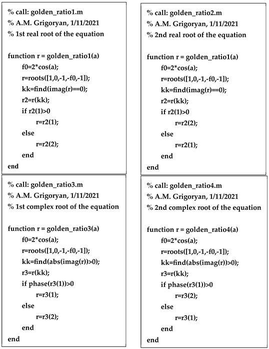
The authors declare no conflicts of interest.

Appendix A

The MATLAB R2022b based codes for computing the solutions, Φ k α ,   k = 1,4 , of the golden equation are given below. The following functions are used to compute these solutions:
(1)
golden_ratio1.m (for Φ 1 α , given an angle α ),
(2)
golden_ratio2.m (for Φ 2 α , given an angle α ),
(3)
golden_ratio3.m (for Φ 3 α , given an angle α ),
(4)
golden_ratio4.m (for Φ 4 α , given an angle α ).
Mathematics 13 00699 i002

References

  1. Stakhov, A. The golden section and modern harmony mathematics. In Applications of Fibonacci Numbers; Springer: Dordrecht, The Netherlands, 1998; Volume 7, pp. 393–399. [Google Scholar]
  2. Bradley, S. A geometric connection between generalized Fibonacci sequences and nearly golden sections. Fibonacci Q. 1999, 38, 174–180. [Google Scholar] [CrossRef]
  3. Antonelli, P.; Leandro, C.; Rutz, S. Mario Livio-The Golden Ratio The Story of PHI, the World’s Most Astonishing Number-Broadway Books (2003); Crown: New York, NY, USA, 2016. [Google Scholar]
  4. Timerding, H.E. Der Goldene Schnitt, 1999; The Digital Collection; University of Michigan Historical Math Collection; University of Michigan: Ann Arbor, MI, USA, 2025. [Google Scholar]
  5. Vorobiev, N. The Fibonacci Numbers, 2nd ed.; Nauka: Moscow, Russia, 1964. [Google Scholar]
  6. Herz-Fischler, R. The Shape of the Great Pyramid; Wilfrid Laurier University Press: Waterloo, ON, Canada, 2000. [Google Scholar]
  7. Van Zanten, A. The golden ratio in the arts of painting, building and mathematic. Nieuw Arch. Wisk. 1999, 17, 229–245. [Google Scholar]
  8. Olariu, A. Golden Section and the Art of Painting; National Institute for Physics and Nuclear Engineering: Bucharest, Romania, 1999; pp. 1–4. [Google Scholar]
  9. Grigoryan, A.M.; Agaian, S.S. Evidence of golden and aesthetic proportions in colors of paintings of the prominent artists. IEEE Multimedia 2020, 27, 8–16. [Google Scholar] [CrossRef]
  10. Kazlacheva, Z.; Ilieva, J. The golden and Fibonacci geometry in fashion and textile design. Proc. eRA 2016, 10, 15–64. [Google Scholar]
  11. Chan, J.Y.; Chang, G.H. The golden ratio optimizes cardiomelic form and function. J. Med. Hypotheses Ideas 2009, 3, 2. [Google Scholar]
  12. Henein, M.Y.; Zhao, Y.; Nicoll, R.; Sun, L.; Khir, A.W.; Franklin, K.; Lindqvist, P.; Golden Ratio Collaborators. The human heart: Application of the golden ratio and angle. Int. J. Cardiol. 2011, 150, 239–242. [Google Scholar] [CrossRef] [PubMed]
  13. Hassaballah, M.; Murakami, K.; Ido, S. Face detection evaluation: A new approach based on the golden ratio. Signal Image Video Process. 2013, 7, 307–316. [Google Scholar] [CrossRef]
  14. Grigoryan, A.M.; Agaian, S.S. Monotonic sequences for image enhancement and segmentation. Digit. Signal Process. 2015, 41, 70–89. [Google Scholar] [CrossRef]
  15. Nave, F.L.; Mazur, B. Reading Bombelli. Math. Intell. 2002, 24, 12–21. [Google Scholar] [CrossRef]
  16. Katz, V.J. A History of Mathematics; Addison Wesley: Boston, MA, USA, 2004; p. 220. Available online: https://archive.org/details/historyofmathema0000katz (accessed on 12 January 2025).
  17. Nickalls, R.W.D. Viète, Descartes, and the cubic equation. Math. Gaz. 2006, 90, 203–208. [Google Scholar] [CrossRef]
  18. Press, W.H.; Teukolsky, S.A.; Vetterling, W.T.; Flannery, B.P. Section 5.6 Quadratic and Cubic Equations, Numerical Recipes: The Art of Scientific Computing, 3rd ed.; Cambridge University Press: New York, NY, USA, 2007. [Google Scholar]
  19. Cardano’s Ars Magna in 1545 (Boyer and Merzbach 1991, p. 283). Available online: https://archive.org/details/arsmagnaorruleso0000card (accessed on 15 February 2025).
  20. Nielsen, M.; Chuang, I. Quantum Computation and Quantum Information, 2nd ed.; Cambridge UP: Cambridge, UK, 2001. [Google Scholar]
Figure 1. The partitioning of the interval according to the golden ratio rule.
Mathematics 13 00699 g001
Figure 2. (a) A five-sided polygon with a pentagram and (b) a golden isosceles triangle.
Mathematics 13 00699 g002
Figure 3. (a) A right triangle with the golden ratio property and (b) a triangle of the vertical cross-section of the pyramid of Cheops.
Mathematics 13 00699 g003
Figure 4. (a) The golden pair of vectors and these vectors with (b) the parallelograms and (c) triangles.
Mathematics 13 00699 g004
Figure 5. The vector a = [ 3,2 ] and its four similarity vectors.
Mathematics 13 00699 g005
Figure 6. The golden pairs { a 1 , a 2 } , { a 1 , a 3 } , and { a 2 , a 3 } .
Mathematics 13 00699 g006
Figure 7. The graphs of the polynomial and lines, when (a) α = 45 ° , (b) α = 100 ° , and (c) α = 30 ° .
Mathematics 13 00699 g007
Figure 8. The positive functions (a) D ( α ) and (b) v ( α ) for the Ferrari’s solution of the depressed equation.
Mathematics 13 00699 g008
Figure 9. The graphs of the four roots of Equation (9).
Mathematics 13 00699 g009
Figure 10. Polar plots of magnitudes of four roots, x k α ,   k = 1 : 4 , of Equation (9).
Mathematics 13 00699 g010
Figure 11. The polar plots of the sum of two roots: (a) x 1 α + x 2 α , (b) x 2 α + x 3 α , and (c) x 1 α + x 3 α .
Mathematics 13 00699 g011
Figure 12. (a) Two real solutions of Equation (9), (b) their sum, and (c) product.
Mathematics 13 00699 g012
Figure 13. (a) The sum of real solutions and the cosine function and (b) their difference.
Mathematics 13 00699 g013
Figure 14. The general golden ratio function Φ α ,   α [ 0,2 π ] .
Mathematics 13 00699 g014
Figure 15. The general golden ratio function and the function y ( α ) .
Mathematics 13 00699 g015
Figure 16. The general golden ratio function Φ α ,   α 0,2 π , with a few marked values on it.
Mathematics 13 00699 g016
Figure 17. The complex solution Φ 3 α ,   α 0,2 π : (a) the real part, (b) the imaginary part, and (c) the magnitude and its approximation F α .
Mathematics 13 00699 g017
Figure 18. Polar plots of three roots in absolute scale: (a) Φ 1 α ,   (b) Φ 2 α , and (c) Φ 3 α ,   a 0,2 π .
Mathematics 13 00699 g018
Figure 19. 2D vectors.
Mathematics 13 00699 g019
Figure 21. The parallelogram composed of the sum of two vectors (a) before and (b) after rotating by the angle of φ .
Mathematics 13 00699 g021
Figure 22. The sum of similarity sets for the 2D vectors (a) a 1 = [ 1,2 ] , a 2 = [ 1,3 ] and (b) a 1 = [ 2 , 3 ] , a 2 = 1,5 .
Mathematics 13 00699 g022
Figure 23. The sum of similarity sets for the 2D vectors (a) a 1 = [ 0,1 ] , a 2 = 1,0 , (b) a 1 = [ 1,2 ] , a 2 = 0 , 1 , and (c) a 1 = [ 2,3 ] , a 2 = 1 , 2 .
Mathematics 13 00699 g023
Figure 24. The unit vector e in the 3D spherical coordinate system.
Mathematics 13 00699 g024
Figure 25. The geometry of the similarity sets of the golden vectors with the 3D vectors (a) [0,0,1] and (b) [1,0,0].
Mathematics 13 00699 g025
Figure 26. The view with AZ = 0 and EL = 90 degrees of the geometry of similarity sets of the golden vectors with the 3D vectors (a) [0,0,1] and (b) [1,0,0].
Mathematics 13 00699 g026
Figure 27. The view with AZ = 0 and EL = 180 degrees: The geometry of the similarity sets of the golden vectors with the 3D vectors (a) [0,0,1] and (b) [1,0,0].
Mathematics 13 00699 g027
Figure 28. The 3D surface of the similarity sets of the golden vectors with the 3D vectors (a) [0,0,1] and (b) [1,0,0].
Mathematics 13 00699 g028
Figure 29. (a) Triangle for the vector V and (b) the triangle with the vertex a at the origin.
Mathematics 13 00699 g029
Figure 30. Five unit triangles with the angle λ = 40 ° .
Mathematics 13 00699 g030
Figure 31. The unit triangles with the angle (a) λ = 60 ° and (b) λ = 110 ° .
Mathematics 13 00699 g031
Figure 32. (a) The original triangle with angle θ = 33.69 ° and similarity triangles with the angle ϕ of (b) 20 ° , (c) 40 ° , and (d) 70 ° .
Mathematics 13 00699 g032
Figure 33. The similarity triangles for (a) the triangle with angle θ = 56.31 ° and (b) the triangle with angle θ = 45 ° .
Mathematics 13 00699 g033
Figure 34. The similarity triangles for the equilateral triangle, when the angle (a) λ = 60 ° and (b) λ = 30 ° .
Mathematics 13 00699 g034
Figure 35. (a) The original and rotated triangles, (b) the original triangle and its two pairs, and (c) the same shaded triangles.
Mathematics 13 00699 g035
Figure 36. The pentagon and its golden pairs for the angles (a) 72 ° , (b) 90 ° , (c) 160 ° , and (d) 275 ° .
Mathematics 13 00699 g036
Figure 37. The heptagon and its golden pairs for the angles (a) 30 ° , (b) 140 ° , (c) −100 ° , and (d) 200 ° .
Mathematics 13 00699 g037
Figure 38. The heptagram and its golden pairs for the angles (a) 30 ° , (b) 90 ° , (c) 160 ° , and (d) 220 ° .
Mathematics 13 00699 g038
Figure 39. (a) The enneagram and its golden pairs for the angles (b) 90 ° , (c) 160 ° , and (d) 220 ° .
Mathematics 13 00699 g039
Figure 40. The cross together with (a) 10 equal small crosses, (b) 10 golden pairs, and (c) 12 golden pairs.
Mathematics 13 00699 g040
Figure 41. The star together with (a) 12 equal small stars and (b) 12 stars of the golden pairs.
Mathematics 13 00699 g041
Figure 42. The (a) 7-pointed and (b) 9-pointed stars together with 12 stars of the golden pairs.
Mathematics 13 00699 g042
Figure 43. The 108-points on the Archimedes spiral together with 8 golden-pairs.
Mathematics 13 00699 g043
Figure 44. The 2D view of 108 golden (a) squares, (b) pentagons, (c) hexagons, and (d) heptagons.
Mathematics 13 00699 g044
Figure 45. 3D composition of golden figures for (a) the square and (b) the dodecagon.
Mathematics 13 00699 g045
Disclaimer/Publisher’s Note: The statements, opinions and data contained in all publications are solely those of the individual author(s) and contributor(s) and not of MDPI and/or the editor(s). MDPI and/or the editor(s) disclaim responsibility for any injury to people or property resulting from any ideas, methods, instructions or products referred to in the content.

