New Approximation Formula of Digamma Function with Bounded Remainder

Abstract

This study establishes the new approximation formula for the Digamma function $\psi \left(s\right)=lns-{\displaystyle \frac{1}{2s}}-{\displaystyle \frac{1}{12s\sqrt{s^2+\theta \left(s\right)}}},{\displaystyle \frac{1}{36}}<\theta \left(s\right)<{\displaystyle \frac{1}{5}};s>0$, as well as some of its inequalities, where $\theta \left(s\right)$ is a continuous function. We demonstrate numerically that our results are superior to some recent results.

1. Introduction

The logarithmic derivative of the Gamma function

$$\psi \left(s\right)={\displaystyle \frac{d}{ds}}ln\mathsf{\Gamma }\left(s\right),s>0$$

(1)

is known as the Digamma function and is used extensively in many mathematical and scientific contexts, where $\mathsf{\Gamma }$ is the Euler Gamma function. In analytic number theory, the Digamma function appears in the study of zeta functions and special values of L-functions, which have implications for understanding the distribution of prime numbers [1,2]. It is important in quantum field theory and statistical mechanics, particularly in evaluating sums and series that arise in particle interactions and quantum states [3]. Its connection to the Gamma function makes it essential in computations involving energy levels and decay rates in quantum systems. In statistics, it is used for deriving properties of distributions, particularly in the calculation of expectations and variances for the Gamma and related distributions [4]. It is also used in parameter estimation methods, such as maximum likelihood estimation for models involving the Gamma and Dirichlet distributions. In computational mathematics, the Digamma function is useful for evaluating infinite series and products, as well as for solving certain differential Equations [5]. Some of its special characteristics, including the recurrence relation

$$\psi (s+1)=\psi \left(s\right)+{\displaystyle \frac{1}{s}},$$

(2)

make it easier to simplify complicated formulas and derive some asymptotic approximations [1,6]. One area of research focuses on inequalities involving the Digamma function, which has several applications.

There are many researchers who have been interested in presenting inequalities for the digamma function. For example, in 1997, Anderson and Qiu [7] presented the doubly inequality

$$lns-{\displaystyle \frac{1}{s}}<\psi \left(s\right)<lns-{\displaystyle \frac{1}{2s}},s>0.$$

(3)

In 2000, Elezović, Giordano and Pečarić [8] proved that

$$ln(s+c_1)-{\displaystyle \frac{1}{s}}<\psi \left(s\right)<ln(s+c_2)-{\displaystyle \frac{1}{s}},s>0$$

(4)

where $c_1=1/2$ and $c_2=e^{-\gamma }$, where $\gamma =0.57721566\dots$ is the Euler–Mascheroni constant. After that, in 2014, Guo and Qi [9] proved that the scalars $c_1$ and $c_2$ are sharp. It is clear that the left-hand side of inequality (4) is better than the left-hand side of inequality (3).

In 2002, Allasia, Giordano and Pečarić [10], among other things, presented the following

$$-\sum _{i=1}^{2r}{\displaystyle \frac{(2^{1-2r}-1)B_{2r}}{2r{(s-1/2)}^{2r}}}<\psi \left(s\right)-ln(s-1/2)<-\sum _{i=1}^{2r+1}{\displaystyle \frac{(2^{1-2r}-1)B_{2r}}{2r{(s-1/2)}^{2r}}},s>1/2;r=0,1,2,\dots$$

(5)

where $B_r$ are the Bernoulli numbers generated by

$$\sum _{r=0}^{\infty }{\displaystyle \frac{B_r}{r!}}{t}^r=1-{\displaystyle \frac{t}{2}}+\sum _{r=1}^{\infty }{\displaystyle \frac{B_{2r}}{\left(2r\right)!}}{t}^{2r}={\displaystyle \frac{t}{e^t-1}},\left|t\right|<2\pi .$$

(6)

In 2005, Batir [11] showed that

$$\psi \left(s\right)\le ln(s-c_3),s\ge 1$$

(7)

and

$$\psi \left(s\right)>ln(s-c_4),s>1/2$$

(8)

with sharp scalars $c_3=1-e^{-\gamma }$ and $c_4=1/2$. Also, he proved that

$$ln2-ln(e^{1/s}-1)<\psi \left(s\right)<-ln(e^{1/s}-1),s>0$$

(9)

and

$$\psi \left(s\right)>ln{\displaystyle \frac{{\pi }^2}{6}}-\gamma -ln(e^{1/s}-1),s\ge 2.$$

(10)

In 2010, Mortici [12] showed that

$$ln(s+1/2)-{\displaystyle \frac{1}{s}}<\psi \left(s\right)<ln(s+1/2)-{\displaystyle \frac{1}{s}}+c_5,s>0$$

(11)

with sharp scalar $c_5=1-ln{\displaystyle \frac{3}{2}}-\gamma$. Also, he [13] proved that

$$ln(s+(3-\sqrt{3})/6)-{\displaystyle \frac{\sqrt{3}}{6s+3-\sqrt{3}}}-c_6<\psi (s+1)<ln(s+(3-\sqrt{3})/6)-{\displaystyle \frac{\sqrt{3}}{6s+3-\sqrt{3}}},s>0$$

(12)

and

$$ln(s+(3+\sqrt{3})/6)-{\displaystyle \frac{\sqrt{3}}{6s+3+\sqrt{3}}}-c_7<\psi (s+1)<ln(s+(3+\sqrt{3})/6)-{\displaystyle \frac{\sqrt{3}}{6s+3+\sqrt{3}}},s>0$$

(13)

where $c_6=0.00724\dots$ and $c_7=0.00269\dots$.

In 2011, Batir [14] presented

$${\displaystyle \frac{1}{2}}ln(s^2+s+c_8)<\psi (s+1)<{\displaystyle \frac{1}{2}}ln(s^2+s+c_9),s>0.$$

(14)

where $c_8=e^{-2\gamma }$ and $c_9=1/3$ are sharp scalars.

In 2016, Sun, Liu, Li and Zheng [15] presented

$${\displaystyle \frac{1}{24\left(s^2+s+\frac{17}{40}\right)}}+ln\left(s+c_{10}\right)<\psi (s+1)<{\displaystyle \frac{1}{24\left(s^2+s+\frac{17}{40}\right)}}+ln\left(s+c_{11}\right),s\ge 0$$

(15)

where the scalars $c_{10}=1/2$ and $c_{11}=e^{-\gamma -{\displaystyle \frac{5}{51}}}$ are sharp,

$$\psi (s+1)<{\displaystyle \frac{1}{24\left(s^2+s+\frac{17}{40}\right)}}+ln\left(s+1/2\right)+ln\left({\displaystyle \frac{c_{12}{e}^{-\frac{1}{24\left(s^2+s+\frac{17}{40}\right)}}}{2s+1}}+1\right),s\ge 0$$

(16)

where the scalar $c_{12}=2e^{-\gamma }-e^{5/51}$ is sharp,

$$\psi (s+1)<{\displaystyle \frac{1}{24\left(s^2+s+\frac{17}{40}\right)}}+ln\left(s+1/2\right)+c_{13},s\ge 0$$

(17)

where the scalar $c_{13}=ln2-5/51-\gamma$ is sharp, and

$${\displaystyle \frac{1}{24\left(s^2+s+\frac{17}{40}\right)}}-log\left(e^{q\left(s\right)}-1\right)+c_{14}<\psi (s+1)<{\displaystyle \frac{1}{24\left(s^2+s+\frac{17}{40}\right)}}-log\left(e^{q\left(s\right)}-1\right)+c_{15},s\ge 0$$

(18)

where the scalars $c_{14}=ln(e^{5347/4947}-1)-5/51-\gamma$ and $c_{15}=0$ are sharp, where

$$q\left(s\right)={\displaystyle \frac{4800s^4+19200s^3+28480s^2+18560s+5347}{3(s+1)\left(40s^2+40s+17\right)\left(40s^2+120s+97\right)}}.$$

For some recent results, inequalities, properties, and approximations for the Polygamma functions ${\psi }^{\left(n\right)}\left(s\right)$, $n=0,1,2,\dots$, we refer to [16,17,18,19,20] and the references therein. Overall, researchers studying mathematics and applied sciences benefit greatly from the new inequalities pertaining to the Digamma function, which gives accurate approximations and deeper understanding of the behavior of special functions.

In light of the previously described results, this study aims to offer the following Digamma formula

$$\psi \left(s\right)=lns-{\displaystyle \frac{1}{2s}}-{\displaystyle \frac{1}{12s\sqrt{s^2+\theta \left(s\right)}}},{\displaystyle \frac{1}{36}}<\theta \left(s\right)<{\displaystyle \frac{1}{5}};s>0$$

where $\theta \left(s\right)$ is a continuous function since

$$\theta \left(s\right)={\left(12s\left({\displaystyle \frac{1}{2s}}-lns+\psi \left(x\right)\right)\right)}^{-2}-s^2$$

and the function ${\displaystyle \frac{1}{2s}}-lns+\psi \left(x\right)$ is continuous and has no zeros for $s>0$. In this formula, our upper bound of $\psi (s+1)$ outperforms their upper bounds in the inequalities (15)–(17) for $s\ge 1$, and (18) for $s\ge 4$, numerically.

2. Main Results

In this section, we will need to introduce some auxiliary inequalities for the psi function, which depend on Padé approximants, to complete the proof of the main results.

Lemma 1.

The following inequality holds

$${\psi }^{\prime }\left(s\right)>{\displaystyle \frac{630s^5+315s^4+1155s^3+525s^2+274s+60}{30s^2\left(21s^4+35s^2+4\right)}},s>0.$$

(19)

Proof. 

Consider the function

$$T_1\left(s\right)={\psi }^{\prime }\left(s\right)-{\displaystyle \frac{630s^5+315s^4+1155s^3+525s^2+274s+60}{30s^2\left(21s^4+35s^2+4\right)}},s>0.$$

Using the derivative of the relation (2), we get the following

$$T_1\left(s\right)-T_1(s+1)={\displaystyle \frac{120}{s^2{(s+1)}^2\left(21s^4+35s^2+4\right)(7s(s+2)(3s(s+2)+11)+60)}}>0,s>0.$$

Then

$$T_1\left(s\right)>T_1(s+1)>T_1(s+2)>\cdots >T_1(s+r),r\in \mathbb{N}$$

but using the derivative of the asymptotic expansion [1]

$$\psi \left(s\right)\sim lns-{\displaystyle \frac{1}{s}}-\sum _{r=1}^{\infty }{\displaystyle \frac{B_r}{r{s}^r}},s\to \infty$$

(20)

where $B_r$ are the Bernoulli numbers, we have

$$\begin{array}{ccc}& & T_1\left(s\right)=\psi \left(s\right)-{\displaystyle \frac{s^{-6}}{630}}(630s^5+315s^4+1155s^3+525s^2+274s+60){\displaystyle \frac{1}{1+\frac{35s^2+4}{21s^4}}}\hfill \\ & & \sim {\displaystyle \frac{1}{s}}+{\displaystyle \frac{1}{s^2}}+\sum _{r=1}^{14}{\displaystyle \frac{B_r}{s^{r+1}}}+{\displaystyle \frac{s^{-6}}{630}}(630s^5+315s^4+1155s^3+525s^2+274s+60)\hfill \\ & & \left(1-{\displaystyle \frac{5}{3s^2}}+{\displaystyle \frac{163}{63s^4}}-{\displaystyle \frac{755}{189s^6}}+{\displaystyle \frac{24469}{3969s^8}}-{\displaystyle \frac{113285}{11907s^{10}}}+{\displaystyle \frac{3671347}{250047s^{12}}}-{\displaystyle \frac{16997315}{750141s^{14}}}\right)+\dots \hfill \\ & & \sim {\displaystyle \frac{40}{1617s^{11}}}-{\displaystyle \frac{1000}{5733s^{13}}}+{\displaystyle \frac{9680}{9261s^{15}}}+\dots ,s\to \infty \hfill \end{array}$$

and therefore, ${lim}_{s\to \infty }{T}_1\left(s\right)={lim}_{s\to \infty }\left({\displaystyle \frac{40}{1617s^{11}}}-{\displaystyle \frac{1000}{5733s^{13}}}+{\displaystyle \frac{9680}{9261s^{15}}}+O\left(s^{-17}\right)\right)=0$. Hence $T_1\left(s\right)>0$ for $s>0$, which completes the proof. □

Lemma 2.

The function

$$T_2\left(s\right)=s^2{\psi }^{\prime }\left(s\right)-s-{\displaystyle \frac{1}{2}}$$

(21)

is strictly completely monotonic, that is

$${(-1)}^r{T}_2^{\left(r\right)}\left(s\right)>0,r=0,1,2,\dots ;s>0.$$

Proof. 

Using the integral representation [1]

$$\psi \left(s\right)={\int }_0^{\infty }\left({\displaystyle \frac{e^{-t}}{t}}-{\displaystyle \frac{e^{-st}}{1-e^{-t}}}\right)dt,s>0$$

(22)

we get the following

$$\begin{array}{ccc}\hfill T_2\left(s\right)& =& {\int }_0^{\infty }{\displaystyle \frac{e^t\left(e^t(t-2)+t+2\right)}{{\left(e^t-1\right)}^3}}{e}^{-st}dt,s>0\hfill \\ & =& {\int }_0^{\infty }{\displaystyle \frac{e^t\left({\sum }_{m=3}^{\infty }\frac{(m-2)t^m}{m!}\right)}{{\left(e^t-1\right)}^3}}{e}^{-st}dt.\hfill \end{array}$$

Then,

$${\displaystyle \frac{d^r}{d{s}^r}}{T}_2\left(s\right)={(-1)}^r{\int }_0^{\infty }{\displaystyle \frac{e^t\left({\sum }_{m=3}^{\infty }\frac{(m-2)t^m}{m!}\right)}{{\left(e^t-1\right)}^3}}{t}^r{e}^{-st}dt,r=0,1,2,\dots ;s>0$$

which completes the proof. □

For some properties of completely monotonic functions and its various examples, including some special functions, we refer to [21,22] and the references therein.

Theorem 1.

The function

$$F\left(s\right)=\psi \left(s\right)-lns+{\displaystyle \frac{1}{2s}}+{\displaystyle \frac{1}{12s\sqrt{s^2+\frac{1}{5}}}}$$

is increasing for $s>0$. Moreover,

$$\psi \left(s\right)<lns-{\displaystyle \frac{1}{2s}}-{\displaystyle \frac{1}{12s\sqrt{s^2+\frac{1}{5}}}},s>0.$$

(23)

Proof. 

Using inequality (19), we have

$$\begin{array}{ccc}\hfill F^{\prime }\left(s\right)& =& {\psi }^{\prime }\left(s\right)-{\displaystyle \frac{1}{s}}-{\displaystyle \frac{1}{2s^2}}-{\displaystyle \frac{\sqrt{5}\left(10s^2+1\right)}{12s^2{\left(5s^2+1\right)}^{3/2}}}\hfill \\ & >& {\displaystyle \frac{K_1\left(s\right)}{60s^2{\left(5s^2+1\right)}^{3/2}\left(21s^4+35s^2+4\right)}}\hfill \end{array}$$

where

$$K_1\left(s\right)=-20\sqrt{5}-1050\sqrt{5}{s}^6-1855\sqrt{5}{s}^4-375\sqrt{5}{s}^2+\left(1050s^5+1750s^3+308s\right)\sqrt{5s^2+1}.$$

If

$$K_2\left(s\right)={\displaystyle \frac{1050\sqrt{5}{s}^6+1855\sqrt{5}{s}^4+375\sqrt{5}{s}^2+20\sqrt{5}}{\sqrt{5s^2+1}\left(1050s^5+1750s^3+308s\right)}},$$

then

$$K_2^{\prime }\left(s\right)={\displaystyle \frac{5\sqrt{5}{K}_3(s+1)}{14s^2{\left(5s^2+1\right)}^{5/2}{\left(15s^2+22\right)}^2}}$$

with

$$K_3(s+1)=6165s^6+\mathrm{36,990}{s}^5+\mathrm{97,536}{s}^4+\mathrm{143,544}{s}^3+\mathrm{122,551}{s}^2+\mathrm{56,654}s+\mathrm{10,848}.$$

Therefore, $K_2\left(s\right)$ is increasing for $s>1$ with ${lim}_{s\to \infty }{K}_2\left(s\right)=1$, and hence, $K_2\left(s\right)<1$ for $s\ge 1$. Then, $K_1\left(s\right)>0$ and $F\left(s\right)$ is increasing for $s\ge 1$.

Using Lemma 2, the function $T_2\left(s\right)$ is strictly decreasing and convex with tangent at $s=1$, given by

$$L_1\left(s\right)=(s-1)\left({\displaystyle \frac{{\pi }^2}{3}}-1+{\psi }^{″}\left(1\right)\right)+{\displaystyle \frac{1}{6}}\left({\pi }^2-9\right),$$

and hence,

$$T_2\left(s\right)>L_1\left(s\right),0\le s<1.$$

(24)

Also, consider the function

$$K_4\left(s\right)={\displaystyle \frac{\sqrt{5}\left(10s^2+1\right)}{12{\left(5s^2+1\right)}^{3/2}}}.$$

Then, the two functions $s(1-s)L_1\left(s\right)$ and $s(1-s)K_4\left(s\right)$ are concave down for $0\le x\le 1$ and pass through the points $(0,0)$ and $(1,0)$, where

$${\displaystyle \frac{d^2}{d{s}^2}}\left(s(1-s)L_1\left(s\right)\right)=-6s\left({\displaystyle \frac{{\pi }^2}{3}}-1+{\psi }^{″}\left(1\right)\right)+{\displaystyle \frac{1}{3}}\left(9-{\pi }^2\right)+4\left({\displaystyle \frac{{\pi }^2}{3}}-1+{\psi }^{″}\left(1\right)\right)$$

and

$${\displaystyle \frac{d^2}{d{s}^2}}\left(s(1-s)K_{1}4\left(s\right)\right)={\displaystyle \frac{\sqrt{5}(5s(s(20(s-3)s-13)+3)-2)}{12{\left(5s^2+1\right)}^{7/2}}}.$$

Also, ${\left.{\displaystyle \frac{d}{ds}}\left(s(1-s)L_1\left(s\right)\right)\right|}_{s=0}>{\left.{\displaystyle \frac{d}{ds}}\left(s(1-s)L_1\left(s\right)\right)\right|}_{s=0}$ and ${\left.{\displaystyle \frac{d}{ds}}\left(s(1-s)L_1\left(s\right)\right)\right|}_{s=1}<{\left.{\displaystyle \frac{d}{ds}}\left(s(1-s)L_1\left(s\right)\right)\right|}_{s=1}$. Therefore,

$$L_1\left(s\right)>K_4\left(s\right),0\le s<1.$$

(25)

From inequalities (24) and (25), we have

$$s^2{\psi }^{\prime }\left(s\right)-s-{\displaystyle \frac{1}{2}}>{\displaystyle \frac{\sqrt{5}\left(10s^2+1\right)}{12{\left(5s^2+1\right)}^{3/2}}},0\le s<1$$

or $F^{\prime }\left(s\right)>0$ for $0\le s<1$ and hence $F\left(s\right)$ is increasing function for $0\le s<1$.

Now, $F\left(s\right)$ is increasing for $s>0$ and using the asymptotic expansion (20), we have

$$F\left(s\right)\sim -{\displaystyle \frac{137}{50400s^6}}+{\displaystyle \frac{19}{4800s^8}}-{\displaystyle \frac{15923}{2112000s^{10}}}+{\displaystyle \frac{55262801}{2620800000s^{12}}}+\dots ,s\to \infty$$

and

$$\underset{s\to \infty }{lim}F\left(s\right)=0.$$

Hence, $F\left(s\right)<0$ for $s>0$, which completes the proof. □

Lemma 3.

The following inequality holds

$${\psi }^{\prime }\left(s\right)<{\displaystyle \frac{5s\left(3s\right(434s-191)+697)}{6\left(5s\right(s\left(s\right(217s-204)+182)-57)+27)}},s\ge 1.$$

(26)

Proof. 

Consider the function

$$P_1\left(s\right)={\psi }^{\prime }\left(s\right)-{\displaystyle \frac{5s\left(3s\right(434s-191)+697)}{6\left(5s\right(s\left(s\right(217s-204)+182)-57)+27)}}.$$

Using the derivative of the relation (2), we get the following

$$P_1\left(s\right)-P_1(s+1)={\displaystyle \frac{P_2\left(s\right)}{P_3\left(s\right)}},$$

where

$$P_2(s+1)=-108981-128340s$$

and

$$\begin{array}{ccc}\hfill P_3(s+1)& =& 8816949+70773648s+256372004s^2+553286170s^3\hfill \\ & +& 788740265s^4+775781940s^5+532313340s^6+251076450s^7\hfill \\ & +& 77766175s^8+14267750s^9+1177225s^{10}.\hfill \end{array}$$

Then,

$$P_1\left(s\right)-P_1(s+1)<0,s\ge 1$$

or

$$P_1\left(s\right)<P_1(s+1)<P_1(s+2)<\cdots <P_1(s+r)s\ge 1;r\in \mathbb{N}$$

but using the derivative of the asymptotic expansion (20), we have

$$P_1\left(s\right)\sim -{\displaystyle \frac{207}{15190s^8}}-{\displaystyle \frac{222533}{8240575s^9}}+{\displaystyle \frac{39787371}{3576409550s^{10}}}+{\displaystyle \frac{665202886653}{8536889595850s^{11}}}+\dots ,s\to \infty ,$$

and therefore, ${lim}_{s\to \infty }{P}_1\left(s\right)=0$. Hence, $P_1\left(s\right)<0$ for $s\ge 1$, which completes the proof. □

Theorem 2.

The function

$$M\left(s\right)=\psi \left(s\right)-lns+{\displaystyle \frac{1}{2s}}+{\displaystyle \frac{1}{12s\sqrt{s^2+\frac{1}{36}}}}$$

decreases for $s>0$. Moreover,

$$\psi \left(s\right)>lns-{\displaystyle \frac{1}{2s}}-{\displaystyle \frac{1}{12s\sqrt{s^2+\frac{1}{36}}}},s>0.$$

(27)

Proof. 

Using inequality (26), we have the following

$$\begin{array}{ccc}\hfill M^{\prime }\left(s\right)& =& {\psi }^{\prime }\left(s\right)-{\displaystyle \frac{1}{s}}-{\displaystyle \frac{1}{2s^2}}-{\displaystyle \frac{72s^2+1}{2s^2{\left(36s^2+1\right)}^{3/2}}}\hfill \\ & <& {\displaystyle \frac{P_4\left(s\right)}{6s^2{\left(36s^2+1\right)}^{3/2}{P}_5\left(s\right)}}\hfill \end{array}$$

where

$$\begin{array}{ccc}\hfill P_4(s+1)& =& -157023-926229s-2325792s^2-3218640s^3-2613615s^4-1185840s^5\hfill \\ & -& 234360s^6+\left(25049+119340s+244443s^2+269753s^3+158580s^4\right.\hfill \\ & +& \left.39060s^5\right)\sqrt{37+72s+36s^2}\hfill \end{array}$$

and

$$P_5(s+1)=1085s^4+3320s^3+4360s^2+2815s+717.$$

Now, the function

$$P_6\left(s\right)={\displaystyle \frac{-157023-926229s-2325792s^2-3218640s^3-2613615s^4-1185840s^5-234360s^6}{\left(25049+119340s+244443s^2+269753s^3+158580s^4+39060s^5\right)\sqrt{37+72s+36s^2}}}$$

is decreasing since

$$P_6^{\prime }\left(s\right)={\displaystyle \frac{-P_7\left(s\right)}{{(36s(s+2)+37)}^{3/2}{(s(5s(217s+447)+1908)+677)}^2}}$$

with

$$\begin{array}{ccc}\hfill P_7\left(s\right)& =& 8288949957+76937794806s+332247425724s^2+882585320958s^3\hfill \\ & +& 1599269941740s^4+2063028245130s^5+1912954553355s^6+1254252833280s^7\hfill \\ & +& 554394368520s^8+148659235200s^9+18308203200s^{10}.\hfill \end{array}$$

However, $P_6\left(0\right)=-{\displaystyle \frac{157023}{25049\sqrt{37}}}<-1$, then $P_4(s+1)<0$ for $s\ge 0$ and then $M\left(s\right)$ is decreasing for $s\ge 1$.

Using Lemma 2, the function $T_2\left(s\right)$ is convex, then the line segment that connects any two different points is located above the graph that connects the two points. Therefore,

$$T_2\left(s\right)<L_2\left(s\right)={\displaystyle \frac{1}{4}}\left(\left({\pi }^2-12\right)s+2\right),0\le s\le {\displaystyle \frac{1}{2}}$$

and

$$T_2\left(s\right)<L_3\left(s\right)={\displaystyle \frac{1}{12}}\left(\left({\pi }^2-12\right)s+{\pi }^2-6\right),{\displaystyle \frac{1}{2}}\le s\le 1.$$

Now, consider the function

$$P_8\left(s\right)={\displaystyle \frac{72s^2+1}{2{\left(36s^2+1\right)}^{3/2}}}.$$

Then,

$${\displaystyle \frac{d}{ds}}{\displaystyle \frac{L_2\left(s\right)}{P_8\left(s\right)}}={\displaystyle \frac{\sqrt{36s^2+1}\left({\pi }^2\left(72\left(72s^4+s^2\right)+1\right)-12\left(6s\left(12s\left(72s^2-6s+1\right)+1\right)+1\right)\right)}{2{\left(72s^2+1\right)}^2}},$$

and hence, the function ${\displaystyle \frac{L_2\left(s\right)}{P_8\left(s\right)}}$ has an absolute maximum at $s=0$ on the interval $[0,1/2]$ but ${\displaystyle \frac{L_2\left(0\right)}{P_8\left(0\right)}}=1$. Therefore,

$$L_2\left(s\right)<P_8\left(s\right),0\le s\le {\displaystyle \frac{1}{2}}.$$

(28)

Also,

$${\displaystyle \frac{d}{ds}}{\displaystyle \frac{P_8\left(s\right)}{L_3\left(s\right)}}={\displaystyle \frac{P_9\left(s\right)}{{\left(\left({\pi }^2-12\right)s+{\pi }^2-6\right)}^2{\left(36s^2+1\right)}^{5/2}}},$$

where

$$P_9\left(s\right)=\left(62208-5184{\pi }^2\right)s^4+\left(15552-2592{\pi }^2\right)s^3+\left(864-72{\pi }^2\right)s^2+\left(36{\pi }^2-216\right)s-{\pi }^2+12.$$

Hence, the function ${\displaystyle \frac{P_8\left(s\right)}{L_3\left(s\right)}}$ has absolute minimum at $s=s_0\approx 0.875586$ on the interval $[1/2,1]$ but ${\displaystyle \frac{P_8\left(s_0\right)}{L_3\left(s_0\right)}}>1$. Therefore,

$$P_8\left(s\right)>L_3\left(s\right),{\displaystyle \frac{1}{2}}\le s\le 1.$$

(29)

From inequalities (28) and (29), we have the following

$$s^2{\psi }^{\prime }\left(s\right)-s-{\displaystyle \frac{1}{2}}<{\displaystyle \frac{72s^2+1}{2{\left(36s^2+1\right)}^{3/2}}},0\le s<1$$

or $M^{\prime }\left(s\right)<0$ for $0\le s<1$, and hence, $M\left(s\right)$ is decreasing function for $0\le s<1$.

Now, $M\left(s\right)$ is decreasing for $s>0$ and using the asymptotic expansion (20), we have the following

$$M\left(s\right)\sim {\displaystyle \frac{31}{4320s^4}}-{\displaystyle \frac{1145}{290304s^6}}+{\displaystyle \frac{186599}{44789760s^8}}-{\displaystyle \frac{214990463}{28378791936s^{10}}}+\dots ,s\to \infty$$

and

$$\underset{s\to \infty }{lim}M\left(s\right)=0.$$

Hence, $M\left(s\right)>0$ for $s>0$, which completes the proof. □

As a consequence of the above results, we conclude the following Digamma function formula:

Theorem 3.

$$\psi \left(s\right)=lns-{\displaystyle \frac{1}{2s}}-{\displaystyle \frac{1}{12s\sqrt{s^2+\theta \left(s\right)}}},{\displaystyle \frac{1}{36}}<\theta \left(s\right)<{\displaystyle \frac{1}{5}};s>0.$$

(30)

3. Comparisons

Consider the following upper bounds of $\psi (s+1)$

$$U_1\left(s\right)={\displaystyle \frac{1}{24\left(s^2+s+\frac{17}{40}\right)}}+ln\left(s+e^{-\gamma -{\displaystyle \frac{5}{51}}}\right),s\ge 1$$

$$U_2\left(s\right)={\displaystyle \frac{1}{24\left(s^2+s+\frac{17}{40}\right)}}+ln\left({\displaystyle \frac{\left(2e^{-\gamma }-e^{5/51}\right)e^{-\frac{1}{24\left(s^2+s+\frac{17}{40}\right)}}}{2s+1}}+1\right)+ln\left(s+{\displaystyle \frac{1}{2}}\right),s\ge 1$$

$$U_3\left(s\right)={\displaystyle \frac{1}{24\left(s^2+s+\frac{17}{40}\right)}}+ln\left(s+{\displaystyle \frac{1}{2}}\right)-{\displaystyle \frac{5}{51}}-\gamma +ln\left(2\right),s\ge 1$$

$$U_4\left(s\right)={\displaystyle \frac{1}{24\left(s^2+s+\frac{17}{40}\right)}}-ln\left(exp\left({\displaystyle \frac{4800s^4+19200s^3+28480s^2+18560s+5347}{3(s+1)\left(40s^2+40s+17\right)\left(40s^2+120s+97\right)}}\right)-1\right),s\ge 1$$

and our new one

$$U_5\left(s\right)=ln\left(s\right)+{\displaystyle \frac{1}{2s}}-{\displaystyle \frac{1}{12s\sqrt{s^2+\frac{1}{5}}}},s\ge 1.$$

Figure 1, Figure 2, Figure 3 and Figure 4 show the numerical priority of our new bound $U_5\left(s\right)$ over $U_1\left(s\right),U_2\left(s\right)$, and $U_3\left(s\right)$ for $s\ge 1$ and over $U_4\left(s\right)$ for $s\ge 4$.

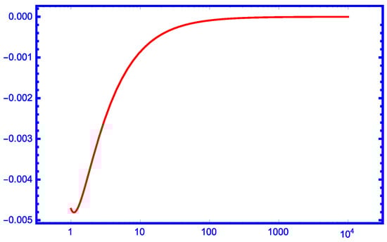
Figure 1. The function $U_5\left(s\right)-U_1\left(s\right)$ for $s\in [1,{10}^4]$.

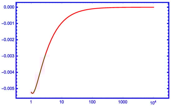
Figure 2. The function $U_5\left(s\right)-U_2\left(s\right)$ for $s\in [1,{10}^4]$.

Figure 3. The function $U_5\left(s\right)-U_1\left(s\right)$ for $s\in [1,{10}^4]$.

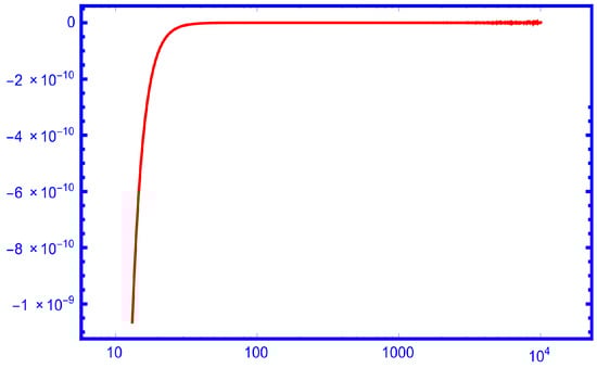
Figure 4. The function $U_5\left(s\right)-U_2\left(s\right)$ for $s\in [1,{10}^4]$.

4. Open Problem

For the two numbers a and b, the harmonic mean can be written as $H(a,b)={\displaystyle \frac{2ab}{a+b}}$. In 1974, Gautschi [23] established an inequality involving the gamma function $\mathsf{\Gamma }\left(s\right)$, where he specifically proved that the harmonic means of $\mathsf{\Gamma }\left(s\right)$ and $\mathsf{\Gamma }(1/s)$ satisfy that

$$H\left(\mathsf{\Gamma }\right(s),\mathsf{\Gamma }(1/s\left)\right)\ge 1,s>0$$

(31)

where the equality holds if and only if $s=1$. In 2017, Alzer and Jameson [24] showed that for all positive real numbers $s>0$, the harmonic mean of $\psi \left(s\right)$ and $\psi (1/s)$ satisfies

$$-\gamma \le H\left(\psi \right(s),\psi (1/s\left)\right),s>0$$

(32)

where the equality holds if and only if $s=1$. Also, Alzer [25] refined (32) by proving that

$${\displaystyle \frac{-2\gamma s}{s^2+1}}\le H(\psi \left(s\right),\psi (1/s)),s>0$$

(33)

where the equality holds if and only if $s=1$. In 2023, Nantomah, Abe-I-Kpeng and Sandow [26] extend the results to the trigamma function ${\psi }^{\prime }$ by presenting

$$H({\psi }^{\prime }\left(s\right),{\psi }^{\prime }(1/s))\le {\displaystyle \frac{{\pi }^2}{6}},s>0$$

(34)

where the equality holds if and only if $s=1$. For more results about the mean inequality for the generalized functions ${\mathsf{\Gamma }}_q\left(s\right)$, ${\psi }_q\left(s\right)$, and ${\psi }_k\left(s\right)$, we refer to the references [27,28,29,30].

We propose the following open problem for interested readers to discuss.

Open Problem: For the functions

$$U\left(x\right)=ln\left(x\right)-{\displaystyle \frac{1}{2x}}-{\displaystyle \frac{1}{12x\sqrt{x^2+\frac{1}{5}}}},$$

and

$$L\left(x\right)=ln\left(x\right)-{\displaystyle \frac{1}{2x}}-{\displaystyle \frac{1}{12x\sqrt{x^2+\frac{1}{36}}}},$$

we have

$$H\left(L\right(s),L(1/s\left)\right)\le H\left(\psi \right(s),\psi (1/s\left)\right)\le H\left(U\right(s),U(1/s\left)\right),s>0.$$

5. Discussion

The significance of the Digamma function and some of its applications in several fields of study have been explained. The main conclusions of this study are outlined in Theorem 3. More specifically, we gave a new approximation formula for the Digamma function with a bounded remainder, which is important for real-world computations since it presents bounds of the approximation error and yields new inequalities of $\psi \left(s\right)$. Lastly, we have numerically shown that our new method is superior compared to some recent results.

References

- Andrews, G.E.; Askey, R.A.; Roy, R. Special Functions; Encyclopedia of Mathematics and Its Applications 71; Cambridge University Press: Cambridge, UK, 1999. [Google Scholar]
- Apostol, T.M. Introduction to Analytic Number Theory; Springer: Berlin/Heidelberg, Germany, 2010. [Google Scholar]
- Moll, V.H. Special Integrals of Gradshteyn and Ryzhik: The Proofs-Volume II; Cambridge University Press: Cambridge, UK, 2020. [Google Scholar]
- Gradshteyn, I.S.; Ryzhik, I.M.; Jeffrey, A.; Zwillinger, D.; Moll, V. Table of Integrals, Series, and Products, 8th ed.; Academic Press: Cambridge, MA, USA, 2015. [Google Scholar]
- Olver, F.W.J.; Lozier, D.W.; Boisvert, R.F.; Clark, C.W. NIST Handbook of Mathematical Functions; Cambridge University Press: Cambridge, UK, 2010. [Google Scholar]
- Abramowitz, M.; Stegun, I.A. (Eds.) Handbook of Mathematical Functions with Formulas, Graphs, and Mathematical Tables, National Bureau of Standards; Applied Mathematics Series 55; 9th Printing; Dover Publications: New York, NY, USA; Washington, DC, USA, 1972. [Google Scholar]
- Anderson, G.D.; Qiu, S.L. A monotonicity property of the gamma function. Proc. Am. Math. Soc. 1997, 125, 3355–3362. [Google Scholar] [CrossRef]
- Elezović, N.; Giordano, C.; Pečarić, J. The best bounds in Gautschi’s inequalitity. Math. Inequal. Appl. 2000, 3, 239–252. [Google Scholar]
- Guo, B.-N.; Qi, F. Sharp inequalities for the psi function and harmonic numbers. Analysis 2014, 34, 1–10. [Google Scholar] [CrossRef][Green Version]
- Allasia, G.; Giordano, C.; Pečarić, J. Inequalities for the gamma function relating to asymptotic expasions. Math. Inequal. Appl. 2002, 5, 543–555. [Google Scholar]
- Batir, N. Some new inequalities for Gamma and Polygamma functions. J. Inequal. Pure Appl. Math. 2005, 6, 103. [Google Scholar]
- Mortici, C. Sharp bounds for gamma and digamma function arising from Burnside’s formula. Rev. Anal. Numer. Th. Approx. 2010, 39, 69–72. [Google Scholar] [CrossRef]
- Mortici, C. Estimating the digamma and trigamma functions by com- pletely monotonicity arguments. Appl. Math. Comp. 2010, 217, 4081–4085. [Google Scholar] [CrossRef]
- Batir, N. Sharp bounds for the psi function and harmonic numbers. Math. Inequal. Appl. 2011, 14, 917–925. [Google Scholar] [CrossRef]
- Sun, B.-C.; Liu, Z.-M.; Li, Q.; Zheng, S.-Z. The monotonicity and convexity of a function involving psi function with applications. J. Inequalities Appl. 2016, 2016, 151. [Google Scholar] [CrossRef]
- Mahmoud, M.; Almuashi, H. An Approximation Formula for Nielsen’s Beta Function Involving the Trigamma Function. Mathematics 2022, 10, 4729. [Google Scholar] [CrossRef]
- Mahmoud, M.; Almuashi, H. Two Approximation Formulas for Bateman’s G-Function with Bounded Monotonic Errors. Mathematics 2022, 10, 4787. [Google Scholar] [CrossRef]
- Qi, F.; Lim, D.; Nantomah, K. Monotonicity and positivity of several functions involving ratios and products of polygamma functions. J. Inequal. Appl. 2025, 5, 2025. [Google Scholar] [CrossRef]
- Qi, F.; Agarwal, R.P. Several Functions Originating from Fisher-Rao Geometry of Dirichlet Distributions and Involving Polygamma Functions. Mathematics 2024, 12, 44. [Google Scholar] [CrossRef]
- Yin, H.-P.; Han, L.-X.; Qi, F. Decreasing and complete monotonicity of functions defined by derivatives of completely monotonic function involving trigamma function. Demonstr. Demonstr. Math. 2024, 57, 20240041. [Google Scholar] [CrossRef]
- Widder, D.V. The Laplace Transform; Princeton University Press: Princeton, NJ, USA, 1946. [Google Scholar]
- Qi, F.; Wang, S.-H. Complete monotonicity, completely monotonic degree, integral representations, and an inequality related to the exponential, trigamma, and modified Bessel functions. Glob. J. Math. Anal. 2014, 2, 91–97. [Google Scholar] [CrossRef]
- Gautschi, W. A harmonic mean inequality for the gamma function. SIAM J. Math. Anal. 1974, 5, 278–281. [Google Scholar] [CrossRef]
- Alzer, H.; Jameson, G. A harmonic mean inequality for the digamma function and related results. Rend. Semin. Mat. Univ. Padova 2017, 137, 203–209. [Google Scholar] [CrossRef] [PubMed]
- Alzer, H. A Mean Value Inequality for the Digamma Function, Rendiconti Sem. Mat. Univ. Pol. Torino 2017, 75, 19–25. [Google Scholar]
- Nantomah, K.; Abe-I-Kpeng, G.; Sandow, S. On some properties of the Trigamma function. arXiv 2023, arXiv:2304.12081v1. [Google Scholar]
- Alzer, H.; Salem, A. A harmonic mean inequality for the q-gamma function. Ramanujan J. 2022, 58, 1025–1041. [Google Scholar] [CrossRef]
- Bouali, M. A harmonic mean inequality for the q-gamma and q-digamma functions. Filomat 2021, 35, 4105–4119. [Google Scholar] [CrossRef]
- Yildirim, E. Monotonicity Properties on k-Digamma Function and its Related Inequalities. J. Math. Inequal. 2020, 14, 161–173. [Google Scholar] [CrossRef]
- Yin, L.; Huang, L.-G.; Lin, X.-L.; Wang, Y.-L. Monotonicity, concavity, and inequalities related to the generalized digamma function. Adv. Differ. Equ. 2018, 2018, 246. [Google Scholar] [CrossRef]
Disclaimer/Publisher’s Note: The statements, opinions and data contained in all publications are solely those of the individual author(s) and contributor(s) and not of MDPI and/or the editor(s). MDPI and/or the editor(s) disclaim responsibility for any injury to people or property resulting from any ideas, methods, instructions or products referred to in the content. |
© 2025 by the authors. Licensee MDPI, Basel, Switzerland. This article is an open access article distributed under the terms and conditions of the Creative Commons Attribution (CC BY) license (https://creativecommons.org/licenses/by/4.0/).