
Optimizing Inventory for Imperfect and Gradually Deteriorating Items Under Multi-Level Trade Credit in a Sustainable Supply Chain

Abstract
:1. Introduction
2. Literature Review
2.1. Carbon Emission in Inventory Models
2.2. Non-Instantaneous Degrading Items in Inventory Management Models
2.3. Trade Credit in Inventory Models
2.4. Imperfect Within Inventory Models
3. Problem Description, Notation, and Assumptions
3.1. Problem Description
3.2. Notations
3.3. Assumptions
- i.
- There are carbon emissions and energy consumption per unit associated with storing inventory in warehouses. As a result, represents the holding cost related to carbon emissions per unit item.
- ii.
- is the rate of annual demand, which is known, uniform, and constant.
- iii.
- The distribution of the proportion of items of defective quality (p) is uniform in [α, β] where [0 ≤ α ≤ β ≤ 1].
- iv.
- There is a carbon emission cost on purchasing units from the supplier, which is paid by the retailer, as per government policy.
- v.
- The cost of carbon emissions when an item is ordered is .
- vi.
- Lead time is never changing. The replenishment rate occurs at an infinite rate.
- vii.
- A single item is used in the inventory model.
- viii.
- No shortages occur in the inventory model.
- ix.
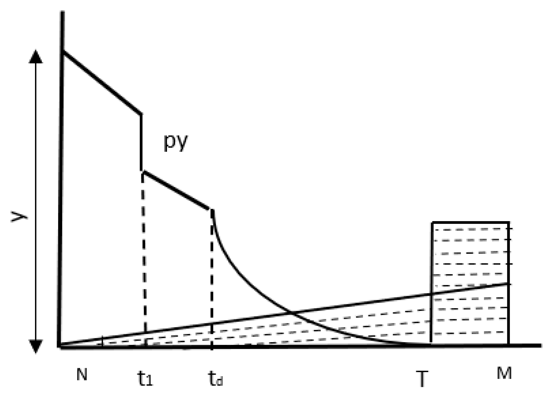
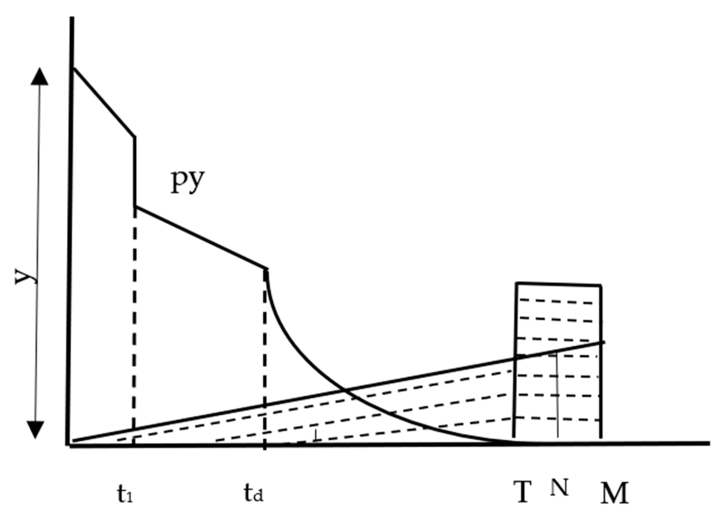
- The supplier’s (M) credit period is always greater than or equal to the retailer’s (N) credit duration for consumers. This relationship ensures M ≥ N.
- x.
- During case 1: , there is no interest charged. But in case 2: and case 3: , , the retailer will charge for those items that are left in stock.
- xi.
- Between periods N and M, the retailer earns a profit through credit financing. Earnings begin when customers start making payments and continue until the designated payment period for the goods expires.
4. Model Description and Analysis
- (a)
- Sale revenue
- (b)
- The cost of order cost
- (c)
- The cost of purchase
- (d)
- The cost to hold the inventory
- (e)
- The cost of deterioration
- (f)
- Screening cost
- (g)
- Further, on the basis of the credit periods M and N, the interest paid () and interest earned (IE) will be calculated as per the cases and subcases.
- (i)
- (ii)
- (iii)
- (1.1)
- (1.2)
- (1.3)
5. Solution Procedure
| Algorithm 1. Finding the optimal value T* |
| Step 1: Put values of all the parameters in Equation (A1) Step 2: Determine the value of cycle length, T. Now, using the value of T, calculate the values of y from Equation (8). (case 1: subcase 1.1 satisfy)) then the cycle length will be T and the value of expected total profit, E[TPU], can be obtained by putting T in Equation (A1), else this case is not feasible and set E[TPU] = 0. then find T and E[TPU] for this case from Equation (A1), else case is not possible, set E[TPU] = 0. If () Then determine T and E[TPU] from Equation (A1), else put E[TPU] = 0, in case of not feasible ) then calculate T and E[TPU] from Equation (A3), else E[TPU] = 0. then find T and predicted total profit E[TPU] from (A3) else put E[TPU] = 0. then determine T and E[TPU] from Equation (A5) else place E[TPU] = 0. ) then compute T and E[TPU] from (A6) else set E[TPU] = 0. ) then evaluate T and E[TPU] from (A6) else put E[TPU]= 0. ) then determine T and E[TPU] from Equation (A6) else put E[TPU] = 0. ) then evaluate T and E[TPU] from (A8) else in the case of not feasible, put E[TPU] = 0. Step 3. Compare the expected total profit for all the 10 cases, i.e., Max {for all cases E[TPU]i.j, (i = 1, 2, 3 and j = 1, 2, 3, 4, 5, 6} |
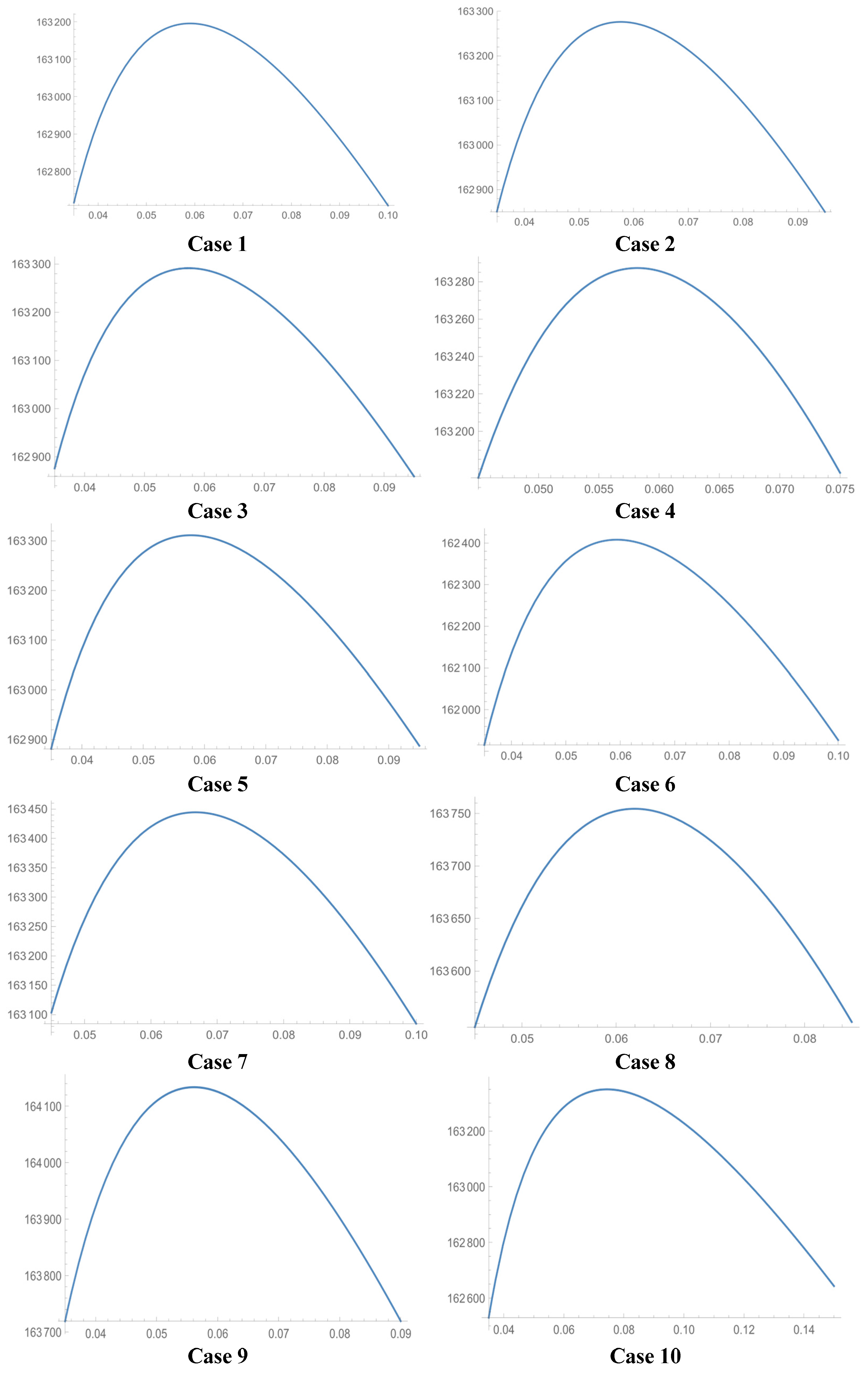
6. Numerical Example
7. Sensitivity Analysis
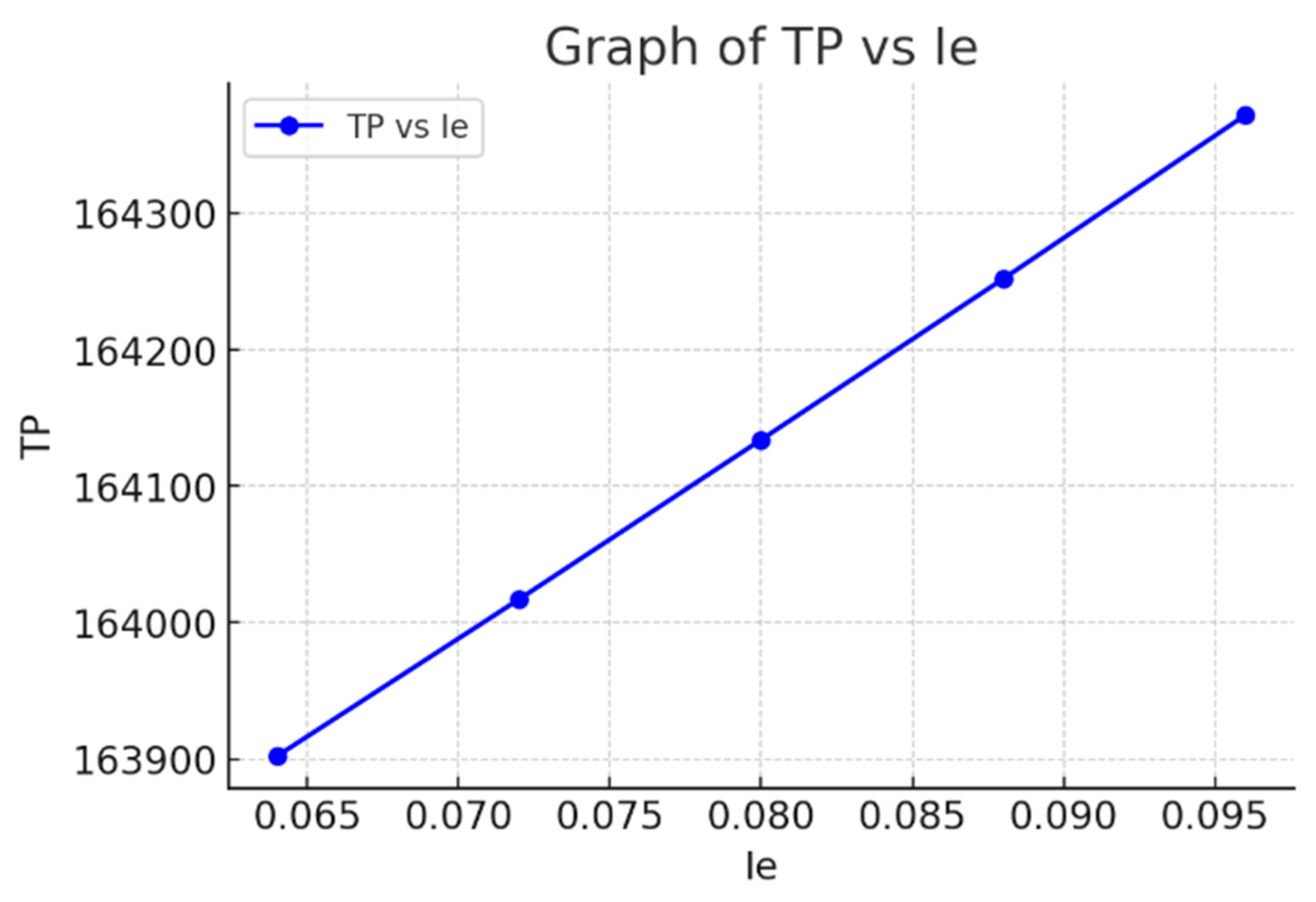
- As decreases, the processing time T gradually increases. This implies that higher interest rates may incentivize quicker or more efficient operations, likely due to better resource utilization.
- steadily declines as decreases. This decline indicates that lower interest earnings directly affect profitability, possibly due to reduced capital reinvestment benefits.
8. Managerial Implications
9. Concluding Remarks and Future Scope
Author Contributions
Funding
Data Availability Statement
Conflicts of Interest
Appendix A
References
- Ghare, P.M.; Schrader, G.F. An inventory model for exponentially deteriorating items. J. Ind. Eng. 1963, 14, 238–243. [Google Scholar]
- Alsaedi, B.S.; Alamri, O.A.; Jayaswal, M.K.; Mittal, M. A sustainable green supply chain model with carbon emissions for defective items under learning in a fuzzy environment. Mathematics 2023, 11, 301. [Google Scholar] [CrossRef]
- Alamri, O.A.; Lamba, N.K.; Jayaswal, M.K.; Mittal, M. A sustainable inventory model with advertisement effort for imperfect quality items under learning in fuzzy monsoon demand. Mathematics 2024, 12, 2432. [Google Scholar] [CrossRef]
- Jaggi, C.K.; Goel, S.K.; Mittal, M. Credit financing in economic ordering policies for defective items with allowable shortages. Appl. Math. Comput. 2013, 219, 5268–5282. [Google Scholar] [CrossRef]
- Sarkar, B.; Mahapatra, A.S. Periodic review fuzzy inventory model with variable lead time and fuzzy demand. Int. Trans. Oper. Res. 2017, 24, 1197–1227. [Google Scholar] [CrossRef]
- Shah, N.H.; Keswani, M.; Khedlekar, U.K.; Prajapati, N.M. Non-instantaneous controlled deteriorating inventory model for stock-price-advertisement dependent probabilistic demand under trade credit financing. Opsearch 2024, 61, 421–459. [Google Scholar] [CrossRef]
- Ahmed, W.; Sarkar, B. Impact of carbon emissions in a sustainable supply chain management for a second generation biofuel. J. Clean. Prod. 2018, 186, 807–820. [Google Scholar] [CrossRef]
- Sarkar, B.; Gupta, H.; Chaudhuri, K.; Goyal, S.K. An integrated inventory model with variable lead time, defective units and delay in payments. Appl. Math. Comput. 2014, 237, 650–658. [Google Scholar] [CrossRef]
- Dye, C.Y.; Yang, C.T. Sustainable trade credit and replenishment decisions with credit-linked demand under carbon emission constraints. Eur. J. Oper. Res. 2015, 244, 187–200. [Google Scholar] [CrossRef]
- Kazemi, N.; Abdul-Rashid, S.H.; Ghazilla, R.A.R.; Shekarian, E.; Zanoni, S. Economic order quantity models for items with imperfect quality and emission considerations. Int. J. Syst. Sci. Oper. Logist. 2018, 5, 99–115. [Google Scholar] [CrossRef]
- Tayyab, M.; Sarkar, B. Optimal batch quantity in a cleaner multi-stage lean production system with random defective rate. J. Clean. Prod. 2016, 139, 922–934. [Google Scholar] [CrossRef]
- Kim, S.J.; Sarkar, B. Supply Chain Model with Stochastic Lead Time, Trade-Credit Financing, and Transportation Discounts. Math. Probl. Eng. 2017, 2017, 6465912–6465925. [Google Scholar] [CrossRef]
- Sarkar, B.; Ahmed, W.; Kim, N. Joint effects of variable carbon emission cost and multi-delay-in-payments under single-setup-multiple-delivery policy in a global sustainable supply chain. J. Clean. Prod. 2018, 185, 421–445. [Google Scholar] [CrossRef]
- Ahmed, W.; Sarkar, B. Management of next-generation energy using a triple bottom line approach under a supply chain framework. Resour. Conserv. Recycl. 2019, 150, 104431–104450. [Google Scholar] [CrossRef]
- Tiwari, S.; Ahmed, W.; Sarkar, B. Sustainable ordering policies for non-instantaneous deteriorating items under carbon emission and multi-trade-credit-policies. J. Clean. Prod. 2019, 240, 118183–118201. [Google Scholar] [CrossRef]
- Ouyang, L.Y.; Wu, K.S.; Yang, C.T. A study on an inventory model for non-instantaneous deteriorating items with permissible delay in payments. Comput. Ind. Eng. 2006, 51, 637–651. [Google Scholar] [CrossRef]
- Jaggi, C.K.; Tiwari, S.; Shafi, A. Effect of deterioration on two-warehouse inventory model with imperfect quality. Comput. Ind. Eng. 2015, 88, 378–385. [Google Scholar] [CrossRef]
- Biswas, A.K.; Islam, S. A fuzzy EPQ model for non-instantaneous deteriorating items where production depends on demand which is proportional to population, selling price as well as advertisement. Indep. J. Manag. Prod. 2019, 10, 1679–1703. [Google Scholar] [CrossRef]
- Aastha; Pareek, S.; Mittal, M. Non instantaneous deteriorating inventory model under credit financing when demand depends on promotion and selling price. In Proceedings of the 2020 8th International Conference on Reliability, Infocom Technologies and Optimization (Trends and Future Directions) (ICRITO), Noida, India, 4–5 June 2020. [Google Scholar]
- Nath, B.K.; Sen, N. A completely backlogged two-warehouse inventory model for non-instantaneous deteriorating items with time and selling price dependent demand. Int. J. Appl. Comput. Math. 2021, 7, 145–166. [Google Scholar] [CrossRef]
- Goyal, S.K. Economic order quantity under conditions of permissible delay in payments. J. Oper. Res. Soc. 1985, 36, 335–338. [Google Scholar] [CrossRef]
- Liao, J.J. An EOQ model with non-instantaneous receipt and exponentially deteriorating items under two-level trade credit. Int. J. Prod. Econ. 2008, 113, 852–861. [Google Scholar] [CrossRef]
- Min, J.; Zhou, Y.W.; Zhao, J. An inventory model for deteriorating items under stock-dependent demand and two-level trade credit. Appl. Math. Model. 2010, 34, 3273–3285. [Google Scholar] [CrossRef]
- Soni, H.N. Optimal replenishment policies for non-instantaneous deteriorating items with price and stock sensitive demand under permissible delay in payment. Int. J. Prod. Econ. 2013, 146, 259–268. [Google Scholar] [CrossRef]
- Singh, S.; Sharma, S. Optimal trade-credit policy for perishable items deeming imperfect production and stock dependent demand. Int. J. Ind. Eng. Comput. 2014, 5, 151–168. [Google Scholar] [CrossRef]
- Taleizadeh, A.A.; Pentico, D.W.; Jabalameli, M.S.; Aryanezhad, M. An EOQ model with partial delayed payment and partial backordering. Omega 2013, 41, 354–368. [Google Scholar] [CrossRef]
- Glock, C.H.; Ries, J.M.; Schwindl, K. A note on: Optimal ordering policy for stock-dependent demand under progressive payment scheme. Eur. J. Oper. Res. 2014, 232, 423–426. [Google Scholar] [CrossRef]
- Sarkar, B.; Saren, S.; Cárdenas-Barrón, L.E. An inventory model with trade-credit policy and variable deterioration for fixed lifetime products. Ann. Oper. Res. 2015, 229, 677–702. [Google Scholar] [CrossRef]
- Yang, C.T.; Dye, C.Y.; Ding, J.F. Optimal dynamic trade credit and preservation technology allocation for a deteriorating inventory model. Comput. Ind. Eng. 2015, 87, 356–369. [Google Scholar] [CrossRef]
- Tyagi, A. An inventory model with a new credit drift: Flexible trade credit policy. Int. J. Ind. Eng. Comput. 2016, 7, 67–82. [Google Scholar] [CrossRef]
- Mittal, M.; Jayaswal, M.K.; Kumar, V. Effect of learning on the optimal ordering policy of inventory model for deteriorating items with shortages and trade-credit financing. Int. J. Syst. Assur. Eng. Manag. 2021, 13, 914–924. [Google Scholar] [CrossRef]
- Aastha; Pareek, S.; Dhaka, V. Credit Financing in a Two-Warehouse Inventory Model with Fuzzy Deterioration and Weibull Demand. In Soft Computing in Inventory Management, 1st ed.; Shah, N.H., Mittal, M., Eds.; Springer: Singapore, 2021; Volume 2, pp. 83–109. [Google Scholar]
- Rosenblatt, M.J.; Lee, H.L. Economic production cycles with imperfect production processes. IIE Trans. 1986, 18, 48–55. [Google Scholar] [CrossRef]
- Cheng, T.C.E. An economic order quantity model with demand-dependent unit production cost and imperfect production processes. IIE Trans. 1991, 23, 23–28. [Google Scholar] [CrossRef]
- Salameh, M.K.; Jaber, M.Y. Economic production quantity model for items with imperfect quality. Int. J. Prod. Econ. 2000, 64, 59–64. [Google Scholar] [CrossRef]
- Wee, H.M.; Yu, J.; Chen, M.C. Optimal inventory model for items with imperfect quality and shortage backordering. Omega 2007, 35, 7–11. [Google Scholar] [CrossRef]
- Jaber, M.Y.; Goyal, S.K.; Imran, M. Economic production quantity model for items with imperfect quality subject to learning effects. Int. J. Prod. Econ. 2008, 115, 143–150. [Google Scholar] [CrossRef]
- Jaggi, C.; Sharma, A.; Tiwari, S. Credit financing in economic ordering policies for non-instantaneous deteriorating items with price dependent demand under permissible delay in payments: A new approach. Int. J. Ind. Eng. Comput. 2015, 6, 481–502. [Google Scholar] [CrossRef]
- Jaggi, C.K.; Goel, S.K.; Mittal, M. Economic order quantity model for deteriorating items with imperfect quality and permissible delay on payment. Int. J. Ind. Eng. Comput. 2011, 2, 237–248. [Google Scholar] [CrossRef]
- Uthayakumar, R.; Sekar, T.A. A multiple production setups inventory model for imperfect items considering salvage value and reducing environmental pollution. Oper. Res. Appl. Int. J. 2017, 4, 4101. [Google Scholar] [CrossRef]
- Aastha; Pareek, S.; Cárdenas-Barrón, L.E.; Mittal, M. Impact of imperfect quality items on inventory management for two warehouses with shortages. Int. J. Math. Eng. Manag. Sci. 2020, 5, 869–885. [Google Scholar]
- Panwar, A.; Pareek, S.; Dhaka, V.; Mittal, M. An Imperfect Inventory Model for Multi-Warehouses Under Different Discount Policies with Shortages. Int. J. Decis. Support Syst. Technol. (IJDSST) 2022, 14, 302646. [Google Scholar] [CrossRef]


| Symbols | Description |
|---|---|
| Parameters | |
| Inventory level for time t | |
| Order level per cycle (units) | |
| Demand rate (unit/years) | |
| Ordering cost per order (in dollars) | |
| Cost of carbon emissions while placing an order | |
| Purchase price (in dollars) of an item from the retailer | |
| Cost of carbon emissions when a store purchases a unit | |
| Pricing each item for sale (in dollars) v>c | |
| ) (units) | |
| Holding costs, excluding interest charges, for objects held per cycle (per unit annually) | |
| Cost of carbon emissions per item for each cycle of storing items | |
| Interest earned (per dollar per year) | |
| Interest charge (per dollar per year) | |
| Inspection cost per unit (in dollars) | |
| Percentage of defective items in y (units) | |
| Inspection rate (per unit per unit time) | |
| Delayed payment offered by the supplier | |
| Delayed payment offered by the retailer | |
| Screening time (in years) | |
| No deterioration time (in years) | |
| Functions: | |
| Probability density function of p | |
| Total cost (in dollars) | |
| Total profit (in dollars) | |
| TPU(T) | Total profit per unit of time (in dollars) |
| E[TPU] | Expected total profit per unit of time (in dollars) |
| Decision variable: | |
| Cycle time (in years) | |
| Case I: | Case II: | Case III: |
| (i) | ||
| (ii) | (ii) | |
| (iii) | (iii) | |
| (iv) | ||
| (v) | ||
| (vi) |
| Cases | (Yr) | E [TPU] ($) |
|---|---|---|
| 1 | ||
| 2 | ||
| 3 | ||
| 4 | ||
| 5 | ||
| 6 | ||
| 7 | ||
| 8 | ||
| 9 | ||
| 10 |
| E[p] | (Yr) | E [TPU] ($) |
|---|---|---|
| 0.01 | 0.056147 | 163863 |
| 0.02 | 0.056133 | 164134 |
| 0.03 | 0.056118 | 164410 |
| 0.04 | 0.056103 | 164692 |
| 0.05 | 0.056087 | 164980 |
| (Yr) | E[TPU] ($) | |
|---|---|---|
| 0.096 | 0.053861 | 164372 |
| 0.088 | 0.054961 | 164252 |
| 0.080 | 0.056133 | 164134 |
| 0.072 | 0.057382 | 164017 |
| 0.064 | 0.058718 | 163902 |
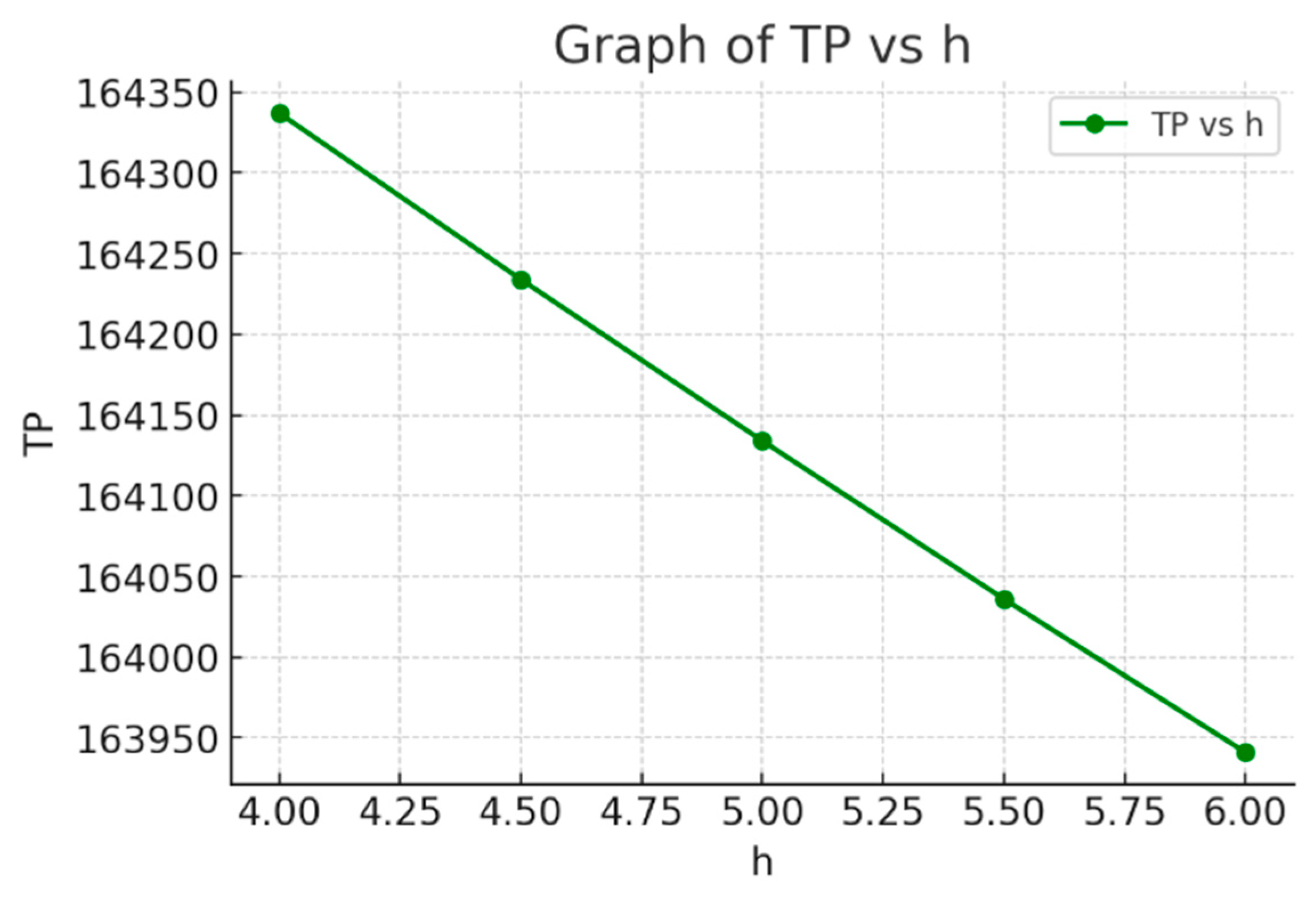
| (Yr) | E[TPU] ($) | |
|---|---|---|
| 6.0 | 0.053319 | 163941 |
| 5.5 | 0.054671 | 164036 |
| 5.0 | 0.056133 | 164134 |
| 4.5 | 0.057718 | 164234 |
| 4.0 | 0.059447 | 164337 |
| (Yr) | E[TPU] ($) | |
|---|---|---|
| 0.02 | 0.056197 | 164135 |
| 0.04 | 0.056165 | 164134 |
| 0.06 | 0.056133 | 164134 |
| 0.08 | 0.056100 | 164133 |
| 0.10 | 0.056068 | 164132 |
Disclaimer/Publisher’s Note: The statements, opinions and data contained in all publications are solely those of the individual author(s) and contributor(s) and not of MDPI and/or the editor(s). MDPI and/or the editor(s) disclaim responsibility for any injury to people or property resulting from any ideas, methods, instructions or products referred to in the content. |
© 2025 by the authors. Licensee MDPI, Basel, Switzerland. This article is an open access article distributed under the terms and conditions of the Creative Commons Attribution (CC BY) license (https://creativecommons.org/licenses/by/4.0/).
Share and Cite
Bansal, A.; Panwar, A.; Unhelkar, B.; Mittal, M. Optimizing Inventory for Imperfect and Gradually Deteriorating Items Under Multi-Level Trade Credit in a Sustainable Supply Chain. Mathematics 2025, 13, 752. https://doi.org/10.3390/math13050752
Bansal A, Panwar A, Unhelkar B, Mittal M. Optimizing Inventory for Imperfect and Gradually Deteriorating Items Under Multi-Level Trade Credit in a Sustainable Supply Chain. Mathematics. 2025; 13(5):752. https://doi.org/10.3390/math13050752
Chicago/Turabian StyleBansal, Abhay, Aastha Panwar, Bhuvan Unhelkar, and Mandeep Mittal. 2025. "Optimizing Inventory for Imperfect and Gradually Deteriorating Items Under Multi-Level Trade Credit in a Sustainable Supply Chain" Mathematics 13, no. 5: 752. https://doi.org/10.3390/math13050752
APA StyleBansal, A., Panwar, A., Unhelkar, B., & Mittal, M. (2025). Optimizing Inventory for Imperfect and Gradually Deteriorating Items Under Multi-Level Trade Credit in a Sustainable Supply Chain. Mathematics, 13(5), 752. https://doi.org/10.3390/math13050752