

Use Cases of Machine Learning in Queueing Theory Based on a GI/G/K System


Abstract
1. Introduction
2. Related Publications
3. Main Model and Data Generation
4. Simulation Techniques
4.1. Event-Based Simulation
| Algorithm 1 Event-based simulation | |
Require: , , , ,
|
4.2. Simulation by Moments of Departure
| Algorithm 2 Simulation by moments of departure |
Require: ,
|
4.3. Validation of the Simulation Model
- 1.
- Initialize the system parameters , where the PH distributions for the arrival stream of customers and for their service times are given by two transient states and are represented asThe probabilities are chosen randomly from the interval , and the intensities and from the interval . A data set of parameter values and with the length 125 satisfying the condition is generated. Here, we deliberately exclude cases of heavy traffic, when the data obtained with the simulator have the highest variance.
- 2.
- We calculate the mathematical expectation and the square of the coefficient of variation of the corresponding random variables using Formula (2),For b and , we obtain similar relations by replacing by and by .
- 3.
- Initialization of parameters of other time distributions of T is performed depending on the moments defined above. For the gamma distribution () with parameters and density functionthe parameters are calculated from the relationsFor a Pareto distribution () with parameters and density functionthe parameters depend on the moments of the random variable T in accordance with the relationsFinally, for a lognormal distribution () with parameters and density functionthe parameters are defined as
- 4.
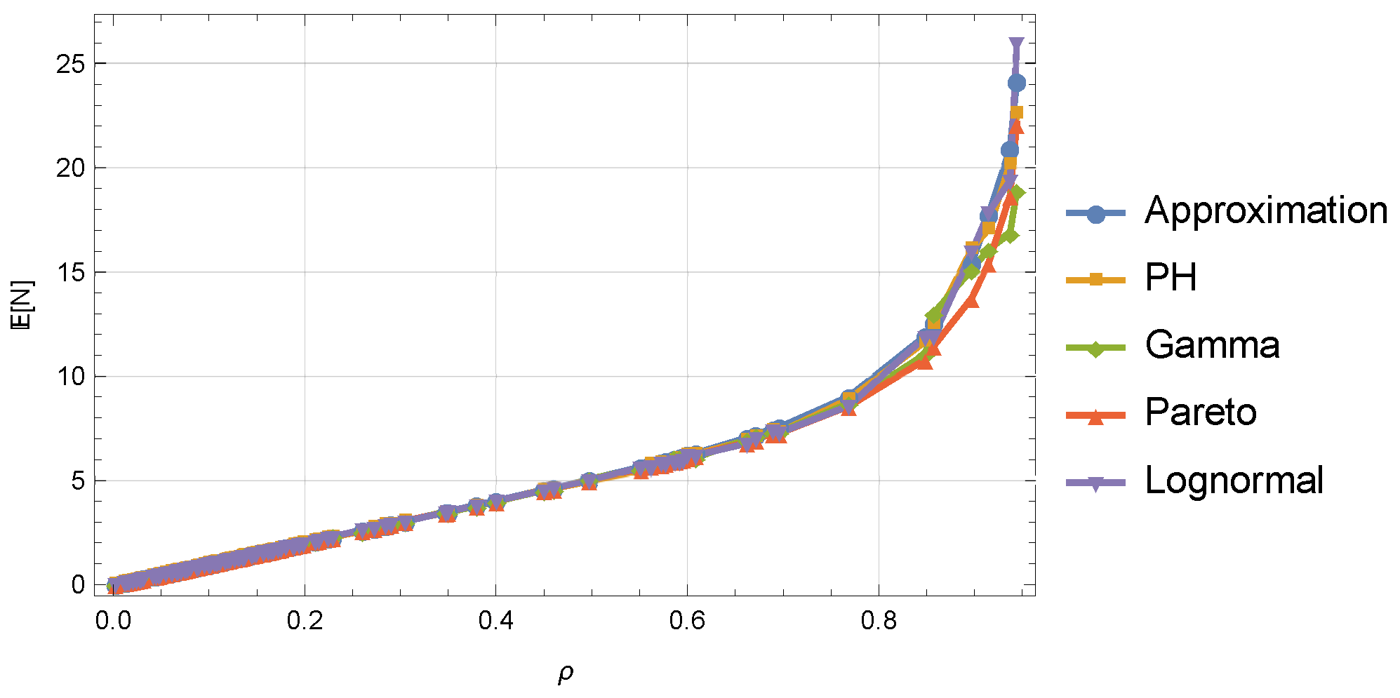
- We calculate the average number of customers in the system using the approximation (3) and the simulation models proposed above for systems , , , . Here, in principle, any combination of distributions could be used. We illustrate the computational results in form of pairs in Figure 2. The evaluation of the load factor of the system is based on the values of parameters for arrival and service processes generated in step 1. As we can see, the curves match to a large extent. Some deviations are observed as the system load increases, e.g., for , especially for the Pareto distribution. This is due to the increase in the variance of the estimate of the average number of customers in the system at higher loads. In addition, the Pareto distribution has heavy tails, due to which the system can be characterized by slower growth of the number of customers in the system at the same load compared to other distributions. Thus, the choice of the first two moments of the interarrival and the the service times as characteristic features for estimating the average metrics of the given queueing system is quite justified.
- 5.
- The final part in the validation process of the simulation models is the comparison of the two algorithms, discrete-event and by the departure moments, with the exact values obtained for the queueing system. Figure 3 shows the results of calculations of the average number of customers in the system depending on the load factor using simulation models and explicit formulaAs we can see, the graphs are indistinguishable up to a certain value of , and, only at high load, small deviations are observed due to the large variance of the obtained estimates. When simulating queues in heavy traffic, estimators of mean characteristics converge slowly to their true values. This problem is exacerbated when the distributions of interarrival and service times have heavy tails.
5. Regression Tasks
5.1. Estimation of the Average Number of Customers in the System
5.2. Estimation of the Distribution for the Number of Customers in the System
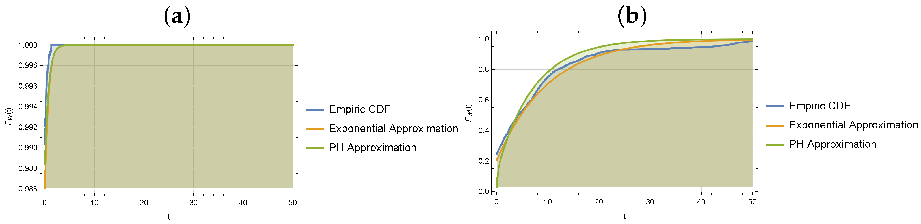
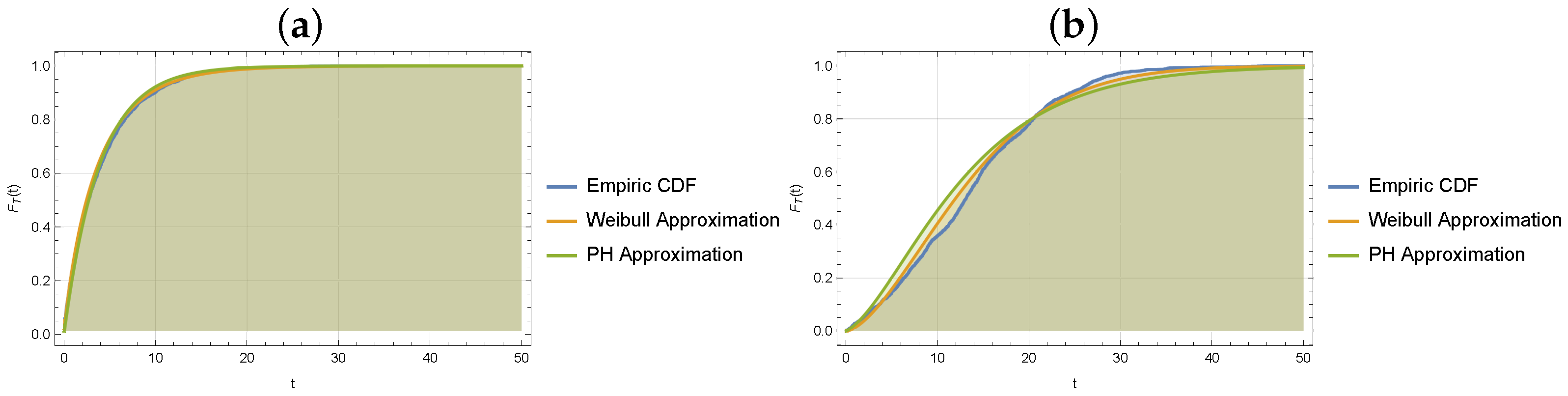
5.3. Estimation of the Waiting and Sojourn Time Distributions
6. Classification Tasks
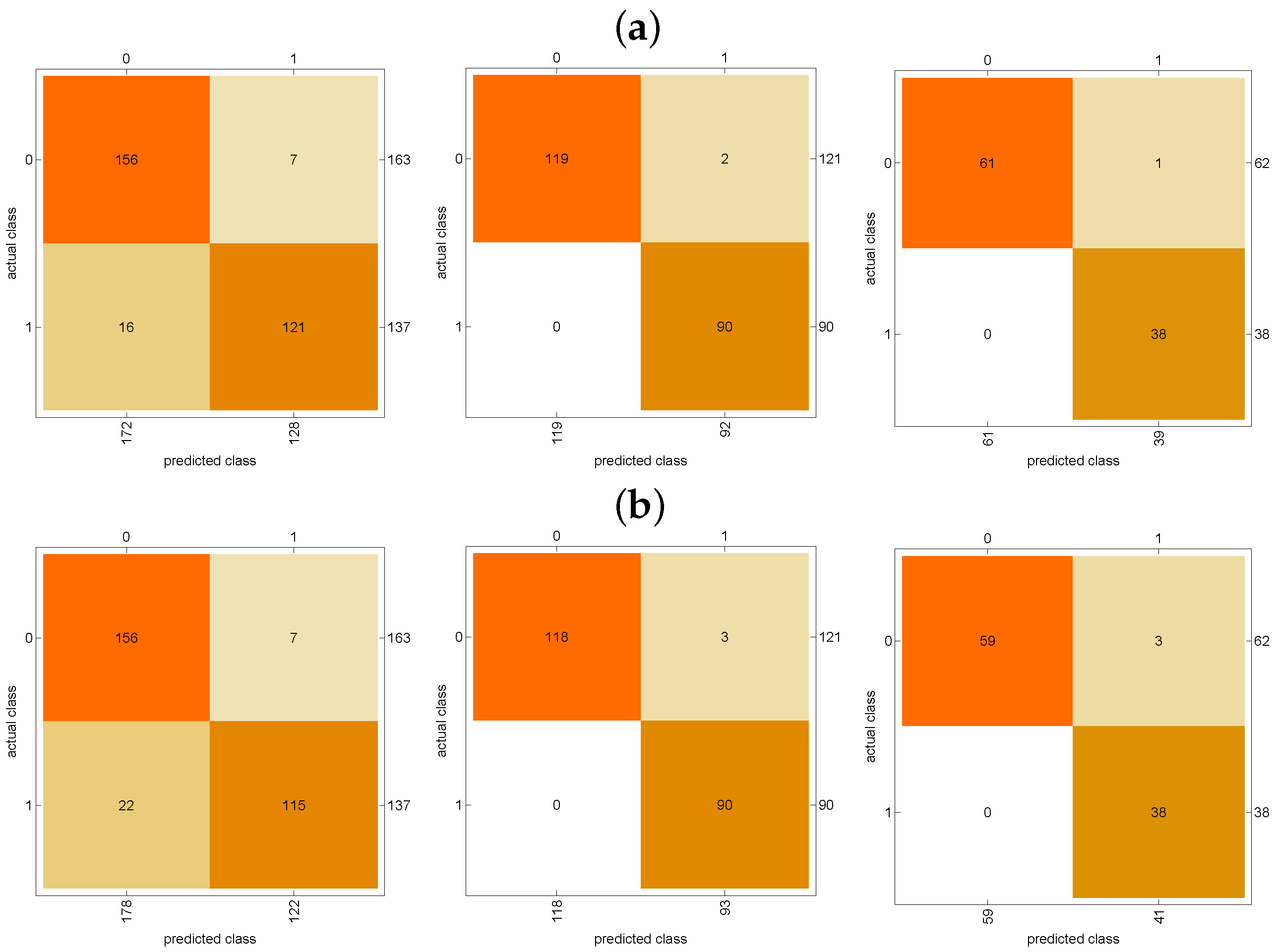
6.1. Classifying by Waiting Time Threshold
6.2. Classification in Parametric Optimization Problem
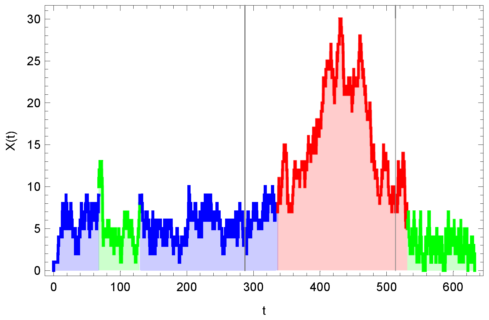
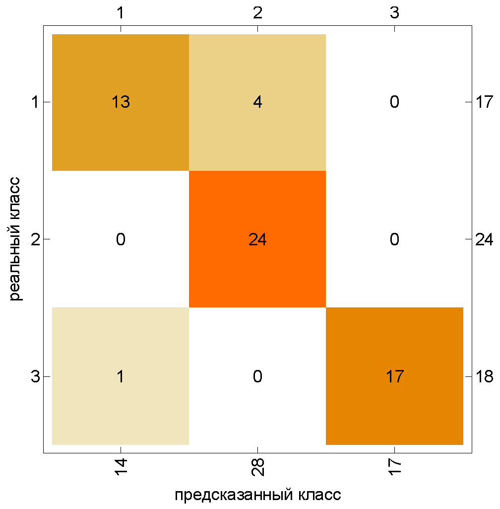
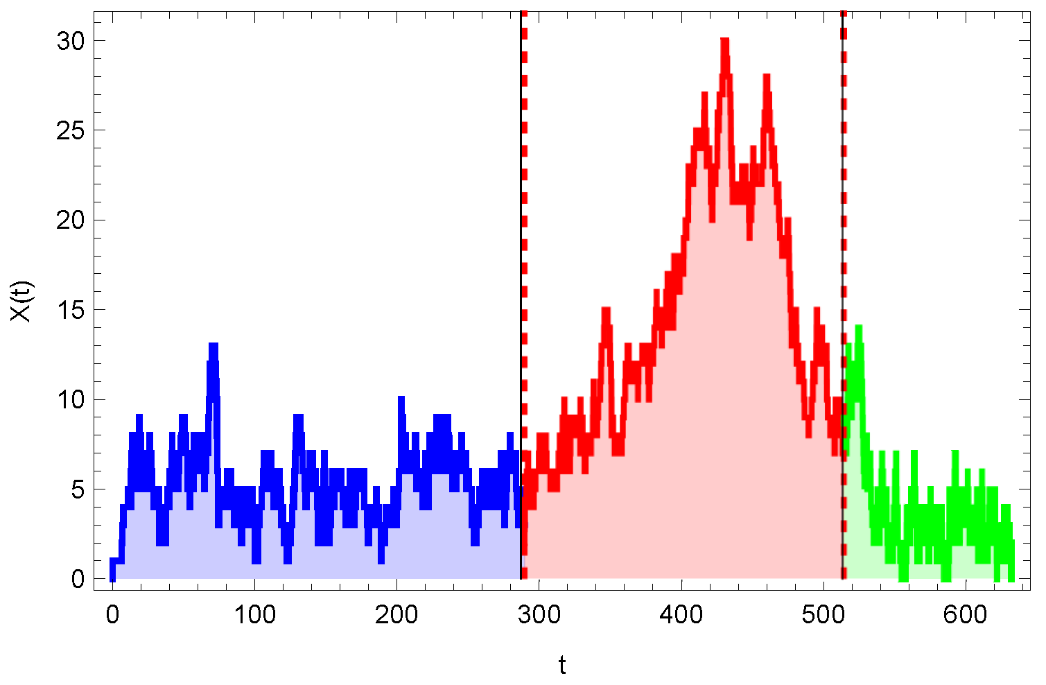
6.3. Classification of Queueing Systems by Time Series
- Class 1: ,, , , .
- Class 2:, , , .
- Class 3:, , , .
- —system load factor, estimated as the average number of occupied servers, i.e., ;
- —arrival rate, estimated as the number of incoming customers per unit of a given time interval;
- —rate of change of the number of customers in the system at the corresponding time interval;
- —length of the partial series interval containing 20 events.
7. Reinforcement Learning for Dynamic Optimization
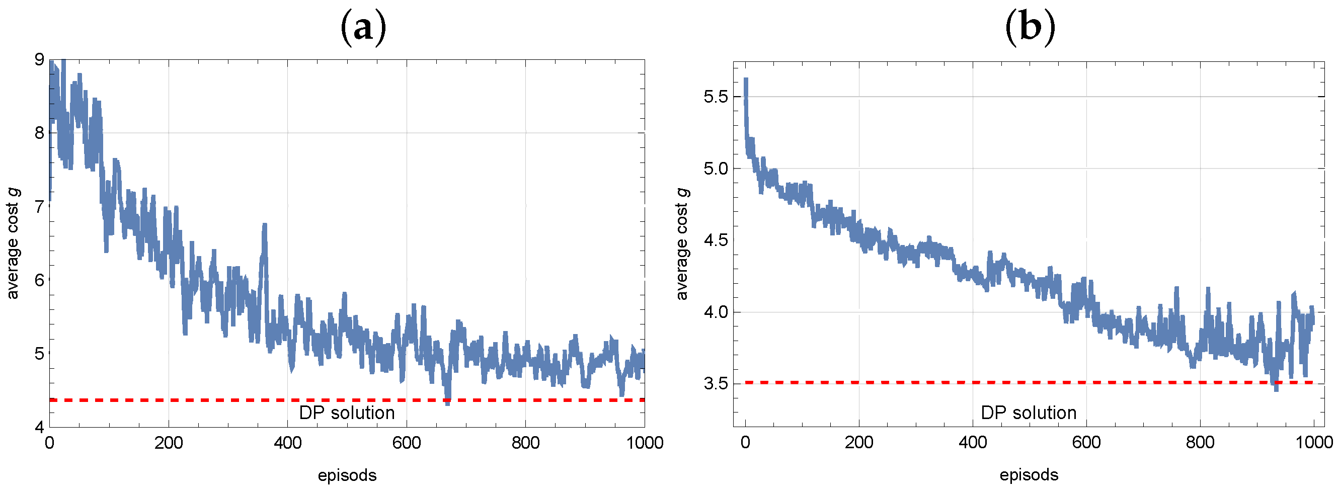
7.1. DP Approach
- Case 1: , , for ,
- Case 2: , , for .
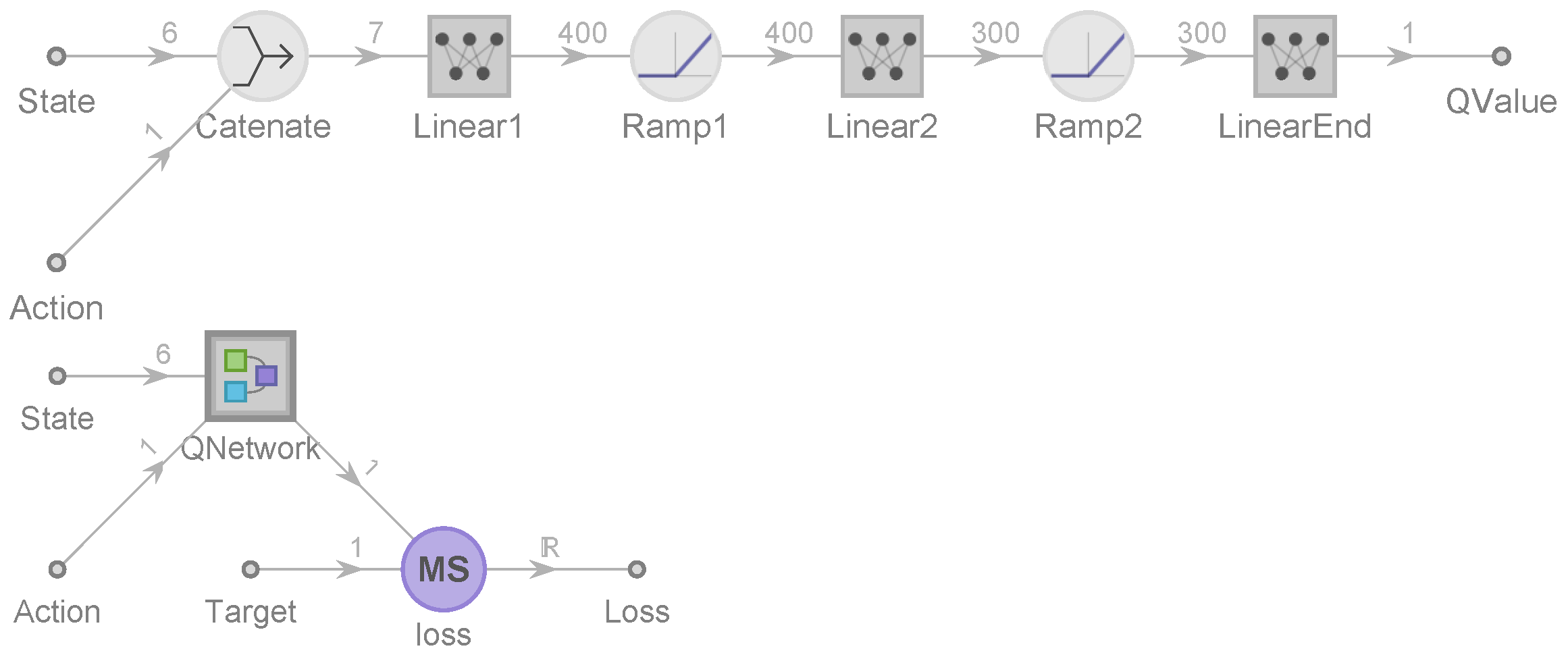
7.2. RL Approach
- 1.
- Initialization. Initialize quality function , , , , , which counts the times of occurrence of the state x.
- 2.
- Policy evaluation. While Q-values are not converged, perform the following steps.
- 3.
- Evaluation and update of the sample Q. . Forupdate the values of Q with respect to (16) with a learning rate .
- 4.
- Policy improvement. Q to conversion. After a convergence in one episode, a new policy is generated using the relation . Then setfor all .
- 1.
- Initialization. Initialize the policy network with random weights W, initialize D. For to K, perform the following steps.
- 2.
- .
- 3.
- Calculate the target Q-value
- 4.
- Calculate the loss between predicted and target Q-values
- 5.
- Back propagate the loss and update the weights .
- 6.
- Periodically update .
8. Conclusions
Author Contributions
Funding
Data Availability Statement
Conflicts of Interest
References
- Oladipupo, T. Types of Machine Learning Algorithms. In New Advances in Machine Learning; InTech: Rijeka, Croatia, 2010; Chapter 3. [Google Scholar] [CrossRef]
- Hastie, T.; Tibshirani, R.; Friedman, J. The Elements of Statistical Learning; Springer: New York, NY, USA, 2009. [Google Scholar] [CrossRef]
- Bishop, C.M. Pattern Recognition and Machine Learning (Information Science and Statistics); Springer: Berlin/Heidelberg, Germany, 2006. [Google Scholar]
- Sutton, R.; Barto, A. Reinforcement Learning: An Introduction. IEEE Trans. Neural Netw. 1998, 9, 1054. [Google Scholar] [CrossRef]
- Choi, D.; Kim, N.; Chae, K. A Two-Moment Approximation for the GI/G/c Queue with Finite Capacity. INFORMS J. Comput. 2005, 17, 75–81. [Google Scholar] [CrossRef]
- Shore, H. Simple Approximations for the GI/G/c Queue-I: The Steady-State Probabilities. J. Oper. Res. Soc. 1988, 39, 279. [Google Scholar] [CrossRef]
- Shore, H. Simple Approximations for the GI/G/c Queue-II: The Moments, the Inverse Distribution Function and the Loss Function of the Number in the System and of the Queue Delay. J. Oper. Res. Soc. 1988, 39, 381–391. [Google Scholar] [CrossRef]
- Shortle, J.; Thompson, J.; Gross, D.; Harris, C. Fundamentals of Queueing Theory; Wiley: Hoboken, NJ, USA, 2018. [Google Scholar] [CrossRef]
- Van Hoorn, M.; Seelen, L. Approximations for the GI/G/c queue. J. Appl. Probab. 1986, 23, 484–494. [Google Scholar] [CrossRef]
- Whitt, W. The Queueing Network Analyzer. Bell Syst. Tech. J. 1983, 62, 2779–2815. [Google Scholar] [CrossRef]
- Shin, Y.; Moon, D. On approximations for GI/G/c retrial queues. J. Appl. Math. Inform. 2013, 31, 311–325. [Google Scholar] [CrossRef]
- Telek, M.; Heindl, A. Matching Moments For Acyclic Discrete And Continuous Phase-Type Distributions Of Second Order. Int. J. Simul. Syst. Sci. Technol. 2003, 3, 47–57. [Google Scholar]
- Vishnevsky, V.; Gorbunova, A.V. Application of Machine Learning Methods to Solving Problems of Queuing Theory. In Information Technologies and Mathematical Modelling. Queueing Theory and Applications; Springer International Publishing: Cham, Switzerland, 2022; pp. 304–316. [Google Scholar] [CrossRef]
- Stintzing, J.; Norrman, F. Prediction of queuing behaviour through the use of artificial neural networks. In Proceedings of the Computer Science. 2017. Available online: https://api.semanticscholar.org/CorpusID:198923796 (accessed on 3 February 2025).
- Nii, S.; Okudal, T.; Wakita, T. A Performance Evaluation of Queueing Systems by Machine Learning. In Proceedings of the 2020 IEEE International Conference on Consumer Electronics—Taiwan (ICCE-Taiwan), Taoyuan, Taiwan, 28–30 September 2020; IEEE: Piscataway, NJ, USA, 2020. [Google Scholar] [CrossRef]
- Sherzer, E.; Senderovich, A.; Baron, O.; Krass, D. Can machines solve general queueing systems? arXiv 2022. [CrossRef]
- Kyritsis, A.I.; Deriaz, M. A Machine Learning Approach to Waiting Time Prediction in Queueing Scenarios. In Proceedings of the 2019 Second International Conference on Artificial Intelligence for Industries (AI4I), Laguna Hills, CA, USA, 25–27 September 2019; IEEE: Piscataway, NJ, USA, 2019. [Google Scholar] [CrossRef]
- Sivakami, S.; Senthil, K.; Yamini, S.; Palaniammal, S. Artificial neural network simulation for markovian queueing models. Indian J. Comput. Sci. Eng. 2020, 11, 127–134. [Google Scholar] [CrossRef]
- Hijry, H.; Olawoyin, R. Predicting Patient Waiting Time in the Queue System Using Deep Learning Algorithms in the Emergency Room. Int. J. Ind. Eng. Oper. Manag. 2021, 3, 33–45. [Google Scholar] [CrossRef]
- Chocron, E.; Cohen, I.; Feigin, P. Delay Prediction for Managing Multiclass Service Systems: An Investigation of Queueing Theory and Machine Learning Approaches. IEEE Trans. Eng. Manag. 2022, 71, 4469–4479. [Google Scholar] [CrossRef]
- Dieleman, N.; Berkhout, J.; Heidergott, B. A neural network approach to performance analysis of tandem lines: The value of analytical knowledge. Comput. Oper. Res. 2023, 152, 106124. [Google Scholar] [CrossRef]
- Vishnevsky, V.; Klimenok, V.; Sokolov, A.; Larionov, A. Performance Evaluation of the Priority Multi-Server System MMAP/PH/M/N Using Machine Learning Methods. Mathematics 2021, 9, 3236. [Google Scholar] [CrossRef]
- Klimenok, V.; Dudin, A.; Vishnevsky, V. Priority multi-server queueing system with heterogeneous customers. Mathematics 2020, 8, 1501. [Google Scholar] [CrossRef]
- Vishnevsky, V.; Larionov, A.; Mukhtarov, A.; Sokolov, A. Investigation of Tandem Queuing Systems Using Machine Learning Methods. Control Probl. 2024, 4, 13–25. [Google Scholar] [CrossRef]
- Vishnevsky, V.; Larionov, A.; Semenova, O.; Ivanov, R. State Reduction in Analysis of a Tandem Queueing System with Correlated Arrivals. In Information Technologies and Mathematical Modelling. Queueing Theory and Applications; Dudin, A., Nazarov, A., Kirpichnikov, A., Eds.; Springer: Cham, Switzerland, 2017; pp. 215–230. [Google Scholar]
- Klimenok, V.; Dudina, O.; Vishnevsky, V.; Samouylov, K. Retrial Tandem Queue with BMAP-Input and Semi-Markovian Service Process. In Distributed Computer and Communication Networks; Vishnevskiy, V., Samouylov, K., Kozyrev, D., Eds.; Springer International Publishing: Cham, Switzerland, 2017; pp. 159–173. [Google Scholar]
- Vishnevsky, V.; Semenova, O.; Bui, D. Using a Machine Learning Approach for Analysis of Polling Systems with Correlated Arrivals. In Distributed Computer and Communication Networks: Control, Computation, Communications; Springer International Publishing: Cham, Switzerland, 2021; pp. 336–345. [Google Scholar] [CrossRef]
- Vishnevsky, V.; Semenova, O. Polling Systems and Their Application to Telecommunication Networks. Mathematics 2021, 9, 117. [Google Scholar] [CrossRef]
- Efrosinin, D.; Vishnevsky, V.; Stepanova, N. A Machine-Learning Approach To Queue Length Estimation Using Tagged Customers Emission. In Distributed Computer and Communication Networks: Control, Computation, Communications 2023; Springer International Publishing: Cham, Switzerland, 2024; pp. 265–276. [Google Scholar] [CrossRef]
- Vishnevsky, V.; Klimenok, V.; Sokolov, A.; Larionov, A. Investigation of the Fork–Join System with Markovian Arrival Process Arrivals and Phase-Type Service Time Distribution Using Machine Learning Methods. Mathematics 2024, 12, 659. [Google Scholar] [CrossRef]
- Ivanova, N.; Vishnevsky, V. Application of k-out-of-n:G System and Machine Learning Techniques on Reliability Analysis of Tethered Unmanned Aerial Vehicle. In Proceedings of the Information Technologies and Mathematical Modelling. Queueing Theory and Applications; Dudin, A., Nazarov, A., Moiseev, A., Eds.; Springer: Cham, Switzerland, 2022; Volume 1605, pp. 117–130. [Google Scholar]
- Alfa, A.S.; Abu Ghazaleh, H. Machine Learning Tool for Analyzing Finite Buffer Queueing Systems. Mathematics 2025, 13, 346. [Google Scholar] [CrossRef]
- Matsumoto, Y. On optimization of polling policy represented by neural network. ACM SIGCOMM Comput. Commun. Rev. 1994, 24, 181–190. [Google Scholar] [CrossRef]
- Kohonen, T. The self-organizing map. Proc. IEEE 1990, 78, 1464–1480. [Google Scholar] [CrossRef]
- Efrosinin, D.; Rykov, V.; Stepanova, N. Evaluation and Prediction of an Optimal Control in a Processor Sharing Queueing System with Heterogeneous Servers. In Distributed Computer and Communication Networks; Springer International Publishing: Cham, Switzerland, 2020; pp. 450–462. [Google Scholar] [CrossRef]
- Efrosinin, D.; Vishnevsky, V.; Stepanova, N. Optimal Scheduling in General Multi-Queue System by Combining Simulation and Neural Network Techniques. Sensors 2023, 23, 5479. [Google Scholar] [CrossRef]
- Li, Q.L.; Ma, J.Y.; Fan, R.N.; Xia, L. An Overview for Markov Decision Processes in Queues and Networks. arXiv 2019. [Google Scholar] [CrossRef]
- Özkan, E.; Kharoufeh, J.P. Optimal control of a two-server queueing system with failures. Probab. Eng. Inf. Sci. 2014, 28, 489–527. [Google Scholar] [CrossRef]
- Watkins, C.J.C.H.; Dayan, P. Q-learning. Mach. Learn. 1992, 8, 279–292. [Google Scholar] [CrossRef]
- Li, Y. Deep Reinforcement Learning: An Overview. arXiv 2017. [Google Scholar] [CrossRef]
- Van Hasselt, H.; Guez, A.; Silver, D. Deep Reinforcement Learning with Double Q-Learning. In Proceedings of the AAAI Conference on Artificial Intelligence, Phoenix, AZ, USA, 12–17 February 2016; Volume 30. [Google Scholar] [CrossRef]
- Thomas, P.S.; Brunskill, E. Policy Gradient Methods for Reinforcement Learning with Function Approximation and Action-Dependent Baselines. arXiv 2017. [Google Scholar] [CrossRef]
- Konda, V.; Tsitsiklis, J. Actor-Critic Algorithms. In Proceedings of the Advances in Neural Information Processing Systems; Solla, S., Leen, T., Müller, K., Eds.; MIT Press: Cambridge, MA, USA, 1999; Volume 12. [Google Scholar]
- Lillicrap, T.P.; Hunt, J.J.; Pritzel, A.; Heess, N.; Erez, T.; Tassa, Y.; Silver, D.; Wierstra, D. Continuous control with deep reinforcement learning. arXiv 2015. [Google Scholar] [CrossRef]
- Okumu, E.M. A deep reinforcement learning approach to queue management and revenue maximization in multi-tier 5G wireless networks. Am. Acad. Sci. Res. J. Eng. Technol. Sci. (ASRJETS) 2021, 84, 15–26. [Google Scholar]
- Jali, N.; Qu, G.; Wang, W.; Joshi, G. Efficient Reinforcement Learning for Routing Jobs in Heterogeneous Queueing Systems. arXiv 2024. [Google Scholar] [CrossRef]
- Efrosinin, D.; Vishnevsky, V.; Stepanova, N. Simulation-Based Optimization for Resource Allocation Problem in Finite-Source Queue with Heterogeneous Repair Facility. In Distributed Computer and Communication Networks; Vishnevsky, V.M., Samouylov, K.E., Kozyrev, D.V., Eds.; Springer: Cham, Switzerland, 2025; pp. 187–202. [Google Scholar]
- Rebuffi, L.S. Reinforcement Learning Algorithms for Controlled Queueing Systems. Ph.D. Thesis, University of Grenoble Alpes, Grenoble, France, 2014. [Google Scholar]
- Asmussen, S. Applied Probability and Queues; Springer: New York, NY, USA, 2003. [Google Scholar] [CrossRef]
- Bolch, G.; Greiner, S.; de Meer, H.; Trivedi, K.S. Steady-State Solutions of Markov Chains; Wiley: Hoboken, NJ, USA, 1998. [Google Scholar] [CrossRef]
- Cox, D. A use of complex probabilities in the theory of stochastic processes. Math. Proc. Camb. Philos. Soc. 1955, 51, 313–319. [Google Scholar] [CrossRef]
- Choudhury, A. A Simple Derivation of Moments of the Exponentiated Weibull Distribution. Metrika 2005, 62, 17–22. [Google Scholar] [CrossRef]
- Younes, H.L.S.; Simmons, R.G. Solving Generalized Semi-Markov Decision Processes Using Continuous Phase-Type Distributions. In Proceedings of the Nineteenth National Conference on Artificial Intelligence, Sixteenth Conference on Innovative Applications of Artificial Intelligence, San Jose, CA, USA, 25–29 July 2004; McGuinness, D.L., Ferguson, G., Eds.; AAAI Press/The MIT Press: Cambridge, MA, USA, 2004; pp. 742–748. [Google Scholar]


| (a) | (b) | ||||
|---|---|---|---|---|---|
| Method | Method | ||||
| Nearest Neighbors | 0.147 | 0.990 | Nearest Neighbors | 5.860 | 0.765 |
| Decision Tree | 0.111 | 0.994 | Decision Tree | 6.020 | 0.751 |
| Random Forest | 0.447 | 0.903 | Random Forest | 5.770 | 0.772 |
| Gradient Boosted Tree | 0.253 | 0.969 | Gradient Boosted Tree | 5.690 | 0.778 |
| Gauss Regression. | 0.443 | 0.909 | Gauss Regression | 5.650 | 0.781 |
| Neural Network | 0.088 | 0.996 | Neural Network | 5.780 | 0.771 |
| Arrival | |||||
|---|---|---|---|---|---|
| Service | |||||
| Method | Threshold w | Accuracy | Entropy |
|---|---|---|---|
| Logistic Regression | 0 | 0.923 | 0.193 |
| Neural Network | 0 | 0.903 | 0.215 |
| Logistic Regression | 4 | 0.991 | 0.034 |
| Neural Network | 4 | 0.927 | 0.076 |
| Logistic Regression | 7 | 0.990 | 0.101 |
| Neural Network | 7 | 0.970 | 0.099 |
| Methods | Accuracy | Entropy |
|---|---|---|
| Logistic Regression | 0.857 | 0.323 |
| Nearest Neighbor | 0.847 | 0.367 |
| Decision Tree | 0.880 | 0.339 |
| Random Forest | 0.895 | 0.300 |
| Gradient Boosted Tree | 0.898 | 0.255 |
| Support Vector Machine | 0.788 | 0.506 |
| Naive Bayes | 0.857 | 0.387 |
| Markov Model | 0.698 | 0.824 |
| Neural Network | 0.887 | 0.351 |
| Method | Accuracy | Entropy |
|---|---|---|
| Logistic Regression | 0.612 | 0.865 |
| Nearest Neighbor | 0.847 | 0.465 |
| Decision Tree | 0.817 | 0.566 |
| Random Forest | 0.845 | 0.393 |
| Gradient Boosted Tree | 0.840 | 0.484 |
| Support Vector Machine | 0.716 | 0.810 |
| Naive Bayes | 0.668 | 0.760 |
| Markov Model | 0.527 | 3.350 |
| Neural Network | 0.742 | 0.548 |
Disclaimer/Publisher’s Note: The statements, opinions and data contained in all publications are solely those of the individual author(s) and contributor(s) and not of MDPI and/or the editor(s). MDPI and/or the editor(s) disclaim responsibility for any injury to people or property resulting from any ideas, methods, instructions or products referred to in the content. |
© 2025 by the authors. Licensee MDPI, Basel, Switzerland. This article is an open access article distributed under the terms and conditions of the Creative Commons Attribution (CC BY) license (https://creativecommons.org/licenses/by/4.0/).
Share and Cite
Efrosinin, D.; Vishnevsky, V.; Stepanova, N.; Sztrik, J. Use Cases of Machine Learning in Queueing Theory Based on a GI/G/K System. Mathematics 2025, 13, 776. https://doi.org/10.3390/math13050776
Efrosinin D, Vishnevsky V, Stepanova N, Sztrik J. Use Cases of Machine Learning in Queueing Theory Based on a GI/G/K System. Mathematics. 2025; 13(5):776. https://doi.org/10.3390/math13050776
Chicago/Turabian StyleEfrosinin, Dmitry, Vladimir Vishnevsky, Natalia Stepanova, and Janos Sztrik. 2025. "Use Cases of Machine Learning in Queueing Theory Based on a GI/G/K System" Mathematics 13, no. 5: 776. https://doi.org/10.3390/math13050776
APA StyleEfrosinin, D., Vishnevsky, V., Stepanova, N., & Sztrik, J. (2025). Use Cases of Machine Learning in Queueing Theory Based on a GI/G/K System. Mathematics, 13(5), 776. https://doi.org/10.3390/math13050776