Abstract
Let denote the second symmetric product of the complex plane endowed with the Hausdorff topology, i.e., . In this paper, we extended the concept of Möbius transformations to . More precisely, given a Möbius transformation T of , we define the map within . We describe some general properties of these maps, including the structure of their generators, characteristics related to transitivity, and the geometry of the conjugacy classes.
MSC:
30G35; 54H15
1. Introduction
The second symmetric product of the complex plane is defined as the set ; that is, consists of points of the form , with and , and points of the form , called singletons when , endowed with the Hausdorff metric (see [1,2,3] for more about symmetric products of topological spaces). In this paper, we translated the properties of the Möbius transformations of the Riemann sphere to the space .
Consider a Möbius transformation , where denotes the one-point compactification of , i.e., is the Riemann sphere. We extend the notion of Möbius transformation to as follows. Given a point , we define as , whenever T is defined in z and w; note that , if .
The purpose of this paper is to extend the study of the geometry of the Möbius transformations in the second symmetric product of the complex plane . To do that, we introduced a model for . That is, there is a homeomorphism from to a more suitable space in which we can have a better understanding of the geometry induced by . The homeomorphic model of is the space
where and s is a relation on elements of the form ; see Section 2.3 below.
Given , a Möbius transformation in the Riemann sphere, recall that for , , so we need to change the definition of when z or w is equal to ; this change will produce discontinuities at some points, but on the other hand, the change will be compatible with having some results similar to properties inherent in the set of Möbius transformations.
We start with the basic results of the classical theory of Möbius transformations in Section 2. In addition, we describe the topology of the second symmetric product of and the model for .
In Section 3, we define the set , where each is taken with its corresponding domain and image, and Aut is the set of complex automorphisms of , that is, the set of all automorphisms of the Riemann sphere; see Section 2.1. That is, we properly defined the extension of a Möbius transformation to the space . We look closely at how the domains of these maps change depending on T; for instance, we describe the maximum domain where any map is continuous, for any Möbius transformation T. We also describe the action of these maps , via the extension to of the usual generators of the group of Möbius transformations; that is, we prove in Proposition 1 that any map in is a composition of the extensions to of the maps described in Theorem 1. We study in Propositions 2–5 the action of the generators of in the space .
Some transitivity properties of the usual Möbius transformations can be translated on transitivity features of the set in , which we described in Section 4. In Proposition 8, we prove that is 2-transitive in if the corresponding points have the same cross ratio.
Now, considering the set of Euclidean circles and the family of lines in , the corresponding objects in are Möbius strips and semi-planes, respectively. Proving first that sends the set of these Möbius strips and semi-planes into itself, we show in Theorem 9 that acts transitively in this set. We also define maps that preserve the Möbius strips in generated by Euclidean circles in . These maps are the extensions to of inversions in Euclidean circles in the Riemann sphere, and we finish Section 4 proving some properties for these maps.
As any Möbius transformation T, different from the identity, is conjugated to a map of the form with or to the map , in Section 5, we extend this result for maps in the set in Theorems 11–13, depending on whether T is parabolic, hyperbolic, or elliptic, respectively. Finally, we show how the corresponding maps act in .
In summary, in this paper, we explain how the classical theory of Möbius transformations in the Riemann sphere can be extended not just to or but to different topological spaces, as we have done in the second symmetric product of the complex plane. This extension includes the description of the generators of and how they behave geometrically in the model , which allows us to observe some similarities with the geometry of the orbits of points under classical Möbius transformations. We also prove that has some transitivity properties; for instance, we prove transitivity in a large set of Möbius strips contained in , and they are characterized using cross ratio; moreover, we prove that the concept of inversion in a Euclidean circle can be extended to an inversion in a Möbius strip. Finally, we extend the geometric classification of conjugacy classes in Aut to our setting, describing geometrically the representatives of every conjugacy class.
We would like to note that extending the Möbius transformations to the second symmetric space allows us to explore this space from the perspective of conformal geometry. This approach makes even more intriguing, as it retains all the properties we have proven.
Furthermore, we highlight that in recent years, several open problems in plane geometry have been resolved by examining the non-embeddability of the second symmetric product of certain spaces into and (see [4,5,6]). In light of these findings, we believe it is crucial to study, in general, the second symmetric product of . We consider it possible that certain geometric problems in the plane can be translated to different geometric spaces, as it is demonstrated by the results mentioned above.
2. Preliminaries
In this section, we will briefly present the definitions and results of Möbius transformations and the second symmetric product of , which we will need in the rest of the paper.
2.1. Möbius Transformations
First, let us describe some basic facts, properties, and results about Möbius transformations in the Riemann sphere; for more details, see [7,8], where all the definitions and proofs of the results stated here can be found. Let be the Riemann sphere. We will denote by Aut the set of all automorphisms of , that is, functions of the form
with complex numbers such that . Transformations are known as linear fractional or Möbius transformations. These transformations form a group under composition, where the inverse map of T is given by
There is a group homomorphism from the group of matrices of 2 by 2 with complex coefficients, , to the group Aut; its kernel is the set K of all matrices of the form , (), where I is the identity matrix. Hence, Aut is isomorphic to the group , the projective general linear group.
Equivalently, as T does not determine the coefficients uniquely, since , , , correspond to the same transformation T, for , we see again that the group Aut is isomorphic to the projective general linear group. It can be proven that Aut is also isomorphic to the projective special linear group, that is, the group , where each element has determinant equal to 1; see Theorem 2.1.3 in [7], which states that Aut. Thus, from now on, we can assume that .
The group Aut is generated by four special types of Möbius transformations, as is stated in the following theorem.
Theorem 1.
Any element in Aut can be written as a composition of maps of the following form:
- (i)
- The map ( is a rotation of the Riemann sphere by an angle θ.
- (ii)
- The transformation , that interchange zero and ∞.
- (iii)
- The map () fixes 0 and ∞, and acts in the plane as a similarity transformation.
- (iv)
- The transformation () fixes ∞ and acts as a translation in the complex plane.
One important property of the automorphisms of is that they send circles in to circles in . To be more precise, the circles in are the usual Euclidean circles, and the straight lines in (which can be thought of as circles through infinity).
Theorem 2.
If C is a circle in and Aut, then is a circle in .
The group Aut also has several properties about transitivity; the following are the ones we will use in this paper.
Theorem 3.
If and are triples of distinct points in , then there is a unique Aut such that , for .
Corollary 1.
If Aut and T fixes three distinct points of , then T is the identity map.
Theorem 4.
If C and are circles in , then there exists some Aut such that .
In general, Aut is not 4-transitive, but if two 4-tuple of distinct points have the same cross-ratio, there is some Möbius transformation that sends one 4-tuple into the other. Recall that the cross-ratio of four complex numbers is defined as with the convention of taking limits if some .
Theorem 5.
Let and be 4-tuples of distinct elements of . Then, there exists some Aut with , if and only if the two 4-tuples have the same cross-ratio.
Consider a circle C in given by the equation , with , . If , then C is an Euclidean circle in the complex plane, and then a transformation exists in the complex plane that fixes C. This transformation is given by
which is called the inversion in C. Moreover, if Aut, then is another circle, and we have that .
To study the geometry of the Möbius transformations, we would like to recall that there is a classification of the automorphisms of in conjugacy classes, according to the number of fixed points, and the corresponding trace of the matrix associated in . The next results summarize this classification.
Theorem 6.
Let , with . If , then T has two fixed points in ; if and T is not the identity map, T has one fixed point in .
For , consider the maps if and . We will say that two maps T and S are conjugated if there exists another transformation V such that .
Theorem 7.
Let T be a non-identity element in Aut; then, there exists some such that T is conjugate to in Aut.
Remark 1.
When , the map T has only one fixed point , and it is conjugated to by a Möbius transformation S that sends to ∞. Since , any is moved by towards as n goes to infinity. In this case, T is called parabolic.
Remark 2.
If T is not parabolic, then it has two fixed points and and is conjugated to , with , that fixes 0 and ∞, by means of a Möbius transformation S such that and . If , for all and hence for all . In the same way, if , then for all (the two cases for λ are the same since we can replace λ by ). We conclude that if , all points are moved by T away from one of these fixed points towards the other. If , T is called hyperbolic and loxodromic otherwise. If , with , then is a rotation , so has no limit for ; hence neither for . In this case, T is called elliptic.
2.2. Second Symmetric Product of
The second symmetric product of , denoted by , is the set
The space has the topology induced by the following metric:
where , is the usual metric in , and A and B are subsets of . Given X a compact subset of , the space can also be topologized through the Vietoris topology: if are nonempty subsets of and , then define
a base for the Vietoris topology is given by the family of the sets , where and are open subsets of . The Vietoris topology and the topology induced by the Hausdorff metric coincide in .
Let X be a connected and compact subspace of . It is known that is a continuum itself [9] (Corollary 1.8.8). In [2], it is proven that, for , is homeomorphic to a 2-cell. In [3], it is proven that for the 1-sphere , is homeomorphic to a Möbius strip; see also [1].
2.3. A Model for
In order to have a better understanding of the space , we will introduce a model of that is, a continuous and bijective copy of . Let be the space , where , is the unit circle, and such that s is a relation defined by , for all .
Definition 1.
Let Φ be the function given by
We observe that is a well-defined, bijective, and bicontinuous function with the corresponding topologies. We will call the model of . This function is inspired in the map defined by Vaughan in [10]; also see [11,12].
Remark 3.
Observe that given a point , with , , and , we can obtain its pre-image under Φ as follows: u must be the midpoint of two points and in the complex plane such that and , where ; then, and are points in the circle with center u and radius , such that the segment is a diameter of the circle. Hence, and .
In Figure 1, we observe a representation of the model ; for instance, over any point , the midpoint of a, , there is a cone V with vertex at t, so any two points z, with midpoint t have a representation in V at height and angle , for example see the red point in the figure.
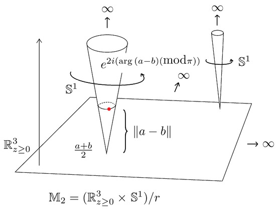
Figure 1.
The model for .
Let ; observe that there exists a closed disk D that contains x and y in its interior; then, is a neighborhood of in . Given that is a compact set, it follows that is a Hausdorff and a locally compact topological space; then, it is possible to consider the Alexandroff’s compactification, denoted by . The point added is denoted by ∞ (observe that this point will correspond to the pair of points in , for each ). Note that in , the sets such that are mapped by to an open topological disk. Hence, the Alexandroff’s compactification of such a set will be homeomorphic to . Moreover, observe that the set of singletons together with the point ∞ in is homeomorphic to .
3. Extension of the Möbius Transformations to the Space
In this section, we will define how a Möbius transformation extends to the space . We will examine how the domains of these extended maps vary based on the specific Möbius transformation being considered. Additionally, we will describe the extensions to of the maps outlined in Theorem 1, which will serve as a set of generators for all the extensions of Möbius transformations.
Let be a Möbius transformation in the Riemann sphere, define in the second symmetric space , the function given by
In particular, observe that if , then ; hence the geometry of T in will be reflected in . Since the transformation T has an inverse map , it is easy to see that in some appropriate domains, and are the identity maps.
Observe that we can use the homeomorphism to translate the definition of to ; that is, we can conjugate the map in some appropriate domain via to obtain a map in . So, from now on, by convention, for any object X in , we will use for the object in generated by X and for the corresponding object in the model .
Recall that a Möbius transformation T has at most two fixed points, and let us assume that T does not fix the point at infinity in the Riemann sphere. First, suppose that T has only one fixed point ; then, the map also has as its only fixed point; meanwhile, if T fixes two distinct points, and , then has three fixed points: .
As the map T is defined in , we need to consider the image and pre-image of the point at infinity, that is, and . Let us define the sets and ; then, we have our first result for the map .
Lemma 1.
For any Aut, the map is a homeomorphism.
Proof.
Assume that . First, let us prove that is a bijection. Let and be two points in , such that ; then, it follows that . If , then for which ; therefore ; if now , then , and then or ; in the former case, , and in the latter case, . In any case, we have that since T is a one-to-one map, for which it follows the injectivity of .
It is clear that for any pair of point , neither equal to , there are points such that and , by the surjectivity of T, and therefore is onto. Now, observe that is the inverse map of .
Finally, to establish the continuity of the map , observe that and , so by the continuity of T and the characterization of the open sets in the Hausdorff topology on , we have the result. □
Observe that if , then the map can be defined in all as in relation (1), and it is a homeomorphism there. For a general map , we can think of the action of in as follows. For any , we define the cone of vertex at w as the set . Let and . Then, acts sending the cone with vertex at one-to-one to the cone with vertex at , since , for any . We have the following result using the same arguments in the proof of Lemma 1.
Lemma 2.
Let be an element in Aut; then, the map is a homeomorphism, for any .
Some special cones need to be considered in the definition of . Suppose that is a fixed point of T; then, the cone is invariant under , that is, is a homeomorphism from to ; when T has two fixed points and , the two cones and intersect each other in the other fixed point of .
So far, we have defined only in (and then only in ), so we need to extend the definition of . Observe that the set where is not defined yet, is precisely the cone , which will be called the singular cone for T, and the other cone will be called the singular value cone for T. For , we define the function as follows:
Remark 4.
Since T is a bijective map in , we have that is a bijection from to . Also, observe that in the cone , the map continuously sends circles at some particular height to topological circles in . Moreover, sends points in the cone close to the vertex to points in the cone close to infinity, and points in close to infinity to points in close to the vertex .
In this way, we have defined in and therefore in all , since was already defined in . Moreover, . Thus, we have extended the definition of to with image , so naturally, we can extend the definition of to , sending and . Using the notation established thus far, we have the following result.
Theorem 8.
Let be a Möbius transformation in the Riemann sphere. Then, the map is a bijective map, continuous in and continuous in .
Proof.
By Lemma 1, the map is a homeomorphism in . As in a bijective way by Equation (2), and and , we conclude that is a bijection. By Remark 4, we see that is continuous within . □
Remark 5.
Since by Lemma 1, the map is a homeomorphism, any extension of the map in must have image . If we consider a sequence of points that converges to a point in and consider the open set in that contains the point , for some , then there exists such that if , it follows that . Hence, for all , and or and ; then, there are sequences of complex points , such that , , as and for . As T is a continuous map, it follows that ; therefore, we can not have continuity for the map when we approach from points in .
Remark 6.
It seems that we can use another compactification of , different from the compactification of Aleksandrov, so that the map is a homeomorphism in this new space; we add a cone with vertex at infinity compatible with the topology of ; however, we will lose the advantages of having the model for to have a geometric description of the maps . Another possible direction is to work in the second symmetric product of the Riemann sphere , but again we lose the possible model to describe the geometry of the maps .
However, the map is bijective, so we can define the set of transformations , where is defined as before. Hence, the set is a group with the composition of maps as its group operation. If and are two Möbius transformations, then we see that is well-defined in all . We will explore the structure of this group in a future manuscript.
Generators of
We will show now that all the maps in are compositions of the following four maps:
- (i)
- , ;
- (ii)
- , for ;
- (iii)
- , ;
- (iv)
- , .
Observe that , , and are homeomorphisms defined in all . Meanwhile, is defined at all points , with , but we can extend the definition of in its singular cone as in relation (2), that is, , for , and observe that for J its singular cone coincides with its singular value cone.
Proposition 1.
Let S be a map in ; then, S can be expressed as a composition in some order of the maps , , , and .
Proof.
Let Aut such that , and assume that . If , we know that , where y , hence it is straightforward to see that .
Now, when , , where . By the first part of the proof, , for some , and . Therefore . Note that the previous decomposition of even works for the singular cone , take , then . □
Let us analyze the geometry of these generators maps in the space . In order to do that, let us work on the model of . Since is a homeomorphism, we can conjugate any map to a map , that is, , extending the definition to infinity in a natural way. In particular, the elements of can be thought of as acting in , so in some cases, we will not make a distinction if the context is clear.
Let us start with the map , , and the analysis for the other maps will be similar. In this case, the conjugation gives a map such that ; the left side composition satisfies that
and the right side composition is equal to
then the next result follows directly.
Proposition 2.
The map acts as follows: , for , and .
As a result, we can determine the geometry of the map in , stated as follows.
Corollary 2.
The map acts conjugated as a double rotation with the same angle; this double rotation moves a point around a topological torus.
Proof.
Just observe that since is conjugated to , and by Proposition 2, , the orbit of the point remains at the same height and the first and third coordinates are rotated by the same angle, so the result follows. □
Similarly, we can determine the action of the corresponding maps and in the space .
Proposition 3.
The map acts as follows: , for , and .
Proof.
From the conjugation , we obtain that
from where it follows the claim, observing that . □
Using the definition in [13] of a topological attractor, we have the following result.
Corollary 3.
The point with coordinates is a fixed point of , which is a global topological attractor for the dynamics of when .
Proof.
Recall that s is the relation defined by for all , so all points can be identified to the point . It is clear that is a fixed point of . By Proposition 3, the map is defined as ; then, iterating this map, we obtain that , and since , it follows that , as . □
Proposition 4.
The map acts in the following way , for , and .
Proof.
From the conjugation , we obtain that
from where it follows the claim. □
The next result follows directly from Proposition 4.
Corollary 4.
The orbit of every point in under the map goes to infinity.
Finally, let us analyze the action of the map on . Using the conjugation , we get, first of all for , that
On the other hand, ; hence, , where , , and , are the complex numbers that depend of u as in Remark 3.
In the cone , we get that
That is, , for and . In this way, we can prove the following.
Proposition 5.
The map satisfies that , the identity map in the model of .
Proof.
For , we have that ; then, as , the result follows. In the cone , just notice that ; conjugating with the map, we have the result. □
4. Transitivity of
In this section, we will present several results regarding transitivity in the space . Let us start with two triples of distinct points in , that is, and ; then, we can consider the triples of distinct points in : , , , and . The first instance of transitivity is the following.
Proposition 6.
If and are triples of distinct points in , then there is a unique such that , for all , with .
Proof.
By Proposition 3, there is Aut such that , for ; then, , for all , with .
Suppose there is another element in such that . Consider the image of the first point, then, there are two cases. If , then , and taking one of the other two points in , we see that . By Proposition 3, we have that and therefore . In case , then , but we have that , which is a contradiction since ; this finishes the proof of the uniqueness of the map . □
Using the same argument as in the proof of the uniqueness in the previous result, we obtain the next Corollary.
Corollary 5.
If fixes three distinct point of the form , then is the identity map.
We can again use the 3-transitivity of Aut and the arguments of the proof of Proposition 6 to prove the following result.
Proposition 7.
Consider two pairs of points , and , in with and ; then, there is a unique such that and .
As a corollary, we obtain that the Möbius transformations in act transitively in the set of cones .
Corollary 6.
Let and be two singletons in . Then, there exists such that ; that is, is transitive in .
Proof.
Consider different points , and , ; by the 3-transitivity of Aut, there exists a transformation such that for . Hence, , , and . Let be a point in , with ; then, ; for points , we get . □
For general points in , we can prove the 2-transitivity of the set if these points combined have the same cross ratio.
Proposition 8.
If and are pairs of distinct points in , such that the cross ratio of is equal to the cross ratio of , then there is such that and .
Proof.
By Proposition 5, there exists Aut such that , for ; then, and . □
4.1. Transitivity of Möbius Bands
Let us consider the family of Euclidean circles in and the family of lines in ; remember that Aut sends into itself; in fact, the action is transitive there.
We have observed that is homeomorphic to a Möbius strip; then, is a Möbius band for any . Moreover, passing to the model , we can see that is a Möbius band that intersects the subset of exactly in C.
It is not difficult to see that is homeomorphic to a semi-plane in the model , for any ; in fact, .
Lemma 3.
Let K be an element in ; then, for any map S in , the set is homeomorphic to a Möbius strip or homeomorphic to a semi-plane in the model .
Proof.
Let S be an element of ; then, the corresponding map Aut (that is, ) satisfies that is a Euclidean circle or a line in . Assume that is an element of ; the proof for the other case is similar. When passing to the model , consider the set .
First, if is a Euclidean circle, then is a Möbius band. Since and , for any , it follows that .
Now, assume that is a line in ; this happens if and the point is a point on C. Remember that in this case , and ; then, we only consider the image of ; that is, is a complete line since . It follows that is still a whole semi-plane, and once again, using that , we get that , which concludes the proof. □
Now we will prove transitivity for a family of Möbius strips in . Consider the set ; that is, consists of Möbius bands and semi-planes generated by Euclidean circles and lines in , respectively.
Theorem 9.
The set acts transitively on ; that is, if , , then there exists such that .
Proof.
Let and be two elements in . Let , be two different points in , and let , be two different points in ; then, are in the same Euclidean circle or in the same line in that generates the Möbius strip or the semi-plane . The same holds for ; i.e., they are in the same Euclidean circle or in the same line in that generates the Möbius strip or the semi-plane .
Notice that since , are different points, then there are at least three different complex numbers in the set , and the same happens in the set . According to Proposition 3, there is a unique Möbius transformation S that sends the three different points in A into the three different points in B. Since three points are sufficient to determine a circle or a line, then , and then . □
The next result characterizes the sets in using the cross-ratio.
Corollary 7.
Let be an element in , and let be a point in . Then, .
Proof.
First, observe that is a line in . The set is generated by a Euclidean circle or a line K in . Let T be the Möbius transformation such that ; then, if , it follows that . By Theorem 5, , and the result follows. □
4.2. Inversion in Möbius Strips
Let C be a circle in given by the equation , with , . If , then C is a Euclidean circle in the complex plane; hence, there exists a transformation in the complex plane that fixes C given by
which is called the inversion in C. This transformation fixes point-wise the set C, sends the center of C to infinity and vice versa, and is the identity map. Moreover, if Aut, then is another circle, and we have .
Given a Euclidean circle C in , we have that is homeomorphic to a Möbius strip, for which we can define its inversion as follows. Let be the corresponding Möbius band in the model , and let such that , where is given by , for , and , where is the center of C. We call the map the inversion in the Möbius band . Then, we have the following properties for the map , taking as in (3) from now on.
Proposition 9.
The map fixes point-wise the Möbius strip , and is the identity map in .
Proof.
As fixes the set C point-wise, it follows that if . Thus, , we conclude that fixes point-wise.
The second statement follows from the fact that , for any ; and . □
Remark 7.
For any complex number z, we know that ; then, it follows that is a fixed point for ; that is, not only fixes the Möbius strip , but it has infinitely many other fixed points. Observe that these points correspond to infinite rays coming out from the manifold boundary of the fixed Möbius strip, and these rays do not intersect. Therefore, the fixed set is homeomorphic to a real projective plane minus a point. Moreover, every point in is a fixed point or a periodic point of period 2 under .
Now, let us consider two Möbius bands , in , so we know that there is a Möbius transformation T such that ; then, the next result follows.
Proposition 10.
Let and be two inversions in the Möbius bands and in , respectively. Then, they are conjugated in the subset of .
Proof.
Just observe that there is a Möbius transformation such that . Since , it follows that in , and then after conjugating with the map , we obtain in . □
Note that we can extend the conjugation to , since we must have that
and then use the map . Notice that when is a line, we have ; then, .
In particular, consider the real line ; then, for any Euclidean circle C, we can send C to by a Möbius transformation , then the point since . Thus, , where . In , we get that , and , since , where as . In this way, we have defined the conjugation in all , and then we can pass to .
Theorem 10.
For any in , the inversion in is conjugated to the map , given by , for , and .
Proof.
Let T be the Möbius transformation such that , and we assume that C is a Euclidean circle; the case when C is a line is similar. Since , it follows that the map is defined in as . Thus, is defined in ; using the conjugation , we obtain that
is equal to , and the result follows in .
To complete the proof, observe that for points , we get that
but since , then , and , so we can conclude that for , as well. □
5. Conjugacy Classes in
Given Aut, it is well-known that if T is different from the identity, then T is conjugated to for some , where if and , otherwise. In this section, we will extend this result for maps in and show how the corresponding maps act in .
5.1. Parabolic Maps
Let be a Möbius transformation with only one fixed point at ; then, T is called a parabolic transformation, and it is conjugated to the map . Let S be the Möbius transformation that conjugates T and , such that , so for some . In order to see the conjugation in , we need to consider the singular cones of T and S.
First, consider the singular cone of S, that is, coincides with the cone ; then, is given by . So the conjugation map in is given by ; then, we define in as . Similarly, in the singular cone of T, we have , and we would like the last quantity to be equal to ; then, we define in .
In any other cone , with , we have that , in , that is, . Using the relation , we can conjugate the action of in to the action of in .
Remark 8.
In , we obtain that
Remark 9.
Meanwhile, in , we get, for and
Setting , we get the following result.
Theorem 11.
Let be a map with only one fixed point; then, W is conjugated to the map given by , where , and .
Proof.
As W has only one fixed point in , then for some parabolic map . Since T is conjugated to the map , then the result follows by Proposition 4, taking , since for any , the map . □
Corollary 8.
The orbit of every point in under a parabolic map in tends to the fixed point of the map.
Proof.
Let us start in ; since by 8, it follows that
then , as n goes to infinity. Since , then . The argument is the same for points in and , by Remark 9 and Theorem 11. □
5.2. Hyperbolic, Loxodromic and Elliptic Maps
Now, let be a Möbius transformation with two fixed points and . It is conjugated to the map with , using a Möbius transformation S such that and ; that is, we can take . If and , then T is called hyperbolic; otherwise, T is called loxodromic. If , the map T is called elliptic. As in the parabolic case, to find the map that is conjugated to , we need to consider some special subsets of and some generalities about the conjugation in this setting before analyzing the different cases.
Let us consider three special cones: the singular cone of T, and the cones and , where the singular cone of S coincides with . Observe that , , for , and . For points in , we would like to have , so we define in . In the same way, in we need to happen that , so we define in . Finally, if we set and , then in we must have , so we define in .
For , we have that ; that is, in any cone . Using the relation , we can conjugate the action of in to the action of in .
Proceeding as in Remarks 8 and 9, we obtain the conjugation in the corresponding domains. In , we obtain that
and, in we get that
Meanwhile, in , we get, setting and
5.2.1. Hyperbolic and Loxodromic Maps
Let be a Möbius transformation conjugated to with . Let . Then, we get the following result.
Theorem 12.
Let be a hyperbolic map. Then, is conjugated to the map given by , for , and .
Proof.
From the conjugation , we obtain that
from where it follows the claim. □
By the action of in , that is, by Equations (4)–(6) and by Theorem 12, as well as Remark 2, we conclude the following result.
Corollary 9.
The orbit of every point in under a hyperbolic or loxodromic map in tends to one of the fixed points of the map and away from the other fixed point.
As in the classical theory of Möbius transformation, we can make a geometric distinction between hyperbolic and loxodromic elements in . Remember that a hyperbolic Möbius transformation T always has an invariant disc in the complex plane, that is, it leaves its boundary invariant, so the corresponding map must leave a Möbius strip invariant; meanwhile, a loxodromic element can not leave any Möbius band invariant.
5.2.2. Elliptic Maps
Let be a Möbius transformation with two fixed points and conjugated to the map with but . Consider . We get the following.
Theorem 13.
Let be a map such that T is an elliptic map. Then is conjugated to the map given by , for , and .
Proof.
The proof follows the same lines as before; from the relation , we obtain that
from where it follows the claim. □
By the final part of the Remark 4 and the previous Theorem, for an elliptic map T, the set has no limit, for any point , with .
We recall that the period or order of a Möbius transformation T is the least positive integer m such that is the identity map if such an integer exists. So, we have the next consequence of Theorem 13.
Corollary 10.
If T is a non-identity Möbius map with finite period n, then the map conjugated to satisfies that is the identity map in .
Proof.
Since T has a finite period, then it is an elliptic map conjugated to the map , with , , and . By Theorem 13, is conjugated to the map given by , for , and . Then,
which proves the claim. □
We can say a little more about elliptic maps with finite period. Since is the identity map, we have that , for . Recall that , and then since is the identity. Hence, for , we have that , and then ; therefore, . To get the identity, we need to iterate the map times, that is, . Thus, for any elliptic Möbius map with a finite period, we get a map in that also has a finite period, which gives us an example of a finite subgroup in .
6. Conclusions and Future Work
For any Möbius transformation in the Riemann sphere, we have defined a map in two steps. For the singular cone of T, , we have defined as , and for , we have , and then we extended it to ∞ sending and . In this way, is a bijection, and it is a homeomorphism if we restrict the map to and , separately. The lack of continuity in between is not an impediment to extend several classical results of the set of Möbius transformations in the complex plane to the set of maps such as properties of transitivity, decomposition in generators, and conjugation to simple maps.
We describe the generators of , proving how they behave geometrically in the model , which gives a better understanding of the orbits under these generators, so we observe several similarities with the geometry of the orbits of points under classical Möbius transformations.
Another important feature that we can extend are the transitivity properties of the set , not only at the points in but also in the so-called cones. Moreover, we prove transitivity in a large set of Möbius strips contained in , we give a characterization of these Möbius bands using cross-ratio, and we prove that the concept of inversion in a Euclidean circle can be extended to this set of Möbius strips, given a geometric description in of this new inversion map.
The conjugacy classes in Aut are important since they give a geometric classification of the Möbius transformations in the Riemann sphere. We show that we can extend this geometric classification in our setting, describing geometrically the representatives of every conjugacy class.
In summary, we demonstrate in this paper that the classical theory of Möbius transformation can be extended not just to or but to other topological spaces, as we have done for the second symmetric product of the complex plane.
In future work, we would like to explore the group properties of the set and extend the action of the special linear group with real coefficients, PSL, in to .
Author Contributions
Conceptualization, G.H., U.M.-F. and R.V.; methodology, G.H., U.M.-F. and R.V.; formal analysis, G.H., U.M.-F. and R.V.; investigation, G.H., U.M.-F. and R.V.; writing—original draft preparation, R.V.; writing—review and editing, G.H., U.M.-F. and R.V. All authors have read and agreed to the published version of the manuscript.
Funding
This research received no external funding.
Data Availability Statement
Data are contained within the article.
Conflicts of Interest
The authors declare no conflicts of interest.
References
- Tuffley, C. Finite subsets spaces of S1. Algebr. Geom. Topol. 2002, 2, 1119–1145. [Google Scholar] [CrossRef]
- Borsuk, K.; Ulam, S. On symmetric products of topological spaces. Bull. Am. Math. Soc. 1931, 37, 875–882. [Google Scholar] [CrossRef]
- Illanes, A.; Nadler, B. Hyperspaces: Fundamentals and Recent Advances; Marcel Dekker: New York, NY, USA, 1999. [Google Scholar]
- Meyerson, M.D. Balancing acts. Top. Proc. 1981, 6, 59–75. [Google Scholar]
- Morales-Fuentes, U.; Villanueva-Segovia, C. Rectangles inscribed in locally connected plane continua. Top. Proc. 2021, 58, 37–43. [Google Scholar]
- Greene, J.E.; Lobb, A. The rectangular peg problem. Ann. Math. 2021, 194, 509–517. [Google Scholar] [CrossRef]
- Jones, G.A.; Singerman, D. Complex Functions. An Algebraic and Geometric Viewpoint; Cambridge University Press: Cambridge, UK, 1987. [Google Scholar]
- Beardon, A. The Geometry of Discrete Groups; Springer: New York, NY, USA, 1983. [Google Scholar]
- Macías, S. Topics on Continua, 2nd ed.; Springer: Berlin/Heidelberg, Germany, 2018. [Google Scholar]
- Vaughan, H. Rectangles and Simple Closed Curves; Lecture; University of Illinois at Urbana-Champaign: Champaign, IL, USA, 1977. [Google Scholar]
- Schwartz, R.E. Rectangles, curves and Klein bottles. Bull. Am. Math. Soc. 2022, 59, 1–17. [Google Scholar] [CrossRef]
- Morales-Fuentes, U.; Valdez, R. Quadratic dynamics in the second symmetric product of ℂ. Dyn. Sys. 2024, Submitted. [Google Scholar]
- Milnor, J. Dynamics in One Complex Variable, 3rd ed.; Annals of Mathematics Studies 160; Princeton University Press: Princeton, NJ, USA, 2006. [Google Scholar]
Disclaimer/Publisher’s Note: The statements, opinions and data contained in all publications are solely those of the individual author(s) and contributor(s) and not of MDPI and/or the editor(s). MDPI and/or the editor(s) disclaim responsibility for any injury to people or property resulting from any ideas, methods, instructions or products referred to in the content. |
© 2025 by the authors. Licensee MDPI, Basel, Switzerland. This article is an open access article distributed under the terms and conditions of the Creative Commons Attribution (CC BY) license (https://creativecommons.org/licenses/by/4.0/).