Article

Route Optimization of Hazardous Material Railway Transportation Based on Conditional Value-at-Risk Considering Risk Equity

School of Business, East China University of Science and Technology, Shanghai 200237, China
*
Author to whom correspondence should be addressed.
Mathematics 2025, 13(5), 803; https://doi.org/10.3390/math13050803
Submission received: 22 January 2025 / Revised: 20 February 2025 / Accepted: 25 February 2025 / Published: 27 February 2025
(This article belongs to the Section D2: Operations Research and Fuzzy Decision Making)

Abstract

:
Rail transportation of hazardous material (Hazmat) involves low-probability, and high-consequence risks, requiring strategies that mitigate extreme accident impacts while ensuring fair risk distribution. To address this, we introduce conditional value-at-risk with equity (CVaRE) into railway Hazmats risk assessment, enabling flexible decision-making that balances risk minimization and equity considerations. Unlike conventional models that focus solely on risk reduction, CVaRE incorporates a risk equity goal, ensuring a more balanced distribution of risk across transportation routes. This study develops a novel CVaRE model that replaces fixed threshold constraints with a dynamic risk equity goal, providing greater flexibility in risk distribution adjustments. A k-shortest path-based algorithm was designed to balance extreme risk minimization with equitable risk allocation in route selection. A case study on the Yangtze River Delta railway network validates the model, demonstrating that moderate cost increases can significantly reduce extreme accident risks while achieving fairer risk distribution. Findings also show that direct transportation improves risk equity over transfer-based routes, highlighting the importance of strategic route planning. This research offers practical decision support for transport companies and regulators, helping optimize routes while ensuring cost efficiency and regulatory compliance. It also provides a scientific foundation for risk-equity-based policies, promoting safer, more sustainable Hazmat railway transportation.

1. Introduction

Hazardous material (Hazmat) transportation, despite its inherent risks, remains a crucial component of industrial production and supply chain logistics. As a key mode of transport, railways play a significant role in ensuring the efficient and safe delivery of Hazmat. Over the past two decades, both infrastructure and regulatory frameworks for railway Hazmat transportation have gradually matured. From 2011 to 2020, approximately 114,005 train accidents were reported, involving 70,432 Hazmat carrying cars in the United States. Of these, 6854 cars were damaged or derailed, with 425 releasing hazardous material, averaging 42.5 Hazmat release incidents per year [1]. In China, annual hazardous chemical shipments reached 1.8 billion tons by 2022, with 180 million tons transported by rail [2]. On 23 May 2017, a hazardous chemicals transportation explosion occurred in a tunnel on the Zhangshi Expressway in Baoding, Hebei, resulting in 15 deaths and damage to vehicles. In another incident, on 3 February 2023, a freight train carrying hazardous material derailed in East Palestine, Ohio, USA, causing the death of nearly 44,000 animals, according to data from the Ohio Department of Natural Resources. Though Bubbico et al. [3] proved that it is safer to transport Hazmat by rail, Hazmat events still have the characteristic of low probability-high consequence, which makes effective risk assessment always a problem. Expected consequence (Traditional Risk model) is risk-neutral, so it is impossible to develop a risk aversion route that would prevent high-consequence events.
There is abundant literature published on the risk assessment of Hazmat transportation. Abkowitz et al. [4] established a Perceived Risk (PR) model by introducing the risk preference parameter q into a Traditional Risk (TR) model to reflect the degree of risk preference of decision-makers. As we have found, people’s risk aversion to disasters such as hazardous material accidents is objective, and their aversion to the consequences of larger accidents is deeper than that of events with high probability and small consequences; hence, the model is very close to realistic decision-making. However, it is difficult to determine an appropriate risk preference parameter q in actual production and scientific research activities. Erkut and Ingolfsson [5] introduced three different catastrophe avoidance models, namely minimizing the maximum risk, minimizing the variance of results between routes, and an explicit disutility function. Liu et al. [6] used a Gaussian Plume Model to estimate the population exposure risk for hazardous material road transportation, considering environmental risk under time-varying conditions. With the help of or partially improving these risk assessment models, scholars have performed research on route selection and location decision-making for hazardous material road transportation and even multimodal transportation under various scenarios [7,8,9,10,11].
Kang et al. [12] proposed a value-at-risk (VaR) model to assess the risk of dangerous goods transportation. Fang et al. [13] further demonstrated the application of VaR in multi-hazmat railcar routing, highlighting its effectiveness in optimizing route risks. Meanwhile, conditional value-at-risk (CVaR), as an extension of VaR, quantifies extreme losses exceeding the mean value of VaR [14]. Since then, scholars have studied the use of CVaR for dynamic route and scheduling decisions in Hazmat transportation networks [14,15]. The CVaR is originally applied for financial portfolio optimization in the financial field [16]. Based on the widespread application of CVaR in risk-averse decision-making, Huang et al. [17] constructed a supply chain transportation network to analyze suppliers’ risk aversion under stochastic pricing and information asymmetry. They proposed an emergency quantity discount contract to coordinate the supply chain. Ma et al. [18] integrated CVaR into a blockchain-enabled supply chain finance system, investigating revenue optimization under centralized and decentralized decision-making models, thereby demonstrating CVaR’s versatility in complex scenarios. In hazardous material transportation, extreme accident events—though low in probability—can result in catastrophic consequences, including environmental damage, human casualties, and significant financial losses. Traditional risk measures often fail to capture such tail-end risks, making them inadequate for hazardous material logistics. CVaR, by focusing on the expectation of extreme losses, provides a more robust framework for decision-making under uncertainty. Hosseini and Verma [19] proposed a CVaR-based risk assessment methodology for rail Hazmat shipments and even provided a clear definition of CVaR for these shipments. Zhong et al. [20] proposed a new model that includes conditional value at risk with regret (CVaR-R) as a risk measure that considers both the reliability and unreliability aspects of demand variability in the disaster relief facility location and vehicle routing problem. Su [21] incorporated CVaR risk measurement into Hazmat network design and achieved good research results.
In recent years, with the occurrence of Hazmat accidents, the problem of risk unfairness has aroused widespread concern among the public and society. Scholars use two ways of modelling to solve the problem of risk equity: one is to directly limit the risks related to the relevant population area by setting thresholds as constraints [22,23,24], and the other way is to implement risk equity by setting risk equity goal [25,26]. Furthermore, Fontaine et al. [27] proposed a new population-based risk definition and an objective function for achieving risk equilibrium. Liu and Liu [28] achieved risk equity in hazardous material transportation network design by computing risk differences between links under uncertain demand. Liu et al. [29] enhanced risk equity by applying a threshold-setting method to minimize disparities in population exposure risks among road segments while considering time-varying risk factors. Hosseini and Verma [22] proposed an analytical framework that makes use of a CVaR measure of risk to generate the shortest risk shipment routes while promoting risk equity in both the arcs and the yards of the railway network. However, the approach that they used setting risk equity constraints for each yard and each arc is no longer popular. Because it is difficult to determine a reasonable risk threshold in large-scale instances, this method has been gradually replaced by setting risk equity goals in the recent literature.
Using CVaR minimized as the goal requires paying attention to serious consequences to achieve risk aversion. This will make the system’s decision to avoid extremely high consequences. However, this goal can only ensure that the accident consequence of a single road section or node is minimized, and it cannot achieve a balanced distribution of risks between road sections and nodes. Setting a risk equity goal should enable groups that are susceptible to risk unfairness (those groups are generally located geographically on risky routes or near stations) to reduce risk as much as possible. Combining it with the goal of minimizing CVaR means so the overall risk is minimized, but also partial risk reduction must be achieved. This can better be achieved by avoidance. Therefore, we propose conditional value-at-risk with equity (CVaRE) as a combination of CVaR and risk equity goal, while reducing the frequency of extremely high consequences and higher risk.
This article has made the following contributions to solve the above problems:
  • We introduce CVaR into risk assessment in railway transportation scenarios for risk aversion routes and dispatch decisions;
  • Taking into account the risk unfairness of the external public, we added a risk equity goal to the CVaR-based assessment, and proposed a new model named CVaRE;
  • We introduce a practical example and use the k-shortest CVaRE algorithm to solve the problem model, generating the optimal solution. This can serve as a guide and reference for railway hazardous material transportation dispatch decision-makers.
The remainder of this paper is organized as follows: In Section 2, we define the research questions and basic assumptions, give the notations of sets, parameters and variables, and provide the basic definition of CVaR and the scenarios in this article. Section 3, provides a direct transportation model, a transfer transportation model, and finally, an outline of solution methodology based on the k-shortest path algorithm. Section 4 uses the railway infrastructure of railway operators to generate actual-scale calculation examples, which are solved and analyzed to obtain management insights. Conclusions and directions of future research are outlined in Section 5.

2. Problem Description

2.1. Assumptions and Notations

2.1.1. Model Assumptions

Hazmat railway transportation involves moving hazardous material between origin–destination (O-D) pairs while optimizing risk minimization, cost efficiency, and risk equity. This study focuses on applying CVaR and CVaRE to determine optimal railway transportation routes while balancing trade-offs between safety, cost, and equity in risk distribution.
The key assumptions in our model are as follows:
  • Fixed transportation network: The railway infrastructure, including yards and routes, is predefined and does not change dynamically.
  • Probability-based risk estimation: Accident probabilities and consequences are derived from historical incident reports and regulatory guidelines.
  • Travel times and accident probabilities: Assumed to be known and constant, ensuring computational efficiency but ignoring real-world uncertainties.
  • Time window constraints: Predefined operational time windows are enforced to ensure safe and timely railway arrivals, maintaining scheduling reliability while balancing efficiency and risk management.
  • Generalized hazmat risk representation: Risk estimation is based on historical data and predefined exposure factors, without differentiating between Hazmat types.
In the railway transportation system, the physical infrastructure includes railway yards and tracks. Any two railway stations are connected by tracks, and a series of service sections and intermediate stations constitute the itinerary that the railcar can use for its itinerary. There are two ways to transport hazardous materials: direct transportation and transfer transportation. Direct transportation does not stop at any station, and transfer transportation (as Figure 1 depicts) involves stopping at specific railway yards, referred to as marshalling yards, where railcars are reclassified and reassembled before continuing their journey.
A marshalling yard is a specialized railway facility where railcars are sorted, grouped, and rearranged according to their destinations. In the context of hazardous material transportation, marshalling yards play a crucial role in regulating freight flow, ensuring the proper handling of dangerous goods, and minimizing risks associated with rail transfers. Proper reclassification at marshalling yards helps optimize train operations while maintaining safety and regulatory compliance.
The problem we need to solve is the train transportation route and re-marshalling plan of the railway company, which regularly transports Hazmat between different origins and destinations, and needs to ensure that the needs are met. Therefore, the goal is to use the conditional value-at-risk method and conditional value-at-risk with equity method to determine Hazmat railway transportation routes and possible regrouping stations and plans so that hazardous material risks are minimized and distributed fairly among the railway network.

2.1.2. Notations

The railway transportation network is represented by a graph G = ( Y , A , V ) , where Y is the set of yards. A is the set of arcs in the network, representing the connections between yards or between a yard and a marshalling yard. V is the set of railway shipments, which flow between railway yards or between yards and marshalling yards. This network structure supports the transportation of hazardous material by modelling both direct shipments and transfer shipments through intermediate marshalling yards. The specific definitions of the symbols are provided below:
Sets and indices
Y Set of yards, indexed by i, j, k
Y M Set of marshalling yards, indexed by k, Y M Y
A Set of arcs in the network, indexed by (i, j), (k, j)
V Set of railway shipments between railway yards (or yard and marshalling yards), indexed by v
Y v Set of yards in service of shipment v
A v Set of arcs in service of shipment v
Parameters and Variables
C i j v Cost of moving a Hazmat container on arc (i, j) in shipment v
R i j v Exposure risk of moving a Hazmat container on arc (i, j) in shipment v
R k v Exposure risk of using yard k for a Hazmat container in shipment v
O ( v ) Origin of shipment v
D ( v ) Destination of shipment v
N ( v ) Non-negative integer, number of Hazmat containers in shipment v
α Confidence level, but also represents the level of risk aversion of suppliers
c i j v Risk consequences in shipment v on arc (i, j) in shipment v
P i j v Accident probability on arc (i, j) in shipment v
c k v Risk consequences of using yard k for Hazmat shipment v
P k Probability of accident in using yard k
y Select Route VaR Threshold Under CVaR*
x i j v 0–1 variable, whether to select arc (i, j) in shipment v as transportation section
y k v 0–1 variable, whether to select yard k as railway yard in shipment v
d k v Number of containers in shipment v unload at Marshalling yard k
D T v Delivery time associated with shipment v
t k Time for handling containers at marshalling yard k
t A Time for running on the railway route
r Impact radius of Hazmat accident
ρ i j Maximum population density of the area passed through by arc (i, j)
ρ k Population density of the area where yard k is located

2.2. Hazmat Risk Measurement Formulation Based on VaR and CVaR

CVaR is based on VaR. VaR refers to the maximum possible loss value of a certain financial asset or portfolio within a certain holding period under a certain confidence level. It focuses on a certain point of confidence, while ignoring the underlying risk beyond that point. Compared with VaR, CVaR satisfies the consistency axiom, and pays attention to the risk of exceeding the base point. Therefore, soon after scholars introduced VaR in the Hazmat transportation, they introduced CVaR into the risk assessment of Hazmat transportation.
Given that R v is the discrete random variable denoting the risk associated with O-D pair O ( v ) D ( v ) , c t v is the t t h smallest value in the set { c i j v c k v : ( i , j ) A & k Y M }, and P t v is the corresponding probability.
R v = c 0 v = 0 ,   w i t h     p r o b a b i l i t y   P 0 v ; c 1 v ,   w i t h     p r o b a b i l i t y   P 1 v ; c t v ,   w i t h     p r o b a b i l i t y   P t v ; c | A | v ,   w i t h     p r o b a b i l i t y   P | A | v .
where c 0 v < c 1 v < < c t v < < c | A | v ,   t 0 ,   1 ,   2 ,     ,   A .
Given the confidence level α , VaR is the minimal threshold level β such that the hazmat risk R v does not exceed β with the least probability of α and is expressed as follows:
V a R α v = min β | Pr ( R v β ) α
CVaR is the weighted average of VaR and the hazmat risk greater than that [30,31] is as follows:
C V a R α v = λ α v V a R α v + ( 1 λ α v ) E ( R v | R v > V a R α v )
Note that λ α v = P ( R v V a R α v ) α 1 - α , where always P ( R v V a R α v ) α
Then,
V a R α can be simplified as y, which is the minimal loss value for decision-making shipment v under the confidence level α . When 0 < α P 0 v , we define T as equal to 0; then, 0 T - 1 P t v < α 0 T P t v . Therefore, the VaR risk of O-D pair O ( v ) D ( v ) has y = V a R α v = c T v .
There is a shipment v for a specific O-D pair, C V a R α v can be written as F α . Therefore, a discrete CVaR assessment (4) for each O-D pair is established for the transportation of hazardous material. The consequences of the risk are measured by road segments; the corresponding consequence for each road segment (i, j), is c i j ; the corresponding probability is P i j ; then,
F α = y + 1 1 α ( i , j ) A v c i j v y + P i j v x i j v
Note that t + = max ( t , 0 ) .
The optimal conditional risk value for a specific O-D pair can be expressed as follows [30]:
min C V a R α v = min F α                                   v V = min ( y + E [ c i j v y ] + ) = min ( y + 1 1 α ( i , j ) A v P i j v c i j v y + x i j v )
For N is set of midpoints in the network, x i j v indicates whether to choose a route for transportation;
Ω = { x : i = O , j = N x i j v = 1 ,   i = N , j = D x i j v = 1 , j N x i j v = i N x j i v , x i j v { 0 , 1 } , ( i , j ) A } .
Because of the optimal y content y { c i j v c k v } , the optimal VaR is between the risk of the minimal road segment and the risk of the maximum road segment, and the risk values c i j v , c k v of all the road segments of v V are sorted in ascending order and defined separately as c 0 , c 1 , , c t , , c | A | , where c t is the t t h minimal value of { c i j v c k v } , C 0 = 0 . The values of y 0 { c i j v c k v } must be fixed, and the objective function becomes a linear function. Therefore,
C V a R α v = min y { 0 , c 1 , , c t , , c A } y + 1 1 α ( ( i , j ) A v P i j v [ c i j v y ] + x i j v + k Y v P k v [ c k v y ] + y k v ) .
After determining the values’ range of y, it can be converted into a linear function. Since the CVaR function is convex, it is consistent with f a + b 2 f a + f b 2 . Generally speaking, α [ 0 , 1 ) in the calculation of CVaR. From Equation (7), we can see that different y corresponding to different CVaR values, the optimal CVaR corresponds to the optimal VaR.

3. Model Establishment

3.1. Mathematical Model

In this section, we outline the model of Hazmat railway transportation system in direct transportation case and transfer transportation case.

3.1.1. Model Based on CVaR of Direct Transportation Case (Base Case)

We call the Hazmat railway transportation problem of direct transportation case (base case) problem (P). The proposed problem (P) is formulated below.
M i n v C V a R α v
M i n v ( i , j ) A v C i j v N ( v )
Subject to
C V a R α v = y + 1 1 α ( i , j ) A v P i j v [ c i j v y 0 ] + x i j v ,   ( i , j ) A , v V
j x i j v j x j i v = 1 ,   i = O ( v ) ; - 1 ,   i = D ( v ) ; 0 ,   i = N . ( i , j ) A , v V
c i j v = π r 2 ρ i j , ( i , j ) A , v V
c k v = π r 2 ρ k , k Y , v V .
The model is a bi-objective model: the objective function (8) is minimizing the total CVaR for all the shipments; (9) is to minimize the total cost of Hazmat transportation, which includes the cost of moving Hazmat on arc (i, j). Constraint (10) represents CVaR in shipment v, among them, [ x ] + = max ( x , 0 ) ; Constraint (11) is the flow balance equation for any (i, j) ϵ A. Equations (12a) and (12b) represent the accident consequences of exposure risk on arc (i, j) and yard k, respectively.
The model P is aimed at the simple direct transportation problem (there is no stopover in this type of problem). In fact, the railway has a marshalling station for the reorganization, transfer, and delivery of trains on the railway. In the strict management system of railways, the arrival and departure of hazardous material carriages can only be carried out on special railway lines and marshalling yards, so Hazmat railway transportation excludes halfway stations of the non-marshalling station.

3.1.2. Model Based on CVaRE of Transfer Transportation Case Considering Risk Equity

With the growing awareness of risk among governments and the public, it has become essential to incorporate risk equity into railway Hazmat transportation. While CVaR focuses on reducing the likelihood of extreme accident outcomes beyond a given threshold y, its ability to ensure fair risk distribution is limited, as the selection of y and α largely depends on the subjective preferences of decision-makers. To address this, we introduced a quantitative measure of risk equity based on the deviation between individual road section risk and the network-wide average risk. The network’s average risk is determined by calculating the total weighted risk divided by the sum of risk-weighted route usages. The deviation between a specific road section’s risk and this network-wide average serves as an equity measure—larger deviations indicate a more uneven risk distribution, where certain sections may bear disproportionately high hazardous material transport risks.
We define risk equity as follows:
R E v = 1 1 α ( i , j ) A x i j v [ R i j v 1 ( i , j ) A x i j v ( i , j ) A P i j m c i j v x i j v ] +
In this case, due to the operational requirements of train scheduling and logistics, the risks associated with transit yards must be considered. Traditional CVaR models primarily focus on minimizing extreme risk exposure but fail to address the unequal distribution of risk among different transportation segments. A notable attempt to integrate risk equity into railway hazardous material transportation planning was proposed by Hosseini and Verma [22], who introduced fixed threshold constraints to enforce risk equity at specific network locations. In contrast, we introduced a risk equity goal into the CVaR framework, leading to the development of conditional value-at-risk with equity (CVaRE).
C V a R E α v = R E v + min y 0 { 0 , c 1 , , c t , , c V } y + 1 1 α ( i , j ) A v P i j v [ c i j v y 0 ] + x i j v + k Y v P k [ c k v y 0 ] + y k v
The integration of risk equity into the CVaR model represents a key advancement over existing methods. Instead of solely reducing expected tail-end risks, CVaRE explicitly incorporates risk equity as an optimization objective rather than a fixed constraint. This approach enables a more adaptive and context-aware risk distribution mechanism, allowing decision-makers to balance extreme risk minimization with equitable risk allocation in real time. Traditional threshold-based methods require predefined risk caps at each node and arc, which can be challenging to determine and may not generalize well across different transportation networks. In contrast, CVaRE’s risk equity goal formulation eliminates the need for arbitrary threshold settings, providing a more flexible, scalable, and responsive solution that prevents excessive risk accumulation in high-exposure areas such as transit yards and densely populated corridors, while maintaining cost-efficiency and operational feasibility.
The proposed model (P′) is provided as follows:
M i n v C V a R E α v
M i n v ( i , j ) A C i j v N ( v )
Subject to
j x i j v j x j i v = 1 , i = O ( v ) ; 1 , i = D ( v ) ; 0 , i O ( v ) D ( v ) . ( i , j ) A , v V
Y k v t k v + t A v D T v       k Y v , v V
t k = d k v * t = ( n N ( v ) ) x i k v * t       k Y v , v V
R i j v = P i j v c i j v x i j v       ( i , j ) A v , v V
R k v = P k c k v y k v       k Y v , v V
x i j v   0 , 1 ( i , j ) A v , v V
y k v = 1 , N ( v ) < n ; 0 , o t h e r w i s e .     k Y v , v V .
The objective function (15) is minimizing total CVaRE for all the shipments and (16) is to minimize the total cost of Hazmat transportation. Constraint (17) is the flow balance equation for any (i, j) ϵ A. Constraint (18) ensures that shipment v arrives at the customer’s location within the specified delivery time. Constraint (19) represents the time for handling containers at marshalling yard k, where t is time spent processing a container. Equations (20a) and (20b) represent the risk of arc (i, j) and yard k in shipment v, respectively. The sign restriction constraints are represented in (21) and (22), constraint (22) is to determine whether to transfer shipment v at yard k.

3.2. Solution Methodology

The problem of this paper is to choose a suitable route and marshalling plan for the railway transportation of hazardous material in the network and involves the risks and costs of service endpoints and service links, and direct transportation case and transfer transportation case are modelled separately. Hence, the problem model in this paper is a two-stage plan. The first stage is to select long-distance transportation links between different O-D pairs. The second stage is to select the optimal link from the k optimal links selected in the first step according to the model conditions and determine the marshalling plan through the marshalling yard(s).
Note that the routing constraint has a multi-commodity flow structure, so a problem can be regarded as a variant of the multi-commodity flow problem, so it is an NP-hard problem. However, purely accurate algorithms can be very slow in finding the best solution to a real-size problem instance. This inspired the development of a greedy heuristic algorithm, which combines the k-shortest path algorithm tailored for the CVaRE route. As an accurate solution, it uses the available arcs and codes that have not been overloaded to maximize each Hazmat shipment. Then, we find the route with the smallest CVaRE risk and use the greedy procedure of prioritizing the transportation of hazardous material. Therefore, we use the following algorithm to simplify the process and solve the model in MATLAB-R2020a.
Stage 1
Step1.1: Sort y = c t v { c i j v c k v } in ascending order, select a certain initial point y = c 0 = 0 . It gives a new set of { c t v } where c t v c t 1 v 0 .
Step1.2: Define R i j v = N ( v ) * P i j v * c i j v , R k v = N ( v ) * P k * c k v , and set the initial values R i j 0 = 0 , R k 0 = 0 , ( i , j ) A .
Step1.3: Sort O-D pairs in ascending order in terms of v, input the origin and destination.
Step1.4: Set α = 0.9999999 . Let v ← 1.
Step1.5: Define C V a R i j v = P i j v * max ( 0 , c i j v y ) 1 α , C V a R k v = P k * max ( 0 , c k v y ) 1 α , set initial C V a R i j v = 0 , C V a R k v = 0 , ( i , j ) A .
Step1.6: For t = 0 to A perform:
f t ( v ) = min ( i , j ) C V a R i j v , using the Dijkstra’s shortest route algorithm.
If f t ( v ) < f t + 1 ( v ) , f t ¯ ( v ) = f t ( v ) .
Step1.7: Let C V a R α v = c t v + f t ¯ ( v ) , t * = arg min ( c t v + f t ¯ ( v ) ) . Hold the best route p t * ( v ) .
Step1.8: For v = 1 to v
Update C V a R i j v = 0 , C V a R k v = 0 , ( i , j ) A
If v = v stop, else vv + 1, then go to Step 1.6.
Step1.9: Calculate C V a R = v C V a R α v .
Stage 2
Step2.1: R = ( i , j ) R i j v , using the Dijkstra’s Shortest route algorithm to obtain the average risk of the road section R i j v ¯ .
Step2.2: Set R e i j v = max ( R i j v R i j v ¯ , 0 ) 1 α , set initial Re i j v = 0 .
Step2.3: Set C V a R E i j v = R e i j v + C V a R i j v , C V a R E k v = C V a R k v , and set the initial C V a R i j v = 0 , C V a R k v = 0 , ( i , j ) A . Let v←1.
Step2.4: For t = 0 to A do:
f t ( v ) = min ( ( i , j ) C V a R i j v + k C V a R k v ) , using the Dijkstra’s Shortest route algorithm.
If f t ( v ) < f t + 1 ( v ) , f t ¯ ( v ) = f t ( v ) .
Step2.5: Let C V a R α v = c t v + f t ¯ ( v ) , t * = arg min ( c t v + f t ¯ ( v ) ) . Hold the best route p t * ( v ) .
Step2.6: For v = 1 to v
Update C V a R E i j v = 0 , C V a R E k v = 0 , ( i , j ) A
If v = v stop, else v ← v + 1, then go to Step 2.4.
Step2.7: Calculate C V a R E = v C V a R E α v .

4. Computational Analysis

In this section, we first introduce the details of real-life problem examples and apply the methods proposed in the previous section to the solution of the problem. Then, we briefly discussed the comparison between our proposed CVaRE, CvaR, and TR, and analyzed the risk equity of some O-D pairs; we analyzed the results of two single goals and performed a trade-off analysis. In addition, we analyzed the solutions and provided some management insights, which can be used for policy planning purposes. Although the case study focuses on the Yangtze River Delta, the model can be adapted to regions with different geography and infrastructure by recalibrating parameters such as population density, accident probability, and transport regulations. This flexibility allows the methodology to be applicable to various regional contexts, ensuring its broader relevance for risk management and policy planning.

4.1. Problem Setting

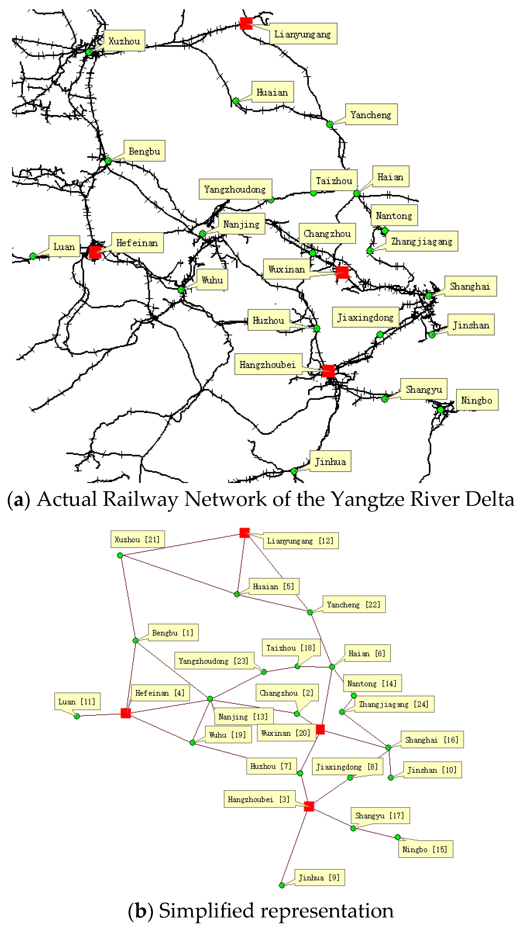
In this example, on the basis of the railway network in Yangtze River Delta of China (Jiangsu Province, Anhui Province, Zhejiang Province, and Shanghai), which is also the most developed area of the petrochemical and fine chemical industry in China. Figure 2 depicts the railway network in the Yangtze River Delta region of China based on ArcGIS data and a simplified topology of the railway network. This network has a total of 32 arcs and 24 railway yards, and from 4 yards we can carry out the Hazmat transferring and marshalling operations. There are 29 O-D pairs in the area corresponding to the yard. Different origins and destinations have differences in the daily delivery of Hazmat containers N(v). Population-related data comes from the 2019 China Urban Statistical Yearbook.
The value of α was set to 0.9999999 throughout all the analyses. The k-shortest CVaRE algorithm was implemented in MATLAB R2020a, and ran on an Intel Core i7-1165g7 CPU @ 2.80 GHz PC with 16 GB RAM.
In order to better describe the accident characteristics of different parts of the train, we divided the conditional probability into the probability of derailment, the probability of derailment of Hazmat carriage and the probability of release of Hazmat derailment. According to Verma [32], we made use of a decile-based approach to compute these probabilities (i.e., the length of a train is divided into ten equal parts):
P i j m = P ( A i j ) × u = 1 10 ε u v × ( P ( D r | A i j ) × P ( H | D r , A i j ) × P ( R | H , D r , A i j )
where P ( A i j ) is the probability that a train meet with an accident on arc(i, j);
( P ( D r | A i j ) is the conditional probability that derailment of the railcar in the u t h decile of the train;
P ( H | D r , A i j ) is the conditional probability that Hazmat carrier derailed in the u t h decile of the train;
P ( R | H , D r , A i j ) is the conditional probability of release due to derailment of Hazmat carrier in the u t h decile of the train;
ε u v represents the number of Hazmat carriers in the u t h decile of the train, it satisfies u = 1 10 ε u v = N ( v ) .
As the value taken by Hosseini and Verma [22], we determine that P i j m = l e n g t h ( k m ) × 4.57 × 10 11 × N ( v ) , P k v = 3.99 × 10 10 × N ( v ) .
In order not to lose generality in the example, we set a time window of 10 h.

4.2. Data Analysis

Table 1 depicts the optimal CVaR value and the route when the CVaR is minimized for Hazmat transportation on 29 O-D pairs. The model situation in this table should be the CVaR and route situation of direct transportation from origin to destination. For example, from origin 1 to destination 12, the optimal CVaR (minimized) is 20,256.98, and the route chosen at this time is 1→21→12.
In addition, we calculated the shortest CVaRE value corresponding to each O-D pair at this time and its corresponding route. Using Equation (13), we calculated the risk equity level R e of different O-D pairs, as shown in Table 2.
Table 2 presents the number of Hazmat containers N(v) on some O-D pairs, the value of risk equity level R e , the average risk on the shortest route on each O-D pair, and the route distance when CVaRE is minimized.
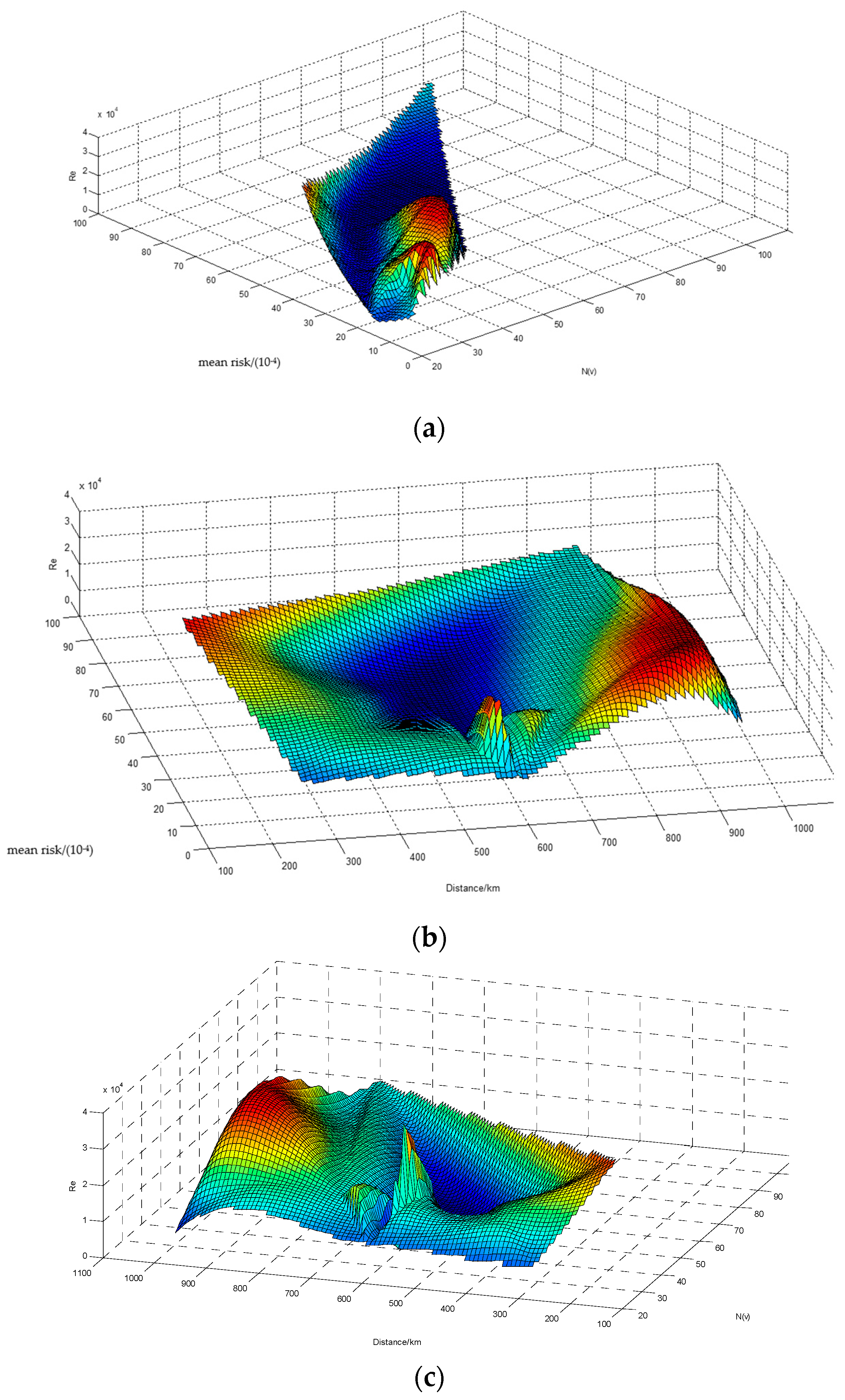
Figure 3 demonstrates the relationship between R e and several other variables in the network by using MATLAB three-dimensional images.
Figure 3a shows the relationship among R e , the number of hazardous material containers N(v), the smallest average risk. Among them, the x-axis is the number of hazardous material containers N(v), the y-axis is the smallest average risk, and the z-axis is the risk equity level R e . From Figure 3a, we find that when x ∈ (30, 50) and y ∈ (20, 40), the value of risk equity is very large, which means that the risk distribution is relatively unfair at this time.
Figure 3b shows the relationship among R e the distance of optimal CVaRE route D, average risk on the shortest route. Among them, the x-axis is the distance of optimal CVaRE route D, the y-axis is the smallest average risk R i j , and the z-axis is risk equity level R e . From Figure 3b, we can see that when x ∈ (800, 1000) or near 300, the value of risk equity is very large, that is, the risk distribution of these O-D pairs whose line distances lie in these two ranges is relatively unfair.
Figure 3c shows the relationship between R e and the number of hazardous material containers N(v) and the distance of optimal CVaRE route D. Among them, the x-axis is the number of hazardous material containers N(v), the y-axis is the smallest average risk, and the z-axis is risk-equity R e . From Figure 3c, we can obtain a similar conclusion to Figure 3b, and the N(v) in the region with high R e can be around 40 or (40, 70).
Table 3 provides the CVaR and CVaRE values of the optimal routes for the CVaR model and CVaRE model for problem P of a single O-D (18,16) under different confidence levels.
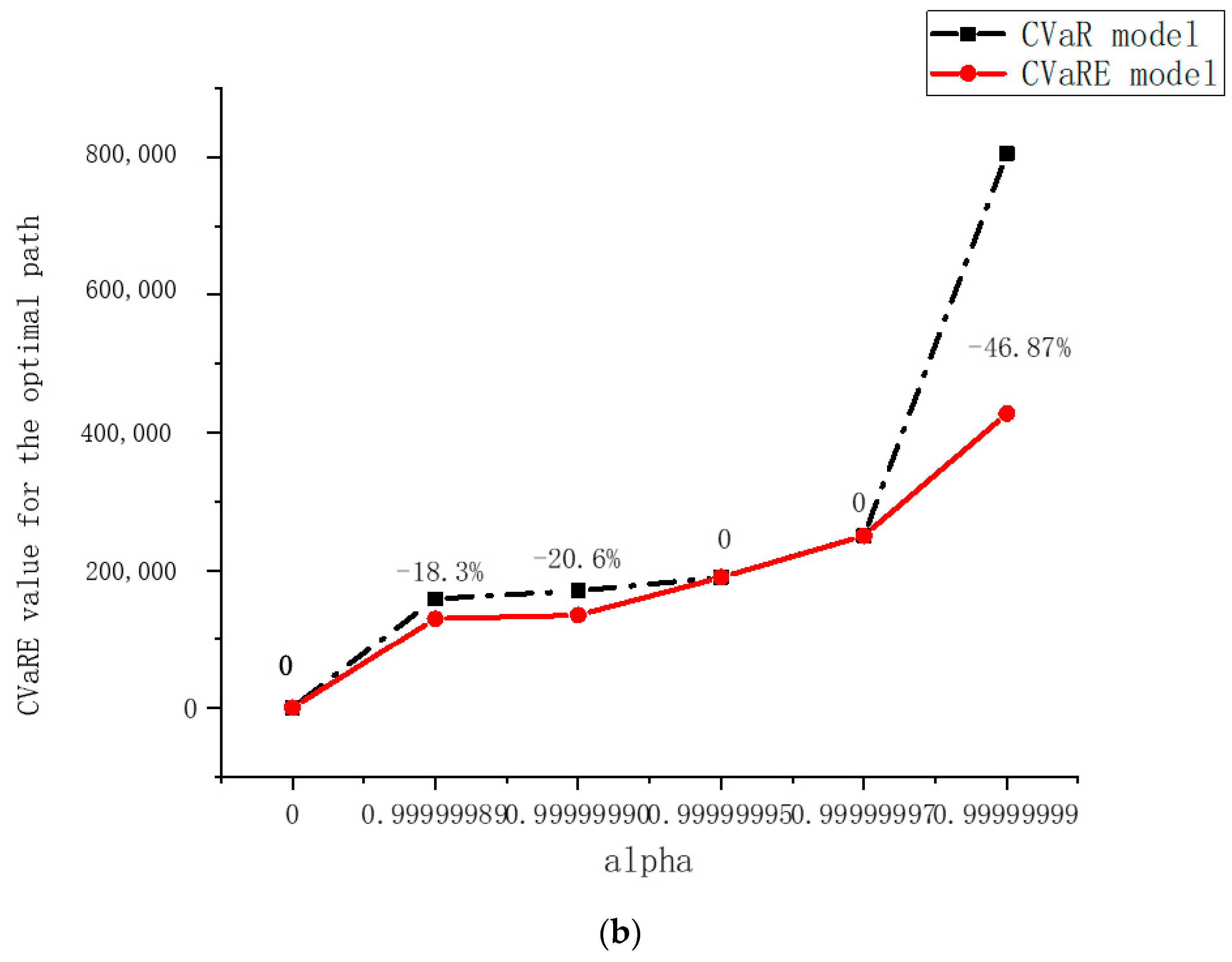
Figure 4 shows the CVaR and CVaRE values of the optimal route of the CVaR and CVaRE model in problem P under different confidence levels. The percentage data of the gap between the two is measured in data of CVaR assessment. When the confidence level α belongs to (0.99999995, 0.99999997), the optimal routes of the two models are the same. (The selected example is a normal O-D pair). When the confidence level α approaches 1, the difference between the value of CvaR and CVaRE increases sharply, while in other cases the gap is not large. It shows that CVaRE has good performance compared with CVaR and can reflect risk equity when the decision-maker is not extremely risk averse.
Table 4 describes the optimal CVaR and optimal CVaRE for direct transportation (problem P), as well as the optimal CVaRE and shortest route cost for transfer transportation (P′) with time window restrictions.
Table 4 shows the min cost solution entails a cost of around CNY 217 million and CVaRE more than 283 million, whereas the min CVaRE solution will cost CNY 236 million and CVaRE about 260 million. By spending an extra CNY 20 million, there will be a reduction of 23 million CVaRE.
In addition, we can also find that the total CVaR and CVaRE of the base case are lower than those of transfer transport, although the cost is relatively high. Moreover, after setting the time window in the base case, we found that its CVaR and CVaRE are still lower than those of transfer transportation, and the cost has dropped by about 140,000 CNY. This proves the advantages of direct transportation compared with transfer transportation in terms of risk mitigation and risk equity.

5. Conclusions

After analyzing the risks associated with hazardous material transportation, this study established a CVaR framework and introduced a novel CVaRE model. Unlike traditional models that focus solely on minimizing risk exposure, CVaRE integrates risk equity into the optimization process, ensuring a fairer distribution of risk across transportation routes. A key innovation of this model is the adoption of a risk equity goal rather than fixed threshold constraints, allowing for greater flexibility in risk distribution adjustments and eliminating the challenge of setting arbitrary thresholds. To efficiently address this issue, we developed a k-shortest CVaRE algorithm, enabling decision-makers to balance extreme risk minimization with equitable risk allocation when selecting optimal routes. Empirical results confirm that moderate increases in transportation costs can significantly reduce extreme accident risks while achieving a more balanced risk distribution. Additionally, findings indicate that direct transportation generally results in better risk equity compared to transfer-based transportation, highlighting the importance of strategic route planning in Hazmat logistics.
From a practical standpoint, the CVaRE model serves as a powerful decision support tool for transportation companies, railway operators, and regulatory agencies. For transport firms, implementing CVaRE helps optimize route selection while ensuring compliance with stringent safety regulations and minimizing liability risks. By prioritizing routes that reduce risk concentration, companies can enhance overall supply chain resilience and improve safety management. For government regulators and policymakers, the CVaRE framework provides a scientific methodology for designing risk-based policies. It enables the enforcement of equitable risk distribution, implementation of incentive mechanisms for safer routes, and development of regulatory frameworks that prevent localized risk concentration. By integrating CVaRE-based route planning, policymakers can establish a regulatory environment that aligns economic efficiency with public safety, promoting a more socially responsible hazardous material transportation system.
While this study provides valuable insights into optimizing Hazmat railway transportation, several areas merit further exploration. First, the model validation relies on historical data from the Yangtze River Delta railway network, which, while aligning well with past risk distribution trends, may not fully capture real-time variations or rare extreme events due to data constraints. Future research could incorporate standardized incident databases to empirically validate the model across diverse transportation environments. Second, while the model prioritizes risk minimization and equity, future studies could explore ways to integrate environmental impact considerations into the decision-making process, enhancing the model’s sustainability focus. Third, this study primarily focuses on railway transportation, and an important extension would be to investigate intermodal transport scenarios, such as rail-road or rail-sea integration, to understand how multiple transport modes influence risk distribution and route optimization.

Author Contributions

L.L., Conceptualization, methodology, writing and revision; S.S., data analysis, model and algorithm, writing and revision; S.L., correspondence, methodology, writing and revision. All authors have read and agreed to the published version of the manuscript.

Funding

This research was funded by the National Natural Science Foundation of China (72442009, 72032001, 72074076, 71302043); Ministry of Education, Humanities and Social Sciences Research Planning Foundation (21YJA630057).

Data Availability Statement

Data will be made available on request.

Acknowledgments

We would like to express our sincere gratitude to the anonymous reviewers for their valuable feedback and constructive suggestions, which greatly enhanced the quality of this manuscript.

Conflicts of Interest

The authors declare no conflicts of interest.

References

  1. Federal Railroad Administration Office of Safety Analysis. Available online: https://safetydata.fra.dot.gov/ (accessed on 20 January 2025).
  2. China Federation of Logistics and Purchasing. 2022 China Hazardous Chemicals Logistics. In China Logistics Yearbook; He, L.M., Ed.; China Fortune Publishing Co., Ltd.: Beijing, China, 2023; pp. 282–283. [Google Scholar]
  3. Bubbico, R.; Maschio, G.; Mazzarotta, B.; Milazzo, M.F.; Parisi, E. Risk management of road and rail transport of hazardous materials in Sicily. J. Loss Prev. Process Ind. 2006, 19, 32–38. [Google Scholar] [CrossRef]
  4. Abkowitz, M.; Lepofsky, M.; Cheng, P. Selecting criteria for designating hazardous materials highway routes. Transp. Res. Rec. 1992, 1333, 30–35. [Google Scholar]
  5. Erkut, E.; Ingolfsson, A. Catastrophe avoidance models for hazardous materials route planning. Transp. Sci. 2000, 34, 165–179. [Google Scholar] [CrossRef]
  6. Liu, L.; Wu, Q.; Li, S.; Li, Y.; Fan, T. Risk Assessment of Hazmat Road Transportation Considering Environmental Risk under Time-Varying Conditions. Int. J. Environ. Res. Public Health 2021, 18, 9780. [Google Scholar] [CrossRef] [PubMed]
  7. Qi, J.; Wang, S. LNG Bunkering Station Deployment Problem—A Case Study of a Chinese Container Shipping Network. Mathematics 2023, 11, 813. [Google Scholar] [CrossRef]
  8. Androutsopoulos, K.N.; Zografos, K.G. Modeling and solving the fuel distribution problem with unloading precedence and loading sequence considerations. Ann. Oper. Res. 2023, 332, 909–947. [Google Scholar] [CrossRef]
  9. Sun, Y. A Fuzzy Multi-Objective Routing Model for Managing Hazardous Materials Door-to-Door Transportation in the Road-Rail Multimodal Network with Uncertain Demand and Improved Service Level. IEEE Access 2020, 8, 172808–172828. [Google Scholar] [CrossRef]
  10. Ke, G.Y. Managing rail-truck intermodal transportation for hazardous materials with random yard disruptions. Ann. Oper. Res. 2020, 309, 457–483. [Google Scholar] [CrossRef]
  11. Assadipour, G.; Ke, G.Y.; Verma, M. Planning and managing intermodal transportation of hazardous materials with capacity selection and congestion. Transp. Res. Part E Logist. Transp. Rev. 2015, 76, 45–57. [Google Scholar] [CrossRef]
  12. Kang, Y.; Batta, R.; Kwon, C. Value-at-risk model for hazardous material transportation. Ann. Oper. Res. 2014, 222, 361–387. [Google Scholar] [CrossRef]
  13. Fang, K.; Fu, E.; Huang, D.; Ke, G.Y.; Verma, M. A value-at-risk based approach to the routing problem of multi-hazmat railcars. Eur. J. Oper. Res. 2025, 320, 132–145. [Google Scholar] [CrossRef]
  14. Toumazis, I.; Kwon, C. Routing hazardous materials on time-dependent networks using conditional value-at-risk. Transp. Res. Part C Emerg. Technol. 2013, 37, 73–92. [Google Scholar] [CrossRef]
  15. Faghih-Roohi, S.; Ong, Y.-S.; Asian, S.; Zhang, A.N. Dynamic conditional value-at-risk model for routing and scheduling of hazardous material transportation networks. Ann. Oper. Res. 2015, 247, 715–734. [Google Scholar] [CrossRef]
  16. Andersson, F.; Mausser, H.; Rosen, D.; Uryasev, S. Credit risk optimization with conditional value-at-risk criterion. Math. Program. 2001, 89, 273–291. [Google Scholar] [CrossRef]
  17. Huang, D.; Pang, J.; Liu, L.; Wu, S.; Huang, T. An Emergency Quantity Discount Contract with Supplier Risk Aversion under the Asymmetric Information of Sales Costs. Mathematics 2022, 10, 919. [Google Scholar] [CrossRef]
  18. Ma, S.; Cai, J.; Wang, G.; Ge, X.; Teng, Y.; Jiang, H. Research on Decision Analysis with CVaR for Supply Chain Finance Based on Blockchain Technology. Mathematics 2024, 12, 438. [Google Scholar] [CrossRef]
  19. Hosseini, S.D.; Verma, M. Conditional value-at-risk (CVaR) methodology to optimal train configuration and routing of rail hazmat shipments. Transp. Res. Part B Methodol. 2018, 110, 79–103. [Google Scholar] [CrossRef]
  20. Zhong, S.; Cheng, R.; Jiang, Y.; Wang, Z.; Larsen, A.; Nielsen, O.A. Risk-averse optimization of disaster relief facility location and vehicle routing under stochastic demand. Transp. Res. Part E Logist. Transp. Rev. 2020, 141, 102015. [Google Scholar] [CrossRef]
  21. Su, L.; Kwon, C. Risk-averse network design with behavioral conditional value-at-risk for hazardous materials transportation. Transp. Sci. 2020, 54, 184–203. [Google Scholar] [CrossRef]
  22. Hosseini, S.D.; Verma, M. Equitable routing of rail hazardous materials shipments using CVaR methodology. Comput. Oper. Res. 2021, 129, 105222. [Google Scholar] [CrossRef]
  23. Fang, K.; Ke, G.Y.; Verma, M. A routing and scheduling approach to rail transportation of hazardous materials with demand due dates. Eur. J. Oper. Res. 2017, 261, 154–168. [Google Scholar] [CrossRef]
  24. Carotenuto, P.; Giordani, S.; Ricciardelli, S.; Rismondo, S. A tabu search approach for scheduling hazmat shipments. Comput. Oper. Res. 2007, 34, 1328–1350. [Google Scholar] [CrossRef]
  25. Liu, L.; Li, J.; Zhou, L.; Fan, T.; Li, S. Research on Route Optimization of Hazardous Materials Transportation Considering Risk Equity. Sustainability 2021, 13, 9427. [Google Scholar] [CrossRef]
  26. Bianco, L.; Caramia, M.; Giordani, S.; Piccialli, V. A game-theoretic approach for regulating hazmat transportation. Transp. Sci. 2016, 50, 424–438. [Google Scholar] [CrossRef]
  27. Fontaine, P.; Crainic, T.G.; Gendreau, M.; Minner, S. Population-based risk equilibration for the multimode hazmat transport network design problem. Eur. J. Oper. Res. 2020, 284, 188–200. [Google Scholar] [CrossRef]
  28. Liu, L.; Liu, C. Design of hazardous materials transportation network considering risk equity under uncertain demand. J. Syst. Manag. 2024, 33, 1218–1230. [Google Scholar]
  29. Liu, L.; Gan, X.; Wu, Q.; Sun, Z. Route Optimization of Hazardous Material (Hazmat) Transportation with Risk Equity and Time-Varying Risk. Transp. Res. Rec. J. Transp. Res. Board 2024, 2678, 901–918. [Google Scholar] [CrossRef]
  30. Rockafellar, R.T.; Uryasev, S. Conditional value-at-risk for general loss distributions. J. Bank. Financ. 2002, 26, 1443–1471. [Google Scholar] [CrossRef]
  31. Sarykalin, S.; Serraino, G.; Uryasev, S. Value-at-Risk vs. Conditional Value-at-Risk in Risk Management and Optimization. In State-of-the-Art Decision-Making Tools in the Information-Intensive Age; Informs: Catonsville, MD, USA, 2008; pp. 270–294. [Google Scholar]
  32. Verma, M. Railroad transportation of dangerous goods: A conditional exposure approach to minimize transport risk. Transp. Res. Part C Emerg. Technol. 2011, 19, 790–802. [Google Scholar] [CrossRef]
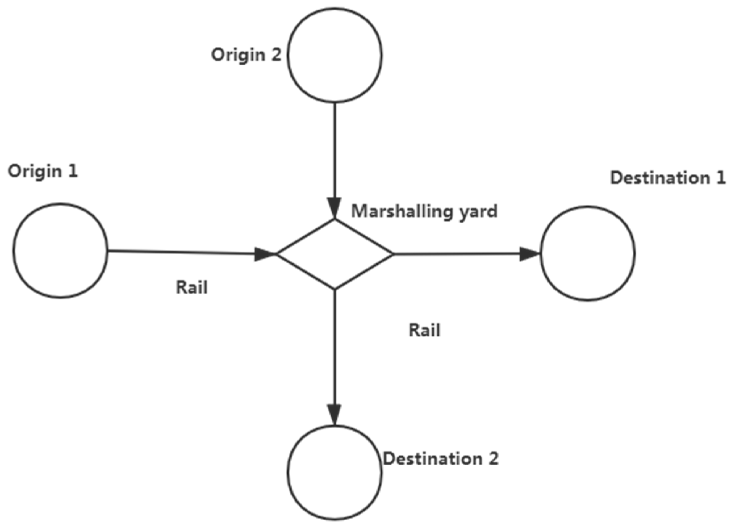
Figure 1. Hazmat railway transportation system of transfer transportation case.
Mathematics 13 00803 g001
Figure 2. Alternative Representations of Case Study Railway Network.
Mathematics 13 00803 g002
Figure 3. Three-dimensional graph of the correlation between R e and route distance/average risk/Hazmat number. (a) Correlation among, average risk and Hazmat number; (b) Correlation among, average risk and route distance; (c) Correlation among, route distance and Hazamat number.
Mathematics 13 00803 g003
Figure 4. CVaR and CVaRE value for the optimal route of two models in problem P. (a) CVaR value for the optimal path varying with α; (b) CVaRE value for the optimal path varying with α.
Mathematics 13 00803 g004aMathematics 13 00803 g004b
Table 1. Optimal route based on CVaR of all O-D pairs and the corresponding value of y.
OriginDestinationN(v)CVaR *Route t : y = c t
1123020,256.98[1, 21, 12]17
135945,842.12[1, 4, 19, 7, 3]23
4143949,434.77[4, 13, 23, 18, 6, 14]9
437434,381.59[4, 19, 7, 3]23
412 5430,385.47[4, 1, 21, 12]
5142327,984.10[5, 22, 6, 14]10
5133530,385.47[5, 21, 1, 13]17
712531,266.28[7, 19, 4, 1]8
7153730,606.14[7, 3, 17, 15]11
9133144,517.62[9, 3, 7, 19, 13]6
1072069,064.39[10, 16, 8, 3, 7]1
11142446,753.52[11, 4, 13, 23, 18, 6, 14]1
131038129,906.74[13, 19, 7, 3, 8, 16, 10]23
1535418,733.65[15, 17, 3]11
1592726,859.05[15, 17, 3, 9]6
15194045,842.12[15, 17, 3, 7, 19]23
1621102186,583.81[16, 8, 3, 7, 19, 4, 1, 21]25
161354115,262.50[16, 8, 3, 7, 19, 13]23
162330100,118.54[16, 8, 3, 7, 19, 13, 23]9
1693164,910.37[16, 8, 3, 9]6
17163672,276.81[17, 3, 8, 16]11
18204843,250.94[18, 6, 20]28
181637112,363.00[18, 6, 14, 24, 16]21
20113038,540.30[20, 2, 13, 4, 11]1
2051836,919.47[20, 6, 22, 5]3
22241225,710.35[22, 6, 14, 24]1
22162996,069.21[22, 6, 14, 24, 16]10
24103978,724.22[24, 16, 10]32
31252117,998.97[3, 7, 19, 4, 1, 21, 12]23
* indicates the optimal value.
Table 2. The relationship between Risk equity ( R e ) and other variables of different O-D pairs.
O-D PairN(v)Distance (P) R e R ¯ ( × 10 4 )
(1, 12)3037416,906.0325.36
(1, 3)59553034.35
(4, 14)3955015,532.2515.20
(5, 13)3558136,197.4615.85
(9, 13)3158714,621.1318.92
(10, 7)202747886.0615.21
(11, 14)246068364.418.39
(13, 10)385861880.5640.45
(16, 13)54544063.04
(16, 21)10287814,254.9099.60
(16, 23)3064520,646.3622.06
(18, 16)3770915,214.8031.11
(22, 16)2910022822.429.48
(24, 10)3917632,237.5761.71
(3, 12)5292734,307.5434.83
Table 3. Comparison of VaR, CVaR, and CVaRE Models, when O-D is 18-16, N(v) = 37.
ModelConfidence Level
α
Risk-Measure ValueRoute Properties
CVaRE *CVaR *VaR *Number of ArcsDistance (km)
CVaR00.01890.012404303
0.99999989158,818.48106,068.9910,755.564303
0.99999990170,387.44112,363.0010,807.084303
0.99999995190,079.78159,650.1711,460.537709
0.99999997250,355.35199,639.3517,737.437709
0.99999999804,905.68118,086.3339,362.113297
CVaRE00.01890.012404303
0.99999989129,759.72115,928.0810,755.567709
0.99999990135,202.78119,987.9810,807.087709
0.99999995190,079.78159,650.1711,460.537709
0.99999997250,355.35199,639.3517,737.437709
0.99999999427,682.78275,534.7739,362.117709
* indicates the optimal value.
Table 4. Sum optimal result of CVaR, CvaRE (different cases), and cost.
C V a R C V a R E Cost (CNY)
Direct transportation(base case)1,721,712.712,234,020.542,349,421.56
Transfer transportation1,848,079.102,777,571.412,361,436.20
Min cost (P)1,906,528.873,014,526.372,169,930.12
Disclaimer/Publisher’s Note: The statements, opinions and data contained in all publications are solely those of the individual author(s) and contributor(s) and not of MDPI and/or the editor(s). MDPI and/or the editor(s) disclaim responsibility for any injury to people or property resulting from any ideas, methods, instructions or products referred to in the content.