Abstract
The generalized linear autoregressive moving-average model (GLARMA) has been used in epidemiology to evaluate the impact of pollutants on health. These effects are quantified through the relative risk (RR) measure, which inference can be based on the asymptotic properties of the maximum likelihood estimator. However, for small series, this can be troublesome. This work studies different types of bootstrap confidence intervals (CIs) for the RR. The simulation study revealed that the model parameter related to the data’s autocorrelation could influence the intervals’ coverage. Problems could arise when covariates present an autocorrelation structure. To solve this, using the vector autoregressive (VAR) filter in the covariates is suggested.
Keywords:
time series of counts; INAR models; integer-valued data; respiratory diseases; air pollution MSC:
62M10
1. Introduction
Time series of counts are non-Gaussian processes composed of non-negative integers. These series can be found in different scientific areas, such as economics, medicine, agriculture, social and physical sciences, and sports. Some examples are the daily number of hospital admissions for a disease, the number of car accidents in a region, and the number of transactions of a given stock observed in one minute. In recent decades, various approaches have emerged to model correlated count series. Recently, ref. [] presented a review of these methodologies and discussed recent developments on this topic.
The impact of air pollution on population health has been the subject of many studies in the last decades; see [,,,], among others. The massive and continuous development of cities and communities leads to urbanization and industrialization. However, it can cause environmental and health problems as many activities generate residues that affect inhabitants’ quality of life [].
Epidemiological studies have consistently provided evidence of the association between daily levels of pollutant concentration and hospital admissions, morbidity, and mortality, mainly caused by respiratory and cardiovascular diseases; see [,] for references. Epidemiological data are frequently treated as time series of counts because they record the relative frequency of certain events in successive time intervals. In this context, many authors have been using the generalized additive model (GAM) [] with Poisson marginal distribution to quantify the association between the effects of air pollution on health.
Alternative methods such as wavelet transforms have shown promise in capturing complex temporal patterns in time series, particularly those with non-stationary behavior or cyclical components, such as air pollution data. Ref. [] demonstrated the application of wavelet transforms combined with a weighting forecasting model to predict air pollution levels, highlighting their robustness in handling complex environmental data sets. Furthermore, last-squares wavelet analysis (LSWA), as described in [], offers a robust framework for time-frequency analysis, even with high noise levels and missing data. LSWA has been successfully applied to simulated time series for component estimation at various confidence intervals and forecasting purposes, demonstrating its versatility and reliability.
Despite widespread use, care is required when applying the GAM to time series. The GAM assumes that errors are mutually independent and, therefore, cannot capture the time-dependent structure of the observations. One way to circumvent this is to use the generalized linear autoregressive moving-average (GLARMA) model, proposed by [], which adds an ARMA structure to generalized linear models (GLMs) []. The GLM is an extension of the Gaussian linear model, where the distribution of the response variable belongs to the exponential family.
The GLARMA model allows for modeling correlated observations from the exponential family. Despite its complexity in estimating general models, this methodology has been widely applied in various fields (see, e.g., [,,,,,], among others). As discussed by [], the GLARMA family is one of the most flexible and easily adaptable count models, effectively balancing parameter-driven and observation-driven approaches. Besides the GLARMA model, different approaches to modeling count time series were also suggested in the literature. Ref. [] proposed a quasi-likelihood approach to time series regression, which was generalized by [] and called generalized autoregressive moving-average models (GARMA).
Ref. [] proposed the Autoregressive Conditional Poisson model (ACP), able to model overdispersion, and ref. [] proposed log-linear models for time series. Recently, ref. [] proposed a model using the GAM with autoregressive moving-average terms (GAM-ARMA). This procedure can model the temporal correlation structure and estimate nonlinear associations between the covariates and the response variable. Following the Bayesian approach, ref. [] used state-space models with conjugate prior distributions, where the counts are modeled as a Poisson distribution, and ref. [] proposed a family of non-Gaussian state-space models.
In epidemiology, the relative risk (RR) is a standard statistical measure used to quantify the relationship between contaminant levels and adverse health effects. Beyond point estimation, epidemiologists are also interested in interval estimation for RR. Although the asymptotic properties of the maximum likelihood estimators are not yet established for the general case in GLARMA models, confidence intervals (CIs) for relative risks are often computed under normality assumptions. While this approach is not problematic for large sample sizes, it may be unreliable for small samples.
Still underexplored in studies related to air quality, bootstrap CIs can be calculated without any assumptions about data distribution. This procedure, introduced by [] initially for independent observations, has been extended to more general situations. Refs. [,,] used a classic model-based approach, where bootstrap samples are generated using the estimated model structure and independently and identically distributed (i.i.d.) sampling residues. Ref. [] used the classical idea of the residual-based bootstrap for semiparametric generalized models. Ref. [] proposed a nonparametric bootstrap for the stationary process, the blockwise bootstrap, where blocks of consecutive observations are resampled. This method is robust against misspecification models, but the block dependence is neglected. Ref. [] proposed another nonparametric methodology, the sieve bootstrap, an approach to real-valued time series where an autoregressive process of order p, AR(p), is adjusted to the observations to approximate the real data distribution. In this procedure, the bootstrap samples are obtained by resampling from the centered residuals of the autoregressive process fitted. Due to the popularity of the sieve bootstrap and its simple implementation, in recent years, many authors have proposed methodologies to adapt it to time series of counts. The most simple and probably obvious approximation is to centralize the counts and adjust the AR(p) process to the centralized observations. However, this approach leads to valid bootstrap approximation only for a limited number of cases (for details, see []).
In the last decades, the most prominent works proposing approaches for the sieve bootstrap considered the integer-valued autoregressive (INAR) time series, motivated by the fact that the AR and INAR processes share the same autocorrelation function. In the INAR model, the dependent count observation, , is expressed as a function of the p preceding values plus an innovation , with , where G is a distribution with range . Refs. [,,] proposed relevant alternatives to constructing appropriate confidence intervals’ bootstrap for the INAR models. Ref. [] proposed an efficient method for bootstrapping INAR models. This paper addressed a critical literature review, highlighting the bootstrapping count time series challenge and the limitations of the proposed techniques considering INAR models. Ref. [] introduced a general INAR-type procedure, where the INAR(p) model is adjusted to the count time series and a marginal distribution is attributed to the bootstrap innovations. The authors proved the consistency of this procedure, assuming parametric and nonparametric distributions for the bootstrap innovations. In addition, they investigated the performance of this procedure by analyzing the coverage of CIs for diverse statistics based on the observations. Their numerical simulation illustrates the superiority of the proposed method over the blockwise, sieve, and Markov bootstraps.
Based on the above discussion and the real data problem, this paper compares and evaluates different bootstrap approaches for computing confidence intervals for relative risk using GLARMA models, focusing on their coverage rates. For this, three of those techniques cited previously were examined: the classic model-based approach, based on the work of [], the well-known sieve bootstrap, and the INAR-type bootstrap. Confidence intervals assuming Gaussian distribution for the estimators were also calculated.
Although the authors of [] have already verified the superiority of their methodology over the sieve bootstrap for statistics based on the dependent count observations, here we aim to compare the performance of the investigated methods applied to the GLARMA model. An extensive simulation study was performed considering distinct sample sizes, types of covariates, and different autocorrelation structures for a response variable autocorrelated and conditioned to the past, following a Poisson distribution. The objective was to verify if any change in the characteristics of the model’s covariates or the complexity of the autocorrelation structure in the GLARMA model could impact the coverage or amplitude of the calculated intervals.
A real-time series was analyzed to illustrate the findings of the numerical simulations. We computed confidence intervals for the RR to quantify the impact of air pollutants on the number of chronic obstructive pulmonary disease cases in the metropolitan area of Belo Horizonte, Brazil. This study addresses a critical gap in the literature, as few works have explored bootstrap methods with GLARMA models in the context of relative risk estimation. Moreover, the motivation stems from the practical importance of accurately quantifying uncertainty in real-world time series data, such as those related to public health or environmental studies, where reliable interval estimates are crucial for decision making.
This paper is organized as follows. Section 2 presents the GLARMA model and some essential properties regarding the model and the parameter estimation. Section 3 discusses the bootstrap for time series of counts, where three approaches are introduced. Simulation studies are performed in Section 4, considering different scenarios and sample sizes. A real data analysis is carried out in Section 3.2, and Section 4 presents the final considerations of the work.
2. Methodology
2.1. The Generalized Linear Autoregressive Moving-Average Model
The GLARMA models are a class of observation-driven state-space models. The state process consists of linear regression and observation-driven components comprising an autoregressive moving-average filter of past predictive residuals.
Let be the observations and , where is the past of the counting process and is the past and present of the regressor variables. Conditional on , the observations are independent and have a distribution in the exponential family with density
where and are known real functions and summarizes the information in ; see [,].
Ref. [] considered that the specification of in (1) is given by
where is the vector of covariates of dimension , is a () × 1 vector of unknown coefficients to be estimated, and the standard residuals are defined as
for .
The infinite moving-average weights in (2) can be specified in terms of an autoregressive moving-average (ARMA) filter:
where the autoregressive and moving-average components and are polynomials with roots outside the unit circle, is the parameter vector formed by s and s, and B is the backshift operator of the form . Defining , where , for and and for , the process is computed according to the following ARMA-like recursions:
Remark 1.
Let and for . Under these conditions, it is easy to show that the form a martingale difference sequence with zero mean, variance given by , and for . In addition, for any , , and, for , . For more details, see Section 2.2 in [].
Remark 2.
For , ref. [] showed that considering the simplest model, where and , assuming and , the process has a unique stationary distribution and is uniformly ergodic. For , is bounded in probability and therefore has a stationary distribution, yet the uniqueness of this distribution is currently unknown.
Define as the parameter vector of the model (2). Let be a sample from the process ; the log-likelihood of conditional to is given by
For the exponential family, the log-likelihood becomes
As a particular case, for , where , the log-likelihood is given by
The log-likelihood function can be maximized using Newton–Raphson iteration and Fisher scoring approximation procedures. Defining the first and second derivatives of the log-likelihood by and , we have
and
At the true parameter of , , the expected value of the first summation in (9) is zero, which motivates the Fisher scoring approximation:
Note that ; however, these expectations cannot be calculated in closed form. Thus, the Newton–Raphson (using ) and the Fisher scoring (using ) methods are used to maximize the log-likelihood function.
Ref. [] discussed that the consistency and asymptotic properties of the maximum likelihood estimator were proven only for the simplest model cited in Remark 2. For this special case, stationarity and ergodicity were established rigorously. In general, for inference purposes, it is assumed that the central limit theorem holds.
In the epidemiology context, the impact of air pollutants on human health is evaluated by relative risk (RR). The RR of a variable is the change in the expected count of the response variable per -unit change in the , keeping the other covariates fixed. The authors of [] present its mathematical representation:
For Poisson regression, the RR is given by
and its approximate confidence interval (CI) at an significance level in the GLARMA with a Poisson marginal distribution is
where is the conditional maximum likelihood estimator of , se is the estimated standard deviation of , and denotes the -quantile of the standard normal distribution.
2.2. Bootstrap for Count Time Series
Initially proposed by [] for independent variables, the bootstrap is a resampling method that attributes measures of accuracy to statistical estimates. It is a computer-based procedure that approximates the theoretical distribution by the empirical distribution of a finite sample of observations.
Let and denote the random sample and its observed realizations, respectively, from a distribution F. A bootstrap sample is obtained by randomly sampling n times, with replacement, from the original data points . That is, the bootstrap sample is drawn from the empirical distribution . For any statistic u computed from the original sample data, it is possible to define a statistic by the same formula but calculate it using the resampled data.
Ignoring the temporal correlation of the time series can impact the estimations. In this context, many approaches have been proposed, standing out from the classic model-based [,,], the blockwise [], and the sieve [] bootstraps. In the residual model-based approach, the bootstrap replications are based on i.i.d. resampling of residuals. The blockwise and sieve bootstraps are nonparametric procedures that are robust against model misspecification, as discussed in []. In the first case, blocks of consecutive observations are resampled. In the sieve bootstrap, the autoregressive process of order p, AR(p), is adjusted to the observations to approximate the actual data distribution.
However, the challenge arises when the bootstrap is applied to non-Gaussian responses. Several authors have studied the bootstrap involving time series of counts in recent decades. Ref. [] proposed a methodology derived from the classic model based on semiparametric generalized models. Refs. [,,,] proposed approaches to adapt the sieve bootstrap considering integer-valued autoregressive (INAR) time series.
In this section, three bootstrap procedures for count time series are discussed: the residual model-based approach of [], an adaptation of the sieve bootstrap for count observations, and the proposal of [] for the INAR(p) process.
2.2.1. Classic Model-Based Bootstrap
This procedure is used in regression problems, in which it is assumed that the model is correctly specified and the error terms in the model are independent and identically distributed. The basic idea of the bootstrap with parametric assumptions is to obtain residuals using the estimated parametric model and then generate bootstrap samples using the estimated model structure and i.i.d. resampling of residuals. Assume that , given the past history, , has a distribution in the exponential family with , , where g is a known link function and the component is defined in Equation (5). The bootstrap procedure works as follows:
- (1)
- Compute the residuals .
- (2)
- Resample the estimated residuals with replacements generating the bootstrap residual samples .
- (3)
- Generate bootstrap observations according to
In Algorithm 1, we present the procedure for calculating the parametric bootstrap for regression models, referred to here as the classic model-based bootstrap:
| Algorithm 1 Parametric Bootstrap Procedure for Regression Models |
|
This procedure is model-based, and misspecification problems can be observed, e.g., biased parameters and inconsistent standard errors. The sieve bootstrap, presented below, follows the same strategy of fitting a parametric model and resampling the residuals but approximating an infinite-dimensional nonparametric model by a sequence of finite-dimensional parametric models.
2.2.2. Sieve Bootstrap
Let be a real-valued stationary process, and denote a sample from this process. The basic idea of the sieve bootstrap [] is to adjust an autoregressive process of order p to the data:
with increasing order p as the sample size n increases. The estimated coefficients are then used to compute the residuals . These residuals are centered, , and the bootstrap sample is constructed according to the recursion
where is a random sample with replacement of the centered residuals.
The sieve bootstrap was initially proposed for real-valued data, but a simple approximation can be performed by ignoring the discrete nature of the process. Ref. [] cited this approach as follows:
- (1)
- Compute the centered observations , where .
- (2)
- Fit an AR(p) to the centered datawhere the estimated AR coefficients can be obtained, e.g., from Yule–Walker estimates.
- (3)
- Compute the estimated residuals , and center them obtaining as presented previously.
- (4)
- Generate bootstrap observations according towhere randomly and uniformly resamples from the centered residuals.
- (5)
- The AR bootstrap sample of the original process can be calculated as .
Ref. [] showed that the sieve bootstrap captures the autocovariance structure of a process and will always be consistent for the sample mean and any statistic that depends exclusively on the autocovariance structure of the process under mild conditions. Algorithm 2 presents the procedure for calculating the sieve bootstrap:
2.2.3. INAR-Type Bootstrap
Ref. [] proposed the procedure based on the INAR model introduced by [,] and extended by [,].
The integer-valued autoregressive process of order p, denoted by INAR(p), expresses the value of the variable of interest at time t as a function of the p preceding values and an innovation in the following way:
where is a sequence of non-negative integer-valued variables, is an i.i.d non-negative integer-valued random variable with finite mean and variance , and , such that . The operator “∘” in (15) is called the and , where denotes the binomial distribution with parameters n and . Due to the random thinning operator, the INAR models are nonlinear, contrary to the sieve bootstrap, which belongs to the linear time series process class. It is important to observe that the INAR innovations and the sieve errors were distinguished here. As these procedures share the same autocorrelation function, the INAR coefficients can be estimated using techniques from classical time series analysis such as Yule–Walker, Least-Squares, or Maximum-Likelihood estimators. The authors of [] proved that if the autocorrelation of an INAR(p) process corresponds to that of an autoregressive process of order p, AR(p). However, unlike the sieve bootstrap, the procedure proposed by [] does not explicitly use the residuals from the fitted model. Let be a non-negative integer-valued time series. The general INAR bootstrap scheme is defined as follows:
- (1)
- Fit an INAR(p) process as in Equation (15) to obtain the estimates of for the INAR coefficients;
- (2)
- Specify the marginal distribution for the innovations ;
- (3)
- Generate the bootstrap samples according towhere denotes the mutually independent bootstrap binomial thinning operations and () are i.i.d. random variables following the distribution .
| Algorithm 2 Sieve Bootstrap for Time Series Data ([]) |
|
The estimation of the parameters and the choice of the distribution , in steps 1 and 2, respectively, can be calculated following parametric and semiparametric approaches. Here, the parametric perspective was considered. In this case, under some assumptions related to the marginal distribution G of the innovation process (see []), the bootstrap innovations can be easily generated from following the steps above. In Algorithm 3, we present the procedure for calculating the bootstrap INAR(1):
| Algorithm 3 Bootstrap INAR(1)—([]) |
|
2.2.4. Bootstrap Confidence Intervals
Bootstrap confidence intervals can be computed using simple percentiles, bias-corrected percentile limits, bias-corrected and accelerated percentiles (BCa), and the Student’s t method, among other proposals. Here, we will focus on the approach used by [] in their simulations. To compute the bootstrap confidence interval for a parameter , these authors first calculated a centering measure cent() and the centered bootstrap estimates cent. Then, the bootstrap confidence interval was calculated using the ()- and -quantiles from as follows:
where is the estimate obtained from the sample.
As the main objective of this paper is to calculate bootstrap confidence intervals for the RR of the variable , the CIs were constructed as follows:
where is the i-th estimated coefficient, is the bootstrap estimate, and , with being the mean of . The interquartile variation of is given by , and is the significance level.
In Algorithm 4, we present the procedure for calculating the bootstrap confidence intervals for the RR:
| Algorithm 4 Bootstrap Confidence Interval for the Relative Risk (RR) |
|
3. Results
3.1. Simulation Study
A simulation study was conducted to evaluate and compare the performance of the bootstrap approaches presented in Section 2.2. As many studies use asymptotic confidence intervals for the RR based on the Gaussian distribution, this interval was also considered for comparison purposes. This analysis focused on the confidence intervals for the relative risk calculated from the GLARMA(1,0) Poisson model, given by
where is given by
In this simulation study, we analyze time series data representing pollutant levels, such as carbon monoxide (CO), as input variables. The pollutant values, denoted as , are combined with fixed parameters ( and ) to generate the response variable , which reflects health outcomes. We model this relationship using a GLARMA(1,0) Poisson model.
In the data-generating process, the initial value for was set as the mean of the response variable Y, while was set to zero. Regarding the burn-in period, in our implementation, we discarded the first 30% of the generated iterations to ensure that the sampled values more accurately reflected the stationary properties of the process.
The output data consist of bootstrap samples of the estimated parameters generated using the procedures outlined in Section 2. These bootstrap samples are subsequently used to compute confidence intervals for the relative risk (RR). Figure 1 provides a general illustration of this procedure.
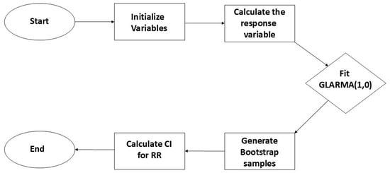
Figure 1.
Flowchart of simulation study.
The effectiveness of the bootstrapping method for non-Gaussian distributions depends on the sample size, as the central limit theorem ensures a better approximation of the sampling distribution as the sample size increases ([], p. 153). Although no universally defined minimum sample size exists, previous studies suggest that samples with at least 30 to 50 observations are often sufficient for reasonable estimates.
3.1.1. Large Samples
For this simulation study, three scenarios were considered:
- S1: and , where .
- S2: and , where is an independent random vector in time and .
- S3: and , where , with the autoregressive parameter assuming values 0.2, 0.5, and 0.8.
These scenarios were selected with specific objectives: Scenario 1 uses the covariate from [] for comparison purposes. Scenario 2 considers a covariate with no temporal dependence, allowing us to examine the impact of the absence of a temporal structure on the bootstrap intervals. Scenario 3 incorporates a covariate with distinct levels of temporal dependence, aiming to assess the influence of more complex temporal structures on the variables. Of the three scenarios, Scenario 3 is the most closely related to real-world situations, as pollutants typically exhibit temporal dependence.
The considered sample size n was equal to 1000. The values of in Equation (19) were fixed at 0.2, 0.4, and 0.6, and the nominal level for the confidence intervals was fixed at 95%. The parameter assumed the value 1.0. Although [] showed that, for , only in the simplest model, the process has a stationary and ergodic distribution, the numerical simulations revealed that, even for complex models, this value of provides better estimates. For all scenarios, the parameter values used in the simulations were chosen for simplicity, with . Additional simulations conducted with different values of produced similar results, indicating that the findings are not sensitive to the specific choice of parameter values.
The classic model-based bootstrap considers the three steps presented in Section 2.2.1 to construct the confidence intervals. For the sieve and INAR(1) cases, the steps shown in Section 2.2.2 and Section 2.2.3 were applied to the count time series , and then the GLARMA Poisson model was fitted considering the bootstrap samples as the response variables. In addition, for the INAR(1) bootstrap, an INAR process having Poisson-distributed innovations was assumed with and , where was obtained by Yule–Walker estimation.
The Monte Carlo simulations were repeated 500 times with 500 bootstrap replications. The asymptotic confidence interval was estimated as in Equation (12). All the codes were written in the R language and are available from the authors upon request.
- Scenario 1
Table 1(a) presents the mean and standard deviation of the 500 Monte Carlo estimates of parameters , , and in scenario 1 (S1). For and parameters, the mean of the estimates was close to the real values, especially when or . Conversely, the standard deviation shows a consistent increase with the value of . Parameter is better estimated for small values. Table 1(b) presents the 95% confidence intervals for the RR of the covariate . The values in square brackets are the calculated intervals’ average lower and upper limits. The results indicate that classic and sieve bootstrap methods exhibit a decline in coverage as increases. Specifically, for the classic bootstrap, the coverage drops from 0.884 to 0.729, while for the sieve bootstrap, the decrease is even more pronounced, from 0.927 to 0.570. Notably, for , the sieve bootstrap still achieves a coverage rate close to the nominal level of 0.95, suggesting that it may be a reasonable choice in this scenario. However, for higher values of the autoregressive parameter, both methods present considerably lower coverage, indicating potential limitations in their performance under strong dependence. In contrast, the INAR(1) bootstrap and the asymptotic confidence intervals maintained a coverage rate of approximately 95% for all values of .

Table 1.
(a) The mean and standard deviation of the Monte Carlo estimates of parameters , , and in scenario 1 (S1). (b) The coverage and the average lower and upper limits of the 95% confidence intervals for the RR = exp() (S1).
Scenario 1 studied the impact of the same covariate considered in [], although the authors only evaluated cases where the time correlation is a moving-average process of order 1. Real data sets commonly present an autoregressive autocorrelation structure. In this case, S1 showed that even when the time correlation structure is complex (e.g., ), for deterministic covariates (), the asymptotic theory and the INAR(1) bootstrap presented coverage rates close to the nominal level of the confidence intervals.
- Scenario 2
In the parameter estimation presented in Table 2(a), the mean of the estimates was close to the real values of all parameters, except when . It can also be seen that the standard deviations were much affected by the increase in . Table 2(b) presents the 95% confidence intervals for the RR in scenario 2 regarding the covariate . Table 2(b) shows that for the classic bootstrap, the coverage rate was close to 1 for all values of , which means that almost 100% of the intervals contain the true relative risk value. Regarding the sieve bootstrap, for and , the coverage rate was also close to 1. Meanwhile, for , the coverage rate decreased to 0.849. The INAR(1) bootstrap and the asymptotic intervals had similar performance, with coverages close to 0.95 for and and considerably below the nominal level for . It should be pointed out that the INAR(1) bootstrap always presented coverages closer to 0.95 than the asymptotic interval, even for the case.
Table 2.
(a) The mean and standard deviation of the Monte Carlo estimates of parameters , , and in scenario 2 (S2). (b) The coverage and the average lower and upper limits of the 95% confidence intervals for the RR = exp() (S2).
Scenarios 1 and 2 showed that the coverage of the INAR bootstrap and asymptotic approaches were close to the nominal level for and , where was appropriately estimated. In Table 1(a) and Table 2(a), the mean of this parameter is close to the true values, and although the standard deviation goes up in Table 2(a), the coverage in scenario 2 is not impacted. However, for , the estimates were terrible, mainly in S2, and as the RR depends on , the interval coverage was also impacted. Finally, it is essential to observe that the coverage intervals are unsuitable for classic and sieve bootstraps even when the estimates are reasonable.
- Scenario 3
In epidemiology, it is common for air pollutants to present temporal correlation. To simulate this behavior, in scenario 3, the covariate followed an autoregressive process of order 1:
where is an AR(1) process with autoregressive parameter and is defined by Equation (5). To evaluate the time structure’s impact, the covariate’s autoregressive parameter () assumed values equal , and . Table 3(a) presents the parameter estimates for all values of . For , when focusing on , the mean estimate of this parameter is close to the true value for , while the estimate becomes less accurate for and , accompanied by an increase in the standard deviation.
Table 3.
(a) The mean and standard deviation of the Monte Carlo estimates of parameters , , and in scenario 3 (S3). (b) The coverage and the average lower and upper limits of the 95% confidence intervals for the RR = exp() (S3).
In the case of , shown in Table 3(a), the mean of the estimate remains close to the true value for . However, compared to the results for the exact value of in Table 3(a), there is a noticeable increase in the standard deviation. For both and , the estimates deteriorate, and the standard deviation increases as the value of rises.
Table 3(a) also shows the parameter estimates when the covariate’s autoregressive parameter () is . Even for the smallest value of considered, the mean estimate of is poor, and the standard deviation is significantly high. For and , the means of the estimates become much worse, and the standard deviation increases even further.
Table 3(b) presents the 95% confidence intervals (CIs) for the relative risk (RR) of the covariate . For , the coverage rate for the classic model-based bootstrap was close to 1 for all values of . The performance of the asymptotic approach, sieve bootstrap, and INAR(1) bootstrap was similar, with the coverage decreasing for . For , all methods exhibited poor performance.
For , as shown in Table 3(b), a similar performance was observed for the classic and sieve bootstraps, with the coverage rate equal to 100% for , followed by a drop in coverage as increased. Both methods also produced large confidence intervals. The coverage rate of the INAR(1) and asymptotic approaches was approximately 95% for . For , these rates decreased, with the INAR(1) bootstrap maintaining the highest coverage. Again, for , all methods showed substantial deviations from the nominal coverage level.
For , Table 3(b) shows that for , the classic model-based and sieve bootstraps had coverage rates close to 1, while the INAR(1) bootstrap and asymptotic approach exhibited coverage rates of 0.93 and 0.895, respectively. For and , all methods saw a significant decline in the coverage rate, with the CIs from the asymptotic approach and INAR(1) bootstrap being the most affected.
In general, we observed that the INAR method appears to perform better, alongside the asymptotic method, as they present narrower confidence intervals and coverage rates closer to the nominal value. On the other hand, the classic and sieve methods showed very poor coverage in some cases, with coverage rates close to 1, while the nominal value was 0.95. This suggests that the INAR and asymptotic approaches are more reliable for estimating the relative risk in scenario 3, although the coverage rate was in general inferior than that observed in scenario 2.
The comparison between scenarios 2 and 3 indicates that time correlation in the covariates can impact the coverage rate of the confidence intervals; as the autoregressive structure becomes more complex, the interval coverage becomes smaller. Table 3(a) showed that the values of strongly impact the parameter estimation, and this effect becomes worse as this autoregressive parameter increases in the direction of the nonstationarity region, either in the covariate or in the component. It is easy to verify that for any , , where the covariate is an independent random vector in time. However, for AR(1), the variability of the state process increases, which inflates the model estimates, directly impacting the coverage rates of the RR.
Beyond the empirical investigations discussed here, scenarios with more complex model structures, such as bivariate time series, were also considered. As expected, the coverage rate was unsatisfactory. Therefore, the authors recommend applying the procedure proposed by [] before implementing the bootstrap approaches discussed in this study in practical situations where covariates are time series. This is further explored in Section 3.2, within the real data analysis, where the covariates follow a vector of time series data.
3.1.2. Small Samples and ARMA Covariate
This work also studied another scenario considering small samples for the GLARMA(1,0) Poisson model. In this case, the sample size was equal to 50, and the single covariate was an ARMA() process:
where is an ARMA process with autoregressive and moving-average parameters and and is defined by Equation (19). Three different ARMA processes were considered. They were chosen due to their temporal structure, which is similar to some atmospheric pollutants in real data:
- (1) , where and .
- (2) , where and .
- (3) , where , , and .
Table 4 presents the 95% confidence intervals for the RR, where , where and . Here, only the INAR(1) bootstrap and the asymptotic approach are compared, as these methodologies presented similar results in the previous simulation studies. The autoregressive parameter was fixed at 0.2 once the simulations presented the best adjustments at this value. In all cases, the INAR(1) bootstrap presented a coverage rate approximately equal to 0.95, while for the asymptotic approach, this rate was close to 0.90.
Table 4.
The coverage rate of the 95% confidence intervals for the RR (n = 50).
The INAR(1) bootstrap presented better results related to the coverage rate for the RR than the asymptotic approach, considering the ARMA process as a covariate. This analysis is relevant in real data sets. The sample size is generally insignificant, and the air pollutants present complex structures, e.g., time correlation, high volatility, and peaks. In addition, the coverage rates were close to 0.95 in the INAR(1) bootstrap even for high values of the autoregressive parameter (), different from those observed in the simulations of scenario 3 (S3), in Section 4.1, where the covariate was an AR(1) process.
3.2. Real Data Analysis
A real data analysis was proposed to study the impact of air pollutants on the monthly number of chronic obstructive lung disease (COPD) cases in Belo Horizonte, Brazil, between 2007 and 2013 (). Figure 2 presents the pollutants considered: Particulate Matter (), Nitrogen Monoxide (), Nitrogen Dioxide (), Carbon Monoxide (), and Ozone (). This figure shows an increasing trend in COPD cases, along with seasonality that may be semiannual and/or annual. The air pollutants show a generally constant trend, with occasional aberrant values. Ozone () appears to exhibit a more pronounced seasonality.
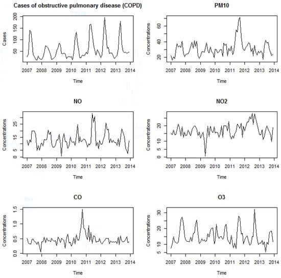
Figure 2.
The time series of the number of COPD cases and concentrations of air pollutants in the metropolitan area of Belo Horizonte, Brazil.
Many covariates can lead to identification problems, and their correlation may imply multicollinearity. A significant correlation among some air pollutants was observed, while and presented the highest correlation with the response variable (COPD). Table 5 presents the correlation matrix among air pollutants and the number of chronic obstructive pulmonary cases. Principal component analysis (PCA) is a possible solution to this problem. This methodology explains a random vector’s variance and covariance structure through linear combinations of the original variables ([]). These combinations, called principal components (PCs), are not correlated with each other. The PCA methodology requires independent observations; however, according to [], if the covariates present a time correlation, then the PCs are also autocorrelated. Based on this, the works of [,] proposed a hybrid model called GAM-PCA-VAR, where the time dependency of data is removed through the VAR process. The PCs are derived from the residuals of VAR, and the GAM model is adjusted with PCs as explanatory variables.
Table 5.
Pearson correlation among pollutants and chronic obstructive pulmonary disease cases.
This study estimated the impact of air pollutants on the occurrence of COPD using the previously mentioned procedure. To model this relationship, it is essential to apply methods that account for the time dependence inherent to COPD cases. The GLARMA model is an attractive option due to its flexibility and easy fit using statistical packages (see []). The time correlation structure of the contaminants was removed by applying the VAR filter, and the PCs were derived from the residuals of VAR. The GLARMA model was fitted using the PCs as covariates. All the principal components were considered, although the first three correspond to almost of the entire structure of variability. The GLARMA Poisson model was adjusted as follows:
where
The annual and semiannual seasonality in the response variable was incorporated into the model with sine and cosine functions. The modeling also included the trend present in the data. This component was modeled using a linear function of time, where a variable ranging from 1 to n was included to account for potential long-term patterns in the data.
Table 6 presents the estimates of the adjusted model, with the corresponding standard errors. We considered different autocorrelation structures and used the AIC and BIC measures to compare them. The best fit was obtained regarding the autoregressive parameter of order 2. All coefficients were significant at the 5% level of significance.
Table 6.
The parameter estimates of a GLARMA(2,0) model fitted to the COPD cases.
Confidence intervals for the relative risk of air pollutants were calculated under the assumption of normality (asymptotic) and using the INAR(1) bootstrap. The RR was computed based on the combination of the PCs. For more details about this estimation, see [], Section 2.2.4. Algorithm 5 outlines the procedure for computing bootstrap confidence intervals.
In the application, we utilized a bootstrap procedure with 1000 iterations to ensure reliable and stable estimates, incorporating a burn-in period set to 30% of the total iterations. This was performed to allow the model to reach a stable state, particularly considering the strong temporal dependence in the data. By discarding the first 300 iterations, we minimized the potential influence of initial conditions on the parameter estimates, ensuring that the results reflected the true underlying process. This approach is especially crucial when the observed values of the series are significantly larger than zero, as in our application.
| Algorithm 5 Bootstrap Confidence Interval Calculations for Pollutant Effects |
|
Table 7 shows that the 95% CIs calculated using asymptotic and bootstrap techniques were similar, corresponding to the conclusions obtained in the simulation study. This real data analysis is equivalent to scenario 2, once the PCA covariates originated from the VAR process are not autocorrelated. For the parameter , the numerical study in Section 3.1.1 revealed that the confidence intervals provided by INAR bootstrap and the asymptotic approach are quite close (see Table 2(b)).
Table 7.
A comparison of the relative risk and 95% confidence intervals for an interquartile variation of the pollutant concentrations.
4. Discussion
This work proposed to study three bootstrap confidence interval approaches for the relative risk calculated from GLARMA models: the classic model-based approach, a procedure based on the specifications of the model, the sieve bootstrap well known in the literature for real-valued processes, and the recently proposed INAR(1) bootstrap based on the structure of the integer-valued autoregressive process.
An extensive numerical study was performed considering different scenarios and sample sizes. For large samples, the analysis showed that the model parameter () could impact the estimates and, consequently, the coverage rate of the intervals. The primary reason for this behavior may be that, for high values of , the convergence of the maximization method is not guaranteed. Similar behavior has been observed in GLARMA models by [,]. In particular, ref. [] reported that when , the likelihood function struggles to reach the global maximum. This effect became more pronounced as the complexity of the covariate time structure increased.
The observations in this study agree with the conclusions of [,], which demonstrated that removing the temporal structure of covariates prior to modeling improves the accuracy of parameter estimation and confidence interval coverage. In this study, the best results were verified when did not exhibit time correlation, equivalent to the variables filtered by the VAR process. This reinforces the importance of preprocessing time-dependent covariates in regression models.
Moreover, this study aimed to evaluate the performance of different methodologies for estimating confidence intervals in small-sample scenarios, particularly those mimicking real-world complexities in air pollution data. In all cases, the INAR(1) bootstrap outperforms both the classic model-based and sieve bootstrap approaches. Among the methods evaluated, the INAR(1) bootstrap consistently provided confidence intervals with coverage rates closest to the nominal 95% level, whereas the asymptotic approach tended to underestimate variability. This finding aligns with the observations of [], which highlighted that using residuals from Poisson regression models typically underestimates the true serial dependence. Thus, for practical applications involving count time series, the INAR(1) bootstrap presents itself as the most reliable alternative, particularly in small-sample contexts.
In a real data set analysis, we assessed the impact of air pollutants on the monthly number of COPD cases in Belo Horizonte, Brazil. The best-fitting model incorporated an autoregressive structure of order 2, effectively capturing the temporal dependence in the data. All estimated coefficients were statistically significant at the 5% significance level, reinforcing the model’s reliability and highlighting the importance of the selected predictors—specifically, air pollutants, trend, and seasonality components—in explaining the outcome variable.
To evaluate the robustness of our methodology, we compared the confidence intervals obtained via the INAR(1) bootstrap and the asymptotic approach. As observed in the empirical study, both approaches yielded comparable intervals, confirming the consistency of our method in real-world applications. These findings emphasize that, in practice, the INAR(1) bootstrap provides a reliable alternative for modeling relative risk in environmental epidemiology studies, ensuring more accurate inference even in complex data structures.
Author Contributions
Methodology, A.J.A.C., V.A.R. and G.C.F.; Validation, A.J.A.C.; Formal analysis, A.J.A.C.; Data curation, A.J.A.C.; Writing—original draft, A.J.A.C.; Writing—review & editing, V.A.R., G.C.F. and P.B.; Supervision, V.A.R. and P.B.; Funding acquisition, P.B. All authors have read and agreed to the published version of the manuscript.
Funding
The authors thank the Brazilian Federal Agency for the Support and Evaluation of Graduate Education (Coordenação de Aperfeiçoamento de Pessoal de Nível Superior—CAPES), National Council for Scientific and Technological Development (Conselho Nacional de Desenvolvimento Científico e Tecnológico—CNPq), Minas Gerais State Research Foundation (Fundação de Amparo à Pesquisa do Estado de Minas Gerais—FAPEMIG), and Espírito Santo State Research Foundation (Fundação de Amparo à Pesquisa do Espírito Santo—FAPES). This research was also supported by the DATAIA convergence institute as part of the “Programme d’Investissement d’Avenir”, (ANR-17-CONV-0003) operated by CentraleSupélec.
Data Availability Statement
The original contributions presented in this study are included in the article. Further inquiries can be directed to the corresponding author.
Conflicts of Interest
The authors declare no conflicts of interest. The funders had no role in the design of the study; in the collection, analyses, or interpretation of data; in the writing of the manuscript; or in the decision to publish the results.
References
- Davis, R.; Fokianos, K.; Holan, S.; Joe, H. Count time series: A methodological review. J. Am. Stat. Assoc. 2021, 116, 1533–1547. [Google Scholar] [CrossRef]
- Ostro, B.; Eskeland, G.; Sánchez, J.; Feyzioglu, T. Air pollution and health effects: A study of medical visits among children in Santiago, Chile. Environ. Health Perspect. 1999, 107, 69–73. [Google Scholar] [CrossRef] [PubMed]
- Schwartz, J. Harvesting and long-term exposure effects in the relationship between air pollution and mortality. Am. J. Epidemiolology 2000, 151, 440–448. [Google Scholar] [CrossRef]
- Chen, R.; Chu, C.; Tan, J.; Cao, J.; Song, W.; Xu, X.; Jiang, C.; Ma, W.; Yang, C.; Chen, B.; et al. Ambient air pollution and hospital admission in Shanghai, China. J. Hazard. Mater. 2010, 181, 234–240. [Google Scholar] [CrossRef]
- Borhan, S.; Motevalian, P.; Ultman, J.; Bascom, R.; Borhan, A. A patient-specific model of reactive air pollutant uptake in proximal airways of the lung: Effect of tracheal deviation. Appl. Math. Model. 2021, 91, 52–73. [Google Scholar] [CrossRef]
- Barbera, E.; Currò, C.; Valenti, G. A hyperbolic model for the effects of urbanization on air pollution. Appl. Math. Model. 2010, 34, 2192–2202. [Google Scholar] [CrossRef]
- Souza, J.; Reisen, V.; Franco, G.; Ispány, M.; Bondon, P.; Santos, J. Generalized additive models with principal component analysis: An application to time series of respiratory disease and air pollution data. J. R. Stat. Soc. Ser. C 2018, 67, 453–480. [Google Scholar] [CrossRef]
- Ispany, M.; Reisen, V.; Franco, G.; Bondon, P.; Cotta, H.; Prezotti, P.; Serpa, F. On Generalized Additive Models with Dependent Time Series Covariates. In Time Series Analysis and Forecasting. ITISE 2017. Contributions to Statistics; Rojas, I., Pomares, H., Valenzuela, O., Eds.; Springer: Cham, Switzerland, 2018. [Google Scholar]
- Hastie, T.; Tibshirani, R. Generalized Additive Models; Chapman and Hall: London, UK, 1990. [Google Scholar]
- Liu, B.; Yu, X.; Chen, J.; Wang, Q. Air pollution concentration forecasting based on wavelet transform and combined weighting forecasting model. Atmos. Pollut. Res. 2021, 12, 101144. [Google Scholar] [CrossRef]
- Ghaderpour, E.; Pagiatakis, S.D.; Mugnozza, G.S.; Mazzanti, P. On the stochastic significance of peaks in the least-squares wavelet spectrogram and an application in GNSS time series analysis. Signal Process. 2024, 223, 109581. [Google Scholar] [CrossRef]
- Davis, R.; Dunsmuir, W.; Streett, S. Observation driven models for Poisson counts. Biometrika 2003, 90, 777–790. [Google Scholar] [CrossRef]
- Nelder, J.; Wedderburn, R. Generalized linear model. J. R. Stat. Soc. Ser. A 1972, 135, 370–384. [Google Scholar] [CrossRef]
- Rydberg, T.; Shephard, N. Dynamics of trade-by-trade price movements:decomposition and models. J. Financ. Econ. 2003, 1, 2–25. [Google Scholar]
- Jung, R.C.; Kukuk, M.; Liesenfeld, R. Time series of count data: Modelling, estimation and diagnostics. Comput. Stat. Data Anal. 2006, 51, 2350–2364. [Google Scholar] [CrossRef]
- Jung, R.C.; Tremayne, A.R. Useful models for time series of counts or simply wrong ones? Adv. Stat. Anal. 2011, 95, 59–91. [Google Scholar] [CrossRef]
- Karami, S.; Karami, M.; Roshanaei, G.; Farsan, H. Association Between Increased Air Pollution and Mortality from Respiratory and Cardiac Diseases in Tehran: Application of the Glarma Model. Iran. J. Epidemiol. 2017, 12, 36–43. [Google Scholar]
- Ballesteros-Cánovas, J.; Trappmann, D.; Madrigal-González, J.; Eckert, N.; Stoffel, M. Climate warming enhances snow avalanche risk in the Western Himalayas. Proc. Natl. Acad. Sci. USA 2018, 115, 3410–3415. [Google Scholar] [CrossRef] [PubMed]
- Peitzsch, E.; Pederson, G.; Birkeland, K.; Hendrikx, J.; Fagre, D. Climate drivers of large magnitude snow avalanche years in the U.S. northern Rocky Mountains. Sci. Rep. 2021, 11, 10032. [Google Scholar] [CrossRef]
- Zeger, S.L.; Qaqish, B. Markov regression models for time series: A quasi-likelihood approach. Biometrics 1988, 44, 1019–1031. [Google Scholar] [CrossRef] [PubMed]
- Benjamin, M.; Rigby, R.; Stasinopoulos, D. Generalized autoregressive moving average models. J. Am. Stat. Assoc. 2003, 98, 214–223. [Google Scholar] [CrossRef]
- Heinen, A. Modelling Time Series Count Data: An Autoregressive Conditional Poisson Model; Munich Personal RePEc Archive; University Library of Munich: Munich Germany, 2003. [Google Scholar]
- Fokianos, K.; Tjosthein, J. Log-linear Poisson autoregression. J. Multivar. Anal. 2011, 102, 563–578. [Google Scholar] [CrossRef]
- Camara, A.J.; Franco, G.; Reisen, V.; Bondon, P. Generalized additive model for count time series: An application to quantify the impact of air pollutants on human health. Pesqui. Oper. 2021, 41, e241120. [Google Scholar] [CrossRef]
- Harvey, A.; Fernandes, C. Time series models for count or qualitative observations. J. Bus. Econ. Stat. 1989, 7, 407–417. [Google Scholar] [CrossRef]
- Gamerman, D.; Santos, T.; Franco, G. A non-Gaussian family of state-space models with exact marginal likelihood. J. Time Ser. Anal. 2013, 34, 625–645. [Google Scholar] [CrossRef]
- Efron, B. Bootstrap methods: Another look at the Jackknife. Ann. Stat. 1979, 7, 1–26. [Google Scholar] [CrossRef]
- Freedman, D. On bootstrapping two-stage least-squares estimates in stationary linear models. Ann. Stat. 1984, 12, 827–842. [Google Scholar] [CrossRef]
- Efron, B.; Tibishirani, R. Bootstrap methods for standard errors, confidence intervals, and other measures of statistical accuracy. Stat. Sci. 1986, 1, 54–75. [Google Scholar] [CrossRef]
- Franke, J.; Kreiss, J. Bootstrapping stationary autoregressive moving average models. J. Time Ser. Anal. 1992, 13, 297–317. [Google Scholar]
- Härdle, W.; Huet, S.; Mammen, E.; Sperlich, S. Bootstrap Inference in Semiparametric Generalized Additive Models. Econ. Theory 2004, 20, 265–300. [Google Scholar] [CrossRef]
- Künsch, H. The Jackknife and the bootstrap for genreal stationary observations. Ann. Stat. 1989, 17, 1217–1241. [Google Scholar] [CrossRef]
- Bühlmann, P. Sieve bootstrap for time series. Bernoulli 1997, 3, 123–148. [Google Scholar] [CrossRef]
- Jentsch, C.; Weiss, C. Bootstrapping INAR models. Bernoulli 2019, 25, 2359–2408. [Google Scholar] [CrossRef]
- Cardinal, M.; Roy, R.; Lambert, J. On the application of integer-valued time series models for the analysis of disease incidence. Stat. Med. 1999, 18, 2025–2039. [Google Scholar] [CrossRef]
- Kim, H.Y.; Park, Y. Bootstrap confidence intervals for the INAR(p) process. Korean Commun. Stat. 2006, 13, 343–358. [Google Scholar] [CrossRef]
- Kim, H.Y.; Park, Y. A non-stationary integer-valued autoregressive model. Stat. Pap. 2008, 49, 485–502. [Google Scholar] [CrossRef]
- Dunsmuir, W. Handbook of Discrete-Valued Time Series, Handbook of Modern Statistical Methods; CRC Press: London, UK, 2016. [Google Scholar]
- Dunsmuir, W.; Scott, D. The glarma Package for Observation-Driven time series regression of counts. J. Stat. Softw. 2015, 67, 1–36. [Google Scholar] [CrossRef]
- Baxter, L.; Finch, S.; Lipfert, F.; Yu, Q. Comparing estimates of the effects of air pollution on human mortality obtained using different regression methodologies. Risk Anal. 1997, 17, 273–278. [Google Scholar] [CrossRef]
- Kreiss, J.P.; Paparoditis, E.; Politis, D. On the range of validity of the autoregressive sieve bootstrap. Ann. Stat. 2011, 39, 2103–2130. [Google Scholar] [CrossRef]
- McKenzie, E. Some simple models for discrete variate time series. J. Am. Water Resour. Assoc. 1985, 21, 645–650. [Google Scholar] [CrossRef]
- Al-Osh, M.; Alzaid, A. First-order integer-valued autoregressive (INAR(1)) processs. J. Time Ser. Anal. 1988, 8, 261–275. [Google Scholar] [CrossRef]
- Alzaid, A.; Al-Osh, M. An integer-valued pth order autoregressive structure (INAR(p)) process. J. Appl. Probab. 1990, 27, 314–324. [Google Scholar] [CrossRef]
- Du, J.G.; Li, Y. The integer valued autoregressive (INAR(p)) model. J. Time Ser. Anal. 1991, 12, 129–142. [Google Scholar]
- Efron, B.; Tibshirani, R. An Introduction to the Bootstrap; Chapman and Hall: New York, NY, USA, 1993. [Google Scholar]
- Pearson, K. On lines and planes of closest fit to systems of points in space. Philos. Mag. 1901, 2, 559–572. [Google Scholar] [CrossRef]
- Zamprogno, B.; Reisen, V.; Bondon, P.; Cotta, H.; Reis, N., Jr. Principal component analysis with autocorrelated data. J. Stat. Comput. Simul. 2020, 90, 2117–2135. [Google Scholar] [CrossRef]
- Franco, G.; Migon, H.; Prates, M. Time series of count data: A review, empirical comparisons and data analysis. Braz. J. Probab. Stat. 2019, 33, 756–781. [Google Scholar] [CrossRef]
- Maia, G.; Franco, G. Conditional parametric bootstrap in GLARMA models. J. Stat. Comput. Simul. 2024, 95, 330–350. [Google Scholar] [CrossRef]
- Davis, R.; Wang, Y.; Dunsmuir, W. Modelling Time Series of Count Data; Asymptotics, Nonparametrics, and Time Series; Ghosh, S., Ed.; CRC Press: New York, NY, USA, 1999. [Google Scholar]
Disclaimer/Publisher’s Note: The statements, opinions and data contained in all publications are solely those of the individual author(s) and contributor(s) and not of MDPI and/or the editor(s). MDPI and/or the editor(s) disclaim responsibility for any injury to people or property resulting from any ideas, methods, instructions or products referred to in the content. |
© 2025 by the authors. Licensee MDPI, Basel, Switzerland. This article is an open access article distributed under the terms and conditions of the Creative Commons Attribution (CC BY) license (https://creativecommons.org/licenses/by/4.0/).