Structural Equation Modeling Approaches to Estimating Score Dependability Within Generalizability Theory-Based Univariate, Multivariate, and Bifactor Designs

Abstract

Generalizability theory (GT) provides an all-encompassing framework for estimating accuracy of scores and effects of multiple sources of measurement error when using measures intended for either norm- or criterion-referencing purposes. Structural equation models (SEMs) can replicate results from GT-based ANOVA procedures while extending those analyses to account for scale coarseness, generate Monte Carlo-based confidence intervals for key parameters, partition universe score variance into general and group factor effects, and assess subscale score viability. We apply these techniques in R to univariate, multivariate, and bifactor designs using a novel indicator-mean approach to estimate absolute error. When representing responses to items from the shortened form of the Music Self-Perception Inventory (MUSPI-S) using 2-, 4-, and 8-point response metrics over two occasions, SEMs reproduced results from the ANOVA-based mGENOVA package for univariate and multivariate designs with score accuracy and subscale viability indices within bifactor designs comparable to those from corresponding multivariate designs. Adjusting for scale coarseness improved the accuracy of scores across all response metrics, with dichotomous observed scores least approximating truly continuous scales. Although general-factor effects were dominant, subscale viability was supported in all cases, with transient measurement error leading to the greatest reductions in score accuracy. Key implications are discussed.

1. Introduction

Although originally developed during the 1960s [1,2,3], generalizability theory (GT) continues to be used across numerous disciplines, in large part, because it can be applied to both objectively and subjectively scored measures, can quantify effects of multiple sources of measurement error, and can produce a wide variety of coefficients to assess the accuracy of observed scores for both norm- and criterion-referencing purposes. Introductions to performing traditional analysis of variance (ANOVA)-based GT analyses are available in full-length books devoted exclusively to the topic [4,5,6,7,8,9]; chapters within measurement textbooks [10,11,12], research handbooks [13,14,15,16], encyclopedias [17,18,19,20,21,22,23], or edited volumes [24,25,26,27,28,29,30,31,32,33,34,35,36,37,38,39]; and articles or tutorials within professional journals [1,2,3,40,41,42,43,44,45,46,47,48,49,50,51,52,53,54,55,56,57,58,59,60,61,62,63,64]. Examples of content areas in which such analyses have been conducted over the last five years alone include medical education and training [65,66,67,68,69,70,71], radiology [72], rehabilitation [73], nursing, [74] pharmacology [75], K-12 writing skills [76,77,78,79], second language education [80,81,82], higher education [83], speech and hearing research [84,85], thinking skills and creativity [86], psychiatry and psychology [87,88,89,90,91], sports [92], and many others. General themes across these various applications are to go beyond traditional reliability estimates (alpha, split-halves, test–retest, etc.) by using GT-based techniques to gain further insights into the quality and nature of scores, represent the effects of multiple sources of measurement error, derive indices of score accuracy for subjectively or objectively scored measures, cater indices specifically to norm or criterion-referencing purposes, and determine the best ways to alter measurement procedures to improve score accuracy.

Traditional univariate ANOVA-based GT analyses can be run using variance component programs within comprehensive statistical packages such as SPSS, SAS, R, STATA, MATLAB, and Minitab (see, e.g., [93]) or standalone programs devoted exclusively to those purposes, which include the GENOVA suite (GENOVA [94], urGENOVA [95], and mGENOVA [96]), G string IV (manual available at https://www.papaworx.com/HOP/Manual.pdf (accessed on 7 January 2025).), EduG [9], and the gtheory package in R ([97,98], also see [63]). Most recently, the benefits of traditional GT methods in the studies described above have been replicated and enhanced by conducting such analyses using structural equation models (SEMs; see, e.g., [59,60,62,64,99,100,101,102,103,104,105,106,107,108,109,110,111]). GT-based SEMs can be analyzed using numerous readily accessible statistical packages and provide effective methods for incorporating univariate, multivariate, and bifactor model designs, deriving confidence intervals for key parameters, adjusting for scale coarseness effects common when using binary or ordinal data, assessing scale viability, and handling missing data.

GT analyses commonly entail the estimation of generalizability (G) coefficients for norm-referencing (e.g., rank ordering) and global or cut-score-specific dependability (D) coefficients for criterion-referencing purposes (e.g., making decisions based on absolute levels of scores). Initial applications of SEMs were limited to the derivation of G coefficients within univariate designs [112,113] but were later modified to allow for computation of D coefficients ([64,83,99,104]; also see, [114,115]) and the analysis of multivariate [64,108,109,110,111] and bifactor designs [64,102,103,104,105,108,109,111]. When composite scores are reported alongside subscale scores, multivariate and bifactor GT designs provide more appropriate indices of score accuracy than univariate designs, as they directly account for subscale representation and interrelationships [2,4,8,64,103,111].

In a recent study by Lee and Vispoel [107], an indicator mean-based procedure within SEMs was introduced to derive absolute error indices needed to estimate D coefficients for univariate designs that produced comparable or better results than previous methods for deriving such indices. Our goals in this study are to integrate the indicator-mean method into GT multivariate and bifactor SEM designs, while simultaneously evaluating subscale viability, deriving Monte Carlo-based confidence intervals for key parameters, and correcting data for scale coarseness effects resulting from limited numbers of response options and/or unequal intervals between those options. We provide computer code in R for all illustrated designs to serve as guides to conducting complete GT analyses for common multivariate and bifactor SEMs with univariate analyses for individual subscales subsumed within those frameworks.

2. Background

2.1. GT Designs

We will apply SEM procedures for analyzing persons × items (pi) single-facet and persons × items × occasions (pio) two-facet GT designs based on responses to a self-report measure (i.e., the shortened form of the Music Self-Perception Inventory (MUSPI-S) [116,117,118,119]) that can be interpreted from univariate, multivariate, and bifactor model perspectives. Each facet of measurement (items and occasions here) within the targeted design represents a domain to which results are generalized. The general partitioning of observed score variance at the individual score level for these designs is described in Equations (1) and (2).

$$p\times i(pi) \mathrm{design}:{\sigma }_{Y_{pi}}^2={\sigma }_p^2+{\sigma }_{pi,e}^2+{\sigma }_i^2.$$

(1)

$$p\times i\times o(pio) \mathrm{design}:{\mathsf{\sigma }}_{Y_{pio}}^2={\sigma }_p^2+{\sigma }_{pi}^2+{\sigma }_{po}^2+{\sigma }_{pio,e}^2+{\sigma }_i^2+{\sigma }_o^2+{\sigma }_{io}^2.$$

(2)

In the pi design, variance across all observed scores is partitioned into three components that represent persons $\left({\sigma }_p^2\right)$, items $\left({\sigma }_i^2\right)$, and the interaction between persons and items $\left({\sigma }_{pi,e}^2\right)$. In the pio design, observed score variance is partitioned into seven components that represent persons $\left({\sigma }_p^2\right)$, items $\left({\sigma }_i^2\right)$, occasions $\left({\sigma }_o^2\right),$ and all possible interactions among persons, items, and occasions $\left({\sigma }_{pi}^2,{\sigma }_{po}^2,{\sigma }_{pio,e}^2,{\sigma }_{io}^2\right)$. The variance components for persons $\left({\sigma }_p^2\right)$ in both designs represent universe score variance that parallels true score variance in classical test theory and communality in factor analysis. Interactions between persons and the measurement facets items and/or occasions represent sources of relative measurement error. The pi design includes only a single source of relative measurement error $\left({\sigma }_{pi,e}^2\right)$ in contrast to the pio design that includes three sources of such error $\left({\sigma }_{pi}^2,{\sigma }_{po}^2,{\sigma }_{pio,e}^2\right)$. The subscript “,e” within a variance component term indicates that it also includes any remaining residual error not captured by other terms in the given design. Variance components involving persons are used to derive G coefficients for norm-referencing purposes, whereas those not involving persons reflect differences in mean scores for facet conditions within the design relevant for criterion-referencing purposes, in which absolute score values are used for decision-making. These components are combined with those for relative error to reflect absolute or total overall error when deriving D coefficients.

As already noted, GT-based analyses produce three primary indices of score accuracy that are represented in Equations (3)–(5): generalizability (G or Eρ²), global dependability (D or ϕ), and cut-score-specific dependability. We provide more detailed formulas to estimate these coefficients and related variance components within tables presented in later sections.

$$\mathrm{G} \mathrm{coefficient}={\displaystyle \frac{\mathrm{U}\mathrm{n}\mathrm{i}\mathrm{v}\mathrm{e}\mathrm{r}\mathrm{s}\mathrm{e} \mathrm{s}\mathrm{c}\mathrm{o}\mathrm{r}\mathrm{e} \mathrm{v}\mathrm{a}\mathrm{r}\mathrm{i}\mathrm{a}\mathrm{n}\mathrm{c}\mathrm{e}}{\mathrm{U}\mathrm{n}\mathrm{i}\mathrm{v}\mathrm{e}\mathrm{r}\mathrm{s}\mathrm{e} \mathrm{s}\mathrm{c}\mathrm{o}\mathrm{r}\mathrm{e} \mathrm{v}\mathrm{a}\mathrm{r}\mathrm{i}\mathrm{a}\mathrm{n}\mathrm{c}\mathrm{e}+\mathrm{R}\mathrm{e}\mathrm{l}\mathrm{a}\mathrm{t}\mathrm{i}\mathrm{v}\mathrm{e} \mathrm{e}\mathrm{r}\mathrm{r}\mathrm{o}\mathrm{r} \mathrm{v}\mathrm{a}\mathrm{r}\mathrm{i}\mathrm{a}\mathrm{n}\mathrm{c}\mathrm{e}}},$$

(3)

$$\mathrm{Global} \mathrm{D} \mathrm{coefficient}={\displaystyle \frac{\mathrm{U}\mathrm{n}\mathrm{i}\mathrm{v}\mathrm{e}\mathrm{r}\mathrm{s}\mathrm{e} \mathrm{s}\mathrm{c}\mathrm{o}\mathrm{r}\mathrm{e} \mathrm{v}\mathrm{a}\mathrm{r}\mathrm{i}\mathrm{a}\mathrm{n}\mathrm{c}\mathrm{e}}{\mathrm{U}\mathrm{n}\mathrm{i}\mathrm{v}\mathrm{e}\mathrm{r}\mathrm{s}\mathrm{e} \mathrm{s}\mathrm{c}\mathrm{o}\mathrm{r}\mathrm{e} \mathrm{v}\mathrm{a}\mathrm{r}\mathrm{i}\mathrm{a}\mathrm{n}\mathrm{c}\mathrm{e}+\mathrm{A}\mathrm{b}\mathrm{s}\mathrm{o}\mathrm{l}\mathrm{u}\mathrm{t}\mathrm{e} \mathrm{e}\mathrm{r}\mathrm{r}\mathrm{o}\mathrm{r} \mathrm{v}\mathrm{a}\mathrm{r}\mathrm{i}\mathrm{a}\mathrm{n}\mathrm{c}\mathrm{e}}},$$

(4)

$$\mathrm{Cut}-\mathrm{score}-\mathrm{specific} \mathrm{D} \mathrm{coefficient}={\displaystyle \frac{\mathrm{U}\mathrm{n}\mathrm{i}\mathrm{v}\mathrm{e}\mathrm{r}\mathrm{s}\mathrm{e} \mathrm{s}\mathrm{c}\mathrm{o}\mathrm{r}\mathrm{e} \mathrm{v}\mathrm{a}\mathrm{r}\mathrm{i}\mathrm{a}\mathrm{n}\mathrm{c}\mathrm{e}+{({\mu }_Y-cut score)}^2}{\mathrm{U}\mathrm{n}\mathrm{i}\mathrm{v}\mathrm{e}\mathrm{r}\mathrm{s}\mathrm{e} \mathrm{s}\mathrm{c}\mathrm{o}\mathrm{r}\mathrm{e} \mathrm{v}\mathrm{a}\mathrm{r}\mathrm{i}\mathrm{a}\mathrm{n}\mathrm{c}\mathrm{e}+{({\mu }_Y-cut score)}^2+\mathrm{A}\mathrm{b}\mathrm{s}\mathrm{o}\mathrm{l}\mathrm{u}\mathrm{t}\mathrm{e} \mathrm{e}\mathrm{r}\mathrm{r}\mathrm{o}\mathrm{r} \mathrm{v}\mathrm{a}\mathrm{r}\mathrm{i}\mathrm{a}\mathrm{n}\mathrm{c}\mathrm{e}}}.$$

(5)

G coefficients are similar and sometimes identical to conventional alpha, split-half, parallel form, and test–retest reliability estimates, in that they reflect relative differences in scores across persons (see [59] for further details) but are interpreted in relation to all possible facet conditions (items, occasion, raters, etc.) within the targeted assessment domains of interest. Equation (3) for a G coefficient would represent universe score (or person) variance divided by the sum of person variance and all error variance components involving persons (i.e., ${\sigma }_p^2$ and ${\sigma }_{pi,e}^2$ in the pi design, and ${\sigma }_p^2$, ${\sigma }_{pi}^2$, ${\sigma }_{po}^2$, and ${\sigma }_{pio,e}^2$ in the pio design).

Equation (4) for global dependability resembles Equation (3), but with all variance components for facets and their interactions (i.e., ${\sigma }_i^2$ in the pi design and ${\sigma }_i^2$, ${\sigma }_o^2$, and ${\sigma }_{io}^2$ in the pio design) combined with relative error variance components to represent absolute error in the denominator of the equation. Consequently, global D coefficients can be no larger than G coefficients and equal in value only when all facet condition means are identical. Global D coefficients broaden the conceptualization of measurement error to include mean differences in scores and thereby reflect the contribution of the assessment procedure to overall dependability when making criterion-referenced interpretations of scores [25,28,114,115].

Finally, Equation (5) for cut-score-specific dependability parallels Equation (4), but with the squared difference between the grand score mean and cut score added to both the numerator and denominator of the equation. Accordingly, the value of this coefficient can change depending on the value of the cut score and represents dependability specific to that cut score. Conceptually, cut-score-specific D coefficients reflect the contribution of the assessment procedure to the decision made from the cut score over what would be expected by chance agreement [25,28,114,115]. These coefficients are especially useful for gauging accuracy in determining whether an individual’s standing truly falls above or below the targeted cut score. Like conventional reliability estimates, G and D coefficients can vary from 0 to 1 with higher values representing greater accuracy in scores for their intended purposes.

2.2. Representing Univariate, Multivariate, and Bifactor GT Designs Within SEMs

In the data analyses presented here, we focus on univariate, multivariate, and bifactor pi designs based on a single occasion of administration in which items are the sole measurement facet of interest and corresponding pio designs based on two occasions of administration with both items and occasions serving as measurement facets. Our illustrations represent data collected using the Instrument Playing, Reading Music, Listening, and Composing subscales from the shortened form of the Music Self-Perception Inventory (MUSPI-S [116,117,118,119]). Each subscale consists of four items with scores summed across all subscales to create a composite score that is used here to represent overall perceptions of music proficiency within the multivariate and bifactor designs.

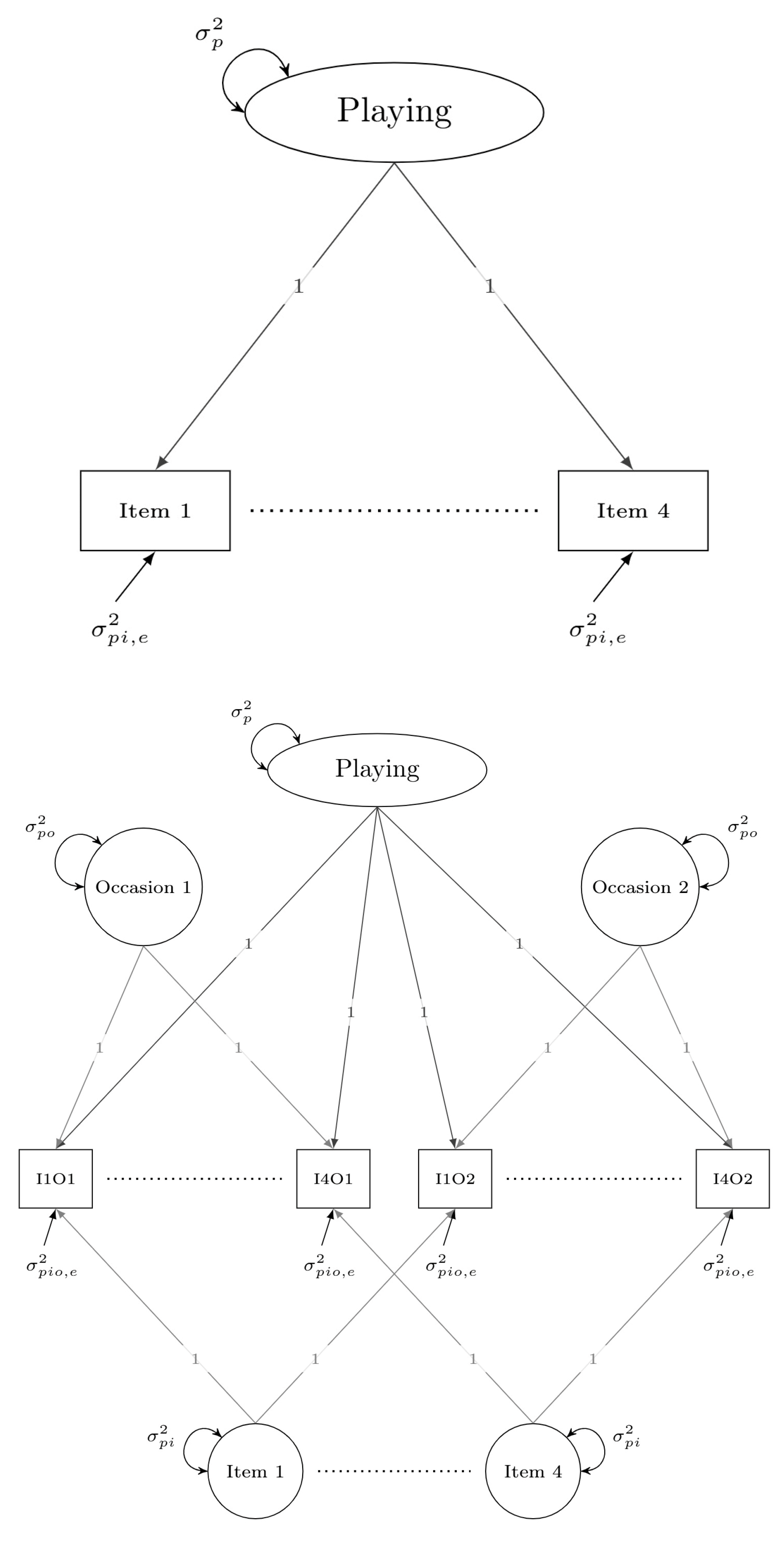
2.2.1. Univariate GT Designs

GT persons × items (pi) single-facet univariate designs. In Figure 1, we depict SEM diagrams for univariate pi and pio designs. The top diagram in Figure 1 represents a pi SEM for the Instrument Playing subscale. The SEM has a single factor for the construct of interest that is linked to all items measuring that construct. Item loadings are set equal to one, and all item uniquenesses are set equal. In total, two parameters are estimated, which represent the variance component for person or universe scores (${\sigma }_p^2$) and the variance component for relative measurement error across items (${\sigma }_{pi,e}^2$).

When using the indicator-mean method [107], the remaining variance component for items (${\sigma }_i^2$) in the pi design is estimated using intercepts for items that are equivalent to their associated means. Specifically, the squared differences between each item mean and grand mean across items are summed and divided by the number of items minus one, as shown in

Table 1. Formulas for variance components within GT univariate pi and pio designs.

Design/VC	Formula
pi design
p	${\widehat{\sigma }}_p^2$
pi,e	${\widehat{\sigma }}_{pi,e}^2$
i	${\widehat{\sigma }}_i^2={\displaystyle \frac{\sum _{i=1}^{n_I}{\left({\widehat{\beta }}_i-grand\widehat{\mu }\right)}^2}{n_I-1}},$ $\mathrm{where} n_I$$=\mathrm{the} \mathrm{total} \mathrm{number} \mathrm{of} \mathrm{items}, {\widehat{\beta }}_i$$=\mathrm{intercept} \mathrm{for} \mathrm{the} i_{th}$$\mathrm{item}, \mathrm{and} grand\widehat{\mu }={\displaystyle \frac{\sum _{i=1}^{n_I}{\widehat{\beta }}_i}{n_I}}$.
pio design
p	${\widehat{\sigma }}_p^2$
pi	${\widehat{\sigma }}_{pi}^2$
po	${\widehat{\sigma }}_{po}^2$
pio,e	${\widehat{\sigma }}_{pio,e}^2$
i	${\widehat{\sigma }}_i^2={\displaystyle \frac{\sum _{i=1}^{n_I}{\left({\widehat{\mu }}_i-grand\widehat{\mu }\right)}^2}{n_I-1}},$ $\mathrm{where} grand\widehat{\mu }={\displaystyle \frac{\sum _{i=1,o=1}^{{i=n_I,o=n}_O}{\widehat{\beta }}_{io}}{n_I\times n_O}},{{\widehat{\beta }}_{io}=\mathrm{i}\mathrm{n}\mathrm{t}\mathrm{e}\mathrm{r}\mathrm{c}\mathrm{e}\mathrm{p}\mathrm{t} \mathrm{f}\mathrm{o}\mathrm{r}\mathrm{t}\mathrm{h}\mathrm{e} i_{th} \mathrm{i}\mathrm{t}\mathrm{e}\mathrm{m} \mathrm{o}\mathrm{n} \mathrm{t}\mathrm{h}\mathrm{e} o_{th} \mathrm{o}\mathrm{c}\mathrm{c}\mathrm{a}\mathrm{s}\mathrm{i}\mathrm{o}\mathrm{n},n}_O=\mathrm{t}\mathrm{h}\mathrm{e} \mathrm{t}\mathrm{o}\mathrm{t}\mathrm{a}\mathrm{l} \mathrm{n}\mathrm{u}\mathrm{m}\mathrm{b}\mathrm{e}\mathrm{r} \mathrm{o}\mathrm{f} \mathrm{o}\mathrm{c}\mathrm{c}\mathrm{a}\mathrm{s}\mathrm{i}\mathrm{o}\mathrm{n}\mathrm{s},\mathrm{a}\mathrm{n}\mathrm{d}$${\widehat{\mu }}_i={\displaystyle \frac{\sum _{o=1}^{n_O}{\widehat{\beta }}_{io}}{n_O}}$.
o	${\widehat{\sigma }}_o^2={\displaystyle \frac{\sum _{o=1}^{n_O}{\left({\widehat{\mu }}_o-grand\widehat{\mu }\right)}^2}{n_O-1}},$$\mathrm{where} {\widehat{\mu }}_o={\displaystyle \frac{\sum _{i=1}^{n_I}{\widehat{\beta }}_{io}}{n_I}}.$
io	${\widehat{\sigma }}_{io}^2={\displaystyle \frac{\sum _{i=1,o=1}^{i=n_I,o=n_O}{\left({\widehat{\beta }}_{io}-{\widehat{\mu }}_i-{\widehat{\mu }}_o+grand\widehat{\mu }\right)}^2}{(n_I\times n_O)-1}}.$

Note. GT = generalizability theory. Variance components without formulas come directly from structural equation model computer output (see Figure 1 and Supplemental Materials).

. Once the three variance components of interest (${\sigma }_p^2,{\sigma }_{pi,e}^2,\mathrm{a}\mathrm{n}\mathrm{d}{\sigma }_i^2$) are estimated. They can be placed in the general equations shown in

Table 2. Formulas for estimating GT G, global D, and cut-score-specific D coefficients for all designs and models.

Design/Index	Formula
pi design
G	${\displaystyle \frac{{\widehat{\sigma }}_p^2}{{\widehat{\sigma }}_p^2+\frac{{\widehat{\sigma }}_{pi,e}^2}{n_i^{\mathrm{’}}}}}$
${\widehat{\omega }}_{H_{Composite}}$	${\displaystyle \frac{{\widehat{\sigma }}_{Gen}^2}{{\widehat{\sigma }}_p^2+\frac{{\widehat{\sigma }}_{pi,e}^2}{n_i^{\mathrm{’}}}}}$
${\widehat{\omega }}_{H_{Subscale}}$	${\displaystyle \frac{{\widehat{\sigma }}_{Grp}^2}{{\widehat{\sigma }}_p^2+\frac{{\widehat{\sigma }}_{pi,e}^2}{n_i^{\mathrm{’}}}}}$
Global D	${\displaystyle \frac{{\widehat{\sigma }}_p^2}{{\widehat{\sigma }}_p^2+\frac{{\widehat{\sigma }}_{pi,e}^2+{\widehat{\sigma }}_i^2}{n_i^{\mathrm{’}}}}}$
Cut-score-specific D	${\displaystyle \frac{{\widehat{\sigma }}_p^2+{\left({\mu }_Y-Cut score\right)}^2-{\widehat{\sigma }}_{\stackrel{-}{Y}}^2}{{\widehat{\sigma }}_p^2+{\left({\mu }_Y-Cut score\right)}^2-{\widehat{\sigma }}_{\stackrel{-}{Y}}^2+\frac{{\widehat{\sigma }}_{pi,e}^2+{\widehat{\sigma }}_i^2}{n_i^{\mathrm{’}}}}}, \mathrm{where} {\widehat{\mathsf{\sigma }}}_{\stackrel{-}{Y}}^2={\displaystyle \frac{{\widehat{\sigma }}_p^2}{n_p^{\mathrm{’}}}}+{\displaystyle \frac{{\widehat{\sigma }}_{pi,e}^2}{n_i^{\mathrm{’}}}}+{\displaystyle \frac{{\widehat{\sigma }}_i^2}{n_i^{\mathrm{’}}}} \mathrm{and} \mathrm{corrects} \mathrm{for} \mathrm{bias}.$
Total relative error	$1-{\displaystyle \frac{{\widehat{\sigma }}_p^2}{{\widehat{\sigma }}_p^2+\frac{{\widehat{\sigma }}_{pi,e}^2}{n_i^{\mathrm{’}}}}}$
pio design
G	${\displaystyle \frac{{\widehat{\sigma }}_p^2}{{\widehat{\sigma }}_p^2+\frac{{\widehat{\sigma }}_{pi}^2}{n_i^{\mathrm{’}}}+\frac{{\widehat{\sigma }}_{po}^2}{n_o^{\mathrm{’}}}+\frac{{\widehat{\sigma }}_{pio,e}^2}{n_i^{\mathrm{’}}{n}_o^{\mathrm{’}}}}}$
${\widehat{\omega }}_{H_{Composite}}$	${\displaystyle \frac{{\widehat{\sigma }}_{Gen}^2}{{\widehat{\sigma }}_p^2+\frac{{\widehat{\sigma }}_{pi}^2}{n_i^{\mathrm{’}}}+\frac{{\widehat{\sigma }}_{po}^2}{n_o^{\mathrm{’}}}+\frac{{\widehat{\sigma }}_{pio,e}^2}{n_i^{\mathrm{’}}{n}_o^{\mathrm{’}}}}}$
${\widehat{\omega }}_{H_{Subscale}}$	${\displaystyle \frac{{\widehat{\sigma }}_{Grp}^2}{{\widehat{\sigma }}_p^2+\frac{{\widehat{\sigma }}_{pi}^2}{n_i^{\mathrm{’}}}+\frac{{\widehat{\sigma }}_{po}^2}{n_o^{\mathrm{’}}}+\frac{{\widehat{\sigma }}_{pio,e}^2}{n_i^{\mathrm{’}}{n}_o^{\mathrm{’}}}}}$
Global D	${\displaystyle \frac{{\widehat{\sigma }}_p^2}{{\widehat{\sigma }}_p^2+\frac{{\widehat{\sigma }}_{pi}^2+{\widehat{\sigma }}_i^2}{n_i^{\mathrm{’}}}+\frac{{\widehat{\sigma }}_{po}^2+{\widehat{\sigma }}_o^2}{n_o^{\mathrm{’}}}+\frac{{\widehat{\sigma }}_{pio,e}^2+{\widehat{\sigma }}_{io}^2}{n_i^{\mathrm{’}}{n}_o^{\mathrm{’}}}}}$
Cut-score-specific D	${\displaystyle \frac{{\widehat{\sigma }}_p^2+{\left({\mu }_Y-Cut score\right)}^2-{\widehat{\sigma }}_{\stackrel{-}{Y}}^2}{{\widehat{\sigma }}_p^2+{\left({\mu }_Y-Cut score\right)}^2-{\widehat{\sigma }}_{\stackrel{-}{Y}}^2+\frac{{\widehat{\sigma }}_{pi}^2+{\widehat{\sigma }}_i^2}{n_i^{\mathrm{’}}}+\frac{{\widehat{\sigma }}_{po}^2+{\widehat{\sigma }}_o^2}{n_o^{\mathrm{’}}}+\frac{{\widehat{\sigma }}_{pio,e}^2+{\widehat{\sigma }}_{io}^2}{n_i^{\mathrm{’}}{n}_o^{\mathrm{’}}}}},$ $\mathrm{where} {\widehat{\mathsf{\sigma }}}_{\stackrel{-}{Y}}^2={\displaystyle \frac{{\widehat{\sigma }}_p^2}{n_p^{\mathrm{’}}}}+{\displaystyle \frac{{\widehat{\sigma }}_{pi}^2}{n_p^{\mathrm{’}}{n}_i^{\mathrm{’}}}}+{\displaystyle \frac{{\widehat{\sigma }}_{po}^2}{n_p^{\mathrm{’}}{n}_o^{\mathrm{’}}}}+{\displaystyle \frac{{\widehat{\sigma }}_{pio,e}^2}{n_p^{\mathrm{’}}{n}_i^{\mathrm{’}}{n}_o^{\mathrm{’}}}}+{\displaystyle \frac{{\widehat{\sigma }}_i^2}{n_i^{\mathrm{’}}}}+{\displaystyle \frac{{\widehat{\sigma }}_o^2}{n_o^{\mathrm{’}}}}+{\displaystyle \frac{{\widehat{\sigma }}_{io}^2}{n_i^{\mathrm{’}}{n}_o^{\mathrm{’}}}} \mathrm{and} \mathrm{corrects} \mathrm{for} \mathrm{bias}.$
Specific-factor error	${\displaystyle \frac{\frac{{\widehat{\sigma }}_{pi}^2}{n_i^{\mathrm{’}}}}{{\widehat{\sigma }}_p^2+\frac{{\widehat{\sigma }}_{pi}^2}{n_i^{\mathrm{’}}}+\frac{{\widehat{\sigma }}_{po}^2}{n_o^{\mathrm{’}}}+\frac{{\widehat{\sigma }}_{pio,e}^2}{n_i^{\mathrm{’}}{n}_o^{\mathrm{’}}}}}$
Transient error	${\displaystyle \frac{\frac{{\widehat{\sigma }}_{po}^2}{n_o^{\mathrm{’}}}}{{\widehat{\sigma }}_p^2+\frac{{\widehat{\sigma }}_{pi}^2}{n_i^{\mathrm{’}}}+\frac{{\widehat{\sigma }}_{po}^2}{n_o^{\mathrm{’}}}+\frac{{\widehat{\sigma }}_{pio,e}^2}{n_i^{\mathrm{’}}{n}_o^{\mathrm{’}}}}}$
Random-response error	${\displaystyle \frac{\frac{{\widehat{\sigma }}_{pio,e}^2}{n_i^{\mathrm{’}}{n}_o^{\mathrm{’}}}}{{\widehat{\sigma }}_p^2+\frac{{\widehat{\sigma }}_{pi}^2}{n_i^{\mathrm{’}}}+\frac{{\widehat{\sigma }}_{po}^2}{n_o^{\mathrm{’}}}+\frac{{\widehat{\sigma }}_{pio,e}^2}{n_i^{\mathrm{’}}{n}_o^{\mathrm{’}}}}}$
Total relative error	$1-{\displaystyle \frac{{\widehat{\sigma }}_p^2}{{\widehat{\sigma }}_p^2+\frac{{\widehat{\sigma }}_{pi}^2}{n_i^{\mathrm{’}}}+\frac{{\widehat{\sigma }}_{po}^2}{n_o^{\mathrm{’}}}+\frac{{\widehat{\sigma }}_{pio,e}^2}{n_i^{\mathrm{’}}{n}_o^{\mathrm{’}}}}}$

Note. pi = persons × items design, pio = persons × items × occasions design, $n_i^{\mathrm{’}}=\mathrm{n}\mathrm{u}\mathrm{m}\mathrm{b}\mathrm{e}\mathrm{r} \mathrm{o}\mathrm{f} \mathrm{i}\mathrm{t}\mathrm{e}\mathrm{m}\mathrm{s} \mathrm{s}\mathrm{p}\mathrm{e}\mathrm{c}\mathrm{i}\mathrm{f}\mathrm{i}\mathrm{e}\mathrm{d},n_o^{\mathrm{’}}=\mathrm{n}\mathrm{u}\mathrm{m}\mathrm{b}\mathrm{e}\mathrm{r} \mathrm{o}\mathrm{f} \mathrm{o}\mathrm{c}\mathrm{c}\mathrm{a}\mathrm{s}\mathrm{i}\mathrm{o}\mathrm{n}\mathrm{s} \mathrm{s}\mathrm{p}\mathrm{e}\mathrm{c}\mathrm{i}\mathrm{f}\mathrm{i}\mathrm{e}\mathrm{d},$ GT = generalizability theory, G = generalizability coefficient, D = dependability coefficient, ${\widehat{\omega }}_{H_{Composite}}$ = Omega hierarchical composite coefficient, ${\widehat{\omega }}_{H_{Subscale}}$ = Omega hierarchical subscale coefficient. Generalizability coefficients for the bifactor model are equivalent to omega total coefficients.

to estimate G, global D, and cut-score-specific D coefficients for the pi design.

GT persons × items × occasions (pio) two-facet univariate designs. The bottom diagram in Figure 1 represents a SEM for the MUSPI-S’s Instrument Playing subscale for a pio design with four items administered on two occasions. When measuring psychological traits, the pio design is generally preferred over the pi design because it allows for the separation of three key sources of measurement error and reduces the confounding of trait and measurement error variance typically found in the pi design. Within the pio SEM shown in Figure 1, the factor for the construct of interest is linked to each item on each occasion. Separate factors are included for each item across all occasions and for each occasion across all items. All factor loadings are set equal to one, with item variances set equal, occasion variances set equal, and uniquenesses set equal. Collectively, these constraints result in the estimation of four parameters to represent the variance of person or universe scores for the construct of interest (${\sigma }_p^2$) and the three primary sources of relative measurement error (${\sigma }_{pi}^2,{\sigma }_{po}^2,\mathrm{a}\mathrm{n}\mathrm{d}{\sigma }_{pio,e}^2$) that affect results when using objectively scored measures such as Likert-style questionnaires or multiple-choice tests in which all scorers would obtain the same results.

Within the psychological research literature, ${\sigma }_{pi}^2,{\sigma }_{po}^2,\mathrm{a}\mathrm{n}\mathrm{d}{\sigma }_{pio,e}^2$ are often, respectively, referred to as specific-factor error (or method effects), transient error (or state effects), and random-response error (or within-occasion “noise” [120,121,122], also see [123]). Specific-factor error represents enduring person-specific effects on scores that are unrelated to the construct of interest such as understandings of words within items and response options. Transient error represents consistent effects on scores within a given occasion that do not generalize across occasions such as respondents’ dispositions, mindsets, and physiological conditions at that time as well as their overall reactions to environmental and administration conditions. Random-response error refers to fleeting moment-to-moment effects within an occasion such as lapses of attention, distractions, and other effects that follow no systematic pattern.

In pi designs, universe score and transient error are confounded within the person variance component (${\sigma }_p^2$), as are specific-factor and random-response error within the relative measurement error component ${(\sigma }_{pi,e}^2).$ This same pattern of confounding mirrors that found in conventional single-occasion reliability coefficients (e.g., alpha, split halves) in relation to true score and measurement error effects. Such confounding can lead to overestimation of score accuracy and underestimation of relationships between underlying constructs when those reliability or corresponding pi design G coefficients are used to disattenuate correlation coefficients between observed scores for measurement error. An important advantage of the pio design is that these sources of variance can be separated to provide more appropriate estimates of score accuracy and overall measurement error. Variance component formulas for each source of measurement error are provided in Table 1.

When using the indicator-mean method to derive the remaining variance components (${\sigma }_i^2, {\sigma }_o^2, \mathrm{a}\mathrm{n}\mathrm{d} {\sigma }_{io}^2$) within the pio design, intercepts will represent means for all combinations of items and occasions. Once estimated, these means can be integrated into the formulas shown in Table 1 to obtain the remaining variance components and insert them into the formulas shown in Table 2 to estimate related indices of score dependability and proportions of measurement error (see [107] for further details).

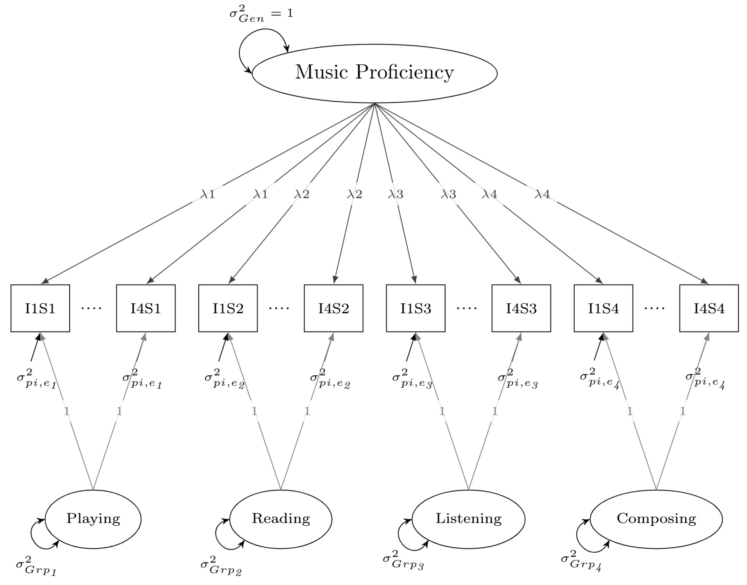
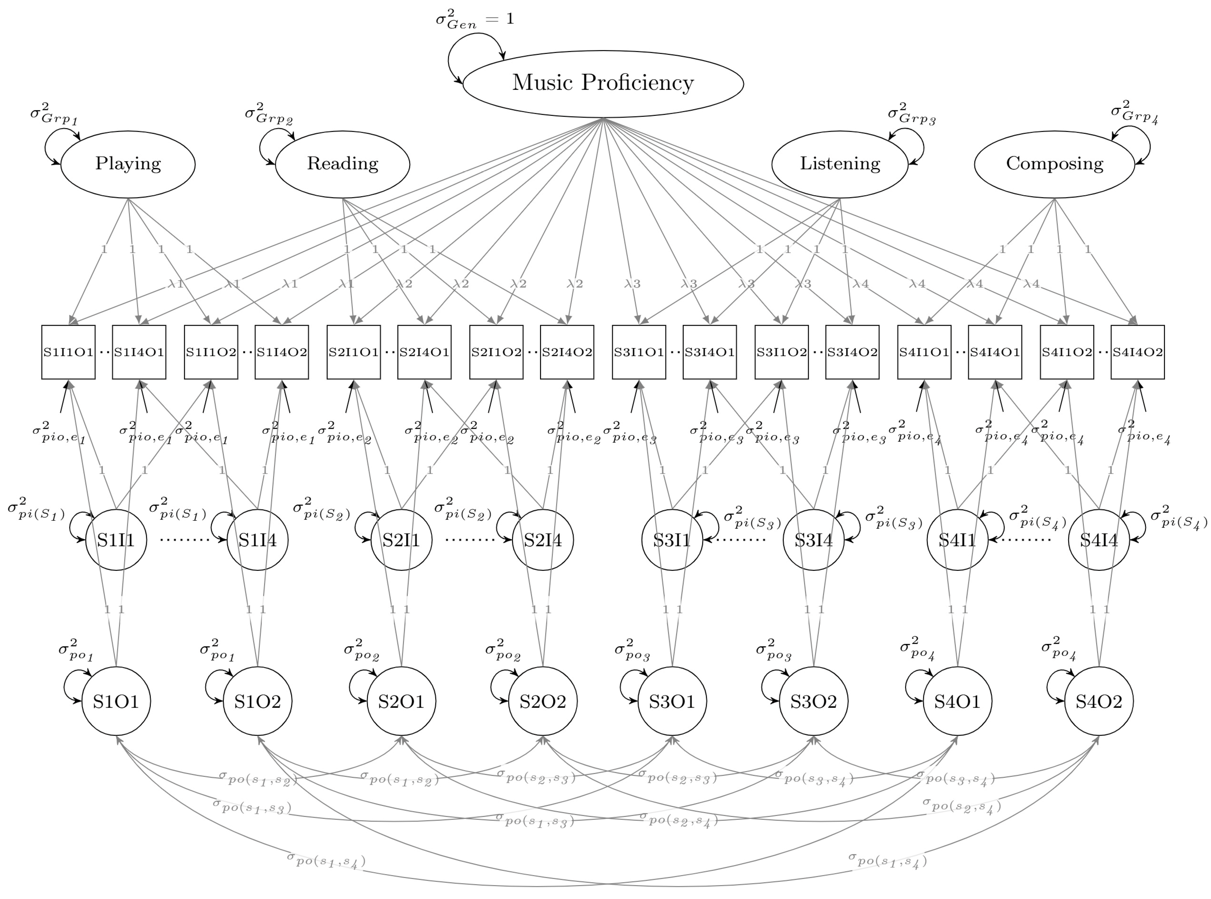
2.2.2. Multivariate GT Designs

GT persons × items (pi) single-facet multivariate designs. Multivariate GT designs best represent indices of score accuracy when both subscale and composite scores are reported in practice. Such designs also can produce correlation coefficients corrected for all sources of measurement error included within a design to provide further insights into subscale score dimensionality, overlap, interrelationships, and validity. Embedded within the overall multivariate design are the same univariate analyses already described for each individual subscale. Variance components for the composite score, in contrast, entail formulas based on the variance components for each subscale, the covariances between each pair of subscale scores, and eventual weighting of each subscale when forming the composite (see

Table 3. Formulas for variance components within GT persons × items (pi) and persons × items × occasions (pio) multivariate designs.

Design/VC	Formula
	Composite	Subscale
pi design
p	${\widehat{\sigma }}_{p_c}^2=\sum _{s=1}^{n_S}{\widehat{\sigma }}_{p_s}^2+\sum _{s1=1}^{n_S}\sum _{s2\ne s1}^{n_S}{\widehat{\sigma }}_{p(s1,s2)}$, $\mathrm{where} n_S$= the total number of subscales.	${\widehat{\sigma }}_{p_s}^2$
pi,e	${\widehat{\sigma }}_{{pi,e}_c}^2={\displaystyle \sum _{s=1}^{n_S}}{\widehat{\sigma }}_{{pi,e}_s}^2$	${\widehat{\sigma }}_{{pi,e}_s}^2$
i	${\widehat{\sigma }}_{i_c}^2={\displaystyle \sum _{s=1}^{n_S}}\left[{\displaystyle \frac{\sum _{i=1}^{n_{Is}}{\left({\widehat{\beta }}_{i\left(s\right)}-grand{\widehat{\mu }}_s\right)}^2}{n_{Is}-1}}\right] ,$ $\mathrm{where} n_{Is}$= the total number of items in subscale s, ${\widehat{\beta }}_{i\left(s\right)}$$=\mathrm{subscale} s\text{’}\mathrm{s} \mathrm{intercept} \mathrm{for} \mathrm{its} i_{th}$$\mathrm{item}, \mathrm{and} grand{\widehat{\mu }}_s={\displaystyle \frac{\sum _{i=1}^{n_{Is}}{\widehat{\beta }}_{i\left(s\right)}}{n_{Is}}}$.	${\widehat{\sigma }}_{i_s}^2={\displaystyle \frac{\sum _{i=1}^{n_{Is}}{\left({\widehat{\beta }}_{i\left(s\right)}-grand{\widehat{\mu }}_s\right)}^2}{n_{Is}-1}}$
pio design
p	${\widehat{\sigma }}_{p_c}^2={\displaystyle \sum _{s=1}^{n_S}}{\widehat{\sigma }}_{p_s}^2+{\displaystyle \sum _{s1=1}^{n_S}}{\displaystyle \sum _{s2\ne s1}^{n_S}}{\widehat{\sigma }}_{p(s1,s2)}$	${\widehat{\sigma }}_{p_s}^2$
pi	${\widehat{\sigma }}_{{pi}_c}^2={\displaystyle \sum _{s=1}^{n_S}}{\widehat{\sigma }}_{{pi}_s}^2$	${\widehat{\sigma }}_{{pi}_s}^2$
po	${\widehat{\sigma }}_{{po}_c}^2={\displaystyle \sum _{s=1}^{n_S}}{\widehat{\sigma }}_{{po}_s}^2+{\displaystyle \sum _{s1=1}^{n_S}}{\displaystyle \sum _{s2\ne s1}^{n_S}}{\widehat{\sigma }}_{po(s1,s2)}$	${\widehat{\sigma }}_{{po}_s}^2$
pio,e	${\widehat{\sigma }}_{{pio,e}_c}^2={\displaystyle \sum _{s=1}^{n_S}}{\widehat{\sigma }}_{{pio,e}_s}^2$	${\widehat{\sigma }}_{{pio,e}_s}^2$
i	${\widehat{\sigma }}_{i_c}^2={\displaystyle \sum _{s=1}^{n_S}}\left[{\displaystyle \frac{\sum _{i=1}^{n_{Is}}{\left({\widehat{\mu }}_{is}-grand{\widehat{\mu }}_s\right)}^2}{n_{Is}-1}}\right] ,$ $\mathrm{where} grand{\widehat{\mu }}_s={\displaystyle \frac{\sum _{i=1,o=1}^{{i=n_{Is},o=n}_{Os}}{\widehat{\beta }}_{io\left(s\right)}}{n_{Is}\times n_{Os}}}, {\widehat{\beta }}_{io\left(s\right)}=\mathrm{s}\mathrm{u}\mathrm{b}\mathrm{s}\mathrm{c}\mathrm{a}\mathrm{l}\mathrm{e}{s}^{\mathrm{’}}\mathrm{s} \mathrm{i}\mathrm{n}\mathrm{t}\mathrm{e}\mathrm{r}\mathrm{c}\mathrm{e}\mathrm{p}\mathrm{t} \mathrm{f}\mathrm{o}\mathrm{r} \mathrm{i}\mathrm{t}\mathrm{s} i_{th} \mathrm{i}\mathrm{t}\mathrm{e}\mathrm{m} \mathrm{a}\mathrm{n}\mathrm{d} i_{th} \mathrm{o}\mathrm{c}\mathrm{c}\mathrm{a}\mathrm{s}\mathrm{i}\mathrm{o}\mathrm{n},$ $and$${\widehat{\mu }}_{is}={\displaystyle \frac{\sum _{o=1}^{n_{Os}}{\widehat{\beta }}_{io\left(s\right)}}{n_{Os}}}$.	${\widehat{\sigma }}_{i_s}^2={\displaystyle \frac{\sum _{i=1}^{n_{Is}}{\left({\widehat{\mu }}_{is}-grand{\widehat{\mu }}_s\right)}^2}{n_{Is}-1}}$
o	${\widehat{\sigma }}_{o_c}^2={\displaystyle \sum _{s=1}^{n_S}}\left[{\displaystyle \frac{\sum _{o=1}^{n_{Os}}{\left({\widehat{\mu }}_{os}-grand{\widehat{\mu }}_s\right)}^2}{n_{Os}-1}}\right]+{\displaystyle \sum _{s1=1}^{n_S}}{\displaystyle \sum _{s2\ne s1}^{n_S}}\left[{\displaystyle \frac{\sum _{o=1}^{n_{Os}}\left({\widehat{\mu }}_{os1}-grand{\widehat{\mu }}_{s1}\right)\left({\widehat{\mu }}_{os2}-grand{\widehat{\mu }}_{s2}\right)}{n_{Os}-1}}\right] ,$ $\mathrm{where} n_{Os}$= the number of occasions for subscales, $\mathrm{and} {\widehat{\mu }}_{os}={\displaystyle \frac{\sum _{i=1}^{n_{Is}}{\widehat{\beta }}_{io\left(s\right)}}{n_{Is}}} .$	${\widehat{\sigma }}_{o_s}^2={\displaystyle \frac{\sum _{o=1}^{n_{Os}}{\left({\widehat{\mu }}_{os}-grand{\widehat{\mu }}_s\right)}^2}{n_{Os}-1}}$
io	${\widehat{\sigma }}_{{io}_c}^2={\displaystyle \sum _{s=1}^{n_S}}\left[{\displaystyle \frac{\sum _{i=1,o=1}^{{i=n}_{Is},o=n_{Os}}{\left({\widehat{\beta }}_{io\left(s\right)}-{\widehat{\mu }}_{is}-{\widehat{\mu }}_{os}+grand{\widehat{\mu }}_s\right)}^2}{(n_{Is}\times n_{Os})-1}}\right]$	${\widehat{\sigma }}_{{io}_s}^2={\displaystyle \frac{\sum _{i=1,o=1}^{{i=n}_{Is},o=n_{Os}}{\left({\widehat{\beta }}_{io\left(s\right)}-{\widehat{\mu }}_{is}-{\widehat{\mu }}_{os}+grand{\widehat{\mu }}_s\right)}^2}{(n_{Is}\times n_{Os})-1}}$

Note. GT = generalizability theory, VC = variance component. Variance components without formulas above come directly from structural equation model computer output (see Figure 2 and Supplemental Materials). Formulas are catered to designs in which persons and occasions are crossed with subscales, and items are nested within subscales.

and [8,64,109]).

Figure 2 includes SEM diagrams for multivariate pi and pio designs that can be used to derive variance and covariance components for computing G coefficients for subscale and composite scores. The diagrams, respectively, represent the 4-item subscales from the MUSPI-S (Instrument Playing, Reading Music, Listening Skill, and Composing Ability) mentioned earlier administered on one or two occasions. Scores for each individual subscale are modeled and constrained in the same way as in a univariate analysis but allowed to covary/correlate with each other. Within the pi design, eight variance components (${\sigma }_p^2 \mathrm{a}\mathrm{n}\mathrm{d} {\sigma }_{pi,e}^2$ for each subscale) and six covariance components (one for each possible pair of subscale scores) are estimated. The variance component for items (${\sigma }_i^2$) within each subscale is computed in the same way as described for the univariate design. The ${\sigma }_p^2,{\sigma }_{pi,e}^2,\mathrm{a}\mathrm{n}\mathrm{d} {\sigma }_i^2 \mathrm{i}\mathrm{n}\mathrm{d}\mathrm{i}\mathrm{c}\mathrm{e}\mathrm{s}$ for the composite score can be estimated using the formulas shown in Table 3, and corresponding generalizability and dependability coefficients using the formulas shown in Table 2.

GT persons × items × occasions (pio) two-facet multivariate designs. The pio univariate design for each embedded subscale within the multivariate design has additional factors for each item across occasions and for each occasion across items. The scores for each pair of subscales are allowed to covary/correlate within an occasion but to the same degree across occasions. Transient error (${\sigma }_{po}^2,$) indices also are allowed to covary/correlate in a similar fashion when all measures are administered together within a common occasion. In all, sixteen variance components ${ (\sigma }_p^2, {\sigma }_{pi}^2,{\sigma }_{po}^2, \mathrm{a}\mathrm{n}\mathrm{d} {\sigma }_{pio,e }^2 \mathrm{f}\mathrm{o}\mathrm{r}\mathrm{e}\mathrm{a}\mathrm{c}\mathrm{h}\mathrm{s}\mathrm{u}\mathrm{b}\mathrm{s}\mathrm{c}\mathrm{a}\mathrm{l}\mathrm{e}),$ six covariance components for person subscale scores (${\sigma }_{p(S_i, S_j)};$ one for each possible pair of subscale scores), and six covariances for transient errors (${\sigma }_{po(S_i, S_j)}$) are estimated. The ${\sigma }_i^2, {\sigma }_o^2,\mathrm{a}\mathrm{n}\mathrm{d} {\sigma }_{io}^2$ variance components for each subscale are derived in the same ways described in the univariate designs, and those for the composite score using the formulas provided in Table 3. Formulas for estimating relevant generalizability and dependability coefficients for both subscale and composite scores are given in Table 2.

Correcting correlation coefficients for measurement error. In addition to providing appropriate indices of accuracy for composite and subscale scores, multivariate designs can yield correlations between all pairs of subscale scores corrected for the sources of measurement error estimated within the design. Corrected correlations can be conceptualized in relation to the formula first proposed by Spearman ([124], also see [125]), shown in Equation (6). Within this formula, the correlation coefficient between observed scores for the pair of measures of interest is divided by the square root of the product of their corresponding reliability coefficients to estimate the correlation between true scores for the targeted measures that is free of measurement error. In applications of GT, G coefficients would be substituted for conventional reliability coefficients, and universe scores for true scores.

$${\widehat{\rho }}_{T_x{T}_y}=\hspace{0.33em}{\displaystyle \frac{r_{xy}}{\sqrt{r_{xx\prime }*r_{yy\prime }}}},$$

(6)

where ${\widehat{\rho }}_{T_x{T}_y}$ = estimated correlation between true scores for measures $X$ and $Y$,

$$\begin{gathered} r_{xy}=\mathrm{observed} \mathrm{correlation} \mathrm{coefficient} \mathrm{between} \mathrm{measures} \mathrm{X} \mathrm{and} \mathrm{Y}, r_{x{x}^{\prime }}=\mathrm{reliability} \mathrm{coefficient} \mathrm{for} \mathrm{measure} \mathrm{X}, \\ \mathrm{and} r_{yy\prime }=\mathrm{reliability} \mathrm{coefficient} \mathrm{for} \mathrm{measure} \mathrm{Y}. \end{gathered}$$

2.2.3. Bifactor GT Designs

Bifactor and multivariate GT designs both can be used to simultaneously partition score variance at subscale and composite levels and distinguish multiple sources of measurement error within pio designs. However, bifactor designs further allow for partitioning of universe score variance into general and group factor effects to produce indices reflecting just general factor effects, just group factor effects, or both effects combined. General factor effects reflect common explained variance shared across all indicators, whereas group factor effects reflect unique explained variance, unrelated to general factor variance, that is shared by all indicators representing a given subscale.

Bifactor models produce four key coefficients: omega total composite, omega total subscale, omega hierarchical composite, and omega hierarchical subscale [11,126,127,128,129,130]. Omega total coefficients for composite and subscale scores represent proportions of variance accounted for by both general and group factor effects. They parallel overall G coefficients for the pi and pio univariate and multivariate GT designs, except that universe score variance (${\sigma }_p^2$) represents the sum of general and group factor variances (${\sigma }_{Gen}^2+{\sigma }_{Grp\left(s\right)}^2$; see Table 2). Omega hierarchical composite score coefficients represent the proportion of variance accounted for by the general factor alone, whereas omega hierarchical subscale coefficients represent the proportion of variance accounted for by the group factor alone. We provide formulas for estimating variance components in

Table 4. Formulas for variance components within GT persons × items (pi) and persons × items × occasions (pio) bifactor designs.

Design/VC	Formula
	Composite	Subscale
pi design
General	${\widehat{\sigma }}_{{Gen}_c}^2=\sum _{s=1}^{n_S}{{\widehat{\lambda }}_s}^2$, where $n_S$ = the total number of subscales.	${\widehat{\sigma }}_{{Gen}_s}^2={{\widehat{\lambda }}_s}^2$
Group	${\widehat{\sigma }}_{{Grp}_c}^2={\displaystyle \sum _{s=1}^{n_S}}{\widehat{\sigma }}_{{Grp}_s}^2$	${\widehat{\sigma }}_{{Grp}_s}^2$
p	${\widehat{\sigma }}_{p_c}^2={\displaystyle \sum _{s=1}^{n_S}}\left[{{\widehat{\lambda }}_s}^2+{\widehat{\sigma }}_{{Grp}_s}^2\right]$	${\widehat{\sigma }}_{p_s}^2={{\widehat{\lambda }}_s}^2+{\widehat{\sigma }}_{{Grp}_s}^2$
pi,e	${\widehat{\sigma }}_{{pi,e}_c}^2={\displaystyle \sum _{s=1}^{n_S}}{\widehat{\sigma }}_{{pi,e}_s}^2$	${\widehat{\sigma }}_{{pi,e}_s}^2$
i	${\widehat{\sigma }}_{i_c}^2={\displaystyle \sum _{s=1}^{n_S}}\left[{\displaystyle \frac{\sum _{i=1}^{n_{Is}}{\left({\widehat{\beta }}_{i\left(s\right)}-grand{\widehat{\mu }}_s\right)}^2}{n_{Is}-1}}\right] ,$ where $n_{Is}$ = the total number of items in subscale s, ${\widehat{\beta }}_{i\left(s\right)}$= subscale s‘s intercept for its $i_{th}$ item, and $grand{\widehat{\mu }}_s={\displaystyle \frac{\sum _{i=1}^{n_{Is}}{\widehat{\beta }}_{i\left(s\right)}}{n_{Is}}}$.	${\widehat{\sigma }}_{i_c}^2={\displaystyle \frac{\sum _{i=1}^{n_{Is}}{\left({\widehat{\beta }}_{i\left(s\right)}-grand{\widehat{\mu }}_s\right)}^2}{n_{Is}-1}}$
pio design
General	${\widehat{\sigma }}_{{Gen}_c}^2={\displaystyle \sum _{s=1}^{n_S}}{{\widehat{\lambda }}_s}^2$	${\widehat{\sigma }}_{{Gen}_s}^2={{\widehat{\lambda }}_s}^2$
Group	${\widehat{\sigma }}_{{Grp}_c}^2={\displaystyle \sum _{s=1}^{n_S}}{\widehat{\sigma }}_{{Grp}_s}^2$	${\widehat{\sigma }}_{{Grp}_s}^2$
p	${\widehat{\sigma }}_{p_c}^2={\displaystyle \sum _{s=1}^{n_S}}\left[{{\widehat{\lambda }}_s}^2+{\widehat{\sigma }}_{{Grp}_s}^2\right]$	${\widehat{\sigma }}_{p_s}^2={{\widehat{\lambda }}_s}^2+{\widehat{\sigma }}_{{Grp}_s}^2$
pi	${\widehat{\sigma }}_{{pi}_c}^2={\displaystyle \sum _{s=1}^{n_S}}{\widehat{\sigma }}_{{pi}_s}^2$	${\widehat{\sigma }}_{{pi}_s}^2$
po	${\widehat{\sigma }}_{{po}_c}^2={\displaystyle \sum _{s=1}^{n_S}}{\widehat{\sigma }}_{{po}_s}^2+{\displaystyle \sum _{s1=1}^{n_S}}{\displaystyle \sum _{s2\ne s1}^{n_S}}{\widehat{\sigma }}_{po(s1,s2)}$	${\widehat{\sigma }}_{{po}_s}^2$
pio,e	${\widehat{\sigma }}_{{pio,e}_c}^2={\displaystyle \sum _{s=1}^{n_S}}{\widehat{\sigma }}_{{pio,e}_s}^2$	${\widehat{\sigma }}_{{pio,e}_s}^2$
i	${\widehat{\sigma }}_{i_c}^2={\displaystyle \sum _{s=1}^{n_S}}\left[{\displaystyle \frac{\sum _{i=1}^{n_{Is}}{\left({\widehat{\mu }}_{is}-grand{\widehat{\mu }}_s\right)}^2}{n_{Is}-1}}\right] ,$ where $grand{\widehat{\mu }}_s={\displaystyle \frac{\sum _{i=1,o=1}^{{i=n_{Is},o=n}_{Os}}{\widehat{\beta }}_{io\left(s\right)}}{n_{Is}\times n_{Os}}}, {\widehat{\beta }}_{io\left(s\right)}=\mathrm{s}\mathrm{u}\mathrm{b}\mathrm{s}\mathrm{c}\mathrm{a}\mathrm{l}\mathrm{e}{s}^{\mathrm{’}}\mathrm{s} \mathrm{i}\mathrm{n}\mathrm{t}\mathrm{e}\mathrm{r}\mathrm{c}\mathrm{e}\mathrm{p}\mathrm{t} \mathrm{f}\mathrm{o}\mathrm{r} \mathrm{i}\mathrm{t}\mathrm{s} i_{th} \mathrm{i}\mathrm{t}\mathrm{e}\mathrm{m} \mathrm{a}\mathrm{n}\mathrm{d} i_{th} \mathrm{o}\mathrm{c}\mathrm{c}\mathrm{a}\mathrm{s}\mathrm{i}\mathrm{o}\mathrm{n},$ $and$ ${\widehat{\mu }}_{is}={\displaystyle \frac{\sum _{o=1}^{n_{Os}}{\widehat{\beta }}_{io\left(s\right)}}{n_{Os}}}$.	${\widehat{\sigma }}_{i_s}^2={\displaystyle \frac{\sum _{i=1}^{n_{Is}}{\left({\widehat{\mu }}_{is}-grand{\widehat{\mu }}_s\right)}^2}{n_{Is}-1}}$
o	${\widehat{\sigma }}_{o_c}^2={\displaystyle \sum _{s=1}^{n_S}}\left[{\displaystyle \frac{\sum _{o=1}^{n_{Os}}{\left({\widehat{\mu }}_{os}-grand{\widehat{\mu }}_s\right)}^2}{n_{Os}-1}}\right]+{\displaystyle \sum _{s1=1}^{n_S}}{\displaystyle \sum _{s2\ne s1}^{n_S}}\left[{\displaystyle \frac{\sum _{o=1}^{n_{Os}}\left({\widehat{\mu }}_{os1}-grand{\widehat{\mu }}_{s1}\right)\left({\widehat{\mu }}_{os2}-grand{\widehat{\mu }}_{s2}\right)}{n_{Os}-1}}\right] ,$ where $n_{Os}$= the total number of occasions for subscales, and ${\widehat{\mu }}_{os}={\displaystyle \frac{\sum _{i=1}^{n_{Is}}{\widehat{\beta }}_{io\left(s\right)}}{n_{Is}}} .$	${\widehat{\sigma }}_{o_s}^2={\displaystyle \frac{\sum _{o=1}^{n_{Os}}{\left({\widehat{\mu }}_{os}-grand{\widehat{\mu }}_s\right)}^2}{n_{Os}-1}}$
io	${\widehat{\sigma }}_{{io}_c}^2={\displaystyle \sum _{s=1}^{n_S}}\left[{\displaystyle \frac{\sum _{i=1,o=1}^{{i=n}_{Is},o=n_{Os}}{\left({\widehat{\beta }}_{io\left(s\right)}-{\widehat{\mu }}_{is}-{\widehat{\mu }}_{os}+grand{\widehat{\mu }}_s\right)}^2}{(n_{Is}\times n_{Os})-1}}\right]$	${\widehat{\sigma }}_{{io}_s}^2={\displaystyle \frac{\sum _{i=1,o=1}^{{i=n}_{Is},o=n_{Os}}{\left({\widehat{\beta }}_{io\left(s\right)}-{\widehat{\mu }}_{is}-{\widehat{\mu }}_{os}+grand{\widehat{\mu }}_s\right)}^2}{(n_{Is}\times n_{Os})-1}}$

Note. GT = generalizability theory, VC = variance component. Variance components without formulas come directly from structural equation model computer output (see Figure 3 and Supplemental Materials). Formulas are catered to designs in which persons and occasions are crossed with subscales, and items are nested within subscales.

that can be inserted into formulas shown in Table 2 to derive G, global D, cut-score-specific D, and omega coefficients for pi and pio bifactor designs.

GT persons × items (pi) single-facet bifactor designs. The pi bifactor SEM representing MUSPI-S scores is shown in the top diagram within Figure 3. The general factor is linked to all items, with independent group factors linked only to items included within each subscale. To allow for differential general factor effects across subscales, model identification constraints differ somewhat from those in the previous designs. Specifically, variances for the general factor and loadings for the group factors are set equal to one, and general factor loadings, group factor variances, and uniquenesses are estimated, but set equal within but not across subscales. In all, twelve parameters are estimated (λ, ${\sigma }_{grp}^2$& ${\sigma }_{pi,e }^2$ for each subscale).

GT persons × items × occasions (pio) two-facet bifactor designs. The bottom diagram in Figure 3 represents the pio bifactor design. It has the same constraints as the pi design, but with additional factors included for occasions and items. Item and occasion factor loadings are set equal to one, with item factor variances, occasion factor variances, and uniquenesses estimated. As in the multivariate pio design, separate occasion factors are included for each subscale that are allowed to covary/correlate with each other but to the same degree across occasions. Five parameters are estimated for each subscale (λ, ${\sigma }_{grp}^2, {\sigma }_{pi }^2, {\sigma }_{po}^2$, ${\& \sigma }_{pio,e }^2$) as well as six additional covariances to model possible correlated within occasion transient error effects.

2.3. Evaluating Subscale Viability Within GT Multivariate and Bifactor Designs

An important question to consider whenever using measures that produce both composite and subscale scores in practice is the extent to which subscale scores yield useful information beyond the composite score. To address this question, Haberman ([131], also see [132,133,134,135]) devised a classical test theory-based procedure to determine whether a subscale’s true scores are better estimated using subscale or composite observed scores. Vispoel and colleagues [64,104,105,110,111] later adapted this procedure to single- and multi-facet GT multivariate and bifactor designs by replacing true score with universe score estimation.

Haberman’s method is based on comparison of indices for subscale and composite scores reflecting proportional reduction in mean-squared error (PRMSE). The PRMSE for the subscale is equivalent to its conventional reliability or GT-based generalizability coefficient, whereas the PRMSE(C) for the composite can be derived using Equation (7).

$$\mathrm{PRMSE}\left(C\right)=r_{T_{S_j},T_C}^2\mathrm{\ast }{r}_{X_C,X_C\mathrm{’}}={\displaystyle \frac{{\widehat{\sigma }}_{T_{S_j},T_C}^2}{{\widehat{\sigma }}_{T_{S_j}}^2\mathrm{\ast }{\widehat{\sigma }}_{T_C}^2}}\mathrm{\ast }{\displaystyle \frac{{\widehat{\sigma }}_{T_C}^2}{{\widehat{\sigma }}_{X_C}^2}}={\displaystyle \frac{{\left({\widehat{\sigma }}_{T_{S_j}}^2+{\sum }_{j\ne k}{\widehat{\sigma }}_{T_{S_j},T_{S_k}}\right)}^2}{{\widehat{\sigma }}_{T_{S_j}}^2\mathrm{\ast }{\widehat{\sigma }}_{X_C}^2}},$$

(7)

where $T=\mathrm{true} \mathrm{score}$, $X=\mathrm{observed} \mathrm{score}$, $S=\mathrm{subscale}$, $C=\mathrm{composite} \mathrm{score}$, and $r_{X_C,X_C\mathrm{’}}$ = composite reliability.

Conceptually, a PRMSE index represents an estimate of the proportion of true or universe score variance accounted for by the targeted observed scores (subscale or composite). Once PRMSEs are obtained for a subscale and its associated composite, they can be inserted into Equation (8) to form a value-added ratio (VAR; see [136]). Subscale viability is increasingly supported as VARs deviate upwardly from 1.00.

$$\mathrm{Value}-\mathrm{Added} \mathrm{Ratio} \left(\mathrm{VAR}\right)=\hspace{0.33em}{\displaystyle \frac{PRMSE\left(Subscale\right)}{PRMSE\left(Composite\right)}}.\hspace{0.33em}$$

(8)

2.4. Comparing GT Univariate, Multivariate, and Bifactor Designs

As previously noted, univariate and multivariate GT designs will produce the same results for individual subscales because univariate designs for subscales are embedded within the overall multivariate design. However, two additional benefits of multivariate over univariate designs described earlier are that they can produce correlation coefficients between all pairs of subscale scores corrected for the sources of measurement error estimated within the design and yield more appropriate indices of generalizability and dependability for composite scores by taking subscale representation and interrelationships into account. Common findings for multivariate designs across recent studies include stronger relationships between subscale scores when corrected for measurement error in addition to G and D coefficients for composite scores that generally exceed those derived strictly from univariate designs in which subscale representation and interrelationships are ignored [64,110,111].

Either GT multivariate or bifactor designs can produce appropriate G and D coefficients at both composite and subscale levels as well as VARs for all subscale scores. In recent studies of personality constructs, GT multivariate and bifactor designs have produced highly comparable G coefficients, D coefficients, and subscale VARs [64,103,111] but with subscale and composite scores partitioned into general and group factor effects within the bifactor designs to provide additional insights into score dimensionality and overlap among constructs. In the vast majority of bifactor model studies, proportions of general factors exceed proportions of group factor variance at both composite and subscale levels (see, e.g., [102,103,104,105,111,128]).

2.5. Further Advantages of Using SEMs to Perform GT Analyses

Confidence intervals and scale coarseness. Two additional benefits of conducting GT analyses using SEMs are to derive Monte Carlo-based confidence intervals for G, D, and omega coefficients, and to use estimation procedures that correct for scale coarseness effects commonly encountered when analyzing dichotomous or ordinal-level data. When performing SEM analyses using the lavaan package in R [137,138], Monte Carlo-based confidence intervals [139] can be derived for nearly any parameter of interest through linkages with the semTools package [140]. Dichotomous and ordinal data can be transformed to continuous latent variable metrics using diagonally weighted least squares (WLSMV in R) or other relevant estimation procedures (see, e.g., [59,62,64,99,101,103,106,107,108,109,141]). In general, differences in G and D coefficients between observed score and continuous latent variable metrics diminish as the numbers of scale points increase with the largest differences observed when items have only two response options [62,107,141,142].

Missing values. R offers a wide variety of procedures to handle missing responses. Pre-analysis packages in R that replace missing with imputed values include Amelia II [143,144], Hmisc [145], mi [146], mice [147], mitools [148], missForest [149], and mitml [150]. Within the semTools package, the auxiliary, BootMiss-class, and bsBootMiss routines can be linked to lavaan to handle missing data using auxiliary information, multiple imputation, bootstrapping, and related procedures within SEM analyses (see [140] for further details). Finally, if missing values are assumed to be random in nature, the procedures just described can be avoided altogether by requesting full information maximum likelihood parameter estimation when analyzing SEMs. Although the data we analyzed here had no missing values, we provide examples of code within our Supplemental Materials for using the mice (multiple imputation by chained equations) package in R to impute values for missing responses.

3. Investigation

Our main purpose within the present study is to demonstrate how indicator-mean and related procedures can be integrated into SEMs to allow for complete analyses of GT-based univariate, multivariate, and bifactor designs on both observed score and continuous latent response variable metrics. To evaluate the congruence of observed score results between SEM and ANOVA-based procedures, we compare G coefficients, D coefficients, and variance components obtained from the univariate and multivariate GT SEM designs to those obtained from the conventional package mGENOVA [95], which is often considered the gold standard when analyzing multivariate designs. Further comparisons of results involving the GT SEMs are made for composite and subscale scores across the multivariate and bifactor designs, across observed and continuous latent response variable score metrics, and across numbers of item scale points (2, 4, and 8).

In relation to the previous research studies cited here, we anticipate the following results:

• G coefficients, D coefficients, and variance components obtained from the GT-based univariate and multivariate SEMs will be highly congruent with those obtained from mGENOVA.
• Multivariate and bifactor GT SEMs will yield comparable G and D coefficients for subscale and composite scores.
• G and D coefficients for the pi designs will exceed those for the pio designs due to control of fewer sources of measurement error.
• Across all multivariate designs, correlation coefficients between scale scores will be higher after correcting for measurement error, but the differences between corrected and uncorrected coefficients will be greater in pio than in pi designs.
• General factor effects will exceed group factor effects at both subscale and composite levels within the bifactor designs.
• Similar patterns of VARs for subscales will be found across multivariate and bifactor designs.
• Composite and subscale scores will be affected by specific-factor (method), transient (state), and response-random (within-occasion noise) measurement error within the pio designs, but those effects will be greater overall at the subscale than composite level due to inclusion of fewer item scores.
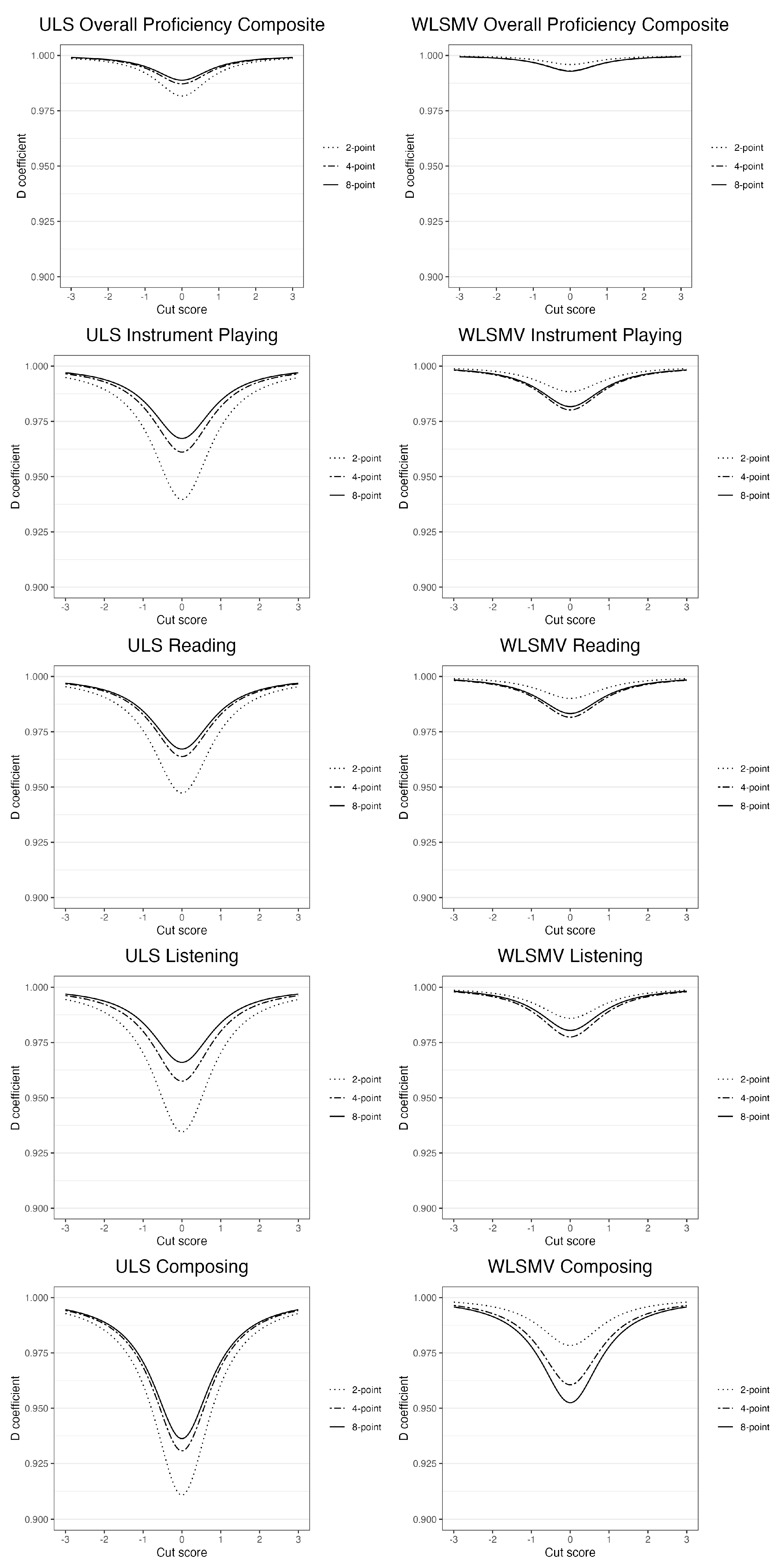
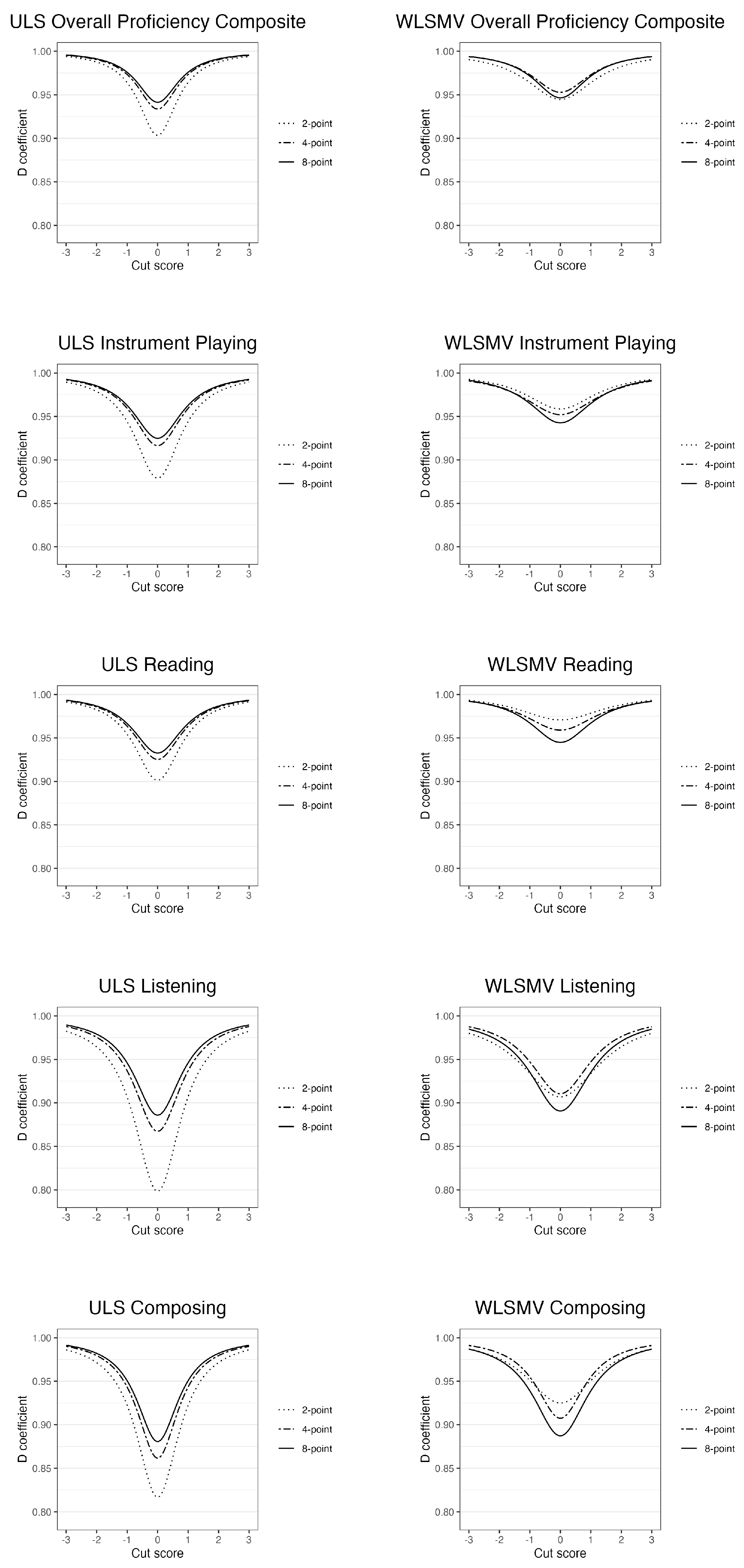
• Differences in G and D coefficients for 2-, 4-, and 8-item scale points will be greater on observed score than on continuous latent response variable metrics.
• G and D coefficients will be greater on continuous latent response variable than on observed score metrics, but to diminishing degrees with increases in numbers of item scale points.

4. Methods

4.1. Participants, Measures, and Procedure

We used the same dataset from Lee and Vispoel [107] in which 511 college students from educational psychology and statistics courses within a large Midwestern university (77.50% female, 82.00 Caucasian, mean age = 21.16) completed the full form of the adult level of the Music Self-Perception Inventory (MUSPI) [116,151,152,153] on two occasions, a week apart. However, for sake of efficiency, variety, and comparison, we analyzed responses to the same subscales (Instrument Playing, Reading Music, Listening, and Composing) using items from the shortened form of the MUSPI (MUSPI-S), all of which are included in the full form.

Each subscale within the MUSPI-S includes four positively phrased items answered along an 8-point item response metric with the following options: (1) Definitely False, (2) Mostly False, (3) Moderately False, (4) More False Than True, (5) More True Than False, (6), Moderately True, (7) Mostly True, (8) Definitely True. We computed subscale scores by adding responses to all items within the given subscale, and composite scores by summing all subscale scores to represent Overall Music Proficiency. Psychometric evidence supporting the use of the MUSPI-S scores includes alpha reliability coefficients for subscale scores no lower than 0.91, confirmatory factor analyses of responses yielding excellent fits to the data, and verification of expected relationships of MUSPI-S subscale scores with each other and with a wide variety of external criterion variables (see, e g., [116,117,118,119]). To evaluate effects of number of item scale points across analyses, we recoded original scores of 1–2, 3–4, 5–6, and 7–8, respectively, to 1, 2, 3, 4 to reduce responses to four scale points, and recoded original scores of 1–4 and 5–8, respectively, to 1 and 2 to reduce responses to two scale points.

4.2. Analyses

Initial analyses included estimation of means, standard deviations, alpha reliability coefficients, and test–retest reliability coefficients for MUSPI-S subscale and composite scores. Subsequent analyses included derivation of variance components, G coefficients, omega coefficients, D coefficients, proportions of measurement error, confidence intervals, correlation coefficients (corrected and uncorrected for measurement error), and VARs for relevant MUSPI-S scales across the pi and pio univariate, multivariate, and bifactor designs. The pi designs include data collected on the first measurement occasion only, and the pio designs include data collected on both occasions. Within the multivariate and bifactor pi and pio designs, items are nested within subscales, and occasions are crossed with subscales in the pio designs. We summarize the overall scope of our primary analyses in Figure 4 in relation to each design.

All SEM-based indices were estimated using procedures within the computer package R. For the sake of comparison, variance components, G coefficients, and D coefficients for observed scores also were derived for univariate and multivariate designs using mGENOVA [96]. To parallel conventional ANOVA-based procedures for observed scores, SEM-based analyses were based on unweighted least squares (ULS) estimation. To convert observed score results to continuous latent response variable metrics in the SEM-based analyses, we used WLSMV estimation within the lavaan package Version 0.6-19 [137,138], which is described by its authors as a diagonally weighted least squares procedure with robust standard errors and a mean and variance adjusted test statistic. We also derived 95% Monte Carlo-based confidence intervals [139] using the semTools package Version 0.5-7 [140] to gauge precision in estimating G, D, and omega coefficients. More detail and computer code for deriving all key indices are provided in our Supplemental Materials.

5. Results

5.1. Means, Standard Deviations, and Conventional Reliability Estimates for MUSPI-S Scores

Table 5. Descriptive statistics and conventional reliability coefficients for MUSPI-S scores.

Metric/Scale	Occasion/Index
	Time 1			Time 2
	Mean Scale (Item)	SD Scale (Item)	$\mathit{\alpha }$	Mean Scale (Item)	SD Scale (Item)	$\mathit{\alpha }$	Test–Retest
2-Point
Composite	22.90 (1.43)	6.06 (0.38)	0.954	23.12 (1.45)	6.15 (0.38)	0.957	0.906
Instrument playing	5.78 (1.44)	1.83 (0.46)	0.940	5.81 (1.45)	1.85 (0.46)	0.946	0.885
Reading music	5.77 (1.44)	1.85 (0.46)	0.948	5.83 (1.46)	1.84 (0.46)	0.942	0.908
Listening	5.78 (1.44)	1.83 (0.46)	0.935	6.12 (1.53)	1.84 (0.46)	0.940	0.799
Composing	5.32 (1.33)	1.67 (0.42)	0.911	5.37 (1.34)	1.73 (0.43)	0.934	0.826
4-Point
Composite	35.83 (2.24)	14.98 (0.94)	0.967	36.48 (2.28)	14.85 (0.93)	0.971	0.936
Instrument playing	9.08 (2.27)	4.46 (1.11)	0.961	9.20 (2.30)	4.41 (1.10)	0.966	0.921
Reading music	9.03 (2.26)	4.52 (1.13)	0.964	9.14 (2.29)	4.38 (1.09)	0.971	0.930
Listening	9.08 (2.27)	4.46 (1.11)	0.958	9.88 (2.47)	4.26 (1.07)	0.959	0.871
Composing	8.06 (2.02)	3.79 (0.95)	0.932	8.26 (2.06)	3.80 (0.95)	0.950	0.870
8-Point
Composite	63.06 (3.94)	31.64 (1.98)	0.971	64.54 (4.03)	31.32 (1.96)	0.975	0.944
Instrument playing	15.97 (3.99)	9.42 (2.36)	0.967	16.29 (4.07)	9.24 (2.31)	0.973	0.929
Reading music	15.91 (3.98)	9.49 (2.37)	0.968	16.12 (4.03)	9.17 (2.29)	0.978	0.937
Listening	15.97 (3.99)	9.42 (2.36)	0.966	17.72 (4.43)	8.79 (2.20)	0.967	0.890
Composing	14.01 (3.50)	7.89 (1.97)	0.937	14.41 (3.60)	7.91 (1.98)	0.958	0.891

Note. MUSPI-S = shortened form of the Music Self-Perception Inventory.

includes means, standard deviations, and alpha reliability estimates for all MUSPI-S scales and response metrics within each occasion, as well as test–retest reliability estimates across occasions. In relation to individual item scale metrics, means for all scales fall near or below their respective scale midpoint values of 1.5, 2.5, and 4.5 for the 2-, 4-, and 8-point metrics, with the Composing subscale always having the lowest mean. Standard deviations for each scale reflect high variability, with ranges of 0.38–0.46, 0.93–1.13, and 1.96–2.37, corresponding to score metrics of 1–2, 1–4, and 1–8. These results make sense given the likely heterogeneity of music-related skills within this college student sample. Across scales and response metrics, alpha coefficients within occasions are uniformly high, ranging from 0.911 to 0.978. Test–retest coefficients range from 0.799 to 0.944 and are lower than corresponding alpha coefficients in all instances, thereby reflecting lower occasion-to-occasion than item-to-item consistency for all MUSPI-S scales represented here.

5.2. GT pi Analyses

5.2.1. Univariate and Multivariate Designs

Analyses using SEMs versus mGENOVA. Results for G coefficients, global D coefficients, and variance components for observed composite scores within the SEM-ULS multivariate designs and their embedded univariate designs for subscales shown in

Table 6. MUSPI-S G coefficients, global D coefficients, and variance components for persons × items multivariate designs.

	Metric/Procedure
	2-Point			4-Point			8-Point
Scale/ Index	mGENOVA	ULS	WLSMV	mGENOVA	ULS	WLSMV	mGENOVA	ULS	WLSMV
Composite
G	0.977	0.977 (0.964, 0.989)	0.996 (0.995, 0.997)	0.985	0.985 (0.983, 0.987)	0.993 (0.992, 0.994)	0.988	0.988 (0.987, 0.988)	0.993 (0.992, 0.994)
Total RE	0.023	0.023	0.004	0.015	0.015	0.007	0.012	0.012	0.007
Global D	0.977	0.977 (0.964, 0.988)	0.996 (0.995, 0.997)	0.985	0.985 (0.983, 0.987)	0.993 (0.992, 0.994)	0.987	0.987 (0.987, 0.988)	0.993 (0.991, 0.994)
${\widehat{\sigma }}_p^2$	0.140	0.140	1.262	0.864	0.864	1.093	3.861	3.861	1.233
${\widehat{\sigma }}_{pi,e}^2$	0.013	0.013	0.020	0.052	0.052	0.031	0.194	0.194	0.036
${\widehat{\sigma }}_i^2$	0.000	0.000	0.000	0.000	0.000	0.000	0.002	0.003	0.001
Instrument playing
G	0.940	0.940 (0.866, 1.000)	0.989 (0.984, 0.993)	0.961	0.961 (0.950, 0.973)	0.980 (0.976, 0.984)	0.967	0.967 (0.965, 0.970)	0.982 (0.979, 0.985)
Total RE	0.060	0.060	0.011	0.039	0.039	0.020	0.033	0.033	0.018
Global D	0.940	0.940 (0.863, 1.000)	0.988 (0.984, 0.993)	0.961	0.961 (0.949, 0.972)	0.980 (0.976, 0.984)	0.967	0.967 (0.965, 0.970)	0.982 (0.978, 0.985)
${\widehat{\sigma }}_p^2$	0.197	0.197	1.995	1.195	1.195	1.869	5.367	5.367	1.771
${\widehat{\sigma }}_{pi,e}^2$	0.050	0.050	0.092	0.192	0.192	0.150	0.722	0.722	0.131
${\widehat{\sigma }}_i^2$	0.000	0.000	0.001	0.000	0.001	0.001	0.002	0.004	0.001
Reading music
G	0.948	0.948 (0.876, 1.000)	0.991 (0.987, 0.994)	0.964	0.964 (0.953, 0.976)	0.982 (0.979, 0.986)	0.968	0.968 (0.966, 0.971)	0.984 (0.982, 0.987)
Total RE	0.052	0.052	0.009	0.036	0.036	0.018	0.032	0.032	0.016
Global D	0.948	0.947 (0.873, 1.000)	0.990 (0.986, 0.994)	0.964	0.964 (0.952, 0.975)	0.982 (0.978, 0.985)	0.967	0.967 (0.965, 0.970)	0.983 (0.980, 0.986)
${\widehat{\sigma }}_p^2$	0.202	0.202	1.556	1.230	1.230	1.364	5.445	5.445	1.768
${\widehat{\sigma }}_{pi,e}^2$	0.045	0.045	0.059	0.181	0.181	0.098	0.715	0.715	0.112
${\widehat{\sigma }}_i^2$	0.000	0.000	0.003	0.003	0.003	0.004	0.021	0.022	0.008
Listening
G	0.935	0.935 (0.860, 1.000)	0.986 (0.981, 0.991)	0.958	0.958 (0.946, 0.969)	0.978 (0.973, 0.982)	0.966	0.966 (0.963, 0.969)	0.981 (0.977, 0.983)
Total RE	0.065	0.065	0.014	0.042	0.042	0.022	0.034	0.034	0.019
Global D	0.935	0.935 (0.857, 0.998)	0.986 (0.981, 0.991)	0.958	0.958 (0.945, 0.969)	0.978 (0.973, 0.982)	0.966	0.966 (0.963, 0.969)	0.980 (0.977, 0.983)
${\widehat{\sigma }}_p^2$	0.196	0.196	1.546	1.158	1.158	1.626	4.927	4.927	1.413
${\widehat{\sigma }}_{pi,e}^2$	0.055	0.055	0.088	0.205	0.205	0.149	0.692	0.692	0.112
${\widehat{\sigma }}_i^2$	0.000	0.000	0.000	0.000	0.000	0.000	0.000	0.000	0.000
Composing
G	0.911	0.911 (0.818, 0.993)	0.979 (0.972, 0.986)	0.932	0.932 (0.915, 0.948)	0.962 (0.954, 0.968)	0.937	0.937 (0.934, 0.941)	0.954 (0.946, 0.960)
Total RE	0.089	0.089	0.021	0.068	0.068	0.038	0.063	0.063	0.046
Global D	0.911	0.911 (0.815, 0.990)	0.978 (0.971, 0.986)	0.931	0.931 (0.914, 0.947)	0.961 (0.953, 0.967)	0.937	0.936 (0.932, 0.940)	0.953 (0.944, 0.959)
${\widehat{\sigma }}_p^2$	0.159	0.159	1.026	0.837	0.837	0.595	3.649	3.649	1.123
${\widehat{\sigma }}_{pi,e}^2$	0.062	0.062	0.088	0.246	0.246	0.095	0.974	0.974	0.218
${\widehat{\sigma }}_i^2$	0.000	0.000	0.003	0.003	0.003	0.002	0.016	0.018	0.006

Note. MUSPI-S = shortened form of the Music Self-Perception Inventory, G = generalizability coefficient, Global D = global dependability coefficient, Total RE = total relative error, ULS = unweighted least squares estimation, WLSMV = diagonally weighted least squares estimation with robust standard errors and a mean and variance adjusted test statistic. Values within parentheses represent 95% confidence interval limits.

are highly consistent with those obtained from the mGENOVA package. Between the two approaches, G coefficients are identical, global D coefficients differ by no more than 0.001, and variance components differ by no more than 0.002.

Score generalizability and global dependability within the SEMs. Across scales and numbers of item scale points, G and global D coefficients for the SEMs are uniformly higher for WLSMV than for ULS estimation, but these differences are noticeably greater for subscale than for composite scores. This indicates that scale coarseness effects can be especially pronounced when using a small number of items. These differences are further exacerbated, but to a lesser degree here, when using more limited numbers of scale points.

Confidence intervals. In relation to widths of confidence intervals (i.e., differences between upper and lower limits) shown in Table 6, precision in estimating G and global D coefficients is weakest with two item scale points and improves with increases in numbers of item scale points for ULS but not always for WLSMV estimates. With 8-point items, widths of confidence intervals are uniformly narrower for ULS than for WLSMV estimation, thereby indicating greater relative increases in precision with increases in item scale points on the observed score metric than on the continuous latent response variable metric.

Cut-score-specific D coefficients. For purposes of comparison, cut-score-specific D coefficients for composite and subscale scores using both ULS and WLSMV estimation are depicted on Z-score metrics (M = 0, SD = 1) in Figure 5. Across scales and estimation procedures, dependability is lowest at the scale mean and progressively increases as scores deviate farther and farther away from the mean. Consistent with the results for G and global D coefficients, composite cut-score-specific D coefficients based on ULS estimates always exceed those for subscales at common standard deviation distances away from the scale mean. As expected, differences in G coefficients, global D coefficients (Table 6), and cut-score-specific D coefficients (Figure 5) for observed scores based on ULS estimation are typically greater between two and four scale points than between four and eight scale points. However, this pattern does not hold for the continuous latent variable response metric based on WLSMV estimation in which corrections for coarseness are greater for 2-point than for 4- or 8-point scales. As scores become increasingly extreme for all scales and estimation procedures, cut-score-specific coefficients across numbers of item scale points begin to coincide, thereby illustrating that the number of scale point effects on score dependability are noticeably greater within the middle of score distributions than at the extremes.

Subscale intercorrelations. As noted earlier, an important advantage of GT multivariate analyses is to produce correlation coefficients between subscale scores corrected for measurement error. As expected, the corrected and uncorrected correlation coefficients between subscales in

Table 7. MUSPI-S subscale correlation coefficients for GT persons × items multivariate designs.

Metric/ Estimator/Subscale	Correlation Coefficient
2-Point/ULS	Instrument playing	Reading music	Listening	Composing
Instrument playing		0.844	0.609	0.626
Reading music	0.797		0.657	0.558
Listening	0.571	0.618		0.646
Composing	0.579	0.518	0.596
2-Point/WLSMV	Instrument playing	Reading music	Listening	Composing
Instrument playing		0.920	0.731	0.749
Reading music	0.910		0.778	0.685
Listening	0.721	0.769		0.784
Composing	0.737	0.675	0.770
4-Point/ULS	Instrument playing	Reading music	Listening	Composing
Instrument playing		0.878	0.678	0.681
Reading music	0.845		0.716	0.617
Listening	0.650	0.689		0.689
Composing	0.645	0.585	0.651
4-Point/WLSMV	Instrument playing	Reading music	Listening	Composing
Instrument playing		0.915	0.736	0.736
Reading music	0.898		0.776	0.679
Listening	0.721	0.760		0.745
Composing	0.715	0.660	0.722
8-Point/ULS	Instrument playing	Reading music	Listening	Composing
Instrument playing		0.884	0.696	0.704
Reading	0.855		0.727	0.652
Listening	0.673	0.703		0.719
Composing	0.671	0.621	0.684
8-Point/WLSMV	Instrument playing	Reading music	Listening	Composing
Instrument playing		0.885	0.725	0.732
Reading music	0.871		0.744	0.685
Listening	0.711	0.731		0.748
Composing	0.708	0.664	0.724

Note. Observed score correlation coefficients are in the lower triangle of the matrices, and corrected (i.e., disattenuated) correlations are in the upper triangle. MUSPI-S = shortened form of the Music Self-Perception Inventory, GT = generalizability theory, ULS = unweighted least squares estimation, WLSMV = diagonally weighted least squares estimation with robust standard errors and a mean and variance adjusted test statistic.

reveal that the relationship between each pair of measured constructs is greater than would otherwise be inferred (ULS: uncorrected $\overline{r}$ = 0.664, corrected $\overline{r}$ = 0.699; WLSMV: uncorrected $\overline{r}$ = 0.748, corrected $\overline{r}$ = 0.764). The modest average differences between corrected and uncorrected coefficients observed here result from the generally high G coefficients for the subscales using either estimation method. Such differences are expected to increase when G coefficients are corrected for additional sources of measurement error (see Equation (6) and results of the pio designs presented in subsequent sections).

5.2.2. Bifactor Designs

Score generalizability and dependability. GT bifactor analyses provide an additional perspective on results by generally yielding G and D coefficients comparable to those obtained from parallel multivariate analyses but further subdividing universe score variance into general and group factor effects. Comparing the G and global D coefficients for the bifactor designs in Table 7 to those for the multivariate designs in Table 6 verifies that this congruence holds, with coefficients being identical with ULS estimation and varying by no more than 0.001 with WLSMV estimation. Accordingly, differences in results between ULS and WLSMV estimation and across numbers of scale points previously discussed for multivariate designs hold here, as do the differences between cut-score-specific D coefficients shown in Figure 5.

General and group factor effects. Relative general and group factor effects on composite and subscale score variance can be examined using omega hierarchical composite (${\widehat{\omega }}_{H_{Composite}}$) and omega hierarchical subscale (${\widehat{\omega }}_{H_{Subscale}}$) coefficients that, respectively, represent proportions of explained general and group factor effects (see

Table 8. MUSPI-S G coefficients, global D coefficients, and variance components for GT persons × items bifactor designs.

	Metric/Procedure
	2-Point		4-Point		8-Point
Scale/Index	ULS	WLSMV	ULS	WLSMV	ULS	WLSMV
Composite
G	0.977 (0.964, 0.989)	0.996 (0.995, 0.997)	0.985 (0.983, 0.987)	0.993 (0.991, 0.994)	0.988 (0.987, 0.988)	0.992 (0.991, 0.993)
${\widehat{\omega }}_{H_{Composite}}$	0.869 (0.837, 0.899)	0.938 (0.925, 0.950)	0.900 (0.895, 0.905)	0.930 (0.918, 0.940)	0.909 (0.908, 0.910)	0.924 (0.913, 0.934)
${\widehat{\omega }}_{H_{Subscale}}$	0.108 (0.073, 0.143)	0.058 (0.046, 0.071)	0.085 (0.080, 0.091)	0.063 (0.053, 0.073)	0.078 (0.077, 0.079)	0.068 (0.060, 0.079)
Total RE	0.023	0.004	0.015	0.007	0.012	0.008
Global D	0.977 (0.963, 0.988)	0.996 (0.995, 0.997)	0.985 (0.983, 0.987)	0.992 (0.991, 0.993)	0.987 (0.987, 0.988)	0.992 (0.991, 0.993)
${\widehat{\sigma }}_p^2$	0.140	4.299	0.863	2.573	3.859	1.982
${\widehat{\sigma }}_{General}^2$	0.125	4.050	0.789	2.411	3.553	1.846
${\widehat{\sigma }}_{Group}^2$	0.015	0.249	0.075	0.162	0.305	0.137
${\widehat{\sigma }}_{pi,e}^2$	0.013	0.071	0.052	0.078	0.194	0.060
${\widehat{\sigma }}_i^2$	0.000	0.002	0.000	0.001	0.003	0.002
Instrument playing
G	0.940 (0.865, 1.000)	0.989 (0.984, 0.993)	0.961 (0.950, 0.973)	0.980 (0.976, 0.984)	0.967 (0.965, 0.970)	0.982 (0.979, 0.985)
${\widehat{\omega }}_{H_{Composite}}$	0.744 (0.568, 0.953)	0.888 (0.830, 0.948)	0.806 (0.774, 0.840)	0.882 (0.843, 0.920)	0.819 (0.811, 0.826)	0.860 (0.826, 0.890)
${\widehat{\omega }}_{H_{Subscale}}$	0.196 (0.000, 0.394)	0.101 (0.042, 0.158)	0.155 (0.118, 0.191)	0.098 (0.062, 0.135)	0.149 (0.140, 0.157)	0.122 (0.094, 0.153)
Total RE	0.060	0.011	0.039	0.020	0.033	0.018
Global D	0.940 (0.863, 1.000)	0.988 (0.984, 0.993)	0.961 (0.949, 0.972)	0.980 (0.976, 0.984)	0.967 (0.965, 0.970)	0.982 (0.978, 0.984)
${\widehat{\sigma }}_p^2$	0.197	5.114	1.195	4.327	5.367	2.621
${\widehat{\sigma }}_{General}^2$	0.156	4.593	1.002	3.895	4.541	2.294
${\widehat{\sigma }}_{Group}^2$	0.041	0.521	0.193	0.432	0.825	0.326
${\widehat{\sigma }}_{pi,e}^2$	0.050	0.237	0.192	0.348	0.722	0.194
${\widehat{\sigma }}_i^2$	0.000	0.004	0.001	0.002	0.004	0.002
Reading music
G	0.948 (0.876, 1.000)	0.991 (0.987, 0.994)	0.964 (0.953, 0.976)	0.982 (0.979, 0.986)	0.968 (0.966, 0.971)	0.984 (0.982, 0.987)
${\widehat{\omega }}_{H_{Composite}}$	0.741 (0.568, 0.941)	0.889 (0.830, 0.947)	0.800 (0.768, 0.833)	0.881 (0.842, 0.920)	0.810 (0.803, 0.818)	0.844 (0.809, 0.876)
${\widehat{\omega }}_{H_{Subscale}}$	0.206 (0.000, 0.401)	0.102 (0.044, 0.159)	0.165 (0.128, 0.200)	0.101 (0.064, 0.139)	0.158 (0.150, 0.166)	0.140 (0.110, 0.174)
Total RE	0.052	0.009	0.036	0.018	0.032	0.016
Global D	0.947 (0.873, 1.000)	0.990 (0.986, 0.994)	0.964 (0.952, 0.975)	0.982 (0.978, 0.985)	0.967 (0.965, 0.970)	0.983 (0.980, 0.986)
${\widehat{\sigma }}_p^2$	0.202	6.891	1.230	2.628	5.445	2.529
${\widehat{\sigma }}_{General}^2$	0.158	6.182	1.020	2.358	4.557	2.169
${\widehat{\sigma }}_{Group}^2$	0.044	0.710	0.210	0.270	0.888	0.360
${\widehat{\sigma }}_{pi,e}^2$	0.045	0.263	0.181	0.189	0.715	0.161
${\widehat{\sigma }}_i^2$	0.000	0.013	0.003	0.008	0.022	0.011
Listening
G	0.935 (0.861, 1.000)	0.986 (0.981, 0.991)	0.958 (0.945, 0.969)	0.978 (0.973, 0.982)	0.966 (0.963, 0.969)	0.981 (0.977, 0.983)
${\widehat{\omega }}_{H_{Composite}}$	0.529 (0.399, 0.684)	0.695 (0.613, 0.776)	0.602 (0.576, 0.628)	0.674 (0.614, 0.730)	0.626 (0.619, 0.632)	0.663 (0.612, 0.709)
${\widehat{\omega }}_{H_{Subscale}}$	0.405 (0.217, 0.559)	0.291 (0.212, 0.373)	0.356 (0.325, 0.386)	0.304 (0.249, 0.362)	0.341 (0.333, 0.348)	0.318 (0.272, 0.367)
Total RE	0.065	0.014	0.042	0.022	0.034	0.019
Global D	0.935 (0.859, 0.999)	0.986 (0.981, 0.991)	0.958 (0.945, 0.969)	0.978 (0.973, 0.981)	0.966 (0.963, 0.969)	0.980 (0.977, 0.983)
${\widehat{\sigma }}_p^2$	0.196	3.577	1.158	2.671	4.927	2.305
${\widehat{\sigma }}_{General}^2$	0.111	2.522	0.727	1.842	3.190	1.558
${\widehat{\sigma }}_{Group}^2$	0.085	1.055	0.430	0.830	1.737	0.747
${\widehat{\sigma }}_{pi,e}^2$	0.055	0.204	0.205	0.245	0.692	0.183
${\widehat{\sigma }}_i^2$	0.000	0.000	0.000	0.000	0.000	0.000
Composing
G	0.911 (0.819, 0.992)	0.979 (0.971, 0.986)	0.932 (0.915, 0.948)	0.962 (0.954, 0.968)	0.937 (0.934, 0.941)	0.954 (0.946, 0.960)
${\widehat{\omega }}_{H_{Composite}}$	0.468 (0.342, 0.626)	0.651 (0.562, 0.735)	0.527 (0.501, 0.556)	0.606 (0.541, 0.667)	0.569 (0.563, 0.576)	0.626 (0.574, 0.675)
${\widehat{\omega }}_{H_{Subscale}}$	0.443 (0.237, 0.606)	0.328 (0.245, 0.415)	0.404 (0.368, 0.438)	0.356 (0.297, 0.417)	0.368 (0.360, 0.377)	0.327 (0.282, 0.375)
Total RE	0.089	0.021	0.068	0.038	0.063	0.046
Global D	0.911 (0.816, 0.989)	0.978 (0.970, 0.985)	0.931 (0.914, 0.947)	0.961 (0.953, 0.967)	0.936 (0.932, 0.940)	0.953 (0.944, 0.959)
${\widehat{\sigma }}_p^2$	0.159	5.052	0.837	2.869	3.649	2.187
${\widehat{\sigma }}_{General}^2$	0.082	3.358	0.474	1.808	2.216	1.436
${\widehat{\sigma }}_{Group}^2$	0.077	1.694	0.363	1.062	1.433	0.751
${\widehat{\sigma }}_{pi,e}^2$	0.062	0.434	0.246	0.459	0.974	0.424
${\widehat{\sigma }}_i^2$	0.000	0.013	0.003	0.011	0.018	0.011

Note. MUSPI-S = shortened form of the Music Self-Perception Inventory, GT = generalizability theory, G = generalizability coefficient, Global D = global dependability coefficient, ${\widehat{\omega }}_{H_{Composite}}$ = Omega hierarchical composite coefficient, ${\widehat{\omega }}_{H_{Subscale}}$ = Omega hierarchical subscale coefficient, Total RE = total relative error, ULS = unweighted least squares estimation, WLSMV = diagonally weighted least squares estimation with robust standard errors and a mean and variance adjusted test statistic. Generalizability coefficients for bifactor model are equivalent to omega total coefficients. Values within parentheses represent 95% confidence interval limits.

). Across numbers of scale points, these coefficients reveal that the strongest general and weakest group factor effects are found for the Overall Music Proficiency composite (${\widehat{\omega }}_{H_{Composite}}$: 0.869–0.938; ${\widehat{\omega }}_{H_{Subscale}}$: 0.058–0.108), Instrument Playing subscale (${\widehat{\omega }}_{H_{Composite}}$: 0.744–0.888; ${\widehat{\omega }}_{H_{Subscale}}$: 0.098–0.196), and Reading Music subscale (${\widehat{\omega }}_{H_{Composite}}$: 0.741–0.889; ${\widehat{\omega }}_{H_{Subscale}}$: 0.101–0.206), whereas the weakest general and strongest group effects are found for the Composing (${\widehat{\omega }}_{H_{Composite}}$: 0.468–0.651; ${\widehat{\omega }}_{H_{Subscale}}$: 0.327–0.443) and Listening (${\widehat{\omega }}_{H_{Composite}}$: 0.529–0.695; ${\widehat{\omega }}_{H_{Subscale}}$: 0.291–0.405) subscales.

Confidence intervals. Precision in estimating G, global D, and omega coefficients in relation to the widths of confidence intervals within the bifactor designs display patterns of G and global D coefficients parallel to those within the corresponding multivariate designs. Widths are generally narrower for composite than for subscale scores, they progressively narrow with increasing numbers of item scale points with ULS estimates, and they narrow when moving from two to either four or eight item scale points with WLSMV estimation, but not necessarily when moving between four to eight item scale points. This same relative pattern of width differences holds for omega hierarchical coefficients.

5.2.3. Subscale Viability

Subscale VARs within GT multivariate and bifactor designs. To use both subscale and composite scores in practice, subscale scores should provide unique information beyond that represented within the composite that subsumes the subscale scores. The VARs for MUSPI-S subscale scores in

Table 9. MUSPI-S subscale value-added ratios for GT persons × items multivariate and bifactor designs.

Design/Subscale	Metric/Estimator
	2-Point		4-Point		8-Point
	ULS	WLSMV	ULS	WLSMV	ULS	WLSMV
Multivariate design
Instrument playing	1.196	1.122	1.154	1.111	1.145	1.136
Reading	1.216	1.134	1.168	1.120	1.155	1.154
Listening	1.338	1.225	1.278	1.217	1.268	1.259
Composing	1.421	1.305	1.373	1.367	1.322	1.289
Bifactor design
Instrument playing	1.185	1.105	1.146	1.093	1.137	1.123
Reading	1.199	1.098	1.153	1.113	1.143	1.137
Listening	1.363	1.272	1.299	1.264	1.287	1.274
Composing	1.438	1.263	1.386	1.292	1.335	1.263

Note. MUSPI-S = shortened form of the Music Self-Perception Inventory, ULS = unweighted least squares estimation, WLSMV = diagonally weighted least squares estimation with robust standard errors and a mean and variance adjusted test statistic.

provide a useful mechanism to verify such expectations within both GT multivariate and bifactor designs. Despite the relatively high correlations between many pairs of subscale scores shown in Table 7, the VARs for all MUSPI-S subscales examined here exceed 1.00, thereby supporting their added value beyond the composite. Consistent with results for omega hierarchical coefficients, VARs are higher for the Composing and Listening subscales than for the Instrument Playing and Reading Music subscales.

5.3. GT pio Analyses

5.3.1. Univariate and Multivariate Designs

Analyses using SEMs versus mGENOVA. As previously noted, pio designs generally provide more appropriate indices of score accuracy for trait-based measures because they allow for the estimation of multiple sources of measurement error (specific-factor, transient, and random-response) that are likely to affect scores. In

Table 10. MUSPI-S G coefficients, global D coefficients, and variance components for GT persons × items × occasions multivariate designs.

Scale/ Index	Metric/Procedure
	2-Point			4-Point			8-Point
	mGENOVA	ULS	WLSMV	mGENOVA	ULS	WLSMV	mGENOVA	ULS	WLSMV
Composite
G	0.904	0.904 (0.853, 0.956)	0.946 (0.925, 0.967)	0.935	0.935 (0.926, 0.943)	0.954 (0.944, 0.964)	0.943	0.943 (0.941, 0.945)	0.948 (0.939, 0.955)
SFE	0.002	0.002	0.001	0.001	0.001	0.001	0.001	0.001	0.001
TE	0.075	0.075	0.05	0.052	0.052	0.039	0.046	0.046	0.046
RRE	0.021	0.021	0.003	0.012	0.012	0.006	0.010	0.010	0.005
Total RE	0.097	0.097	0.054	0.065	0.065	0.046	0.057	0.057	0.052
Global D	0.904	0.904 (0.851, 0.954)	0.945 (0.923, 0.966)	0.934	0.934 (0.925, 0.942)	0.953 (0.942, 0.963)	0.942	0.942 (0.939, 0.944)	0.947 (0.937, 0.954)
${\widehat{\sigma }}_p^2$	0.132	0.132	10.766	0.812	0.812	10.282	3.649	3.649	1.088
${\widehat{\sigma }}_{pi}^2$	0.001	0.001	0.004	0.004	0.004	0.003	0.017	0.017	0.003
${\widehat{\sigma }}_{po}^2$	0.011	0.011	0.094	0.045	0.045	0.053	0.179	0.179	0.053
${\widehat{\sigma }}_{pio,e}^2$	0.012	0.012	0.024	0.043	0.043	0.032	0.153	0.153	0.023
${\widehat{\sigma }}_i^2$	0.000	0.000	0.001	0.000	0.000	0.000	0.001	0.002	0.001
${\widehat{\sigma }}_o^2$	0.000	0.000	0.002	0.001	0.001	0.001	0.004	0.004	0.001
${\widehat{\sigma }}_{io}^2$	0.000	0.000	0.000	0.000	0.000	0.000	0.000	0.000	0.000
Instrument playing
G	0.880	0.879 (0.740, 1.000)	0.959 (0.943, 0.976)	0.917	0.917 (0.892, 0.943)	0.953 (0.943, 0.962)	0.926	0.926 (0.920, 0.931)	0.944 (0.934, 0.952)
SFE	0.006	0.006	0.002	0.003	0.003	0.002	0.003	0.003	0.000
TE	0.063	0.063	0.030	0.046	0.046	0.029	0.045	0.045	0.039
RRE	0.051	0.051	0.009	0.033	0.033	0.017	0.027	0.027	0.017
Total RE	0.120	0.121	0.041	0.083	0.083	0.047	0.074	0.074	0.057
Global D	0.879	0.879 (0.737, 1.000)	0.959 (0.942, 0.975)	0.917	0.917 (0.891, 0.942)	0.952 (0.942, 0.962)	0.925	0.925 (0.919, 0.931)	0.943 (0.933, 0.951)
${\widehat{\sigma }}_p^2$	0.186	0.186	10.878	1.128	1.128	2.057	5.038	5.038	1.490
${\widehat{\sigma }}_{pi}^2$	0.005	0.005	0.017	0.016	0.016	0.013	0.064	0.064	0.003
${\widehat{\sigma }}_{po}^2$	0.013	0.013	0.059	0.057	0.057	0.062	0.243	0.243	0.062
${\widehat{\sigma }}_{pio,e}^2$	0.043	0.043	0.067	0.164	0.164	0.147	0.580	0.580	0.106
${\widehat{\sigma }}_i^2$	0.000	0.000	0.002	0.001	0.001	0.001	0.003	0.004	0.001
${\widehat{\sigma }}_o^2$	0.000	0.000	0.000	0.000	0.000	0.001	0.003	0.003	0.001
${\widehat{\sigma }}_{io}^2$	0.000	0.000	0.000	0.000	0.000	0.000	0.000	0.000	0.000
Reading music
G	0.902	0.902 (0.761, 1.000)	0.972 (0.959, 0.985)	0.926	0.926 (0.901, 0.952)	0.960 (0.951, 0.968)	0.934	0.934 (0.928, 0.939)	0.946 (0.937, 0.953)
SFE	0.006	0.006	0.002	0.003	0.003	0.002	0.003	0.003	0.004
TE	0.042	0.042	0.018	0.041	0.041	0.024	0.039	0.039	0.041
RRE	0.049	0.049	0.008	0.029	0.029	0.014	0.024	0.024	0.009
Total RE	0.098	0.098	0.028	0.074	0.074	0.040	0.066	0.066	0.054
Global D	0.902	0.902 (0.757, 1.000)	0.971 (0.957, 0.984)	0.926	0.925 (0.899, 0.951)	0.959 (0.950, 0.967)	0.933	0.933 (0.927, 0.938)	0.945 (0.936, 0.953)
${\widehat{\sigma }}_p^2$	0.192	0.192	2.661	1.145	1.145	2.028	5.077	5.077	1.397
${\widehat{\sigma }}_{pi}^2$	0.005	0.005	0.025	0.015	0.015	0.015	0.059	0.059	0.024
${\widehat{\sigma }}_{po}^2$	0.009	0.009	0.049	0.051	0.051	0.051	0.214	0.214	0.060
${\widehat{\sigma }}_{pio,e}^2$	0.042	0.042	0.089	0.145	0.145	0.121	0.530	0.530	0.054
${\widehat{\sigma }}_i^2$	0.000	0.000	0.003	0.001	0.002	0.003	0.009	0.011	0.003
${\widehat{\sigma }}_o^2$	0.000	0.000	0.001	0.000	0.000	0.001	0.000	0.001	0.000
${\widehat{\sigma }}_{io}^2$	0.000	0.000	0.001	0.000	0.000	0.001	0.003	0.002	0.001
Listening
G	0.799	0.800 (0.664, 0.949)	0.909 (0.879, 0.940)	0.869	0.869 (0.843, 0.895)	0.912 (0.895, 0.928)	0.888	0.888 (0.882, 0.894)	0.893 (0.876, 0.907)
SFE	0.000	0.000	0.000	0.002	0.002	0.001	0.001	0.001	0.001
TE	0.138	0.138	0.078	0.089	0.089	0.064	0.078	0.078	0.090
RRE	0.063	0.063	0.013	0.040	0.040	0.022	0.032	0.032	0.016
Total RE	0.201	0.201	0.092	0.131	0.131	0.088	0.112	0.112	0.107
Global D	0.799	0.799 (0.661, 0.944)	0.907 (0.876, 0.938)	0.868	0.868 (0.841, 0.893)	0.911 (0.893, 0.927)	0.886	0.886 (0.880, 0.893)	0.891 (0.873, 0.905)
${\widehat{\sigma }}_p^2$	0.168	0.168	2.240	1.019	1.019	1.316	4.407	4.407	1.299
${\widehat{\sigma }}_{pi}^2$	0.000	0.000	0.000	0.008	0.008	0.006	0.029	0.029	0.007
${\widehat{\sigma }}_{po}^2$	0.029	0.029	0.193	0.105	0.105	0.093	0.389	0.389	0.131
${\widehat{\sigma }}_{pio,e}^2$	0.053	0.053	0.133	0.189	0.189	0.128	0.638	0.638	0.091
${\widehat{\sigma }}_i^2$	0.000	0.000	0.000	0.000	0.000	0.000	0.000	0.000	0.000
${\widehat{\sigma }}_o^2$	0.000	0.000	0.004	0.001	0.002	0.002	0.009	0.010	0.003
${\widehat{\sigma }}_{io}^2$	0.000	0.000	0.000	0.000	0.000	0.000	0.000	0.001	0.000
Composing
G	0.818	0.818 (0.661, 0.998)	0.927 (0.902, 0.952)	0.864	0.864 (0.830, 0.898)	0.910 (0.893, 0.924)	0.883	0.883 (0.875, 0.891)	0.889 (0.871, 0.904)
SFE	0.007	0.007	0.003	0.007	0.007	0.003	0.008	0.008	0.003
TE	0.105	0.105	0.058	0.077	0.077	0.058	0.065	0.065	0.081
RRE	0.070	0.070	0.013	0.053	0.053	0.029	0.044	0.044	0.026
Total RE	0.182	0.182	0.074	0.136	0.136	0.090	0.117	0.117	0.110
Global D	0.817	0.817 (0.657, 0.991)	0.925 (0.900, 0.951)	0.862	0.862 (0.827, 0.896)	0.908 (0.890, 0.923)	0.881	0.881 (0.873, 0.889)	0.888 (0.869, 0.902)
${\widehat{\sigma }}_p^2$	0.148	0.148	1.753	0.777	0.777	0.865	3.445	3.445	1.051
${\widehat{\sigma }}_{pi}^2$	0.005	0.005	0.025	0.024	0.024	0.012	0.122	0.122	0.015
${\widehat{\sigma }}_{po}^2$	0.019	0.019	0.109	0.069	0.069	0.055	0.253	0.253	0.096
${\widehat{\sigma }}_{pio,e}^2$	0.051	0.051	0.096	0.189	0.189	0.110	0.693	0.693	0.123
${\widehat{\sigma }}_i^2$	0.000	0.000	0.006	0.002	0.002	0.003	0.011	0.012	0.004
${\widehat{\sigma }}_o^2$	0.000	0.000	0.001	0.001	0.001	0.001	0.004	0.005	0.001
${\widehat{\sigma }}_{io}^2$	0.000	0.000	0.000	0.000	0.000	0.000	0.000	0.001	0.000

Note. MUSPI-S = shortened form of the Music Self-Perception Inventory, GT = generalizability theory, G = generalizability coefficient, SFE = specific-factor error, TE = transient error; RRE = random-response error, Total RE = total relative error, Global D = global dependability coefficient, ULS = unweighted least squares estimation, WLSMV = diagonally weighted least squares estimation with robust standard errors and a mean and variance adjusted test statistic. Values within parentheses represent 95% confidence interval limits.

, we provide G coefficients; global D coefficients; proportions of specific-factor, transient, and random-response measurement error; and variance components for observed composite scores within the ULS-SEM multivariate designs and for observed subscale scores within the embedded univariate designs. The results in the table for mGENOVA and the ULS-SEMs are essentially equivalent, with reported indices being identical in nearly all instances and differing by no than 0.002 in other instances.

Generalizability, global dependability, and measurement error. Consistent with results for the pi designs, G and global D coefficients within the pio designs shown in Table 10 are uniformly greater for WLSMV than for ULS estimation. This again implies that score accuracy is reduced due to the dichotomous or ordinal nature of the item response metrics. G and global D coefficients based on ULS estimation are more affected by changes in numbers of item scale points than those based on WLSMV estimation, with dichotomous item scales always producing the lowest observed score coefficients. In most cases, corrections for scale coarseness using WLSMV estimates and increasing numbers of item scale points using ULS estimates reduces all sources of measurement error, and this is especially true with two and four item scale points. In line with relationships between conventional alpha and test–retest coefficients noted earlier, transient error (i.e., occasion) effects are greater than specific-factor error (i.e., item) effects for all scales, and this holds true across both estimation procedures.

Confidence intervals. As was the case for the pi designs, confidence intervals for G and global D coefficients shown in Table 10 within the pio designs reveal different patterns in precision for ULS and WLSMV estimates as numbers of item scale points increase. Widths of the confidence intervals for these coefficients progressively narrow with increases in numbers of item scale points for ULS estimates, but this is not always the case for WLSMV estimates. With WLSMV estimates, confidence interval widths are generally wider with two item scale points and similar with four and eight item scale points. That is, precision in estimating G, global D, and omega coefficients consistently improves with increases in numbers of item scale points on the observed score metrics but not necessarily on continuous latent response variable metrics.

Cut-score-specific D coefficients. Cut-score-specific D coefficients for all scales and both estimation procedures within the pio designs are plotted in Figure 6. Overall, trends observed for the pio designs mirror those for the pi designs but with coefficients being lower on average because additional sources of measurement error are represented. As before, cut-score-specific D coefficients across scales steadily increase as scores move farther and farther away from the scale mean. Values are higher for composite than for subscale scores, are higher on continuous latent response variable than on observed score metrics, and vary less with changes in numbers of item scale points on continuous latent response variable than on observed score metrics.

Subscale intercorrelations. 

Table 11. Correlation coefficients for GT persons × items × occasions multivariate designs.

Metric/ Estimator/Subscale	Correlation Coefficient
2-Point/ULS	Instrument playing	Reading music	Listening	Composing
Instrument playing		0.848	0.660	0.629
Reading music	0.756		0.689	0.571
Listening	0.553	0.585		0.666
Composing	0.534	0.491	0.539
2-Point/WLSMV	Instrument playing	Reading music	Listening	Composing
Instrument playing		0.915	0.756	0.735
Reading music	0.883		0.785	0.682
Listening	0.706	0.738		0.779
Composing	0.693	0.647	0.715
4-Point/ULS	Instrument playing	Reading music	Listening	Composing
Instrument playing		0.880	0.701	0.700
Reading music	0.811		0.741	0.650
Listening	0.626	0.665		0.723
Composing	0.623	0.581	0.627
4-Point/WLSMV	Instrument playing	Reading music	Listening	Composing
Instrument playing		0.911	0.749	0.744
Reading music	0.871		0.789	0.701
Listening	0.698	0.738		0.767
Composing	0.692	0.655	0.699
8-Point/ULS	Instrument playing	Reading music	Listening	Composing
Instrument playing		0.889	0.715	0.723
Reading music	0.826		0.754	0.680
Listening	0.649	0.687		0.749
Composing	0.654	0.617	0.663
8-Point/WLSMV	Instrument playing	Reading music	Listening	Composing
Instrument playing		0.899	0.747	0.750
Reading music	0.849		0.777	0.707
Listening	0.686	0.714		0.775
Composing	0.687	0.649	0.691

Note. Observed score correlation coefficients are in the lower triangle of the matrices, and corrected (i.e., disattenuated) correlations are in the upper triangle. MUSPI-S = shortened form of the Music Self-Perception Inventory, GT = generalizability theory, ULS = unweighted least squares estimation, WLSMV = diagonally weighted least squares estimation with robust standard errors and a mean and variance adjusted test statistic.

includes corrected and uncorrected correlation coefficients for the three sources of measurement error estimated within the pio multivariate designs. As would be expected, corrected correlation coefficients again always exceed corresponding uncorrected coefficients (ULS: uncorrected $\overline{r}$ = 0.638, corrected $\overline{r}$ = 0.721; WLSMV: uncorrected $\overline{r}$ = 0.723, corrected $\overline{r}$ = 0.776). However, due to inclusion of additional sources of measurement error, corrected coefficients on average exceed those from the pi designs (ULS: $\overline{r}$ = 0.721 versus 0.699; WLSMV: $\overline{r}$ = 0.776 versus 0.764) as do the average differences between corrected and uncorrected coefficients across those designs (ULS: mean pio difference = 0.083, mean pi difference = 0.035; WLSMV: mean pio difference = 0.053, mean pi difference = 0.016).

5.3.2. Bifactor Designs

Generalizability, dependability, and measurement error. As previously noted, GT pio bifactor designs allow for the partitioning of measurement error variance into three sources (specific-factor, transient, and random-response) and universe score variance into two sources (general factor and group factor). Such partitioning is reflected in G coefficients, global D coefficients, proportions of measurement error, and variance components for the bifactor pio designs that appear in

Table 12. MUSPI-S G coefficients, global D coefficients, and variance components for GT persons × items × occasions bifactor designs.

Scale/Index	Metric/Procedure
	2-Point		4-Point		8-Point
	ULS	WLSMV	ULS	WLSMV	ULS	WLSMV
Composite
G	0.904 (0.854, 0.955)	0.949 (0.927, 0.969)	0.934 (0.926, 0.943)	0.962 (0.952, 0.971)	0.942 (0.940, 0.944)	0.952 (0.943, 0.959)
${\widehat{\omega }}_{H_{Composite}}$	0.813 (0.761, 0.864)	0.882 (0.852, 0.910)	0.861 (0.852, 0.870)	0.909 (0.893, 0.924)	0.875 (0.873, 0.877)	0.890 (0.873, 0.904)
${\widehat{\omega }}_{H_{Subscale}}$	0.091 (0.070, 0.119)	0.066 (0.054, 0.082)	0.073 (0.069, 0.077)	0.052 (0.045, 0.062)	0.067 (0.067, 0.068)	0.062 (0.054, 0.072)
SFE	0.002	0.001	0.001	0.001	0.001	0.001
TE	0.075	0.047	0.052	0.032	0.047	0.043
RRE	0.021	0.003	0.012	0.006	0.010	0.005
Total RE	0.097	0.051	0.065	0.038	0.058	0.048
Global D	0.903 (0.852, 0.953)	0.948 (0.925, 0.969)	0.933 (0.924, 0.942)	0.961 (0.950, 0.970)	0.941 (0.939, 0.943)	0.951 (0.942, 0.958)
${\widehat{\sigma }}_p^2$	0.132	5.998	0.812	2.878	3.647	1.477
${\widehat{\sigma }}_{General}^2$	0.118	5.578	0.748	2.721	0.017	1.380
${\widehat{\sigma }}_{Group}^2$	0.013	0.420	0.064	0.157	0.181	0.097
${\widehat{\sigma }}_{pi}^2$	0.001	0.015	0.004	0.007	0.153	0.004
${\widehat{\sigma }}_{po}^2$	0.011	0.300	0.045	0.095	0.002	0.066
${\widehat{\sigma }}_{pio,e}^2$	0.012	0.086	0.043	0.072	0.004	0.033
${\widehat{\sigma }}_i^2$	0.000	0.003	0.000	0.001	0.000	0.001
${\widehat{\sigma }}_o^2$	0.000	0.005	0.001	0.003	3.647	0.002
${\widehat{\sigma }}_{io}^2$	0.000	0.000	0.000	0.000	0.017	0.000
Instrument playing
G	0.879 (0.747, 1.000)	0.959 (0.943, 0.976)	0.917 (0.892, 0.942)	0.953 (0.943, 0.962)	0.926 (0.920, 0.932)	0.944 (0.934, 0.952)
${\widehat{\omega }}_{H_{Composite}}$	0.712 (0.574, 0.837)	0.862 (0.799, 0.915)	0.767 (0.744, 0.790)	0.848 (0.807, 0.884)	0.782 (0.777, 0.787)	0.832 (0.797, 0.862)
${\widehat{\omega }}_{H_{Subscale}}$	0.167 (0.041, 0.360)	0.097 (0.050, 0.156)	0.150 (0.123, 0.179)	0.104 (0.074, 0.141)	0.144 (0.137, 0.150)	0.112 (0.087, 0.141)
SFE	0.006	0.002	0.003	0.002	0.003	0.000
TE	0.063	0.030	0.046	0.029	0.045	0.039
RRE	0.051	0.009	0.033	0.017	0.027	0.017
Total RE	0.121	0.041	0.083	0.047	0.074	0.056
Global D	0.879 (0.744, 1.000)	0.959 (0.942, 0.975)	0.917 (0.890, 0.941)	0.952 (0.942, 0.962)	0.925 (0.919, 0.931)	0.943 (0.933, 0.951)
${\widehat{\sigma }}_p^2$	0.186	4.799	1.128	4.898	1.636	1.636
${\widehat{\sigma }}_{General}^2$	0.151	4.315	0.944	4.361	4.256	1.441
${\widehat{\sigma }}_{Group}^2$	0.035	0.484	0.184	0.537	0.783	0.194
${\widehat{\sigma }}_{pi}^2$	0.005	0.043	0.016	0.031	0.064	0.003
${\widehat{\sigma }}_{po}^2$	0.013	0.150	0.057	0.147	0.243	0.068
${\widehat{\sigma }}_{pio,e}^2$	0.043	0.172	0.164	0.351	0.580	0.116
${\widehat{\sigma }}_i^2$	0.000	0.004	0.001	0.003	0.004	0.001
${\widehat{\sigma }}_o^2$	0.000	0.001	0.000	0.002	0.003	0.001
${\widehat{\sigma }}_{io}^2$	0.000	0.001	0.000	0.000	0.000	0.000
Reading music
G	0.902 (0.766, 1.000)	0.972 (0.959, 0.985)	0.926 (0.901, 0.952)	0.960 (0.951, 0.968)	0.934 (0.928, 0.939)	0.946 (0.937, 0.954)
${\widehat{\omega }}_{H_{Composite}}$	0.710 (0.573, 0.836)	0.861 (0.793, 0.917)	0.778 (0.755, 0.802)	0.859 (0.817, 0.895)	0.795 (0.790, 0.800)	0.829 (0.794, 0.858)
${\widehat{\omega }}_{H_{Subscale}}$	0.192 (0.061, 0.382)	0.111 (0.059, 0.176)	0.148 (0.120, 0.177)	0.101 (0.069, 0.139)	0.139 (0.132, 0.145)	0.117 (0.092, 0.147)
SFE	0.006	0.002	0.003	0.002	0.003	0.004
TE	0.042	0.018	0.041	0.024	0.039	0.041
RRE	0.049	0.008	0.029	0.014	0.024	0.009
Total RE	0.098	0.028	0.074	0.040	0.066	0.054
Global D	0.902 (0.763, 1.000)	0.971 (0.957, 0.984)	0.925 (0.900, 0.950)	0.959 (0.950, 0.967)	0.933 (0.927, 0.939)	0.945 (0.936, 0.953)
${\widehat{\sigma }}_p^2$	0.192	7.984	1.145	4.202	5.077	1.647
${\widehat{\sigma }}_{General}^2$	0.151	7.076	0.962	3.761	4.324	1.443
${\widehat{\sigma }}_{Group}^2$	0.041	0.908	0.183	0.441	0.753	0.204
${\widehat{\sigma }}_{pi}^2$	0.005	0.074	0.015	0.031	0.059	0.029
${\widehat{\sigma }}_{po}^2$	0.009	0.147	0.051	0.105	0.214	0.071
${\widehat{\sigma }}_{pio,e}^2$	0.042	0.268	0.145	0.250	0.530	0.064
${\widehat{\sigma }}_i^2$	0.000	0.008	0.002	0.007	0.011	0.004
${\widehat{\sigma }}_o^2$	0.000	0.004	0.000	0.001	0.001	0.000
${\widehat{\sigma }}_{io}^2$	0.000	0.002	0.000	0.001	0.002	0.001
Listening
G	0.800 (0.667, 0.951)	0.909 (0.878, 0.939)	0.869 (0.843, 0.895)	0.912 (0.895, 0.928)	0.888 (0.882, 0.894)	0.893 (0.876, 0.907)
${\widehat{\omega }}_{H_{Composite}}$	0.499 (0.404, 0.600)	0.660 (0.578, 0.738)	0.579 (0.560, 0.597)	0.654 (0.595, 0.708)	0.606 (0.602, 0.611)	0.640 (0.589, 0.685)
${\widehat{\omega }}_{H_{Subscale}}$	0.300 (0.165, 0.462)	0.248 (0.181, 0.324)	0.290 (0.264, 0.318)	0.258 (0.210, 0.311)	0.282 (0.275, 0.288)	0.253 (0.215, 0.295)
SFE	0.000	0.000	0.002	0.001	0.001	0.001
TE	0.138	0.078	0.089	0.065	0.078	0.090
RRE	0.063	0.013	0.040	0.022	0.032	0.016
Total RE	0.201	0.092	0.131	0.088	0.112	0.107
Global D	0.799 (0.663, 0.946)	0.907 (0.875, 0.938)	0.868 (0.841, 0.894)	0.911 (0.893, 0.927)	0.886 (0.880, 0.892)	0.891 (0.874, 0.905)
${\widehat{\sigma }}_p^2$	0.168	6.950	1.019	2.338	4.407	2.119
${\widehat{\sigma }}_{General}^2$	0.105	5.051	0.679	1.677	3.010	1.519
${\widehat{\sigma }}_{Group}^2$	0.063	1.899	0.340	0.661	1.397	0.600
${\widehat{\sigma }}_{pi}^2$	0.000	−0.011	0.008	0.011	0.029	0.012
${\widehat{\sigma }}_{po}^2$	0.029	0.598	0.105	0.165	0.389	0.214
${\widehat{\sigma }}_{pio,e}^2$	0.053	0.413	0.189	0.227	0.638	0.149
${\widehat{\sigma }}_i^2$	0.000	0.000	0.000	0.000	0.000	0.000
${\widehat{\sigma }}_o^2$	0.000	0.012	0.002	0.004	0.010	0.005
${\widehat{\sigma }}_{io}^2$	0.000	0.001	0.000	0.001	0.001	0.000
Composing
G	0.818 (0.666, 0.995)	0.927 (0.902, 0.951)	0.864 (0.831, 0.899)	0.910 (0.893, 0.924)	0.883 (0.875, 0.891)	0.889 (0.873, 0.904)
${\widehat{\omega }}_{H_{Composite}}$	0.419 (0.332, 0.515)	0.592 (0.502, 0.677)	0.520 (0.501, 0.539)	0.592 (0.530, 0.650)	0.564 (0.559, 0.568)	0.600 (0.548, 0.648)
${\widehat{\omega }}_{H_{Subscale}}$	0.399 (0.246, 0.575)	0.335 (0.260, 0.416)	0.344 (0.311, 0.377)	0.317 (0.266, 0.373)	0.319 (0.312, 0.327)	0.290 (0.250, 0.333)
SFE	0.007	0.003	0.007	0.003	0.008	0.003
TE	0.105	0.057	0.077	0.058	0.065	0.082
RRE	0.070	0.013	0.053	0.029	0.044	0.026
Total RE	0.182	0.073	0.136	0.090	0.117	0.111
Global D	0.817 (0.661, 0.988)	0.925 (0.899, 0.950)	0.862 (0.828, 0.896)	0.908 (0.890, 0.923)	0.881 (0.873, 0.889)	0.888 (0.870, 0.902)
${\widehat{\sigma }}_p^2$	0.148	9.489	0.777	2.499	3.445	1.680
${\widehat{\sigma }}_{General}^2$	0.076	6.063	0.468	1.627	2.200	1.133
${\widehat{\sigma }}_{Group}^2$	0.072	3.427	0.309	0.872	1.245	0.547
${\widehat{\sigma }}_{pi}^2$	0.005	0.134	0.024	0.036	0.122	0.023
${\widehat{\sigma }}_{po}^2$	0.019	0.588	0.069	0.160	0.253	0.154
${\widehat{\sigma }}_{pio,e}^2$	0.051	0.519	0.189	0.319	0.693	0.197
${\widehat{\sigma }}_i^2$	0.000	0.033	0.002	0.007	0.012	0.006
${\widehat{\sigma }}_o^2$	0.000	0.007	0.001	0.004	0.005	0.002
${\widehat{\sigma }}_{io}^2$	0.000	0.002	0.000	0.000	0.001	0.000

Note. MUSPI-S = shortened form of the Music Self-Perception Inventory, GT = generalizability theory, G = generalizability coefficient, ${\widehat{\omega }}_{H_{Composite}}$ = Omega hierarchical composite coefficient, ${\widehat{\omega }}_{H_{Subscale}}$ = Omega hierarchical subscale coefficient, SFE = specific-factor error, TE = transient error, RRE = random-response error, Total RE = total relative error, Global D = global dependability coefficient, ULS = unweighted least squares estimation, WLSMV = diagonally weighted least squares estimation with robust standard errors and a mean and variance adjusted test statistic. Generalizability coefficients for bifactor model are equivalent to omega total coefficients. Values within parentheses represent 95% confidence interval limits.

. G coefficients, global D coefficients, and proportions of measurement error for bifactor and corresponding multivariate designs are identical for subscale scores and differ by no more than 0.001 for composite scores when using ULS estimation. Slightly greater differences occur between the bifactor and multivariate designs when using WLSMV estimation with the maximum difference between composite score G or global D coefficients equaling 0.008. Although not depicted here, cut-score-specific D coefficients again are virtually identical to those for the corresponding multivariate design shown in Figure 6.

General and group factor effects. Due to the inclusion of additional sources of measurement error, G, global D coefficients, and most omega coefficients are uniformly lower and overall measurement errors are uniformly higher in the pio bifactor designs than in the pi designs. Patterns of general and group factor effects for the pio designs mirror those in the pi designs, with general factor effects being stronger and group factor effects being weaker for the Overall Music Proficiency composite (${\widehat{\omega }}_{H_{Composite}}$: 0.813–0.909; ${\widehat{\omega }}_{H_{Subscale}}$: 0.052–0.091), Instrument Playing subscale (${\widehat{\omega }}_{H_{Composite}}$: 0.712–0.862; ${\widehat{\omega }}_{H_{Subscale}}$: 0.097–0.167), and Reading Music subscale (${\widehat{\omega }}_{H_{Composite}}$: 0.710–0.861; ${\widehat{\omega }}_{H_{Subscale}}$: 0.101–0.192) than for the Composing (${\widehat{\omega }}_{H_{Composite}}$: 0.419–0.600; ${\widehat{\omega }}_{H_{Subscale}}$: 0.290–0.399) and Listening (${\widehat{\omega }}_{H_{Composite}}$: 0.499–0.660; ${\widehat{\omega }}_{H_{Subscale}}$: 0.248–0.300) subscales.

Confidence intervals. Confidence interval widths for estimating G, global D, and omega coefficients in Table 12 also display patterns of precision in line with those described for the pi multivariate and bifactor designs and pio multivariate designs. Widths of the intervals are narrower for composite than for subscale scores, are progressively narrower as numbers of item scale points increase with ULS estimation, and are wider for two item scale points but similar for four and eight points with WLSMV estimation.

5.3.3. Subscale Viability

Subscale VARs within GT multivariate and bifactor designs. Consistent with many of the indices already reported, VARs for the pio multivariate and bifactor designs shown in

Table 13. MUSPI-S subscale value-added ratios for GT persons × items × occasions multivariate and bifactor designs.

Design/Subscale	Metric/Estimator
	2-Point		4-Point		8-Point
	ULS	WLSMV	ULS	WLSMV	ULS	WLSMV
Multivariate design
Instrument playing	1.184	1.162	1.151	1.117	1.140	1.137
Reading music	1.232	1.178	1.164	1.123	1.149	1.148
Listening	1.187	1.157	1.191	1.191	1.191	1.157
Composing	1.369	1.303	1.291	1.303	1.262	1.219
Bifactor design
Instrument playing	1.176	1.153	1.145	1.091	1.135	1.126
Reading music	1.218	1.159	1.154	1.103	1.140	1.132
Listening	1.210	1.195	1.210	1.206	1.209	1.151
Composing	1.386	1.250	1.304	1.263	1.275	1.206

Note. MUSPI-S = shortened form of the Music Self-Perception Inventory, ULS = unweighted least squares estimation, WLSMV = diagonally weighted least squares estimation with robust standard errors and a mean and variance adjusted test statistic.

are very similar to each other and to those reported for the pi designs in Table 9. All MUSPI-S subscale scores exceed the threshold of 1.00 to support subscale viability, with the Composing subscale always yielding higher VARs than the other subscales, and the Listening subscale yielding higher VARs than Instrument Playing and Reading Music subscales in most instances.

6. Discussion

6.1. Overview

Although introduced to the research community over 60 years ago [1], GT continues to be used widely in both research and practice to evaluate the psychometric properties for scores yielded by a broad range of assessment procedures. Recent advances in computer technology and structural equation modeling techniques have further expanded accessibility to programs for performing GT analyses and increased the scope of such analyses. In this study, we sought to integrate, synthesize, and apply newly developed GT-based SEM techniques for conducting complete GT analyses of scores from univariate, multivariate, and bifactor designs with varying numbers of item scale points. Illustrations were focused on objectively scored measures with items and occasions serving as universes of generalization, but the same techniques can be readily applied to subjectively scored assessments by substituting raters for either items or occasions.

6.2. Effectiveness of the Indicator-Mean Method

Univariate and multivariate designs. Central parts of the present analyses were to extend applications of the indicator-mean method for deriving absolute error variance components and related D coefficients to multivariate and bifactor designs and to replicate analyses for univariate designs from Lee and Vispoel [107] using a reduced length form of the MUSPI (MUSPI-S). Across MUSPI-S scales and response metrics for observed scores, multivariate GT SEMs with ULS parameter estimates yielded composite and subscale score G coefficients, global D coefficients, and variance components essentially the same as those produced by the mGENOVA package, which still is considered the gold standard for performing GT multivariate analyses. However, mGENOVA is limited to analysis of one and two facet designs, and although not considered here, SEMs using the indicator-mean approach can be further extended to multivariate and bifactor designs with more than two measurement facets. When Lee and Vispoel [107] did so with three-facet univariate designs, they found that the indicator-mean approach yielded more accurate absolute error and associated D coefficients than previous methods used in GT SEMs [99]. We would expect similar results to hold for multivariate and bifactor designs with three or more measurement facets.

Bifactor designs. Although Vispoel and colleagues [64,102,103,104,105,108,109,111] recently extended GT techniques to bifactor designs using SEMs, there currently are no other formal GT-based computer packages for analyzing such designs for purposes of comparison. Nevertheless, the results found here are congruent with those from previous studies in showing that multivariate and bifactor analyses produce essentially the same G and D coefficients within pi and pio designs [64,103,109,111]. We further demonstrated that this congruence holds for multivariate and bifactor designs when integrating the indicator-mean method into appropriate GT-based SEMs. These overall results across studies are not surprising given that correlated-factor, second-order hierarchical, and bifactor models can be considered reparameterizations of each other see, e.g., [126,154,155].

6.3. Univariate GT Analyses for Shortened Versus Full-Length Forms of the MUSPI-S

The full length MUSPI [151,152,153] and its shortened form (MUSPI-S [116,117,118,119]), respectively, include twelve and four items per subscale. Consequently, analyzing scores from the MUSPI and MUSPI-S using the same dataset from Lee and Vispoel [107] facilitates comparisons of effects for numbers of subscale items on conventional and GT-based indices of score accuracy. Lee and Vispoel provided alpha and test–retest reliability estimates for the same four subscales analyzed here (Instrument Playing, Reading Music, Listening, and Composing) using response metrics with two, four, and eight points as well as G and global D coefficients for pi and pio designs for the Composing subscale. In

Table 14. Selected score accuracy coefficients for the MUSPI-S from this study and MUSPI from Lee and Vispoel (2024) [107].

Index or Design/Metric	MUSPI-S Reliability/GT Index from This Study					MUSPI-S Reliability/GT Index from Lee and Vispoel (2024)
	α (occ 1)	α (occ 2)	Test–Retest	G	Global D	α (occ 1)	α (occ 2)	Test–Retest	G	Global D
Means across subscales
2-Point	0.933	0.940	0.858			0.957	0.960	0.912
4-Point	0.953	0.963	0.898			0.972	0.976	0.932
8-Point	0.963	0.970	0.913			0.976	0.980	0.936
persons × items (Composing subscale)
2-Point	0.911	0.934	0.826	0.911	0.911	0.942	0.954	0.894	0.943	0.940
4-Point	0.932	0.950	0.870	0.932	0.931	0.959	0.971	0.911	0.959	0.957
8-Point	0.937	0.958	0.891	0.937	0.936	0.965	0.975	0.919	0.965	0.962
persons × items × occasions (Composing subscale)
2-Point				0.818	0.817				0.884	0.882
4-Point				0.864	0.862				0.905	0.902
8-Point				0.883	0.881				0.913	0.911

Note. MUSPI-S = shortened form of the Music Self-Perception Inventory, MUSPI original full-length form of the Music Self-Perception Inventory, occ = occasion, GT = generalizability theory, G = generalizability coefficient, Global D = global dependability coefficient.

, we provide those indices for MUSPI-S observed subscale scores here and for MUSPI observed subscale scores from Lee and Vispoel [107].

Score accuracy. Mean alpha and test–retest coefficients shown in Table 14, respectively, range from 0.933 to 0.970 (M = 0.954) and 0.858–0.913 (M = 0.890) for MUSPI-S subscales compared to 0.957–0.980 (M = 0.970) and 0.912–0.936 (M = 0.927) for MUSPI subscales. Across the two inventories, alpha coefficients always exceed test–retest coefficients, and the magnitude of both coefficients increases with increases in numbers of item scale points. The greatest difference between the inventories is for test–retest coefficients with two item scale points (MUSPI: 0.912 vs. MUSPI-S: 0.858), and the smallest is for alpha coefficients on occasion two with eight item scale points (MUSPI: 0.980 vs. MUSPI-S: 0.970). In keeping with the conventional reliability estimates, G and global D coefficients for the Composing subscale across the two inventories in both the pi and pio designs increase in magnitude with increases in numbers of item scale points. Differences in these indices range from 0.026 to 0.032 in the pi designs and from 0.030 to 0.066 in the pio designs, always favoring the full-length MUSPI. The largest differences in the pio designs are for G (0.066) and global D (0.065) coefficients with two item scale points and the smallest are for G (0.030) and global D (0.030) coefficients with eight item scale points. As a result, the best way to approximate the accuracy of original MUSPI scale scores when using its shortened form is to retain its 8-point response metric. When doing so, MUSPI-S scores come reasonably close to approximating the accuracy of MUSPI scores while using only one-third of its original items. This should be reassuring to users of the MUSPI-S given that its administration has greatly eclipsed that of the full-length version since its inception in 2016.

Relationships between subscales and response metrics. Another noteworthy finding within the present analyses was that G, global D, and cut-score-specific D coefficients for the MUSPI-S Composing (e.g., making up your own music) and Listening (e.g., identifying characteristics of music by ear) subscales were lower than those for Instrument Playing and Reading Music subscales across designs and response metrics. This might have resulted, in part, from listening ability and composing skills being less concrete to conceptualize and/or less familiar to the respondents. Nevertheless, overall patterns of results were highly consistent across subscales for observed scores in terms of accuracy improving with increases in item scale points, but with greater improvements occurring when moving from two to four points than when moving from four to eight points. The clear message convened by these results is to avoid using dichotomous scales when measuring constructs like those considered here. Patterns of relative effects of different sources of measurement error within the pio designs also were highly consistent across subscales. In nearly all instances, transient error was highest, followed, respectively, by random response and specific-factor error. These results highlight the importance of retesting when measuring the current constructs, the likely overestimation of score accuracy when relying exclusively on single-occasion data, and the value of estimating effects for multiple sources of measurement error.

6.4. Multivariate and Embedded Univariate GT Analyses of MUSPI-S Scores

Composite score results. Important benefits of using multivariate GT designs include simultaneous univariate analyses for all embedded subscales as already discussed, derivation of more appropriate indices of score accuracy and measurement error for composite scores, and estimation of correlation coefficients between subscale scores corrected for all sources of measurement error estimated within a design. Over 70 years ago, Standard D 6.3 (If a test is divided into sets of items of different content, internal consistency should be determined by procedures designed for such tests.) from the Technical Recommendations for Psychological Tests and Diagnostic Techniques [156] underscored the importance of adjusting reliability estimates for composite scores to reflect subscale representation and interrelations. Accordingly, Cronbach et al. [157] subsequently developed alpha coefficients for composite scores stratified by content categories and later applied these same ideas to multi-facet multivariate GT designs to account for additional sources of measurement error [94,96].

To illustrate the effects of content stratification on score accuracy indices using the present data, we can compare G coefficients for composites from the pi multivariate designs (0.977, 0.985, 0.988; see Table 7), which are equivalent to stratified alpha coefficients, to the non-stratified alpha coefficients representing composite scores on the first measurement occasion reported in Table 5 (0.954, 0.967, 0.971). Despite non-stratified alpha coefficients and observed subscale score intercorrelations being relatively high (see Table 5 and Table 7), non-stratified alpha coefficients for composite scores are from 0.017 to 0.022 lower than corresponding stratified coefficients. As subscale score intercorrelations decrease, these differences would likely further increase [2,157]. An important advantage of multivariate GT designs is that all derived G and D coefficients for composite scores are appropriately adjusted for subscale representation and their interrelationships. Unfortunately, in research studies and practical settings, stratified alpha coefficients and score accuracy indices from GT multivariate designs for composites are still rarely reported.

Composite versus subscale scores. Due to the inclusion of more items, G and D coefficients for MUSPI-S observed composite scores were uniformly higher, and corresponding proportions of measurement error were uniformly lower than for observed subscale scores. However, the patterns of relative effects for overall designs (pi vs. pio) and numbers of item scale items on observed composite score indices mirrored those for subscale scores, with higher G and D coefficients in the pi than in the pio designs and increasingly higher values for these coefficients as numbers of item scale points increased. As with subscales, greater increases in score accuracy and reductions in measurement error occurred for observed composite scores when moving from two to four item scale points than when moving from four to eight scale points, again illustrating the disadvantages of using dichotomously scored items within these self-report measures.

Correlation coefficients. The final unique feature of multivariate designs illustrated here, and one not shared with corresponding bifactor designs, is to produce correlation coefficients between pairs of subscale scores corrected for all sources of measurement error estimated within the analyzed design. Due to measurement error being present in all designs, corrected correlation coefficients always exceeded uncorrected ones, thereby implying that the underlying constructs measured by each pair of subscale scores are more strongly related than the uncorrected coefficients would suggest. Because overall measurement error was always greater in the pio than in the pi designs, corrected correlation coefficients in the pio designs always exceeded those in the pi designs. These results illustrate the importance of including all relevant sources of measurement error affecting scores within a GT design, not only in assessing score accuracy, but also in gauging the concurrent validity of universe scores. Other consistent findings for corrected correlation coefficients across all designs showed that, among the constructs measured, self-perceptions of abilities to play a musical instrument and read music were most strongly related (pi design: corrected $\overline{r}$ = 0.888; pio design: corrected $\overline{r}$ = 0.889)) and self-perceptions of abilities to compose music and read music were most weakly related (pi design: corrected $\overline{r}$ = 0.646; pio design: corrected $\overline{r}$ = 0.665).

6.5. Bifactor GT Analyses of MUSPI-S Scores

Unique aspects of the designs. Although first described by Holzinger and colleagues in the 1930s [158,159], only in recent years have uses of bifactor models truly proliferated, (see, e.g., [102,126,127,128,129,130]). A bifactor model is suitable for measures that represent hierarchically structured constructs in which a broad general domain factor affects responses to all items, and additional independent group factors affect responses only to those items intended to measure narrower subdomain constructs. In the present context, the broad factor represented self-perceptions of overall music proficiency and group factors represented self-perceptions of skill in playing musical instruments, reading music, listening, and composing. In contrast to GT univariate and multivariate analyses, universe scores in GT bifactor designs represent the additive sum of independent general and group factor effects. However, unlike the typical conventional single-occasion bifactor analyses that currently dominate the research literature (see, e.g., [128]), GT-based bifactor designs can produce global and cut-score-specific D coefficients at both composite and subscale levels and distinguish multiple sources of measurement error when items are administered over two or more occasions.

Bifactor versus other designs. G coefficients, D coefficients, and proportions of measurement error for the present GT pi and pio bifactor designs for observed scores mirrored results from their corresponding multivariate designs, with score accuracy improving more between two and four item scale points than between four and eight scale points, and transient error being the predominant source of measurement error within the pio designs. The most important additional finding from the bifactor analyses, and one consistent with most bifactor analyses reported in the research literature (see, e.g., [101,102,103,104,105,111,128]), was that general factor exceeded group factor effects at both composite and subscale levels but to a greater extent at the composite level. Among subscales, Instrument Playing and Reading Music were more affected by the general factor and less affected by the group factor effects than were Composing and Listening. This result, along with the correlations among subscale scores discussed in the previous section, further verifies that perceptions of overall music proficiency were more related to perceptions of performing and reading music than to listening to or composing music.

6.6. Other Noteworthy Aspects of the GT SEM Designs

Reducing confounding of effects using pio designs. When using conventional reliability coefficients and single-facet GT designs with objectively scored measures, construct and measurement error effects are often confounded. With single-occasion conventional reliability estimates, such as alpha coefficients or pi design G coefficients, construct and transient error effects overlap as do specific-factor and random-response error effects. In contrast, when reporting conventional test–retest coefficients or persons × occasions (po) design G coefficients, construct and specific-factor effects overlap as do transient and random-response error effects. In either case, such confounding can lead to overestimation of overall score accuracy and underestimation of relationships between underlying constructs when those coefficients are used to correct correlational indices for measurement error. GT pio designs reduce these possibilities by clearly separating such effects.

Assessing subscale added value. We chose to report value-added indices as the primary basis for evaluating subscale viability here, because they are applicable to both GT multivariate and bifactor designs. In general, viability of scores from a given subscale is undermined by its overlap with scores from other subscales that comprise the composite. Yet despite the relatively high correlations between observed subscale scores in many instances, VARs for all subscales and designs exceeded 1.00, thereby supporting subscale viability within all contexts considered here. This is likely due, in part, to the typically high G coefficients for subscale scores across designs. Based on these results, reporting of both MUSPI-S subscale and composite scores would be justified for individuals like those sampled here.

Evaluating the effects of scale coarseness. Applications of common statistical procedures (ANOVA, multiple linear regression, correlational indices, etc.) typically are governed by assumptions that scores are measured on equal interval scales. However, this is unlikely to be strictly true when using Likert-style questionnaires. To evaluate effects of possible violations of this assumption more thoroughly, we analyzed MUSPI-S observed scores using item scales with two, four, and eight points. We then compared the results to those obtained from SEMs using WLSMV parameter estimation, in which observed item responses are transformed to continuous latent response variable metrics presumed to be equal interval in nature. Such transformations are based on estimation of item thresholds that typically alter distances between observed scale points to conform to those within continuous standard normal score distributions [62]. Results revealed that G and D coefficients on observed score metrics deviated most from those on continuous latent response variable metrics when dichotomously scored items were used but increased in congruence as numbers of item scale points increased. These results again serve to discourage use of the dichotomous scales and illustrate a mechanism that can be used to determine the extent to which the scale metric at hand adequately approximates a truly continuous scale, and, if not, the minimal number of response points that might meet that goal.

An additional finding observed here and elsewhere (see, e.g., [62,107]) was that G and D coefficients on WLSMV metrics were somewhat higher for two than for four or eight observed scale points. These differences can occur for a variety of reasons including a positive bias sometimes observed when estimating score accuracy using dichotomously scored items (see, e.g., [141]), differences in the characteristics of the observed score distributions, and the after-the-fact conversion of the original eight-point item scale metric to two and four points. However, given the added information provided by individual descriptors of responses on the 8-point scale, results obtained on that metric using WLSMV estimation might be expected to best correspond to those that would be obtained from a scale that is truly continuous in nature [160].

Confidence intervals. The semTools package [140] can be linked to the lavaan package in R to derive Monte Carlo-based confidence intervals [139] for nearly any desired parameter. For the sake of illustration, we derived 95% confidence intervals for G, global D, and omega hierarchical coefficients. In most instances, widths of the intervals for these indices narrowed with increases in numbers of observed item scale points but were generally much wider for two-point than for four- and eight-point item metrics. As with many other indices already discussed, these results again emphasize drawbacks in precision when using dichotomously scored items.

Altering assessment procedures to improve the accuracy of scores. Although not illustrated in detail here, the formulas presented in Table 2 can be used to estimate how changes to numbers of items and/or occasions would affect the magnitude of G, D and omega coefficients and proportions of measurement error. This is easily accomplished simply by inserting numbers of targeted items and/or occasions into the formulas. Proportions of specific-factor and transient error can also be compared to determine whether score accuracy would be better improved by adding items or pooling results across occasions. Other things being equal, increasing items would be more effective when the specific-factor error meaningfully exceeds the transient error, and increasing occasions would be more effective when the opposite is true. Further information about how to use results from GT SEMs to improve assessment procedures is provided in previous articles by our research group (see, e.g., [59,60,61,62,63,64,83,100,101,102,103,104,105,106,107,108,109,110,111].

7. Limitations and Future Research

When readers consider our interpretations of the present results, we emphasize that they are based on data from a single inventory collected from a sample of predominantly female and Caucasian college students. Although many of the findings replicated those from samples similar in demographics using inventories measuring personality [59,63,64,83,100,101,102,103,104,105,106,109,110,111], self-concept [59,60,61,62,106,107,108,142], and socially desirable responding [59,60,61,106,161,162], we recommend that the techniques be extended: (1) to samples varying more in age, gender representation, ethnicity, reading proficiency, and cultural background; (2) to objectively and subjectively scored measures varying in the number and nature of descriptors for rating scales; (3) to designs that include additional occasions with longer time intervals between them; and (4) to other domains of inquiry (interests, attitudes, emotions, achievements, aptitudes, behaviors, psychomotor skills, physiological constructs, etc.). The techniques themselves also can be further expanded to other GT and conventional factor model designs involving additional measurement facets, differing patterns of nested and crossed facets, and alternate combinations of fixed and random effects.

8. Final Conclusions

In writing this article, we sought to provide readers with a guide to analyzing a wide variety of GT-based designs by taking advantage of procedures made possible when using SEMs to conduct such analyses. These designs are intended to overcome limitations of conventional reliability estimates that continue to dominate the research literature. Overall, our results underscored the importance of (a) taking multiple sources of measurement error into account when estimating accuracy of scores; (b) avoiding Likert-style items with only two response alternatives when possible; (c) correcting correlation coefficients for multiple sources of measurement error; (d) extending the partitioning of universe score variance to reflect general and group factor effects; and (e) using either multivariate or bifactor designs to better represent the accuracy of composite scores and assess subscale viability. The Supplemental Materials associated with this article include code in R and further details about how to analyze all illustrated designs to take advantage of these relative benefits. We hope that these resources prove useful in evaluating, understanding, and improving the quality and nature of scores used for either norm- or criterion-referencing purposes.

References

1. Cronbach, L.J.; Rajaratnam, N.; Gleser, G.C. Theory of generalizability: A liberalization of reliability theory. Br. J. Stat. Psychol. 1963, 16, 137–163. [Google Scholar] [CrossRef]
2. Rajaratnam, N.; Cronbach, L.J.; Gleser, G.C. Generalizability of stratified-parallel tests. Psychometrika 1965, 30, 39–56. [Google Scholar] [CrossRef] [PubMed]
3. Gleser, G.C.; Cronbach, L.J.; Rajaratnam, N. Generalizability of scores influenced by multiple sources of variance. Psychometrika 1965, 30, 395–418. [Google Scholar] [CrossRef]
4. Cronbach, L.J.; Gleser, G.C.; Nanda, H.; Rajaratnam, N. The Dependability of Behavioral Measurements: Theory of Generalizability for Scores and Profiles; Wiley: New York, NY, USA, 1972. [Google Scholar]
5. Brennan, R.L. Elements of Generalizability Theory (Revised Edition); American College Testing: Iowa City, IA, USA, 1992. [Google Scholar]
6. Fyans, L.J. Generalizability Theory: Inferences and Practical Applications; Jossey-Bass: San Francisco, CA, USA, 1983. [Google Scholar]
7. Shavelson, R.J.; Webb, N.M. Generalizability Theory: A Primer; Sage: Thousand Oaks, CA, USA, 1991. [Google Scholar]
8. Brennan, R.L. Generalizability Theory; Springer: New York, NY, USA, 2001. [Google Scholar]
9. Cardinet, J.; Johnson, S.; Pini, G. Applying Generalizability Theory Using EduG; Routledge: New York, NY, USA, 2010. [Google Scholar]
10. Crocker, L.; Algina, J. Introduction to Classical and Modern Test Theory; Harcourt Brace: New York, NY, USA, 1986. [Google Scholar]
11. McDonald, R.P. Test Theory: A Unified Approach; Erlbaum: Mahwah, NJ, USA, 1999. [Google Scholar]
12. Raykov, T.; Marcoulides, G.A. Introduction to Psychometric Theory; Routledge: New York, NY, USA, 2011. [Google Scholar]
13. Marcoulides, G.A. Generalizability theory. In Handbook of Applied Multivariate Statistics and Mathematical Modeling; Tinsley, H., Brown, S., Eds.; Academic Press: San Diego, CA, USA, 2000; pp. 527–551. [Google Scholar]
14. Wiley, E.W.; Webb, N.M.; Shavelson, R.J. The generalizability of test scores. In APA Handbook of Testing and Assessment in Psychology: Vol. 1. Test Theory and Testing and Assessment in Industrial and Organizational Psychology; Geisinger, K.F., Bracken, B.A., Carlson, J.F., Hansen, J.C., Kuncel, N.R., Reise, S.P., Rodriguez, M.C., Eds.; American Psychological Association: Washington, DC, USA, 2013; pp. 43–60. [Google Scholar]
15. Webb, N.M.; Shavelson, R.J.; Steedle, J.T. Generalizability theory in assessment contexts. In Handbook on Measurement, Assessment, and Evaluation in Higher Education; Secolsky, C., Denison, D.B., Eds.; Routledge: New York, NY, USA, 2012; pp. 152–169. [Google Scholar]
16. Gao, X.; Harris, D.J. Generalizability theory. In APA Handbook of Research Methods in Psychology, Vol. 1. Foundations, Planning, Measures, and Psychometrics; Cooper, H., Camic, P.M., Long, D.L., Panter, A.T., Rindskopf, D., Sher, K.J., Eds.; American Psychological Association: Washington, DC, USA, 2012; pp. 661–681. [Google Scholar]
17. Allal, L. Generalizability theory. In The International Encyclopedia of Educational Evaluation; Walberg, H.J., Haertel, G.D., Eds.; Pergamon: Oxford, UK, 1990; pp. 274–279. [Google Scholar]
18. Shavelson, R.J.; Webb, N.M. Generalizability theory. In Encyclopedia of Educational Research; Alkin, M.C., Ed.; Macmillan: New York, NY, USA, 1992; Volume 2, pp. 538–543. [Google Scholar]
19. Brennan, R.L. Generalizability theory. In The SAGE Encyclopedia of Social Science Research Methods; Lewis-Beck, M.S., Bryman, A.E., Liao, T.F., Eds.; SAGE: Thousand Oaks, CA, USA, 2004; Volume 2, pp. 418–420. [Google Scholar]
20. Shavelson, R.J.; Webb, N.M. Generalizability theory. In Encyclopedia of Statistics in Behavioral Science; Everitt, B.S., Howell, D.C., Eds.; Wiley: New York, NY, USA, 2005; pp. 717–719. [Google Scholar]
21. Brennan, R.L. Generalizability theory. In International Encyclopedia of Education, 3rd ed.; Peterson, P., Baker, E., McGaw, B., Eds.; Elsevier: New York, NY, USA, 2010; Volume 4, pp. 61–68. [Google Scholar]
22. Matt, G.E.; Sklar, M. Generalizability theory. In International Encyclopedia of the Social & Behavioral Sciences; Wright, J.D., Ed.; Elsevier: New York, NY, USA, 2015; Volume 9, pp. 834–838. [Google Scholar]
23. Franzen, M. Generalizability theory. In Encyclopedia of Clinical Neuropsychology; Kreutzer, J.S., DeLuca, J., Caplan, B., Eds.; Springer International Publishing: Cham, Switzerland, 2018; pp. 1554–1555. [Google Scholar]
24. Brennan, R.L.; Kane, M.T. Generalizability theory: A review. In New Directions for Testing and Measurement: Methodological Developments (No.4); Traub, R.E., Ed.; Jossey-Bass: San Francisco, CA, USA, 1979; pp. 33–51. [Google Scholar]
25. Brennan, R.L. Applications of generalizability theory. In Criterion-Referenced Measurement: The State of the Art; Berk, R.A., Ed.; The Johns Hopkins University Press: Baltimore, MD, USA, 1980; pp. 186–232. [Google Scholar]
26. Jarjoura, D.; Brennan, R.L. Multivariate generalizability models for tests developed according to a table of specifications. In New Directions for Testing and Measurement: Generalizability Theory: Inferences and Practical Applications (No. 18); Fyans, L.J., Ed.; Jossey-Bass: San Francisco, CA, USA, 1983; pp. 83–101. [Google Scholar]
27. Webb, N.M.; Shavelson, R.J.; Maddahian, E. Multivariate generalizability theory. In New Directions in Testing and Measurement: Generalizability Theory (No. 18); Fyans, L.J., Ed.; Jossey-Bass: San Francisco, CA, USA, 1983; pp. 67–82. [Google Scholar]
28. Brennan, R.L. Estimating the dependability of the scores. In A Guide to Criterion-Referenced Test Construction; Berk, R.A., Ed.; The Johns Hopkins University Press: Baltimore, MD, USA, 1984; pp. 292–334. [Google Scholar]
29. Allal, L. Generalizability theory. In Educational Research, Methodology, and Measurement; Keeves, J.P., Ed.; Pergamon: New York, NY, USA, 1988; pp. 272–277. [Google Scholar]
30. Feldt, L.S.; Brennan, R.L. Reliability. In Educational Measurement, 3rd ed.; Linn, R.L., Ed.; American Council on Education and Macmillan: New York, NY, USA, 1989; pp. 105–146. [Google Scholar]
31. Brennan, R.L. Generalizability of performance assessments. In Technical Issues in Performance Assessments; Phillips, G.W., Ed.; National Center for Education Statistics: Washington, DC, USA, 1996; pp. 19–58. [Google Scholar]
32. Marcoulides, G.A. Applied generalizability theory models. In Modern Methods for Business Research; Marcoulides, G.A., Ed.; Erlbaum: Mahwah, NJ, USA, 1998; pp. 1–21. [Google Scholar]
33. Strube, M.J. Reliability and generalizability theory. In Reading and Understanding More Multivariate Statistics; Grimm, L.G., Yarnold, P.R., Eds.; American Psychological Association: Washington, DC, USA, 2000; pp. 23–66. [Google Scholar]
34. Haertel, E.H. Reliability. In Educational Measurement, 4th ed.; Brennan, R.L., Ed.; American Council on Education/Praeger: Westport, CT, USA, 2006; pp. 65–110. [Google Scholar]
35. Kreiter, C.D. Generalizability theory. In Assessment in Health Professions Education; Downing, S.M., Yudkowsky, R., Eds.; Routledge: New York, NY, USA, 2009; pp. 75–92. [Google Scholar]
36. Streiner, D.L.; Norman, G.R.; Cairney, J. Generalizability theory. In Health Measurement Scales: A Practical Guide to Their Development and Use; Oxford University Press: Oxford, UK, 2014; pp. 200–226. [Google Scholar]
37. Shavelson, R.J.; Webb, N. Generalizability theory and its contribution to the discussion of the generalizability of research findings. In Generalizing from Educational Research: Beyond Qualitative and Quantitative Polarization; Ercikan, K., Roth, W., Eds.; Routledge: New York, NY, USA, 2019; pp. 13–32. [Google Scholar]
38. Kreiter, C.D.; Zaidi, N.L.; Park, Y.S. Generalizability theory. In Assessment in Health Professions Education; Yudkowsky, R., Park, Y.S., Downing, S.M., Eds.; Routledge: New York, NY, USA, 2020; pp. 51–69. [Google Scholar]
39. Brennan, R.L. Generalizability theory. In The History of Educational Measurement: Key Advancements in Theory, Policy, and Practice; Clauser, B.E., Bunch, M.B., Eds.; Routledge: New York, NY, USA, 2022; pp. 206–231. [Google Scholar]
40. Cardinet, J.; Tourneur, Y.; Allal, L. The symmetry of generalizability theory: Applications to educational measurement. J. Educ. Meas. 1976, 13, 119–135. [Google Scholar]
41. Shavelson, R.J.; Dempsey Atwood, N. Generalizability of measures of teaching behavior. Rev. Educ. Res. 1976, 46, 553–611. [Google Scholar] [CrossRef]
42. Cardinet, J.; Tourneur, Y.; Allal, L. Extension of generalizability theory and its applications in educational measurement. J. Educ. Meas. 1981, 18, 183–204. [Google Scholar]
43. Shavelson, R.J.; Webb, N.M. Generalizability theory: 1973–1980. Br. J. Math. Stat. Psychol. 1981, 34, 133–166. [Google Scholar] [CrossRef]
44. Webb, N.M.; Shavelson, R.J. Multivariate generalizability of General Educational Development ratings. J. Educ. Meas. 1981, 18, 13–22. [Google Scholar] [CrossRef]
45. Nußbaum, A. Multivariate generalizability theory in educational measurement: An empirical study. Appl. Psychol. Meas. 1984, 8, 219–230. [Google Scholar]
46. Shavelson, R.J.; Webb, N.M.; Rowley, G.L. Generalizability theory. Am. Psychol. 1989, 44, 922–932. [Google Scholar] [CrossRef]
47. Brennan, R.L. Generalizability theory. Educ. Meas. Issues Pract. 1992, 11, 27–34. [Google Scholar] [CrossRef]
48. Demorest, M.E.; Bernstein, L.E. Applications of generalizability theory to measurement of individual differences in speech perception. J. Acad. Reh. 1993, 26, 39–50. [Google Scholar]
49. Brennan, R.L.; Johnson, E.G. Generalizability of performance assessments. Educ. Meas. Issues Pract. 1995, 14, 9–12. [Google Scholar] [CrossRef]
50. Cronbach, L.J.; Linn, R.L.; Brennan, R.L.; Haertel, E. Generalizability analysis for performance assessments of student achievement for school effectiveness. Educ. Psychol. Meas. 1997, 57, 373–399. [Google Scholar] [CrossRef]
51. Lynch, B.K.; McNamara, T.F. Using G-theory and many-facet Rasch measurement in the development of performance assessments of the ESL speaking skills of immigrants. Lang. Test. 1998, 15, 158–180. [Google Scholar] [CrossRef]
52. Hoyt, W.T.; Melby, J.N. Dependability of measurement in counseling psychology: An introduction to generalizability theory. Couns. Psychol. 1999, 27, 325–352. [Google Scholar] [CrossRef]
53. Brennan, R.L. (Mis)conceptions about generalizability theory. Educ. Meas. Issues Pract. 2000, 19, 5–10. [Google Scholar] [CrossRef]
54. Brennan, R.L. Performance assessments from the perspective of generalizability theory. Appl. Psychol. Meas. 2000, 24, 339–353. [Google Scholar] [CrossRef]
55. Brennan, R.L. Generalizability theory and classical test theory. Appl. Meas. Educ. 2010, 24, 1–21. [Google Scholar] [CrossRef]
56. Cronbach, L.J.; Shavelson, R.J. My current thoughts on coefficient alpha and successor procedures. Educ. Psychol. Meas. 2004, 64, 391–418. [Google Scholar] [CrossRef]
57. Tavakol, M.; Brennan, R.L. Medical education assessment: A brief overview of concepts in generalizability theory. Int. J. Med. Educ. 2013, 4, 221–222. [Google Scholar] [CrossRef]
58. Trejo-Meja, J.A.; Sanchez-Mendiola, M.; Mendez-Ramrez, I.; Martnez-Gonzlez, A. Reliability analysis of the objective structured clinical examination using generalizability theory. Med. Educ. Online 2016, 21, 31650. [Google Scholar]
59. Vispoel, W.P.; Morris, C.A.; Kilinc, M. Applications of generalizability theory and their relations to classical test theory and structural equation modeling. Psychol. Methods 2018, 23, 1–26. [Google Scholar] [PubMed]
60. Vispoel, W.P.; Morris, C.A.; Kilinc, M. Practical applications of generalizability theory for designing, evaluating, and improving psychological assessments. J. Personal. Assess. 2018, 100, 53–67. [Google Scholar]
61. Vispoel, W.P.; Morris, C.A.; Kilinc, M. Using generalizability theory to disattenuate correlation coefficients for multiple sources of measurement error. Multivar. Behav. Res. 2018, 53, 481–501. [Google Scholar]
62. Vispoel, W.P.; Morris, C.A.; Kilinc, M. Using generalizability theory with continuous latent response variables. Psychol. Methods 2019, 24, 153–178. [Google Scholar]
63. Vispoel, W.P.; Xu, G.; Schneider, W.S. Using parallel splits with self-report and other measures to enhance precision in generalizability theory analyses. J. Personal. Assess. 2022, 104, 303–319. [Google Scholar] [CrossRef]
64. Vispoel, W.P.; Lee, H.; Hong, H.; Chen, T. Applying multivariate generalizability theory to psychological assessments. Psychol. Methods 2023. advance online publication. [Google Scholar] [CrossRef]
65. Andersen, S.A.W.; Nayahangan, L.J.; Park, Y.S.; Konge, L. Use of generalizability theory for exploring reliability of and sources of variance in assessment of technical skills: A systematic review and meta-analysis. Acad. Med. 2021, 96, 1609–1619. [Google Scholar]
66. Andersen, S.A.W.; Park, Y.S.; Sørensen, M.S.; Konge, L. Reliable assessment of surgical technical skills is dependent on context: An exploration of different variables using Generalizability Theory. Acad. Med. 2020, 95, 1929–1936. [Google Scholar] [CrossRef]
67. Kreiter, C.; Zaidi, N.B. Generalizability theory’s role in validity research: Innovative applications in health science education. Health Prof. Educ. 2020, 6, 282–290. [Google Scholar]
68. Suneja, M.; Hanrahan, K.D.; Kreiter, C.; Rowat, J. Psychometric properties of entrustable professional activity-based objective structured clinical examinations during transition from undergraduate to graduate medical education: A generalizability study. Acad. Med. 2025, 100, 179–183. [Google Scholar] [PubMed]
69. Anderson, T.N.; Lau, J.N.; Shi, R.; Sapp, R.W.; Aalami, L.R.; Lee, E.W.; Tekian, A.; Park, Y.S. The utility of peers and trained raters in technical skill-based assessments a generalizability theory study. J. Surg. Educ. 2022, 79, 206–215. [Google Scholar] [PubMed]
70. Jogerst, K.M.; Eurboonyanun, C.; Park, Y.S.; Cassidy, D.; McKinley, S.K.; Hamdi, I.; Phitayakorn, R.; Petrusa, E.; Gee, D.W. Implementation of the ACS/APDS Resident Skills Curriculum reveals a need for rater training: An analysis using generalizability theory. Am. J. Surg. 2021, 222, 541–548. [Google Scholar]
71. Winkler-Schwartz, A.; Marwa, I.; Bajunaid, K.; Mullah, M.; Alotaibi, F.E.; Bugdadi, A.; Sawaya, R.; Sabbagh, A.J.; Del Maestro, R. A comparison of visual rating scales and simulated virtual reality metrics in neurosurgical training: A generalizability theory study. World Neurosurg. 2019, 127, e230–e235. [Google Scholar]
72. Kuru, C.A.; Sezer, R.; Çetin, C.; Haberal, B.; Yakut, Y.; Kuru, İ. Use of generalizability theory evaluating comparative reliability of the scapholunate interval measurement with X-ray, CT and US. Acad. Radiol. 2023, 30, 2290–2298. [Google Scholar]
73. Gatti, A.A.; Stratford, P.W.; Brisson, N.M.; Maly, M.R. How to optimize measurement protocols: An example of assessing measurement reliability using generalizability theory. Physiother Can. 2020, 72, 112–121. [Google Scholar]
74. O’Brien, J.; Thompson, M.S.; Hagler, D. Using generalizability theory to inform optimal design for a nursing performance assessment. Eval. Health Prof. 2019, 42, 297–327. [Google Scholar]
75. Peeters, M.J. Moving beyond Cronbach’s alpha and inter-rater reliability: A primer on generalizability theory for pharmacy education. Innov. Pharm. 2021, 12, 14. [Google Scholar]
76. Atilgan, H. Reliability of essay ratings: A study on Generalizability Theory. Eurasian J. Educ. Res. 2019, 19, 133–150. [Google Scholar]
77. Chen, D.; Hebert, M.; Wison, J. Examining human and automated ratings of elementary students’ writing quality: A multivariate generalizability theory application. Am. Educ. Res. J. 2022, 59, 1122–1156. [Google Scholar] [CrossRef]
78. Deniz, K.Z.; Ilican, E. Comparison of G and Phi coefficients estimated in generalizability theory with real cases. Int. J. Assess. Tools Educ. 2021, 8, 583–595. [Google Scholar]
79. Wilson, J.; Chen, D.; Sandbank, M.P.; Hebert, M.; Graham, S. Generalizability of automated scores of writing quality in Grades 3–5. J. Educ. Psychol. 2019, 111, 619–640. [Google Scholar]
80. Eskin, D. Generalizability of Writing Scores and Language Program Placement Decisions: Score Dependability, Task Variability, and Score Profiles on an ESL Placement Test. Stud. Appl. Linguist. TESOL 2022, 21, 21–42. [Google Scholar] [CrossRef]
81. Liao, R.J.T. The use of generalizability theory in investigating the score dependability of classroom-based L2 reading assessment. Lang. Test. 2023, 40, 86–106. [Google Scholar]
82. Shin, J. Investigating and optimizing score dependability of a local ITA speaking test across language groups: A generalizability theory approach. Lang. Test. 2022, 39, 313–337. [Google Scholar]
83. Vispoel, W.P.; Hong, H.; Lee, H.; Jorgensen, T.R. Analyzing complete generalizability theory designs using structural equation models. Appl. Meas. Educ. 2023, 36, 372–393. [Google Scholar]
84. Ford, A.L.B.; Johnson, L.D. The use of generalizability theory to inform sampling of educator language used with preschoolers with autism spectrum disorder. J. Speech Lang. Hear. Res. 2021, 64, 1748–1757. [Google Scholar] [CrossRef]
85. Hollo, A.; Staubitz, J.L.; Chow, J.C. Applying generalizability theory to optimize analysis of spontaneous teacher talk in elementary classrooms. J. Speech Lang. Hear. Res. 2020, 63, 1947–1957. [Google Scholar] [CrossRef]
86. Van Hooijdonk, M.; Mainhard, T.; Kroesbergen, E.H.; Van Tartwijk, J. Examining the assessment of creativity with generalizability theory: An analysis of creative problem solving assessment tasks. Think. Ski. Creat. 2022, 43, 100994. [Google Scholar]
87. Li, G.; Xie, J.; An, L.; Hou, G.; Jian, H.; Wang, W. A generalizability analysis of the mobile phone addiction tendency scale for Chinese college students. Front. Psychiatry 2019, 10, 241. [Google Scholar]
88. Kumar, S.S.; Merkin, A.G.; Numbers, K.; Sachdev, P.S.; Brodaty, H.; Kochan, N.A.; Trollor, J.N.; Mahon, S.; Medvedev, O. A novel approach to investigate depression symptoms in the aging population using generalizability theory. Psychol. Assess. 2022, 34, 684–696. [Google Scholar] [CrossRef] [PubMed]
89. Truong, Q.C.; Krageloh, C.U.; Siegert, R.J.; Landon, J.; Medvedev, O.N. Applying generalizability theory to differentiate between trait and state in the Five Facet Mindfulness Questionnaire (FFMQ). Mindfulness 2020, 11, 953–963. [Google Scholar]
90. Anthony, C.J.; Styck, K.M.; Volpe, R.J.; Robert, C.R.; Codding, R.S. Using many-facet Rasch measurement and Generalizability Theory to explore rater effects for Direct Behavior Rating–Multi-Item Scales. Sch. Psychol. 2023, 38, 119–128. [Google Scholar]
91. Lyndon, M.P.; Medvedev, O.N.; Chen, Y.; Henning, M.A. Investigating stable and dynamic aspects of student motivation using generalizability theory. Aust. J. Psychol. 2020, 72, 199–210. [Google Scholar]
92. Sanz-Fernández, C.; Morales-Sánchez, V.; Castellano, J.; Mendo, A.H. Generalizability theory in the evaluation of psychological profile in track and field. Sports 2024, 12, 127. [Google Scholar] [CrossRef]
93. Mushquash, C.; O’Connor, B.P. SPSS and SAS programs for generalizability theory analyses. Behav. Res. Methods 2006, 38, 542–547. [Google Scholar] [CrossRef]
94. Crick, J.E.; Brennan, R.L. Manual for GENOVA: A Generalized Analysis of Variance System; American College Testing Technical Bulletin No. 43; ACT, Inc.: Iowa City, IA, USA, 1983. [Google Scholar]
95. Brennan, R.L. Manual for urGENOVA, version 2.1; University of Iowa, Iowa Testing Programs: Iowa City, IA, USA, 2001. [Google Scholar]
96. Brennan, R.L. Manual for mGENOVA, version 2.1; University of Iowa, Iowa Testing Programs: Iowa City, IA, USA, 2001. [Google Scholar]
97. Moore, C.T. gtheory: Apply Generalizability Theory with R, R package version 0.1.2; 2016. Available online: https://cran.r-project.org/web/packages/gtheory/index.html (accessed on 7 January 2025).
98. Huebner, A.; Lucht, M. Generalizability theory in R. Pract. Assess. Res. Eval. 2019, 24, n5. [Google Scholar]
99. Jorgensen, T.D. How to estimate absolute-error components in structural equation models of generalizability theory. Psych 2021, 3, 113–133. [Google Scholar] [CrossRef]
100. Vispoel, W.P.; Xu, G.; Kilinc, M. Expanding G-theory models to incorporate congeneric relationships: Illustrations using the Big Five Inventory. J. Personal. Assess. 2021, 104, 429–442. [Google Scholar]
101. Vispoel, W.P.; Xu, G.; Schneider, W.S. Interrelationships between latent state-trait theory and generalizability theory in a structural equation modeling framework. Psychol. Methods 2022, 27, 773–803. [Google Scholar] [CrossRef] [PubMed]
102. Vispoel, W.P.; Lee, H.; Xu, G.; Hong, H. Expanding bifactor models of psychological traits to account for multiple sources of measurement error. Psychol. Assess. 2022, 32, 1093–1111. [Google Scholar]
103. Vispoel, W.P.; Lee, H.; Xu, G.; Hong, H. Integrating bifactor models into a generalizability theory structural equation modeling framework. J. Exp. Educ. 2023, 91, 718–738. [Google Scholar]
104. Vispoel, W.P.; Lee, H.; Chen, T.; Hong, H. Extending applications of generalizability theory-based bifactor model designs. Psych 2023, 5, 545–575. [Google Scholar] [CrossRef]
105. Vispoel, W.P.; Lee, H. Merging generalizability theory and bifactor modeling to improve psychological assessments. Psychol. Psychother. Rev. Study 2023, 7, 1–4. [Google Scholar]
106. Vispoel, W.P.; Lee, H.; Chen, T.; Hong, H. Using structural equation modeling to reproduce and extend ANOVA-based generalizability theory analyses for psychological assessments. Psych 2023, 5, 249–272. [Google Scholar] [CrossRef]
107. Lee, H.; Vispoel, W.P. A robust indicator mean-based method for estimating generalizability theory absolute error and related dependability indices within structural equation modeling frameworks. Psych 2024, 6, 401–425. [Google Scholar] [CrossRef]
108. Vispoel, W.P.; Hong, H.; Lee, H. Benefits of doing generalizability theory analyses within structural equation modeling frameworks: Illustrations using the Rosenberg Self-Esteem Scale [Teacher’s corner]. Struct. Equ. Model. 2024, 31, 165–181. [Google Scholar]
109. Vispoel, W.P.; Lee, H.; Hong, H. Analyzing multivariate generalizability theory designs within structural equation modeling frameworks [Teacher’s corner]. Struct. Equ. Model. 2024, 31, 552–570. [Google Scholar] [CrossRef]
110. Vispoel, W.P.; Lee, H.; Chen, T. Multivariate structural equation modeling techniques for estimating reliability, measurement error, and subscale viability when using both composite and subscale scores in practice. Mathematics 2024, 12, 1164. [Google Scholar] [CrossRef]
111. Vispoel, W.P.; Lee, H.; Chen, T.; Hong, H. Analyzing and comparing univariate, multivariate, and bifactor generalizability theory designs for hierarchically structured personality traits. J. Personal. Assess. 2024, 106, 285–300. [Google Scholar]
112. Marcoulides, G.A. Estimating variance components in generalizability theory: The covariance structure analysis approach. Struct. Equ. Model. 1996, 3, 290–299. [Google Scholar]
113. Raykov, T.; Marcoulides, G.A. Estimation of generalizability coefficients via a structural equation modeling approach to scale reliability evaluation. Int. J. Test. 2006, 6, 81–95. [Google Scholar]
114. Brennan, R.L.; Kane, M.T. An index of dependability for mastery tests. J. Educ. Meas. 1977, 14, 277–289. [Google Scholar] [CrossRef]
115. Kane, M.T.; Brennan, R.L. Agreement coefficients as indices of dependability for domain-referenced tests. Appl. Psychol. Meas. 1980, 4, 105–126. [Google Scholar]
116. Morin, A.J.S.; Scalas, L.F.; Vispoel, W.; Marsh, H.W.; Wen, Z. The Music Self-Perception Inventory: Development of a short form. Psychol. Music 2016, 44, 915–934. [Google Scholar]
117. Scalas, L.F.; Marsh, H.W.; Vispoel, W.; Morin, A.J.S.; Wen, Z. Music self-concept and self-esteem formation in adolescence: A comparison between individual and normative models of importance within a latent framework. Psychol. Music. 2017, 45, 763–780. [Google Scholar]
118. Fiedler, D.; Hasselhorn, J.; Katrin Arens, A.; Frenzel, A.C.; Vispoel, W.P. Validating scores from the short form of the Music Self-Perception Inventory (MUSPI-S) with seventh- to ninth-grade school students in Germany. Psychol. Music 2024. advance online publication. [Google Scholar] [CrossRef]
119. Vispoel, W.P.; Lee, H. Music self-concept: Structure, correlates, and differences across grade-level, gender, and musical activity groups. Psychol. Psychol. Res. Int. J. 2024, 9, 00413. [Google Scholar]
120. Schmidt, F.L.; Hunter, J.E. Measurement error in psychological research: Lessons from 26 research scenarios. Psychol. Methods 1996, 1, 199–223. [Google Scholar]
121. Schmidt, F.L.; Le, H.; Ilies, R. Beyond alpha: An empirical examination of the effects of different sources of measurement error on reliability estimates for measures of individual differences constructs. Psychol. Methods 2003, 8, 206–224. [Google Scholar] [PubMed]
122. Le, H.; Schmidt, F.L.; Putka, D.J. The multifaceted nature of measurement artifacts and its implications for estimating construct-level relationships. Organ. Res. Methods 2009, 12, 165–200. [Google Scholar]
123. Thorndike, R.L. Reliability. In Educational Measurement; Lindquist, E.F., Ed.; American Council on Education: Washington, DC, USA, 1951; pp. 560–620. [Google Scholar]
124. Spearman, C. The proof and measurement of association between two things. Am. J. Psychol. 1904, 15, 72–101. [Google Scholar]
125. Spearman, C. Correlation calculated from faulty data. Br. J. Psychol. 1910, 3, 271–295. [Google Scholar]
126. Reise, S.P. The rediscovery of bifactor measurement models. Multivar. Behav. Res. 2012, 47, 667–696. [Google Scholar]
127. Reise, S.P.; Bonifay, W.E.; Haviland, M.G. Scoring psychological measures in the presence of multidimensionality. J. Personal. Assess. 2013, 95, 129–140. [Google Scholar]
128. Rodriguez, A.; Reise, S.P.; Haviland, M.G. Applying bifactor statistical indices in the evaluation of psychological measures. J. Personal. Assess. 2016, 98, 223–237. [Google Scholar]
129. Rodriguez, A.; Reise, S.P.; Haviland, M.G. Evaluating bifactor models: Calculating and interpreting statistical indices. Psychol. Methods 2016, 21, 137–150. [Google Scholar] [CrossRef]
130. Zinbarg, R.E.; Revelle, W.; Yovel, I.; Li, W. Cronbach’s α, Revelle’s β, and McDonald’s ωH: Their relations with each other and two alternative conceptualizations of reliability. Psychometrika 2005, 70, 123–133. [Google Scholar]
131. Haberman, S.J. When can subscores have value? J. Educ. Behav. Stat. 2008, 33, 204–229. [Google Scholar]
132. Haberman, S.J.; Sinharay, S. Reporting of subscores using multidimensional item response theory. Psychometrika 2010, 75, 209–227. [Google Scholar] [CrossRef]
133. Feinberg, R.A.; Jurich, D.P. Guidelines for interpreting and reporting subscores. Educ. Meas. Issues Pract. 2017, 36, 5–13. [Google Scholar] [CrossRef]
134. Sinharay, S. Added value of subscores and hypothesis testing. J. Educ. Behav. Stat. 2019, 44, 25–44. [Google Scholar] [CrossRef]
135. Hjarne, M.S.; Lyrén, P.E. Group differences in the value of subscores: A fairness issue. Front. Educ. 2020, 5, 55. [Google Scholar] [CrossRef]
136. Feinberg, R.A.; Wainer, H. A simple equation to predict a subscore’s value. Educ. Meas. Issues Pract. 2014, 33, 55–56. [Google Scholar] [CrossRef]
137. Rosseel, Y. lavaan: An R package for structural equation modeling. J. Stat. Softw. 2012, 48, 1–36. [Google Scholar] [CrossRef]
138. Rosseel, Y.; Jorgensen, T.D.; De Wilde, L. Package ‘lavaan’. R Package Version (0.6-17). 2023. Available online: https://cran.r-project.org/web/packages/lavaan/lavaan.pdf (accessed on 8 December 2024).
139. Preacher, K.J.; Selig, J.P. Advantages of Monte Carlo confidence intervals for indirect effects. Commun. Methods Meas. 2012, 6, 77–98. [Google Scholar] [CrossRef]
140. Jorgensen, T.D.; Pornprasertmanit, S.; Schoemann, A.M.; Rosseel, Y. semTools: Useful Tools for Structural Equation Modeling. R Package Version 0.5-6. 2022. Available online: https://CRAN.R-project.org/package=semTools (accessed on 8 December 2024).
141. Ark, T.K. Ordinal Generalizability Theory Using an Underlying Latent Variable Framework. Ph.D. Thesis, University of British Columbia, Vancouver, BC, Canada, 2015. Available online: https://open.library.ubc.ca/soa/cIRcle/collections/ubctheses/24/items/1.0166304 (accessed on 8 December 2024).
142. Vispoel, W.P.; Hong, H.; Chen, T.; Lee, H. Estimating item wording effects in self-report measures within G-theory-based SEMs: Illustrations using the Self-Description Questionnaire-III. Manuscript submitted for publication.
143. Honaker, J.; King, G.; Blackwell, M. Amelia II: A program for missing data. J. Stat. Softw. 2011, 45, 1–47. [Google Scholar] [CrossRef]
144. Honaker, J.; King, G.; Blackwell, M. Amelia: A Program for Missing Data (R Package Version 1.8.3). 2024. Available online: https://cran.rproject.org/web/packages/Amelia/index.html (accessed on 7 January 2025).
145. Harrell, F.E., Jr.; Dupont, C. Hmisc: Harrell Miscellaneous (R package version 4.7-2). 2022. Available online: https://cran.r-project.org/web/packages/Hmisc/index.html (accessed on 7 January 2025).
146. Su, Y.S.; Yajima, M.; Goodrich, B.; Si, Y.; Kropko, J. mi: Missingdata Imputation and Model Checking (R Package Version 1.1). 2022. Available online: https://cran.r-project.org/web/packages/mi/index.html (accessed on 7 January 2025).
147. van Buuren, S.; Groothuis-Oudshoorn, K. mice: Multivariate Imputation by Chained Equations (R Package Version 3.15.0). 2022. Available online: https://cran.r-project.org/web/packages/mice/index.html (accessed on 31 January 2025).
148. Lumley, T. Package ‘mitools’ (R Package Version 2.4). 2022. Available online: https://cran.r-project.org/web/packages/mitools/mitools.pdf (accessed on 7 January 2025).
149. Stekhoven, D.J. missForest: Nonparametric Missing Value Imputation Using Random Forest (R Package Version 1.5). 2022. Available online: https://cran.rproject.org/web/packages/missForest/index.html (accessed on 7 January 2025).
150. Grund, S.; Robitzsch, A.; Luedtke, O. mitml: Tools for Multiple Imputation in Multilevel Modeling (R Package Version 0.4-4). 2023. Available online: https://cran.r-project.org/web/packages/mitml/mitml.pdf (accessed on 7 January 2025).
151. Vispoel, W.P. Music self-concept: Instrumentation, structure, and theoretical linkages. In Self-Concept, Theory, Research and Practice: Advances for the New Millennium; Craven, R.G., Marsh, H.W., Eds.; Self-Concept Enhancement and Learning Facilitation Research Centre: Sydney, Australia, 2000; pp. 100–107. [Google Scholar]
152. Vispoel, W.P. Integrating self-perceptions of music skill into contemporary models of self-concept. Vis. Res. Music Educ. 2021, 16, 33. [Google Scholar]
153. Vispoel, W.P. Measuring and understanding self-perceptions of musical ability. In International Advances in Self Research; Marsh, H.W., Craven, R.G., McInerney, D.M., Eds.; Information Age Publishing: Charlotte, NC, USA, 2003; pp. 151–180. [Google Scholar]
154. Schmid, J.; Leiman, J.M. The development of hierarchical factor solutions. Psychometrika 1957, 22, 53–61. [Google Scholar] [CrossRef]
155. Schmid, J. The comparability of the bi-factor and second-order factor patterns. J. Exp. Educ. 1957, 25, 249–253. [Google Scholar]
156. American Psychological Association (APA). Technical recommendations for psychological tests and diagnostic techniques. Psychol. Bull. 1954, 51, 1–38. [Google Scholar] [CrossRef] [PubMed]
157. Cronbach, L.J.; Schönemann, P.; McKie, D. Alpha coefficients for stratified-parallel tests. Educ. Psychol. Meas. 1965, 25, 291–312. [Google Scholar]
158. Holzinger, K.J.; Harman, H.H. Comparison of two factorial analyses. Psychometrika 1938, 3, 45–60. [Google Scholar]
159. Holzinger, K.J.; Swineford, F. The bi-factor method. Psychometrika 1937, 2, 41–54. [Google Scholar]
160. Rhemtulla, M.; Brosseau-Liard, P.É.; Savalei, V. When can categorical variables be treated as continuous? A comparison of robust continuous and categorical SEM estimation methods under suboptimal conditions. Psychol. Methods 2012, 17, 354–373. [Google Scholar]
161. Vispoel, W.P.; Tao, S. A generalizability analysis of score consistency for the Balanced Inventory of Desirable Responding. Psychol. Assess. 2013, 25, 94–104. [Google Scholar]
162. Vispoel, W.P.; Morris, C.A.; Kilinc, M. Using G-theory to enhance evidence of reliability and validity for common uses of the Paulhus Deception Scales. Assessment 2018, 25, 69–83. [Google Scholar]
163. Wickham, H. ggplot2: Elegant Graphics for Data Analysis; Springer: New York, NY, USA, 2016. [Google Scholar]
164. Morin, A.J.S.; Scalas, L.F.; Vispoel, W.P. The Music Self-Perception Inventory: Development of parallel forms A and B. Psychol. Music 2017, 45, 530–549. [Google Scholar] [CrossRef]
Figure 1. Structural equation models for univariate G-theory pi and pio designs for the Instrument Playing subscale. Note. p = Person; I = Item; O = Occasion; σ p 2 = person, universe score, or trait variance in both designs; σ p i , e 2 = total relative error variance in the pi design; and σ p i 2 = specific-factor error variance, σ p o 2 = transient error variance, and σ p i o , e 2 = random-response error variance in the pio design. Numbers within lines represent loadings for items and occasions.
Mathematics 13 01001 g001
Figure 2. Structural equation models for multivariate G-theory pi and pio designs for MUSPI-S subscale scores. Note. p = Person; S = Subscale; I = Item; O = Occasion; σ p 2 = person, universe score, or trait variance in both designs; σ p i , e 2 = total relative error in the pi design; σ p i 2 = specific-factor error variance, σ p o 2 = transient error variance, and σ p i o , e 2 = random-response error variance in the pio design. Symbols linking subscales at the top of the models and linking occasions at the bottom of the model for pio design represent covariances. Numbers within lines represent loadings for items and occasions.
Mathematics 13 01001 g002
Figure 3. Structural equation models for bifactor G-theory pi and pio designs for MUSPI-S scores. Note. p = Person; S = Subscale; I = Item; O = Occasion; σ p 2 = person, universe score, or trait variance in both designs; σ p i , e 2 = total relative error in the pi design; and σ p i 2 = specific-factor error variance, σ p o 2 = transient error variance, and σ p i o , e 2 = random-response error variance in the pio design. Symbols linking occasions at the bottom of the model for the pio design represent covariances. Symbols or numbers within lines represent loadings for items or occasions.
Mathematics 13 01001 g003aMathematics 13 01001 g003b
Figure 4. Generalizability Theory-based Designs and Associated Analyses.
Mathematics 13 01001 g004
Figure 5. Cut-score-specific dependability coefficients for pi multivariate designs. Note. pi = persons × items design. Within the present multivariate designs, persons are crossed with subscales, and items are nested within subscales. Results for each individual subscale are the same as those that would be obtained from a separate univariate analysis. Although not pictured here, cut-score-specific dependability coefficients for corresponding pi bifactor designs are virtually identical to those shown here.
Mathematics 13 01001 g005
Figure 6. Cut-score-specific dependability coefficients for pio multivariate designs. Note. pio = persons × items ×  occasions design. Within the present multivariate designs, persons and occasions are crossed with subscales, and items are nested within subscales. Results for each individual subscale are the same as those that would be obtained from a separate univariate analysis. Although not pictured here, cut-score-specific dependability coefficients for corresponding pio bifactor designs are virtually identical to those shown here.
Mathematics 13 01001 g006