Construction of a Hybrid Class of Special Polynomials: Fubini–Bell-Based Appell Polynomials and Their Properties

Abstract

This paper aims to establish a new hybrid class of special polynomials, namely, the Fubini–Bell-based Appell polynomials. The monomiality principle is used to derive the generating function for these polynomials. Several related identities and properties, including symmetry identities, are explored. The determinant representation of the Fubini–Bell-based Appell polynomials is also established. Furthermore, some special members of the Fubini–Bell-based Appell family—such as the Fubini–Bell-based Bernoulli polynomials and the Fubini–Bell-based Euler polynomials—are derived, with analogous results presented for each. Finally, computational results and graphical representations of the zero distributions of these members are investigated.

1. Introduction and Preliminaries

In the last decade, several researchers, namely Kargin [1], Duran and Acikgoz [2], Kim et al. [3,4], Kilar and Simsek [5], and Su and He [6], have discussed certain worthy results related to Fubini polynomials and numbers and degenerate forms of these polynomials. The Bell polynomial family stands out as one of the most prominent special polynomials due to its wide-ranging applications across numerous mathematical frameworks (see [7,8,9]). Appell polynomials are widely utilized in both pure and applied mathematics. These versatile polynomials find applications in fields such as chemistry, theoretical physics, and various branches of mathematics, including the study of polynomial expansions of analytic functions, numerical analysis, and number theory. Throughout this study, the following notations and definitions are employed: $\mathbb{C}$ refers to the set of complex numbers, $\mathbb{R}$ refers to the set of real numbers, $\mathbb{N}=\{1,2,3,...\}$ and ${\mathbb{N}}_0=\mathbb{N}\cup \left\{0\right\}$.

The two-variable Bell polynomials (2VBelP) $\mathcal{B}e{l}_{\tau }({\omega }_1,{\omega }_2)$ [10,11] are defined by

$$e^{{\omega }_1\upsilon }{e}^{{\omega }_2(e^{\upsilon }-1)}=\sum _{\tau =0}^{\infty }\mathcal{B}e{l}_{\tau }({\omega }_1,{\omega }_2){\displaystyle \frac{{\upsilon }^{\tau }}{\tau !}}.$$

(1)

Taking ${\omega }_1=0$ in generating function (1), we get

$$e^{{\omega }_2(e^{\upsilon }-1)}=\sum _{\tau =0}^{\infty }\mathcal{B}e{l}_{\tau }\left({\omega }_2\right){\displaystyle \frac{{\upsilon }^{\tau }}{\tau !}},$$

(2)

where $\mathcal{B}e{l}_{\tau }\left({\omega }_2\right)$ denotes the classical Bell polynomials [12].

The generalized class of Bell polynomials (GBelP) ${}_{\mathcal{G}}\mathcal{B}e{l}_{\tau }({\omega }_1,{\omega }_2,z)$ [13] is given as

$$\psi ({\omega }_2,\upsilon )e^{{\omega }_1\upsilon +z(e^{\upsilon }-1)}=\sum _{\tau =0}^{\infty }{}_{\mathcal{G}}\mathcal{B}e{l}_{\tau }({\omega }_1,{\omega }_2,z){\displaystyle \frac{{\upsilon }^{\tau }}{\tau !}}.$$

(3)

The two-variable Fubini polynomials (2VFP) ${\mathcal{F}}_{\tau }({\omega }_1,{\omega }_2)$ of order $\sigma$ are defined by

$${\displaystyle \frac{e^{{\omega }_1\upsilon }}{{\left(1-{\omega }_2(e^{\upsilon }-1)\right)}^{\sigma }}}=\sum _{\tau =0}^{\infty }{\mathcal{F}}_{\tau }^{\left(\sigma \right)}({\omega }_1,{\omega }_2){\displaystyle \frac{{\upsilon }^{\tau }}{\tau !}}.$$

(4)

Setting $\sigma =1$ in (4), we get

$${\displaystyle \frac{e^{{\omega }_1\upsilon }}{1-{\omega }_2(e^{\upsilon }-1)}}=\sum _{\tau =0}^{\infty }{\mathcal{F}}_{\tau }({\omega }_1,{\omega }_2){\displaystyle \frac{{\upsilon }^{\tau }}{\tau !}},$$

(5)

where ${\mathcal{F}}_{\tau }({\omega }_1,{\omega }_2)$ are the 2-variable Fubini polynomials [1,3].

Taking ${\omega }_1=0$ in generating function (5), we get

$${\displaystyle \frac{1}{1-{\omega }_2(e^{\upsilon }-1)}}=\sum _{\tau =0}^{\infty }{\mathcal{F}}_{\tau }\left({\omega }_2\right){\displaystyle \frac{{\upsilon }^{\tau }}{\tau !}},$$

(6)

where ${\mathcal{F}}_{\tau }\left({\omega }_2\right)$ denotes the classical Fubini polynomials [1]. Moreover, for ${\mathcal{F}}_{\tau }\left(1\right):={\mathcal{F}}_{\tau }$ denotes the Fubini numbers (the ordered Bell numbers).

The Appell polynomials are widely utilized across various mathematical and physical disciplines, such as algebraic geometry, differential equations, and quantum mechanics. They also exhibit strong associations with other families of special functions, including hypergeometric functions, Jacobi polynomials, and many other special polynomials. Recently, many researchers have discussed various special polynomials related to Appell polynomials, see for example [14,15,16,17]. The sequences of Appell polynomial (AP) surface in various applicable problems in applied and pure mathematics, such as the investigation and study of analytic problems and polynomial expansions in physics and chemistry [18].

The AP ${\mathcal{A}}_{\tau }\left({\omega }_1\right)$ ($\tau =0,1,2,3,...$) [19] satisfy the following relation:

$${\displaystyle \frac{d}{d{\omega }_1}}{\mathcal{A}}_{\tau }\left({\omega }_1\right)=\tau {\mathcal{A}}_{\tau -1}\left({\omega }_1\right).$$

(7)

The AP ${\mathcal{A}}_{\tau }\left({\omega }_1\right)$ are also specified by [20]

$$\mathcal{A}\left(\upsilon \right)e^{{\omega }_1\upsilon }=\sum _{\tau =0}^{\infty }{\mathcal{A}}_{\tau }\left({\omega }_1\right){\displaystyle \frac{{\upsilon }^{\tau }}{\tau !}},$$

(8)

such that

$$\mathcal{A}\left(\upsilon \right)=\sum _{\tau =0}^{\infty }{\mathcal{A}}_{\tau }{\displaystyle \frac{{\upsilon }^{\tau }}{\tau !}},{\mathcal{A}}_0\ne 0.$$

(9)

Some members of the AP ${\mathcal{A}}_{\tau }\left({\omega }_1\right)$ are listed in

Table 1. Certain members of AP family ${\mathcal{A}}_{\tau }\left({\omega }_1\right)$.

S. No.	$\mathcal{A}\left(\mathit{\upsilon }\right)$	Generating Functions	Polynomials
I.	${\displaystyle \frac{\upsilon }{e^{\upsilon }-1}}$	${\displaystyle \frac{\upsilon }{e^{\upsilon }-1}}{e}^{\upsilon {\omega }_1}={\sum }_{\tau =0}^{\infty }{\mathcal{B}}_{\tau }\left({\omega }_1\right){\displaystyle \frac{{\upsilon }^{\tau }}{\tau !}}$	The Bernoulli polynomials [21]
II.	${\displaystyle \frac{2}{e^{\upsilon }+1}}$	${\displaystyle \frac{2}{e^{\upsilon }+1}}{e}^{\upsilon {\omega }_1}={\sum }_{\tau =0}^{\infty }{\mathcal{E}}_{\tau }\left({\omega }_1\right){\displaystyle \frac{{\upsilon }^{\tau }}{\tau !}}$	The Euler polynomials [21]
III.	${\displaystyle \frac{2\upsilon }{e^{\upsilon }+1}}$	${\displaystyle \frac{2}{e^{\upsilon }+1}}{e}^{\upsilon {\omega }_1}={\sum }_{\tau =0}^{\infty }{\mathcal{G}}_{\tau }\left({\omega }_1\right){\displaystyle \frac{{\upsilon }^{\tau }}{\tau !}}$	The Genocchi polynomials [21]
IV.	${\displaystyle \frac{{\left(e^{\upsilon }-1\right)}^k}{k!}}$	${\displaystyle \frac{{\left(e^{\upsilon }-1\right)}^k}{k!}}{e}^{\upsilon {\omega }_1}={\sum }_{\tau =0}^{\infty }{\mathcal{S}}_2(\tau ,k:{\omega }_1){\displaystyle \frac{{\upsilon }^{\tau }}{\tau !}}$	The Stirling polynomials [10]
V.	${\left({\displaystyle \frac{2^{\varrho }{\upsilon }^{\mu }}{\lambda e^{\upsilon }+1}}\right)}^{\sigma }$	${\left({\displaystyle \frac{2^{\varrho }{\upsilon }^{\mu }}{\lambda e^{\upsilon }+1}}\right)}^{\sigma }{e}^{{\omega }_1\upsilon }={\sum }_{\tau =0}^{\infty }{\mathcal{P}}_{\tau }^{\left(\sigma \right)}({\omega }_1:\lambda ,\varrho ,\mu ){\displaystyle \frac{{\upsilon }^{\tau }}{\tau !}}$	The Apostol type polynomials [22]
VI.	${\left({\displaystyle \frac{\upsilon }{\lambda e^{\upsilon }-1}}\right)}^{\sigma }$	${\left({\displaystyle \frac{\upsilon }{\lambda e^{\upsilon }-1}}\right)}^{\sigma }{e}^{{\omega }_1\upsilon }={\sum }_{\tau =0}^{\infty }{\mathcal{B}}_{\tau }^{\left(\sigma \right)}({\omega }_1:\lambda ){\displaystyle \frac{{\upsilon }^{\tau }}{\tau !}}$	The Apostol–Bernoulli polynomials [23]
VII.	${\left({\displaystyle \frac{2}{\lambda e^{\upsilon }+1}}\right)}^{\sigma }$	${\left({\displaystyle \frac{2}{\lambda e^{\upsilon }+1}}\right)}^{\sigma }{e}^{{\omega }_1\upsilon }={\sum }_{\tau =0}^{\infty }{\mathcal{E}}_{\tau }^{\left(\sigma \right)}({\omega }_1:\lambda ){\displaystyle \frac{{\upsilon }^{\tau }}{\tau !}}$	The Apostol–Euler polynomials [23]
VIII.	${\left({\displaystyle \frac{2\upsilon }{\lambda e^{\upsilon }+1}}\right)}^{\sigma }$	${\left({\displaystyle \frac{2\upsilon }{\lambda e^{\upsilon }+1}}\right)}^{\sigma }{e}^{{\omega }_1\upsilon }={\sum }_{\tau =0}^{\infty }{\mathcal{G}}_{\tau }^{\left(\sigma \right)}({\omega }_1:\lambda ){\displaystyle \frac{{\upsilon }^{\tau }}{\tau !}}$	The Apostol–Genocchi polynomials [23]

.

Over the last few years, there has been significant interest in a new approach related to special functions, that is, the determinant approach. Costabile et al. [24] have established a new definition to Bernoulli polynomials based on a determinant approach. Furthermore, Longo an Costabile have established determinant approaches to Sheffer and Appell polynomials (see [25,26]). This led the authors to shed light on the determinant approach of some new hybrid polynomials.

Recently, many researchers have utilize the monomiality principle [27] based on operational methods to introduce and investigate new hybrid classes of special polynomials [14,15,16,28,29,30,31,32].

The Hybrid special polynomials extend the utility of classical special polynomials by addressing complexity, dimensionality, and adaptability limitations. These polynomials play a critical role in advancing theoretical and applied sciences. The established results in this work are useful in various fields including physics, engineering, machine learning, and number theory, demonstrating their versatility in both theoretical and applied contexts.

In this work, by combining the Fubini–Bell polynomials and Appell polynomials, we construct a new hybrid class of special polynomials, namely the Fubini–Bell-based Appell polynomials, seen in Definition 1. Next, the Fubini–Bell-based Appell polynomials’ series representations and some remarkable properties are derived. In Section 3, we establish some symmetry identities that include these polynomials. In Section 4, we acquire the determinant representation for the Fubini–Bell-based Appell polynomials. Finally, certain special cases of the Fubini–Bell-based Appell polynomials are discussed, and the computational results and graphical representations of zero distributions of these members are investigated.

2. Fubini–Bell-Based Appell Polynomials

In this section, we present a novel and intriguing class of hybrid special polynomials, referred to as the Fubini–Bell-based Appell polynomials. We also explore and analyze various associated properties and identities.

According to the generating function (3), the Fubini–Bell polynomials (FBP) ${}_{\mathcal{F}}\mathcal{B}e{l}_{\tau }^{\left(\sigma \right)}({\omega }_1,{\omega }_2,z)$ of order $\sigma$ can be defined as

$${\displaystyle \frac{1}{{\left(1-{\omega }_2(e^{\upsilon }-1)\right)}^{\sigma }}}{e}^{{\omega }_1\upsilon +z(e^{\upsilon }-1)}=\sum _{\tau =0}^{\infty }{}_{\mathcal{F}}\mathcal{B}e{l}_{\tau }^{\left(\sigma \right)}({\omega }_1,{\omega }_2,z){\displaystyle \frac{{\upsilon }^{\tau }}{\tau !}}.$$

(10)

Moreover, the FBP ${}_{\mathcal{F}}\mathcal{B}e{l}_{\tau }^{\left(\sigma \right)}({\omega }_1,{\omega }_2,z)$ of order $\sigma$ are quasi-monomial in relation to the following operators:

$${\widehat{M}}_{F\mathcal{B}el}={\omega }_1+{\displaystyle \frac{\sigma {\omega }_2{e}^{D_{{\omega }_1}}}{1-{\omega }_2(e^{D_{{\omega }_1}}-1)}}+z{e}^{D_{{\omega }_1}}$$

(11)

and

$${\widehat{P}}_{F\mathcal{B}el}:=D_{{\omega }_1},$$

(12)

respectively.

In view of the monomiality principle [33,34], the FBP ${}_{\mathcal{F}}\mathcal{B}e{l}_{\tau }^{\left(\sigma \right)}({\omega }_1,{\omega }_2,z)$ satisfy the following identities:

$$\begin{array}{cc}\hfill & {\widehat{M}}_{\mathcal{F}\mathcal{B}el}\left\{{}_{\mathcal{F}}\mathcal{B}e{l}_{\tau }^{\left(\sigma \right)}({\omega }_1,{\omega }_2,z)\right\}={}_{\mathcal{F}}\mathcal{B}e{l}_{\tau +1}^{\left(\sigma \right)}({\omega }_1,{\omega }_2,z),\hfill \end{array}$$

(13)

$$\begin{array}{cc}\hfill & {\widehat{P}}_{\mathcal{F}\mathcal{B}el}\left\{{}_{\mathcal{F}}\mathcal{B}e{l}_{\tau }^{\left(\sigma \right)}({\omega }_1,{\omega }_2,z)\right\}=\tau {}_{\mathcal{F}}\mathcal{B}e{l}_{\tau -1}^{\left(\sigma \right)}({\omega }_1,{\omega }_2,z),\hfill \end{array}$$

(14)

$$\begin{array}{cc}\hfill & {\widehat{M}}_{\mathcal{F}\mathcal{B}el}{\widehat{P}}_{\mathcal{F}\mathcal{B}el}\left\{{}_{\mathcal{F}}\mathcal{B}e{l}_{\tau }^{\left(\sigma \right)}({\omega }_1,{\omega }_2,z)\right\}=\tau {}_{\mathcal{F}}\mathcal{B}e{l}_{\tau }^{\left(\sigma \right)}({\omega }_1,{\omega }_2,z),\hfill \end{array}$$

(15)

$$\begin{array}{cc}\hfill & e^{\left({\widehat{M}}_{\mathcal{F}\mathcal{B}el}\upsilon \right)}\left\{1\right\}=\sum _{\tau =0}^{\infty }{}_{\mathcal{F}}\mathcal{B}e{l}_{\tau }^{\left(\sigma \right)}({\omega }_1,{\omega }_2,z){\displaystyle \frac{{\upsilon }^{\tau }}{\tau !}},\left(\right|\upsilon |<\infty ).\hfill \end{array}$$

(16)

Replacing ${\omega }_1$ in the generating function (8) with the multiplicative operator ${\widehat{M}}_{\mathcal{F}\mathcal{B}el}$ (11) of the FBP ${}_{\mathcal{G}}\mathcal{B}e{l}_{\tau }^{\left(\sigma \right)}({\omega }_1,{\omega }_2,z)$ gives

$$\mathcal{A}\left(\upsilon \right)e^{\left({\widehat{M}}_{\mathcal{F}\mathcal{B}el}\upsilon \right)}=\sum _{\tau =0}^{\infty }{\mathcal{A}}_{\tau }\left({\widehat{M}}_{\mathcal{F}\mathcal{B}el}\right){\displaystyle \frac{{\upsilon }^{\tau }}{\tau !}}.$$

(17)

Using Equation (16) in the above equation and denoting ${\mathcal{A}}_{\tau }\left({\widehat{M}}_{\mathcal{F}\mathcal{B}el}\right)$ by the resultant Fubini–Bell-based Appell polynomials (FBAP) ${}_{\mathcal{F}\mathcal{B}el}\mathcal{A}_{\tau }^{\left(\sigma \right)}({\omega }_1,{\omega }_2,z)$, we obtain

$$\mathcal{A}\left(\upsilon \right)\left(\sum _{\tau =0}^{\infty }{}_{\mathcal{F}}\mathcal{B}e{l}_{\tau }^{\left(\sigma \right)}({\omega }_1,{\omega }_2,z){\displaystyle \frac{{\upsilon }^{\tau }}{\tau !}}\right)=\sum _{\tau =0}^{\infty }{}_{\mathcal{F}\mathcal{B}el}\mathcal{A}_{\tau }^{\left(\sigma \right)}({\omega }_1,{\omega }_2,z){\displaystyle \frac{{\upsilon }^{\tau }}{\tau !}}.$$

(18)

By applying relation (10) to the equation above, we obtain the following definition.

Definition 1.

The Fubini–Bell-based Appell polynomials ${}_{\mathcal{F}\mathcal{B}el}\mathcal{A}_{\tau }^{\left(\sigma \right)}({\omega }_1,{\omega }_2,z)$ of order σ are defined by the generating function:

$${\displaystyle \frac{\mathcal{A}\left(\upsilon \right)}{{\left(1-{\omega }_2(e^{\upsilon }-1)\right)}^{\sigma }}}{e}^{{\omega }_1\upsilon +z(e^{\upsilon }-1)}=\sum _{\tau =0}^{\infty }{}_{\mathcal{F}\mathcal{B}el}\mathcal{A}_{\tau }^{\left(\sigma \right)}({\omega }_1,{\omega }_2,z){\displaystyle \frac{{\upsilon }^{\tau }}{\tau !}}.$$

(19)

Setting ${\omega }_2=0$ in generating relation (19), we get the Bell–Appell polynomials ${}_{\mathcal{B}el}\mathcal{A}_{\tau }({\omega }_1,z)$ [17], which are given as

$$\mathcal{A}\left(\upsilon \right)e^{{\omega }_1\upsilon +z(e^{\upsilon }-1)}=\sum _{\tau =0}^{\infty }{}_{\mathcal{B}el}\mathcal{A}_{\tau }({\omega }_1,z){\displaystyle \frac{{\upsilon }^{\tau }}{\tau !}}.$$

(20)

Setting ${\omega }_1=0,{\omega }_2=z=1$ in generating relation (19), we get the Fubini–Bell-based Appell numbers ${}_{\mathcal{F}\mathcal{B}el}\mathcal{A}_{\tau }^{\left(\sigma \right)}$ of order $\sigma$, which are given by

$${\displaystyle \frac{\mathcal{A}\left(\upsilon \right)}{{\left(2-e^{\upsilon }\right)}^{\sigma }}}{e}^{(e^{\upsilon }-1)}=\sum _{\tau =0}^{\infty }{}_{\mathcal{F}\mathcal{B}el}\mathcal{A}_{\tau }^{\left(\sigma \right)}{\displaystyle \frac{{\upsilon }^{\tau }}{\tau !}}.$$

(21)

Note that

$$D_{{\omega }_1}\left({\displaystyle \frac{\mathcal{A}\left(\upsilon \right)}{{\left(1-{\omega }_2(e^{\upsilon }-1)\right)}^{\sigma }}}{e}^{{\omega }_1\upsilon +z(e^{\upsilon }-1)}\right)=\upsilon \left({\displaystyle \frac{\mathcal{A}\left(\upsilon \right)}{{\left(1-{\omega }_2(e^{\upsilon }-1)\right)}^{\sigma }}}{e}^{{\omega }_1\upsilon +z(e^{\upsilon }-1)}\right).$$

(22)

Differentiating Equation (19) partially with respect to $\upsilon$, gives

$$\left({\omega }_1+{\displaystyle \frac{{\mathcal{A}}^{\prime }\left(\upsilon \right)}{\mathcal{A}\left(\upsilon \right)}}+{\displaystyle \frac{\sigma {\omega }_2{e}^{\upsilon }}{1-{\omega }_2(e^{\upsilon }-1)}}+z{e}^{\upsilon }\right)\sum _{\tau =0}^{\infty }{}_{\mathcal{F}\mathcal{B}el}\mathcal{A}_{\tau }^{\left(\sigma \right)}({\omega }_1,{\omega }_2,z){\displaystyle \frac{{\upsilon }^{\tau }}{\tau !}}=\sum _{\tau =0}^{\infty }{}_{\mathcal{F}\mathcal{B}el}\mathcal{A}_{\tau +1}^{\left(\sigma \right)}({\omega }_1,{\omega }_2,z){\displaystyle \frac{{\upsilon }^{\tau }}{\tau !}}.$$

(23)

Now, utilizing identity (22) and comparing the coefficients of same powers of $\upsilon$ in the resultant equation, we get

$$\left({\omega }_1+{\displaystyle \frac{{\mathcal{A}}^{\prime }\left(D_{{\omega }_1}\right)}{\mathcal{A}\left(D_{{\omega }_1}\right)}}+{\displaystyle \frac{\sigma {\omega }_2{e}^{D_{{\omega }_1}}}{1-{\omega }_2(e^{D_{{\omega }_1}}-1)}}+z{e}^{D_{{\omega }_1}}\right){}_{\mathcal{F}\mathcal{B}el}\mathcal{A}_{\tau }^{\left(\sigma \right)}({\omega }_1,{\omega }_2,z)={}_{\mathcal{F}\mathcal{B}el}\mathcal{A}_{\tau +1}^{\left(\sigma \right)}({\omega }_1,{\omega }_2,z),$$

(24)

Using Equations (13) and (14) (for ${}_{\mathcal{F}\mathcal{B}el}\mathcal{A}_{\tau +1}^{\left(\sigma \right)}({\omega }_1,{\omega }_2,z)$) in (24) and (22), respectively, we obtain the following theorem.

Theorem 1.

The Fubini–Bell-based Appell polynomials ${}_{\mathcal{F}\mathcal{B}el}\mathcal{A}_{\tau +1}^{\left(\sigma \right)}({\omega }_1,{\omega }_2,z)$ demonstrate quasi-monomial properties in relation to the following multiplicative and derivative operators:

$${\widehat{M}}_{\mathcal{G}\mathcal{B}el\mathcal{A}}={\omega }_1+{\displaystyle \frac{{\mathcal{A}}^{\prime }\left(D_{{\omega }_1}\right)}{\mathcal{A}\left(D_{{\omega }_1}\right)}}+{\displaystyle \frac{\sigma {\omega }_2{e}^{D_{{\omega }_1}}}{1-{\omega }_2(e^{D_{{\omega }_1}}-1)}}+z{e}^{D_{{\omega }_1}}$$

(25)

and

$${\widehat{P}}_{\mathcal{G}\mathcal{B}el\mathcal{A}}=D_{{\omega }_1},$$

(26)

respectively.

Remark 1.

Utilizing operators (25) and (26) in (15), we obtain that the FBAP ${}_{\mathcal{F}\mathcal{B}el}\mathcal{A}_{\tau }^{\left(\sigma \right)}({\omega }_1,{\omega }_2,z)$ satisfy the following differential equation:

$$\left({\omega }_1{D}_{{\omega }_1}+{\displaystyle \frac{{\mathcal{A}}^{\prime }\left(D_{{\omega }_1}\right)}{\mathcal{A}\left(D_{{\omega }_1}\right)}}{D}_{{\omega }_1}+{\displaystyle \frac{\sigma {\omega }_2{e}^{D_{{\omega }_1}}}{1-{\omega }_2(e^{D_{{\omega }_1}}-1)}}{D}_{{\omega }_1}+z{e}^{D_{{\omega }_1}}{D}_{{\omega }_1}-\tau \right){}_{\mathcal{F}\mathcal{B}el}\mathcal{A}_{\tau }^{\left(\sigma \right)}({\omega }_1,{\omega }_2,z)=0.$$

(27)

Next, using (6) and (20) in (19), we have

$$\begin{array}{cc}\hfill \sum _{\tau =0}^{\infty }{}_{\mathcal{F}\mathcal{B}el}\mathcal{A}_{\tau }^{\left(\sigma \right)}({\omega }_1,{\omega }_2,z){\displaystyle \frac{{\upsilon }^{\tau }}{\tau !}}& ={\displaystyle \frac{\mathcal{A}\left(\upsilon \right)}{{\left(1-{\omega }_2(e^{\upsilon }-1)\right)}^{\sigma }}}{e}^{{\omega }_1\upsilon +z(e^{\upsilon }-1)}\hfill \\ & =\left({\displaystyle \frac{1}{{\left(1-{\omega }_2(e^{\upsilon }-1)\right)}^{\sigma }}}\right)\left(\mathcal{A}\left(\upsilon \right)e^{{\omega }_1\upsilon +z(e^{\upsilon }-1)}\right)\hfill \\ & =\left(\sum _{\tau =0}^{\infty }{\mathcal{F}}_{\tau }\left({\omega }_2\right){\displaystyle \frac{{\upsilon }^{\tau }}{\tau !}}\right)\left(\sum _{\kappa =0}^{\infty }{}_{\mathcal{B}el}\mathcal{A}_{\kappa }({\omega }_1,z){\displaystyle \frac{{\upsilon }^{\kappa }}{\kappa !}}\right)\hfill \\ & =\sum _{\tau =0}^{\infty }\sum _{\kappa =0}^{\infty }{\mathcal{F}}_{\tau }\left({\omega }_2\right){}_{\mathcal{B}el}\mathcal{A}_{\kappa }({\omega }_1,z){\displaystyle \frac{{\upsilon }^{\tau +\kappa }}{\kappa !\tau !}},\hfill \end{array}$$

(28)

which, on replacing $\tau ⟶\tau -\kappa$ using the Cauchy product rule, gives

$$\begin{array}{cc}\hfill \sum _{\tau =0}^{\infty }{}_{\mathcal{F}\mathcal{B}el}\mathcal{A}_{\tau }^{\left(\sigma \right)}({\omega }_1,{\omega }_2,z){\displaystyle \frac{{\upsilon }^{\tau }}{\tau !}}& =\sum _{\tau =0}^{\infty }\sum _{\kappa =0}^{\tau }\left({\displaystyle \genfrac{}{}{0pt}{}{\tau }{\kappa }}\right){\mathcal{F}}_{\tau -\kappa }\left({\omega }_2\right){}_{\mathcal{B}el}\mathcal{A}_{\kappa }({\omega }_1,z){\displaystyle \frac{{\upsilon }^{\tau }}{\tau !}}.\hfill \end{array}$$

(29)

Finally, on comparing the coefficients of ${\displaystyle \frac{{\omega }^{\epsilon }}{\epsilon !}}$ on both sides of (29), we establish the following theorem.

Theorem 2.

The following series representation for the FBAP ${}_{\mathcal{F}\mathcal{B}el}\mathcal{A}_{\tau }^{\left(\sigma \right)}({\omega }_1,{\omega }_2,z)$ holds true:

$${}_{\mathcal{F}\mathcal{B}el}\mathcal{A}_{\tau }^{\left(\sigma \right)}({\omega }_1,{\omega }_2,z)=\sum _{\kappa =0}^{\tau }\left({\displaystyle \genfrac{}{}{0pt}{}{\tau }{\kappa }}\right){\mathcal{F}}_{\tau -\kappa }^{\left(\sigma \right)}\left({\omega }_2\right){}_{\mathcal{B}el}\mathcal{A}_{\kappa }({\omega }_1,z).$$

(30)

Similarly, we can get

$${}_{\mathcal{F}\mathcal{B}el}\mathcal{A}_{\tau }^{\left(\sigma \right)}({\omega }_1,{\omega }_2,z)=\sum _{\kappa =0}^{\tau }\left({\displaystyle \genfrac{}{}{0pt}{}{\tau }{\kappa }}\right){}_{\mathcal{F}}\mathcal{B}e{l}_{\tau -\kappa }^{\left(\sigma \right)}({\omega }_2,z){\mathcal{A}}_{\kappa }\left({\omega }_1\right).$$

(31)

Utilizing (19), we have

$$\begin{array}{cc}\hfill \sum _{\tau =0}^{\infty }{\omega }_2{}_{\mathcal{F}\mathcal{B}el}\mathcal{A}_{\tau }^{\left(\sigma \right)}({\omega }_1+1,{\omega }_2,z){\displaystyle \frac{{\upsilon }^{\tau }}{\tau !}}& ={\displaystyle \frac{{\omega }_2\mathcal{A}\left(\upsilon \right)}{{\left(1-{\omega }_2(e^{\upsilon }-1)\right)}^{\sigma }}}{e}^{({\omega }_1+1)\upsilon +z(e^{\upsilon }-1)}\hfill \\ & ={\displaystyle \frac{\mathcal{A}\left(\upsilon \right)e^{{\omega }_1\upsilon +z(e^{\upsilon }-1)}\left[({\omega }_2+1)-\left(1-{\omega }_2(e^{\upsilon }-1)\right)\right]}{{\left(1-{\omega }_2(e^{\upsilon }-1)\right)}^{\sigma }}}\hfill \\ & =\sum _{\tau =0}^{\infty }\left[({\omega }_2+1){}_{\mathcal{F}\mathcal{B}el}\mathcal{A}_{\tau }^{\left(\sigma \right)}({\omega }_1,{\omega }_2,z)-{}_{\mathcal{F}\mathcal{B}el}\mathcal{A}_{\tau }^{(\sigma -1)}({\omega }_1,{\omega }_2,z)\right]{\displaystyle \frac{{\upsilon }^{\tau }}{\tau !}}.\hfill \end{array}$$

(32)

Equation (32) leads to the following theorem.

Theorem 3.

The FBAP ${}_{\mathcal{F}\mathcal{B}el}\mathcal{A}_{\tau }^{\left(\sigma \right)}({\omega }_1,{\omega }_2,z)$ satisfy the following series representation:

$${\omega }_2{}_{\mathcal{F}\mathcal{B}el}\mathcal{A}_{\tau }^{\left(\sigma \right)}({\omega }_1+1,{\omega }_2,z)=({\omega }_2+1){}_{\mathcal{F}\mathcal{B}el}\mathcal{A}_{\tau }^{\left(\sigma \right)}({\omega }_1,{\omega }_2,z)-{}_{\mathcal{F}\mathcal{B}el}\mathcal{A}_{\tau }^{(\sigma -1)}({\omega }_1,{\omega }_2,z).$$

(33)

Replacing ${\omega }_1$ by ${\omega }_1+\nu$ in (19), we have

$$\begin{array}{cc}\hfill \sum _{\tau =0}^{\infty }{}_{\mathcal{F}\mathcal{B}el}\mathcal{A}_{\tau }^{\left(\sigma \right)}({\omega }_1+\nu ,{\omega }_2,z){\displaystyle \frac{{\upsilon }^{\tau }}{\tau !}}& ={\displaystyle \frac{\mathcal{A}\left(\upsilon \right)}{{\left(1-{\omega }_2(e^{\upsilon }-1)\right)}^{\sigma }}}{e}^{({\omega }_1+\nu )\upsilon +z(e^{\upsilon }-1)}\hfill \\ & =\sum _{\tau =0}^{\infty }{}_{\mathcal{F}\mathcal{B}el}\mathcal{A}_{\tau }^{\left(\sigma \right)}({\omega }_1,{\omega }_2,z){\displaystyle \frac{{\upsilon }^{\tau }}{\tau !}}\sum _{\tau =0}^{\infty }{\nu }^{\tau }{\displaystyle \frac{{\upsilon }^{\tau }}{\tau !}}\hfill \\ & =\sum _{\tau =0}^{\infty }\sum _{\kappa =0}^{\tau }\left({\displaystyle \genfrac{}{}{0pt}{}{\tau }{\kappa }}\right){}_{\mathcal{F}\mathcal{B}el}\mathcal{A}_{\kappa }^{\left(\sigma \right)}({\omega }_1,{\omega }_2,z){\nu }^{\tau -\kappa }{\displaystyle \frac{{\upsilon }^{\tau }}{\tau !}}.\hfill \end{array}$$

(34)

Equation (34) leads to the following theorem.

Theorem 4.

For $\tau \in {\mathbb{N}}_0$, $\nu \in \mathbb{C}$ and $\sigma \in \mathbb{N}$, we have

$${}_{\mathcal{F}\mathcal{B}el}\mathcal{A}_{\tau }^{\left(\sigma \right)}({\omega }_1+\nu ,{\omega }_2,z)=\sum _{\kappa =0}^{\tau }\left({\displaystyle \genfrac{}{}{0pt}{}{\tau }{\kappa }}\right){}_{\mathcal{F}\mathcal{B}el}\mathcal{A}_{\kappa }^{\left(\sigma \right)}({\omega }_1,{\omega }_2,z){\nu }^{\tau -\kappa }.$$

(35)

Replacing ${\omega }_1,z,\sigma$ by ${\omega }_1+u,z+\rho ,\sigma +\beta$, respectively, in (19) and using (10), we have

$$\begin{array}{cc}\hfill \sum _{\tau =0}^{\infty }{}_{\mathcal{F}\mathcal{B}el}\mathcal{A}_{\tau }^{(\sigma +\beta )}({\omega }_1+u,{\omega }_2,z+\rho ){\displaystyle \frac{{\upsilon }^{\tau }}{\tau !}}& ={\displaystyle \frac{\mathcal{A}\left(\upsilon \right)}{{\left(1-{\omega }_2(e^{\upsilon }-1)\right)}^{\sigma +\beta }}}{e}^{({\omega }_1+u)\upsilon +(z+\rho )(e^{\upsilon }-1)}\hfill \\ & =\sum _{\tau =0}^{\infty }{}_{\mathcal{F}\mathcal{B}el}\mathcal{A}_{\tau }^{\left(\sigma \right)}({\omega }_1,{\omega }_2,z){\displaystyle \frac{{\upsilon }^{\tau }}{\tau !}}\sum _{\tau =0}^{\infty }{}_{\mathcal{F}}\mathcal{B}e{l}_{\tau }^{\left(\beta \right)}(u,{\omega }_2,\rho ){\displaystyle \frac{{\upsilon }^{\tau }}{\tau !}}\hfill \\ & =\sum _{\tau =0}^{\infty }\sum _{\kappa =0}^{\tau }\left({\displaystyle \genfrac{}{}{0pt}{}{\tau }{\kappa }}\right){}_{\mathcal{F}\mathcal{B}el}\mathcal{A}_{\kappa }^{\left(\sigma \right)}({\omega }_1,{\omega }_2,z){}_{\mathcal{F}}\mathcal{B}e{l}_{\tau -\kappa }^{\left(\beta \right)}(u,{\omega }_2,\rho ){\displaystyle \frac{{\upsilon }^{\tau }}{\tau !}}.\hfill \end{array}$$

(36)

From (36), we arrive at the following theorem.

Theorem 5.

For $\tau \in {\mathbb{N}}_0$, $u,\rho \in \mathbb{C}$ and $\sigma ,\beta \in \mathbb{N}$, we have

$${}_{\mathcal{F}\mathcal{B}el}\mathcal{A}_{\tau }^{(\sigma +\beta )}({\omega }_1+u,{\omega }_2,z+\rho )=\sum _{\kappa =0}^{\tau }\left({\displaystyle \genfrac{}{}{0pt}{}{\tau }{\kappa }}\right){}_{\mathcal{F}\mathcal{B}el}\mathcal{A}_{\kappa }^{\left(\sigma \right)}({\omega }_1,{\omega }_2,z){}_{\mathcal{F}}\mathcal{B}e{l}_{\tau -\kappa }^{\left(\beta \right)}(u,{\omega }_2,\rho ).$$

(37)

Remark 2.

Taking $\beta =0$ in (37), we get

$${}_{\mathcal{F}\mathcal{B}el}\mathcal{A}_{\tau }^{\left(\sigma \right)}({\omega }_1+u,{\omega }_2,z+\rho )=\sum _{\kappa =0}^{\tau }\left({\displaystyle \genfrac{}{}{0pt}{}{\tau }{\kappa }}\right){}_{\mathcal{F}\mathcal{B}el}\mathcal{A}_{\kappa }^{\left(\sigma \right)}({\omega }_1,{\omega }_2,z)\mathcal{B}e{l}_{\tau -\kappa }(u,\rho ).$$

(38)

From (19), we have

$$\begin{array}{cc}\hfill \sum _{\tau =0}^{\infty }{}_{\mathcal{F}\mathcal{B}el}\mathcal{A}_{\tau }^{(\sigma +1)}({\omega }_1,{\omega }_2,z){\displaystyle \frac{{\upsilon }^{\tau }}{\tau !}}& ={\displaystyle \frac{\mathcal{A}\left(\upsilon \right)}{{\left(1-{\omega }_2(e^{\upsilon }-1)\right)}^{\sigma +1}}}{e}^{{\omega }_1\upsilon +z(e^{\upsilon }-1)}\hfill \\ & =\sum _{\tau =0}^{\infty }{}_{\mathcal{F}\mathcal{B}el}\mathcal{A}_{\tau }^{\left(\sigma \right)}({\omega }_1,{\omega }_2,z){\displaystyle \frac{{\upsilon }^{\tau }}{\tau !}}\sum _{\tau =0}^{\infty }{\mathcal{F}}_{\tau }\left({\omega }_2\right){\displaystyle \frac{{\upsilon }^{\tau }}{\tau !}}\hfill \\ & =\sum _{\tau =0}^{\infty }\sum _{\kappa =0}^{\tau }\left({\displaystyle \genfrac{}{}{0pt}{}{\tau }{\kappa }}\right){}_{\mathcal{F}\mathcal{B}el}\mathcal{A}_{\kappa }^{\left(\sigma \right)}({\omega }_1,{\omega }_2,z){\mathcal{F}}_{\tau -\kappa }\left({\omega }_2\right){\displaystyle \frac{{\upsilon }^{\tau }}{\tau !}}.\hfill \end{array}$$

(39)

From (39), we reach at the following theorem.

Theorem 6.

For $\tau \in {\mathbb{N}}_0$ and $\sigma \in \mathbb{N}$, we have

$${}_{\mathcal{F}\mathcal{B}el}\mathcal{A}_{\tau }^{(\sigma +1)}({\omega }_1,{\omega }_2,z)=\sum _{\kappa =0}^{\tau }\left({\displaystyle \genfrac{}{}{0pt}{}{\tau }{\kappa }}\right){}_{\mathcal{F}\mathcal{B}el}\mathcal{A}_{\kappa }^{\left(\sigma \right)}({\omega }_1,{\omega }_2,z){\mathcal{F}}_{\tau -\kappa }\left({\omega }_2\right).$$

(40)

From (19), we have

$$\begin{array}{cc}\hfill \sum _{\tau =0}^{\infty }& {}_{\mathcal{F}\mathcal{B}el}\mathcal{A}_{\tau }^{\left(\sigma \right)}({\omega }_1,{\omega }_2,z){\displaystyle \frac{{\upsilon }^{\tau }}{\tau !}}={\displaystyle \frac{\mathcal{A}\left(\upsilon \right)}{{\left(1-{\omega }_2(e^{\upsilon }-1)\right)}^{\sigma }}}{e}^{{\omega }_1\upsilon +z(e^{\upsilon }-1)}\left[{\displaystyle \frac{2}{e^{\upsilon }+1}}\right]\left[{\displaystyle \frac{e^{\upsilon }+1}{2}}\right]\hfill \\ & ={\displaystyle \frac{1}{2}}\left[\sum _{\tau =0}^{\infty }{}_{\mathcal{F}\mathcal{B}el}\mathcal{A}_{\tau }^{\left(\sigma \right)}({\omega }_1+1,{\omega }_2,z){\displaystyle \frac{{\upsilon }^{\tau }}{\tau !}}\sum _{\tau =0}^{\infty }{\mathcal{E}}_{\tau }{\displaystyle \frac{{\upsilon }^{\tau }}{\tau !}}+\sum _{\tau =0}^{\infty }{}_{\mathcal{F}}\mathcal{A}_{\tau }^{\left(\sigma \right)}\left({\omega }_2\right){\displaystyle \frac{{\upsilon }^{\tau }}{\tau !}}\sum _{\tau =0}^{\infty }{}_{\mathcal{B}el}\mathcal{E}_{\tau }({\omega }_1,z){\displaystyle \frac{{\upsilon }^{\tau }}{\tau !}}\right],\hfill \end{array}$$

(41)

where ${\mathcal{E}}_{\tau }$ denotes the Euler numbers [21], ${}_{\mathcal{F}}\mathcal{A}_{\tau }^{\left(\sigma \right)}\left({\omega }_2\right)$ denotes Fubini–Appell polynomials [15], and ${}_{\mathcal{B}el}\mathcal{E}_{\tau }({\omega }_1,z)$ denotes Bell–Euler polynomials [35].

From (41), we arrive at the following theorem.

Theorem 7.

For $\tau \in {\mathbb{N}}_0$ and $\sigma \in \mathbb{N}$, we have

$${}_{\mathcal{F}\mathcal{B}el}\mathcal{A}_{\tau }^{\left(\sigma \right)}({\omega }_1,{\omega }_2,z)={\displaystyle \frac{1}{2}}\sum _{\kappa =0}^{\tau }\left({\displaystyle \genfrac{}{}{0pt}{}{\tau }{\kappa }}\right)\left[{}_{\mathcal{F}\mathcal{B}el}\mathcal{A}_{\tau -\kappa }^{\left(\sigma \right)}({\omega }_1+1,{\omega }_2,z){\mathcal{E}}_{\kappa }+{}_{\mathcal{F}}\mathcal{A}_{\tau -\kappa }^{\left(\sigma \right)}\left({\omega }_2\right){}_{\mathcal{B}el}\mathcal{E}_{\kappa }({\omega }_1,z)\right].$$

(42)

3. Symmetry Identities

Here, we present certain symmetric identities of the Fubini–Bell-based Appell polynomials. Let us consider

$$\begin{array}{cc}\hfill \psi \left(\upsilon \right)& ={\displaystyle \frac{\mathcal{A}\left(a\upsilon \right)\mathcal{A}\left(b\upsilon \right)}{{\left(\left(1-{\omega }_2(e^{a\upsilon }-1)\right)\left(1-{\omega }_2(e^{b\upsilon }-1)\right)\right)}^{\sigma }}}{e}^{2ab{\omega }_1\upsilon +z(e^{a\upsilon }-1)+z(e^{b\upsilon }-1)}\hfill \\ & =\sum _{\tau =0}^{\infty }{a}^{\tau }{}_{\mathcal{F}\mathcal{B}el}\mathcal{A}_{\tau }^{\left(\sigma \right)}(b{\omega }_1,{\omega }_2,z){\displaystyle \frac{{\upsilon }^{\tau }}{\tau !}}\sum _{\gamma =0}^{\infty }{b}^{\gamma }{}_{\mathcal{F}\mathcal{B}el}\mathcal{A}_{\gamma }^{\left(\sigma \right)}(a{\omega }_1,{\omega }_2,z){\displaystyle \frac{{\upsilon }^{\gamma }}{\gamma !}}\hfill \\ & =\sum _{\tau =0}^{\infty }\sum _{\gamma =0}^{\tau }\left({\displaystyle \genfrac{}{}{0pt}{}{\tau }{\gamma }}\right)a^{\tau -\gamma }{b}^{\gamma }{}_{\mathcal{F}\mathcal{B}el}\mathcal{A}_{\tau -\gamma }^{\left(\sigma \right)}(b{\omega }_1,{\omega }_2,z){}_{\mathcal{F}\mathcal{B}el}\mathcal{A}_{\gamma }^{\left(\sigma \right)}(a{\omega }_1,{\omega }_2,z){\displaystyle \frac{{\upsilon }^{\tau }}{\tau !}}.\hfill \end{array}$$

(43)

Similarly, we can get

$$\begin{array}{cc}\hfill \psi \left(\upsilon \right)& =\sum _{\tau =0}^{\infty }\sum _{\gamma =0}^{\tau }\left({\displaystyle \genfrac{}{}{0pt}{}{\tau }{\gamma }}\right)b^{\tau -\gamma }{a}^{\gamma }{}_{\mathcal{F}\mathcal{B}el}\mathcal{A}_{\tau -\gamma }^{\left(\sigma \right)}(a{\omega }_1,{\omega }_2,z){}_{\mathcal{F}\mathcal{B}el}\mathcal{A}_{\gamma }^{\left(\sigma \right)}(b{\omega }_1,{\omega }_2,z){\displaystyle \frac{{\upsilon }^{\tau }}{\tau !}}.\hfill \end{array}$$

(44)

Based on (43) and (44), we derive the following theorem.

Theorem 8.

For $\tau \in {\mathbb{N}}_0$ and $\sigma ,a,b\in \mathbb{N}$, we have

$$\begin{array}{cc}\hfill \sum _{\gamma =0}^{\tau }\left({\displaystyle \genfrac{}{}{0pt}{}{\tau }{\gamma }}\right)a^{\tau -\gamma }{b}^{\gamma }& {}_{\mathcal{F}\mathcal{B}el}\mathcal{A}_{\tau -\gamma }^{\left(\sigma \right)}(b{\omega }_1,{\omega }_2,z){}_{\mathcal{F}\mathcal{B}el}\mathcal{A}_{\gamma }^{\left(\sigma \right)}(a{\omega }_1,{\omega }_2,z)\hfill \\ & =\sum _{\gamma =0}^{\tau }\left({\displaystyle \genfrac{}{}{0pt}{}{\tau }{\gamma }}\right)b^{\tau -\gamma }{a}^{\gamma }{}_{\mathcal{F}\mathcal{B}el}\mathcal{A}_{\tau -\gamma }^{\left(\sigma \right)}(a{\omega }_1,{\omega }_2,z){}_{\mathcal{F}\mathcal{B}el}\mathcal{A}_{\gamma }^{\left(\sigma \right)}(b{\omega }_1,{\omega }_2,z).\hfill \end{array}$$

(45)

Remark 3.

Taking $\sigma =1$ in (45), we get

$$\begin{array}{cc}\hfill \sum _{\gamma =0}^{\tau }\left({\displaystyle \genfrac{}{}{0pt}{}{\tau }{\gamma }}\right)a^{\tau -\gamma }{b}^{\gamma }& {}_{\mathcal{F}\mathcal{B}el}\mathcal{A}_{\tau -\gamma }(b{\omega }_1,{\omega }_2,z){}_{\mathcal{F}\mathcal{B}el}\mathcal{A}_{\gamma }(a{\omega }_1,{\omega }_2,z)\hfill \\ & =\sum _{\gamma =0}^{\tau }\left({\displaystyle \genfrac{}{}{0pt}{}{\tau }{\gamma }}\right)b^{\tau -\gamma }{a}^{\gamma }{}_{\mathcal{F}\mathcal{B}el}\mathcal{A}_{\tau -\gamma }(a{\omega }_1,{\omega }_2,z){}_{\mathcal{F}\mathcal{B}el}\mathcal{A}_{\gamma }(b{\omega }_1,{\omega }_2,z).\hfill \end{array}$$

(46)

Remark 4.

Taking ${\omega }_2=0$ in (45), we get

$$\begin{array}{cc}\hfill \sum _{\gamma =0}^{\tau }\left({\displaystyle \genfrac{}{}{0pt}{}{\tau }{\gamma }}\right)a^{\tau -\gamma }{b}^{\gamma }& {}_{\mathcal{B}el}\mathcal{A}_{\tau -\gamma }(b{\omega }_1,z){}_{\mathcal{B}el}\mathcal{A}_{\gamma }(a{\omega }_1,z)\hfill \\ & =\sum _{\gamma =0}^{\tau }\left({\displaystyle \genfrac{}{}{0pt}{}{\tau }{\gamma }}\right)b^{\tau -\gamma }{a}^{\gamma }{}_{\mathcal{B}el}\mathcal{A}_{\tau -\gamma }(a{\omega }_1,z){}_{\mathcal{B}el}\mathcal{A}_{\gamma }(b{\omega }_1,z).\hfill \end{array}$$

(47)

Let

$$\begin{array}{cc}\hfill \phi \left(\upsilon \right)& ={\displaystyle \frac{\mathcal{A}\left(a\upsilon \right)\mathcal{A}\left(b\upsilon \right)}{{\left(\left(1-{\omega }_2(e^{a\upsilon }-1)\right)\left(1-{\omega }_2(e^{b\upsilon }-1)\right)\right)}^{\sigma }}}{e}^{2ab{\omega }_1\upsilon +z(e^{a\upsilon }-1)+z(e^{b\upsilon }-1)}{\displaystyle \frac{{\left(e^{ab\upsilon }-1\right)}^2}{\left(e^{a\upsilon }-1\right)(e^{b\upsilon }-1)}}\hfill \\ & =\sum _{\tau =0}^{\infty }{a}^{\tau }{}_{\mathcal{F}\mathcal{B}el}\mathcal{A}_{\tau }^{\left(\sigma \right)}(b{\omega }_1,{\omega }_2,z){\displaystyle \frac{{\upsilon }^{\tau }}{\tau !}}\sum _{\kappa =0}^{b-1}{e}^{a\kappa \upsilon }\sum _{\gamma =0}^{\infty }{b}^{\gamma }{}_{\mathcal{F}\mathcal{B}el}\mathcal{A}_{\gamma }^{\left(\sigma \right)}(a{\omega }_1,{\omega }_2,z){\displaystyle \frac{{\upsilon }^{\gamma }}{\gamma !}}\sum _{\delta =0}^{a-1}{e}^{b\delta \upsilon }\hfill \\ & =\sum _{\tau =0}^{\infty }\sum _{\gamma =0}^{\tau }\sum _{\kappa =0}^{b-1}\sum _{\delta =0}^{a-1}\left({\displaystyle \genfrac{}{}{0pt}{}{\tau }{\gamma }}\right)a^{\tau -\gamma }{b}^{\gamma }{}_{\mathcal{F}\mathcal{B}el}\mathcal{A}_{\tau -\gamma }^{\left(\sigma \right)}(b{\omega }_1+\kappa ,{\omega }_2,z){}_{\mathcal{F}\mathcal{B}el}\mathcal{A}_{\gamma }^{\left(\sigma \right)}(a{\omega }_1+\delta ,{\omega }_2,z){\displaystyle \frac{{\upsilon }^{\tau }}{\tau !}}.\hfill \end{array}$$

(48)

Similarly, we can get

$$\begin{array}{c}\hfill \phi \left(\upsilon \right)=\sum _{\tau =0}^{\infty }\sum _{\gamma =0}^{\tau }\sum _{\kappa =0}^{a-1}\sum _{\delta =0}^{b-1}\left({\displaystyle \genfrac{}{}{0pt}{}{\tau }{\gamma }}\right)b^{\tau -\gamma }{a}^{\gamma }{}_{\mathcal{F}\mathcal{B}el}\mathcal{A}_{\tau -\gamma }^{\left(\sigma \right)}(a{\omega }_1+\kappa ,{\omega }_2,z){}_{\mathcal{F}\mathcal{B}el}\mathcal{A}_{\gamma }^{\left(\sigma \right)}(b{\omega }_1+\delta ,{\omega }_2,z){\displaystyle \frac{{\upsilon }^{\tau }}{\tau !}}.\end{array}$$

(49)

From (48) and (49), we arrive at the following theorem.

Theorem 9.

For $\tau \in {\mathbb{N}}_0$ and $\sigma ,a,b\in \mathbb{N}$, we have

$$\begin{array}{cc}\hfill \sum _{\gamma =0}^{\tau }\sum _{\kappa =0}^{b-1}\sum _{\delta =0}^{a-1}& \left({\displaystyle \genfrac{}{}{0pt}{}{\tau }{\gamma }}\right)a^{\tau -\gamma }{b}^{\gamma }{}_{\mathcal{F}\mathcal{B}el}\mathcal{A}_{\tau -\gamma }^{\left(\sigma \right)}(b{\omega }_1+\kappa ,{\omega }_2,z){}_{\mathcal{F}\mathcal{B}el}\mathcal{A}_{\gamma }^{\left(\sigma \right)}(a{\omega }_1+\delta ,{\omega }_2,z)\hfill \\ & =\sum _{\gamma =0}^{\tau }\sum _{\kappa =0}^{a-1}\sum _{\delta =0}^{b-1}\left({\displaystyle \genfrac{}{}{0pt}{}{\tau }{\gamma }}\right)b^{\tau -\gamma }{a}^{\gamma }{}_{\mathcal{F}\mathcal{B}el}\mathcal{A}_{\tau -\gamma }^{\left(\sigma \right)}(a{\omega }_1+\kappa ,{\omega }_2,z){}_{\mathcal{F}\mathcal{B}el}\mathcal{A}_{\gamma }^{\left(\sigma \right)}(b{\omega }_1+\delta ,{\omega }_2,z).\hfill \end{array}$$

(50)

Remark 5.

Taking $\sigma =1$ in (50), we get

$$\begin{array}{cc}\hfill \sum _{\gamma =0}^{\tau }\sum _{\kappa =0}^{b-1}\sum _{\delta =0}^{a-1}& \left({\displaystyle \genfrac{}{}{0pt}{}{\tau }{\gamma }}\right)a^{\tau -\gamma }{b}^{\gamma }{}_{\mathcal{F}\mathcal{B}el}\mathcal{A}_{\tau -\gamma }(b{\omega }_1+\kappa ,{\omega }_2,z){}_{\mathcal{F}\mathcal{B}el}\mathcal{A}_{\gamma }(a{\omega }_1+\delta ,{\omega }_2,z)\hfill \\ & =\sum _{\gamma =0}^{\tau }\sum _{\kappa =0}^{a-1}\sum _{\delta =0}^{b-1}\left({\displaystyle \genfrac{}{}{0pt}{}{\tau }{\gamma }}\right)b^{\tau -\gamma }{a}^{\gamma }{}_{\mathcal{F}\mathcal{B}el}\mathcal{A}_{\tau -\gamma }(a{\omega }_1+\kappa ,{\omega }_2,z){}_{\mathcal{F}\mathcal{B}el}\mathcal{A}_{\gamma }(b{\omega }_1+\delta ,{\omega }_2,z).\hfill \end{array}$$

(51)

Remark 6.

Taking ${\omega }_2=0$ in (50), we get

$$\begin{array}{cc}\hfill \sum _{\gamma =0}^{\tau }\sum _{\kappa =0}^{b-1}\sum _{\delta =0}^{a-1}& \left({\displaystyle \genfrac{}{}{0pt}{}{\tau }{\gamma }}\right)a^{\tau -\gamma }{b}^{\gamma }{}_{\mathcal{B}el}\mathcal{A}_{\tau -\gamma }(b{\omega }_1+\kappa ,z){}_{\mathcal{B}el}\mathcal{A}_{\gamma }(a{\omega }_1+\delta ,z)\hfill \\ & =\sum _{\gamma =0}^{\tau }\sum _{\kappa =0}^{a-1}\sum _{\delta =0}^{b-1}\left({\displaystyle \genfrac{}{}{0pt}{}{\tau }{\gamma }}\right)b^{\tau -\gamma }{a}^{\gamma }{}_{\mathcal{B}el}\mathcal{A}_{\tau -\gamma }(a{\omega }_1+\kappa ,z){}_{\mathcal{B}el}\mathcal{A}_{\gamma }(b{\omega }_1+\delta ,z).\hfill \end{array}$$

(52)

4. Determinant Representation

In this section, we provide the determinant representation for the Fubini–Bell-based Appell polynomials.

Theorem 10.

The Fubini–Bell-based Appell polynomials ${}_{\mathcal{F}\mathcal{B}el}\mathcal{A}_{\tau }^{\left(\sigma \right)}({\omega }_1,{\omega }_2,z)$ of degree τ are defined by

$$\begin{array}{c}\hfill {}_{\mathcal{F}\mathcal{B}el}\mathcal{A}_0^{\left(\sigma \right)}(x,y,z)={\displaystyle \frac{1}{{\beta }_0}},{\beta }_0={\displaystyle \frac{1}{A_0}},\\ \hfill {}_{\mathcal{F}\mathcal{B}el}\mathcal{A}_{\tau }^{\left(\sigma \right)}({\omega }_1,{\omega }_2,z)\end{array}$$

(53)

$$\begin{array}{c}\hfill \begin{array}{c}\hfill ={\displaystyle \frac{{(-1)}^{\tau }}{{\left({\beta }_0\right)}^{\tau +1}}}\left|\begin{array}{cccccc}1& {}_{\mathcal{F}}\mathcal{B}e{l}_1^{\left(\sigma \right)}({\omega }_1,{\omega }_2,z)& {}_{\mathcal{F}}\mathcal{B}e{l}_2^{\left(\sigma \right)}({\omega }_1,{\omega }_2,z)& ...& {}_{\mathcal{F}}\mathcal{B}e{l}_{\tau -1}^{\left(\sigma \right)}({\omega }_1,{\omega }_2,z)& {}_{\mathcal{F}}\mathcal{B}e{l}_{\tau }^{\left(\sigma \right)}({\omega }_1,{\omega }_2,z)\\ {\beta }_0& {\beta }_1& {\beta }_2& ...& {\beta }_{\tau -1}& {\beta }_{\tau }\\ 0& {\beta }_0& \left(\begin{array}{c}2\\ 1\end{array}\right){\beta }_1& ...& \left(\begin{array}{c}\tau -1\\ 1\end{array}\right){\beta }_{\tau -2}& \left(\begin{array}{c}n\\ 1\end{array}\right){\beta }_{\tau -1}\\ 0& 0& {\beta }_0& ...& \left(\begin{array}{c}\tau -1\\ 2\end{array}\right){\beta }_{\tau -3}& \left(\begin{array}{c}\tau \\ 2\end{array}\right){\beta }_{\tau -2}\\ .& .& .& ...& .& .\\ 0& 0& 0& ...& {\beta }_0& \left(\begin{array}{c}\tau \\ \tau -1\end{array}\right){\beta }_1\end{array}\right|,\end{array}\\ \hfill {\beta }_{\tau }=-{\displaystyle \frac{1}{{\mathcal{A}}_0}}\left(\sum _{k=1}^{\tau }\left(\begin{array}{c}\tau \\ k\end{array}\right)A_k{\beta }_{\tau -k}\right),\tau =1,2,...,\end{array}$$

(54)

where ${\beta }_0,{\beta }_1,...,{\beta }_{\tau }\in \mathbb{R},{\beta }_0\ne 0$, and ${}_{\mathcal{F}}\mathcal{B}e{l}_{\tau }^{\left(\sigma \right)}({\omega }_1,{\omega }_2,z)(\tau =0,1,2,...)$ are the Fubini–Bell polynomials defined by Equation (10).

Proof. 

We start with the determinant definition of the AP ${\mathcal{A}}_{\tau }\left({\omega }_1\right)$ of degree $\tau$ which is given as follows [25]:

$${\mathcal{A}}_0\left({\omega }_1\right)={\displaystyle \frac{1}{{\beta }_0}},{\beta }_0={\displaystyle \frac{1}{{\mathcal{A}}_0}},$$

(55)

$$\begin{array}{c}\hfill \begin{array}{c}\hfill {\mathcal{A}}_{\tau }\left({\omega }_1\right)={\displaystyle \frac{{(-1)}^{\tau }}{{\left({\beta }_0\right)}^{\tau +1}}}\left|\begin{array}{cccccc}1& {\omega }_1& {\omega }_1^2& ...& {\omega }_1^{\tau -1}& {\omega }_1^{\tau }\\ \\ {\beta }_0& {\beta }_1& {\beta }_2& ...& {\beta }_{\tau -1}& {\beta }_{\tau }\\ \\ 0& {\beta }_0& \left(\begin{array}{c}2\\ 1\end{array}\right){\beta }_1& ...& \left(\begin{array}{c}\tau -1\\ 1\end{array}\right){\beta }_{\tau -2}& \left(\begin{array}{c}\tau \\ 1\end{array}\right){\beta }_{\tau -1}\\ \\ 0& 0& {\beta }_0& ...& \left(\begin{array}{c}\tau -1\\ 2\end{array}\right){\beta }_{\tau -3}& \left(\begin{array}{c}\tau \\ 2\end{array}\right){\beta }_{\tau -2}\\ .& .& .& ...& .& .\\ .& .& .& ...& .& .\\ 0& 0& 0& ...& {\beta }_0& \left(\begin{array}{c}\tau \\ \tau -1\end{array}\right){\beta }_1\end{array}\right|\end{array},{\beta }_{\tau }=-{\displaystyle \frac{1}{{\mathcal{A}}_0}}\left(\sum _{k=1}^{\tau }\left(\begin{array}{c}\tau \\ k\end{array}\right){\mathcal{A}}_k{\beta }_{m-k}\right),\\ \hfill \tau =1,2,3,...,\end{array}$$

(56)

where ${\beta }_0,{\beta }_1,...,{\beta }_{\tau }\in \mathbb{R},{\beta }_0\ne 0.$

By setting $\tau =0$ in the series definition (31) and subsequently applying Equation (55) to the resulting expression, we derive the assertion (53).

In order to achieve assertion (54), the determinant of the Appell polynomials presented in Equation (56) are expanded with respect to the first row, so that

$$\begin{array}{c}\hfill \begin{array}{c}\hfill {\mathcal{A}}_{\tau }\left({\omega }_1\right)={\displaystyle \frac{{(-1)}^{\tau }}{{\left({\beta }_0\right)}^{\tau +1}}}\left|\begin{array}{ccccc}{\beta }_1& {\beta }_2& ...& {\beta }_{\tau -1}& {\beta }_{\tau }\\ {\beta }_0& \left(\begin{array}{c}2\\ 1\end{array}\right){\beta }_1& ...& \left(\begin{array}{c}\tau -1\\ 1\end{array}\right){\beta }_{\tau -2}& \left(\begin{array}{c}\tau \\ 1\end{array}\right){\beta }_{n-1}\\ 0& {\beta }_0& ...& \left(\begin{array}{c}\tau -1\\ 2\end{array}\right){\beta }_{\tau -3}& \left(\begin{array}{c}\tau \\ 2\end{array}\right){\beta }_{\tau -2}\\ .& .& ...& .& .\\ 0& 0& ...& {\beta }_0& \left(\begin{array}{c}\tau \\ \tau -1\end{array}\right){\beta }_1\end{array}\right|\end{array}\end{array}$$

$$\begin{array}{c}\hfill \begin{array}{c}\hfill -{\displaystyle \frac{{(-1)}^{\tau }{\omega }_1}{{\left({\beta }_0\right)}^{\tau +1}}}\left|\begin{array}{ccccc}{\beta }_0& {\beta }_2& ...& {\beta }_{\tau -1}& {\beta }_{\tau }\\ 0& \left(\begin{array}{c}2\\ 1\end{array}\right){\beta }_1& ...& \left(\begin{array}{c}\tau -1\\ 1\end{array}\right){\beta }_{\tau -2}& \left(\begin{array}{c}\tau \\ 1\end{array}\right){\beta }_{\tau -1}\\ 0& {\beta }_0& ...& \left(\begin{array}{c}\tau -1\\ 2\end{array}\right){\beta }_{\tau -3}& \left(\begin{array}{c}\tau \\ 2\end{array}\right){\beta }_{\tau -2}\\ .& .& ...& .& .\\ 0& 0& ...& {\beta }_0& \left(\begin{array}{c}\tau \\ \tau -1\end{array}\right){\beta }_1\end{array}\right|\end{array}+\begin{array}{c}\hfill {\displaystyle \frac{{(-1)}^{\tau }{\omega }_1^2}{{\left({\beta }_0\right)}^{\tau +1}}}\left|\begin{array}{ccccc}{\beta }_0& {\beta }_1& ...& {\beta }_{\tau -1}& {\beta }_{\tau }\\ 0& {\beta }_0& ...& \left(\begin{array}{c}\tau -1\\ 1\end{array}\right){\beta }_{\tau -2}& \left(\begin{array}{c}\tau \\ 1\end{array}\right){\beta }_{\tau -1}\\ 0& 0& ...& \left(\begin{array}{c}\tau -1\\ 2\end{array}\right){\beta }_{\tau -3}& \left(\begin{array}{c}\tau \\ 2\end{array}\right){\beta }_{\tau -2}\\ .& .& ...& .& .\\ 0& 0& ...& {\beta }_0& \left(\begin{array}{c}\tau \\ \tau -1\end{array}\right){\beta }_1\end{array}\right|\end{array}\end{array}$$

$$\begin{array}{c}\hfill +...+\begin{array}{c}\hfill {\displaystyle \frac{{(-1)}^{2\tau +1}{\omega }_1^{\tau -1}}{{\left({\beta }_0\right)}^{\tau +1}}}\left|\begin{array}{ccccc}{\beta }_0& {\beta }_1& {\beta }_2& ...& {\beta }_{\tau }\\ 0& {\beta }_0& \left(\begin{array}{c}2\\ 1\end{array}\right){\beta }_1& ...& \left(\begin{array}{c}\tau \\ 1\end{array}\right){\beta }_{\tau -1}\\ 0& 0& {\beta }_0& ...& \left(\begin{array}{c}\tau \\ 2\end{array}\right){\beta }_{\tau -2}\\ .& .& .& ...& .\\ 0& 0& 0& ...& \left(\begin{array}{c}\tau \\ \tau -1\end{array}\right){\beta }_1\end{array}\right|\end{array}+\begin{array}{c}\hfill {\displaystyle \frac{{\omega }_1^{\tau }}{{\left({\beta }_0\right)}^{\tau +1}}}\left|\begin{array}{ccccc}{\beta }_0& {\beta }_1& {\beta }_2& ...& {\beta }_{\tau -1}\\ 0& {\beta }_0& \left(\begin{array}{c}2\\ 1\end{array}\right){\beta }_1& ...& \left(\begin{array}{c}\tau -1\\ 1\end{array}\right){\beta }_{\tau -2}\\ 0& 0& {\beta }_0& ...& \left(\begin{array}{c}\tau -1\\ 2\end{array}\right){\beta }_{\tau -3}\\ .& .& .& ...& .\\ 0& 0& 0& ...& {\beta }_0\end{array}\right|\end{array}.\end{array}$$

(57)

Since each minor in (57) is independent of ${\omega }_1$, by replacing ${\omega }_1$ by the multiplicative operator ${\widehat{M}}_{\mathcal{F}\mathcal{B}el}$ (11) in (57) and then utilizing the monomiality principle relation ${}_{\mathcal{F}}\mathcal{B}e{l}_{\tau }^{\left(\sigma \right)}({\omega }_1,{\omega }_2,z)={\widehat{M}}_{\mathcal{F}\mathcal{B}el}^{\tau }\left\{1\right\}(\tau =1,2,...)$, in the r.h.s. of the resultant equation, we have

$$\begin{array}{c}\hfill \begin{array}{c}\hfill {\mathcal{A}}_{\tau }\left({\widehat{M}}_{\mathcal{F}\mathcal{B}el}\right)={\displaystyle \frac{{(-1)}^{\tau }}{{\left({\beta }_0\right)}^{\tau +1}}}\left|\begin{array}{ccccc}{\beta }_1& {\beta }_2& ...& {\beta }_{\tau -1}& {\beta }_{\tau }\\ {\beta }_0& \left(\begin{array}{c}2\\ 1\end{array}\right){\beta }_1& ...& \left(\begin{array}{c}\tau -1\\ 1\end{array}\right){\beta }_{\tau -2}& \left(\begin{array}{c}\tau \\ 1\end{array}\right){\beta }_{\tau -1}\\ 0& {\beta }_0& ...& \left(\begin{array}{c}\tau -1\\ 2\end{array}\right){\beta }_{\tau -3}& \left(\begin{array}{c}\tau \\ 2\end{array}\right){\beta }_{\tau -2}\\ .& .& ...& .& .\\ 0& 0& ...& {\beta }_0& \left(\begin{array}{c}\tau \\ \tau -1\end{array}\right){\beta }_1\end{array}\right|\end{array}-{\displaystyle \frac{{(-1)}^{\tau }{}_{\mathcal{F}}\mathcal{B}e{l}_1^{\left(\sigma \right)}({\omega }_1,{\omega }_2,z)}{{\left({\beta }_0\right)}^{\tau +1}}}\end{array}$$

$$\begin{array}{c}\hfill \times \begin{array}{c}\hfill \left|\begin{array}{ccccc}{\beta }_0& {\beta }_2& ...& {\beta }_{\tau -1}& {\beta }_{\tau }\\ 0& \left(\begin{array}{c}2\\ 1\end{array}\right){\beta }_1& ...& \left(\begin{array}{c}\tau -1\\ 1\end{array}\right){\beta }_{\tau -2}& \left(\begin{array}{c}\tau \\ 1\end{array}\right){\beta }_{\tau -1}\\ 0& {\beta }_0& ...& \left(\begin{array}{c}n-1\\ 2\end{array}\right){\beta }_{\tau -3}& \left(\begin{array}{c}n\\ 2\end{array}\right){\beta }_{\tau -2}\\ .& .& ...& .& .\\ 0& 0& ...& {\beta }_0& \left(\begin{array}{c}\tau \\ \tau -1\end{array}\right){\beta }_1\end{array}\right|\end{array}+\begin{array}{c}\hfill {\displaystyle \frac{{(-1)}^{\tau }{}_{\mathcal{F}}\mathcal{B}e{l}_2^{\left(\sigma \right)}({\omega }_1,{\omega }_2,z)}{{\left({\beta }_0\right)}^{\tau +1}}}\left|\begin{array}{ccccc}{\beta }_0& {\beta }_1& ...& {\beta }_{\tau -1}& {\beta }_{\tau }\\ 0& {\beta }_0& ...& \left(\begin{array}{c}\tau -1\\ 1\end{array}\right){\beta }_{\tau -2}& \left(\begin{array}{c}\tau \\ 1\end{array}\right){\beta }_{\tau -1}\\ 0& 0& ...& \left(\begin{array}{c}\tau -1\\ 2\end{array}\right){\beta }_{\tau -3}& \left(\begin{array}{c}\tau \\ 2\end{array}\right){\beta }_{\tau -2}\\ .& .& ...& .& .\\ 0& 0& ...& {\beta }_0& \left(\begin{array}{c}\tau \\ \tau -1\end{array}\right){\beta }_1\end{array}\right|\end{array}\end{array}$$

$$+...+{\displaystyle \frac{{(-1)}^{2\tau +1}{}_{\mathcal{F}}\mathcal{B}e{l}_{\tau -1}^{\left(\sigma \right)}({\omega }_1,{\omega }_2,z)}{{\left({\beta }_0\right)}^{\tau +1}}}$$

$$\begin{array}{c}\hfill \times \begin{array}{c}\hfill \left|\begin{array}{ccccc}{\beta }_0& {\beta }_1& {\beta }_2& ...& {\beta }_{\tau }\\ 0& {\beta }_0& \left(\begin{array}{c}2\\ 1\end{array}\right){\beta }_1& ...& \left(\begin{array}{c}\tau \\ 1\end{array}\right){\beta }_{\tau -1}\\ 0& 0& {\beta }_0& ...& \left(\begin{array}{c}\tau \\ 2\end{array}\right){\beta }_{\tau -2}\\ .& .& .& ...& .\\ 0& 0& 0& ...& \left(\begin{array}{c}\tau \\ \tau -1\end{array}\right){\beta }_1\end{array}\right|\end{array}+\begin{array}{c}\hfill {\displaystyle \frac{{}_{\mathcal{F}}\mathcal{B}e{l}_{\tau }^{\left(\sigma \right)}({\omega }_1,{\omega }_2,z)}{{\left({\beta }_0\right)}^{\tau +1}}}\left|\begin{array}{ccccc}{\beta }_0& {\beta }_1& {\beta }_2& ...& {\beta }_{\tau -1}\\ 0& {\beta }_0& \left(\begin{array}{c}2\\ 1\end{array}\right){\beta }_1& ...& \left(\begin{array}{c}\tau -1\\ 1\end{array}\right){\beta }_{\tau -2}\\ 0& 0& {\beta }_0& ...& \left(\begin{array}{c}\tau -1\\ 2\end{array}\right){\beta }_{\tau -3}\\ .& .& .& ...& .\\ 0& 0& 0& ...& {\beta }_0\end{array}\right|\end{array}.\end{array}$$

(58)

By utilizing the identity ${\mathcal{A}}_{\tau }\left({\widehat{M}}_{\mathcal{F}\mathcal{B}el}\right)={}_{\mathcal{F}\mathcal{B}el}\mathcal{A}_{\tau }({\omega }_1,{\omega }_2,z)$ on the left-hand side and combining the terms on the right-hand side of Equation (58), we arrive at the conclusion stated in (54). □

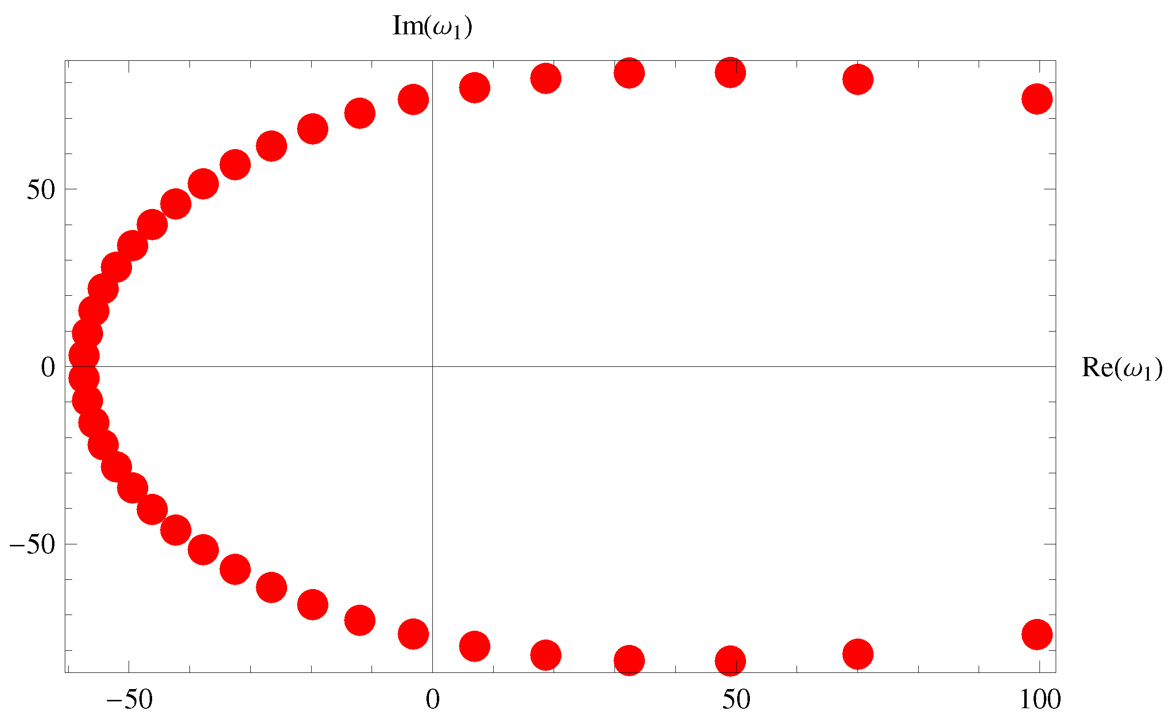
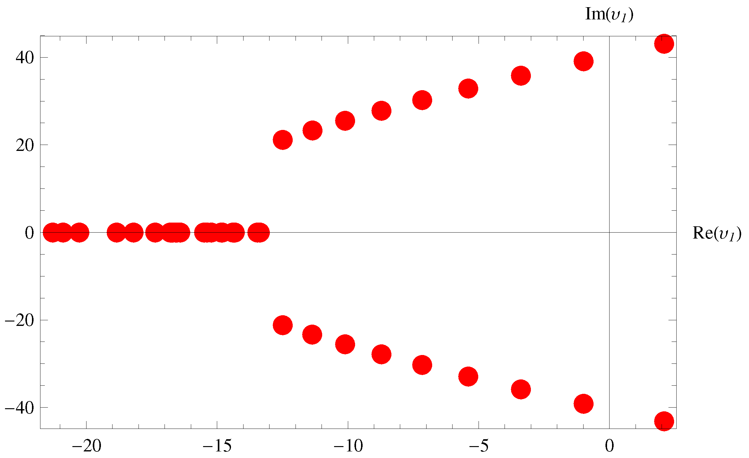
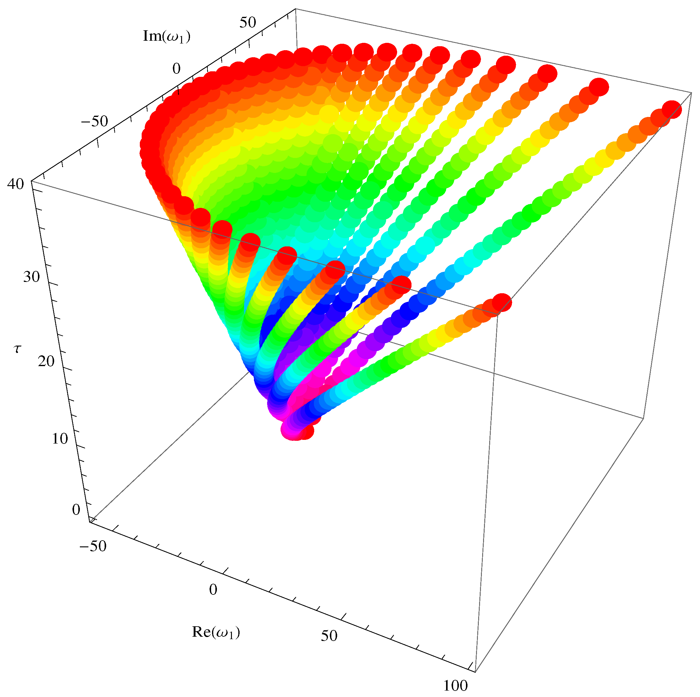
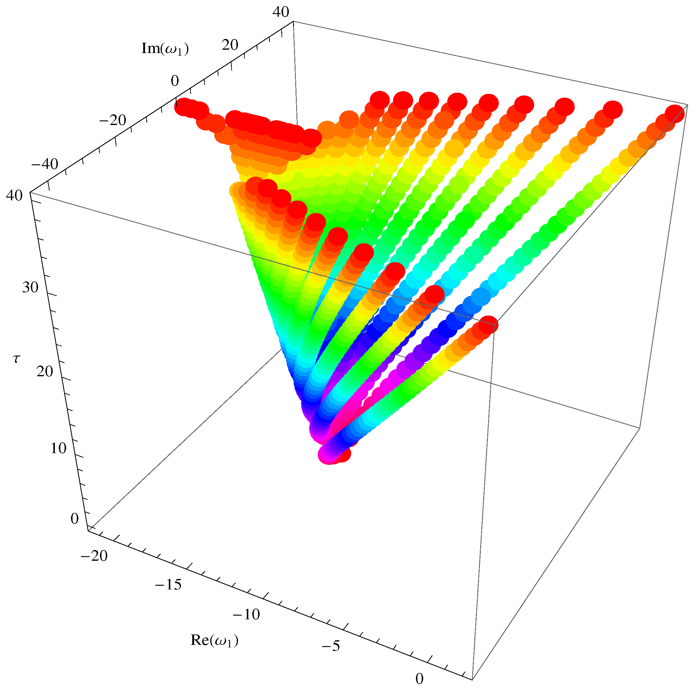
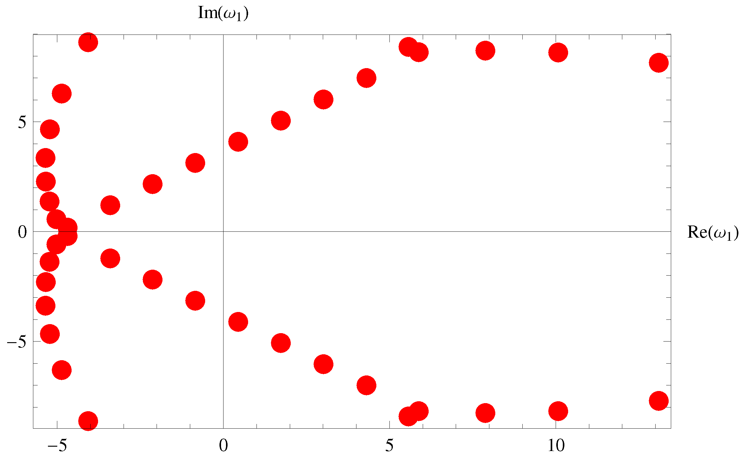
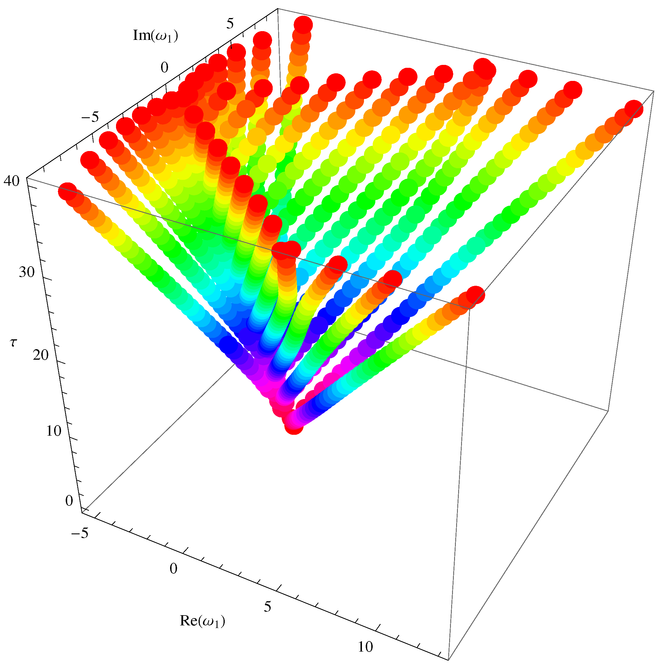
5. Special Members and Graphical Representations

Here, we acquire certain special hybrid members of the FBAP ${}_{\mathcal{F}\mathcal{B}el}\mathcal{A}_{\tau }^{\left(\sigma \right)}({\omega }_1,{\omega }_2,z)$. By leveraging the findings established in the earlier sections, we explore and analyze the results associated with these newly introduced special hybrid members.

5.1. Fubini–Bell-Based Bernoulli Polynomials

For $\mathcal{A}\left(\upsilon \right)={\displaystyle \frac{\upsilon }{e^{\upsilon }-1}}$, the FBAP ${}_{\mathcal{F}\mathcal{B}el}\mathcal{A}_{\tau }^{\left(\sigma \right)}({\omega }_1,{\omega }_2,z)$ (19) reduce to the Fubini–Bell-based Bernoulli polynomials (FBBP) ${}_{\mathcal{F}\mathcal{B}el}\mathcal{B}_{\tau }^{\left(\sigma \right)}({\omega }_1,{\omega }_2,z)$ which are expressed as follows:

$${\displaystyle \frac{\upsilon e^{{\omega }_1\upsilon +z(e^{\upsilon }-1)}}{\left(e^{\upsilon }-1\right){\left(1-{\omega }_2(e^{\upsilon }-1)\right)}^{\sigma }}}=\sum _{\tau =0}^{\infty }{}_{\mathcal{F}\mathcal{B}el}\mathcal{B}_{\tau }^{\left(\sigma \right)}({\omega }_1,{\omega }_2,z){\displaystyle \frac{{\upsilon }^{\tau }}{\tau !}}.$$

(59)

The FBBP ${}_{\mathcal{F}\mathcal{B}el}\mathcal{B}_{\tau }^{\left(\sigma \right)}({\omega }_1,{\omega }_2,z)$ satisfy the following representations:

$${}_{\mathcal{F}\mathcal{B}el}\mathcal{B}_{\tau }^{\left(\sigma \right)}({\omega }_1,{\omega }_2,z)=\sum _{\kappa =0}^{\tau }\left({\displaystyle \genfrac{}{}{0pt}{}{\tau }{\kappa }}\right){\mathcal{F}}_{\tau -\kappa }^{\left(\sigma \right)}\left({\omega }_2\right){}_{\mathcal{B}el}\mathcal{B}_{\kappa }({\omega }_1,z);$$

(60)

$${}_{\mathcal{F}\mathcal{B}el}\mathcal{B}_{\tau }^{\left(\sigma \right)}({\omega }_1,{\omega }_2,z)=\sum _{\kappa =0}^{\tau }\left({\displaystyle \genfrac{}{}{0pt}{}{\tau }{\kappa }}\right){}_{\mathcal{F}}\mathcal{B}e{l}_{\tau -\kappa }^{\left(\sigma \right)}({\omega }_2,z){\mathcal{B}}_{\kappa }\left({\omega }_1\right);$$

(61)

$${\omega }_2{}_{\mathcal{F}\mathcal{B}el}\mathcal{B}_{\tau }^{\left(\sigma \right)}({\omega }_1+1,{\omega }_2,z)=({\omega }_2+1){}_{\mathcal{F}\mathcal{B}el}\mathcal{B}_{\tau }^{\left(\sigma \right)}({\omega }_1,{\omega }_2,z)-{}_{\mathcal{F}\mathcal{B}el}\mathcal{B}_{\tau }^{(\sigma -1)}({\omega }_1,{\omega }_2,z).$$

(62)

For $\tau \in {\mathbb{N}}_0$ and $\sigma \in \mathbb{N}$, we have

$${}_{\mathcal{F}\mathcal{B}el}\mathcal{B}_{\tau }^{\left(\sigma \right)}({\omega }_1+\nu ,{\omega }_2,z)=\sum _{\kappa =0}^{\tau }\left({\displaystyle \genfrac{}{}{0pt}{}{\tau }{\kappa }}\right){}_{\mathcal{F}\mathcal{B}el}\mathcal{B}_{\kappa }^{\left(\sigma \right)}({\omega }_1,{\omega }_2,z){\nu }^{\tau -\kappa };$$

(63)

$${}_{\mathcal{F}\mathcal{B}el}\mathcal{B}_{\tau }^{(\sigma +\beta )}({\omega }_1+u,{\omega }_2,z+\rho )=\sum _{\kappa =0}^{\tau }\left({\displaystyle \genfrac{}{}{0pt}{}{\tau }{\kappa }}\right){}_{\mathcal{F}\mathcal{B}el}\mathcal{B}_{\kappa }^{\left(\sigma \right)}({\omega }_1,{\omega }_2,z){}_{\mathcal{F}\mathcal{B}el}\mathcal{B}_{\kappa }^{\left(\sigma \right)}e{l}_{\tau -\kappa }^{\left(\beta \right)}(u,{\omega }_2,\rho );$$

(64)

$${}_{\mathcal{F}\mathcal{B}el}\mathcal{B}_{\tau }^{(\sigma +1)}({\omega }_1,{\omega }_2,z)=\sum _{\kappa =0}^{\tau }\left({\displaystyle \genfrac{}{}{0pt}{}{\tau }{\kappa }}\right){}_{\mathcal{F}\mathcal{B}el}\mathcal{B}_{\kappa }^{\left(\sigma \right)}({\omega }_1,{\omega }_2,z){\mathcal{F}}_{\tau -\kappa }\left({\omega }_2\right);$$

(65)

$${}_{\mathcal{F}\mathcal{B}el}\mathcal{B}_{\tau }^{\left(\sigma \right)}({\omega }_1,{\omega }_2,z)={\displaystyle \frac{1}{2}}\sum _{\kappa =0}^{\tau }\left({\displaystyle \genfrac{}{}{0pt}{}{\tau }{\kappa }}\right)\left[{}_{\mathcal{F}\mathcal{B}el}\mathcal{B}_{\tau -\kappa }^{\left(\sigma \right)}({\omega }_1+1,{\omega }_2,z){\mathcal{E}}_{\kappa }+{}_{\mathcal{F}}\mathcal{B}_{\tau -\kappa }^{\left(\sigma \right)}\left({\omega }_2\right){}_{\mathcal{B}el}\mathcal{E}_{\kappa }({\omega }_1,z)\right].$$

(66)

For $\tau \in {\mathbb{N}}_0$ and $\sigma ,a,b\in \mathbb{N}$, the FBBP ${}_{\mathcal{F}\mathcal{B}el}\mathcal{B}_{\tau }^{\left(\sigma \right)}({\omega }_1,{\omega }_2,z)$ satisfy the following symmetry identities:

$$\begin{array}{cc}\hfill \sum _{\gamma =0}^{\tau }\left({\displaystyle \genfrac{}{}{0pt}{}{\tau }{\gamma }}\right)a^{\tau -\gamma }{b}^{\gamma }& {}_{\mathcal{F}\mathcal{B}el}\mathcal{B}_{\tau -\gamma }^{\left(\sigma \right)}(b{\omega }_1,{\omega }_2,z){}_{\mathcal{F}\mathcal{B}el}\mathcal{B}_{\gamma }^{\left(\sigma \right)}(a{\omega }_1,{\omega }_2,z)\hfill \\ & =\sum _{\gamma =0}^{\tau }\left({\displaystyle \genfrac{}{}{0pt}{}{\tau }{\gamma }}\right)b^{\tau -\gamma }{a}^{\gamma }{}_{\mathcal{F}\mathcal{B}el}\mathcal{B}_{\tau -\gamma }^{\left(\sigma \right)}(a{\omega }_1,{\omega }_2,z){}_{\mathcal{F}\mathcal{B}el}\mathcal{B}_{\gamma }^{\left(\sigma \right)}(b{\omega }_1,{\omega }_2,z).\hfill \end{array}$$

(67)

$$\begin{array}{cc}\hfill \sum _{\gamma =0}^{\tau }\sum _{\kappa =0}^{b-1}\sum _{\delta =0}^{a-1}& \left({\displaystyle \genfrac{}{}{0pt}{}{\tau }{\gamma }}\right)a^{\tau -\gamma }{b}^{\gamma }{}_{\mathcal{F}\mathcal{B}el}\mathcal{B}_{\tau -\gamma }^{\left(\sigma \right)}(b{\omega }_1+\kappa ,{\omega }_2,z){}_{\mathcal{F}\mathcal{B}el}\mathcal{B}_{\gamma }^{\left(\sigma \right)}(a{\omega }_1+\delta ,{\omega }_2,z)\hfill \\ & =\sum _{\gamma =0}^{\tau }\sum _{\kappa =0}^{a-1}\sum _{\delta =0}^{b-1}\left({\displaystyle \genfrac{}{}{0pt}{}{\tau }{\gamma }}\right)b^{\tau -\gamma }{a}^{\gamma }{}_{\mathcal{F}\mathcal{B}el}\mathcal{B}_{\tau -\gamma }^{\left(\sigma \right)}(a{\omega }_1+\kappa ,{\omega }_2,z){}_{\mathcal{F}\mathcal{B}el}\mathcal{B}_{\gamma }^{\left(\sigma \right)}(b{\omega }_1+\delta ,{\omega }_2,z).\hfill \end{array}$$

(68)

In [25], it was demonstrated that when ${\beta }_0=1$ and ${\beta }_j={\displaystyle \frac{1}{j+1}}$ for $j=1,2,3,\cdots ,\tau$, the determinant-based definition of Appell polynomials ${\mathcal{A}}_{\tau }\left({\omega }_1\right)$, as given by Equations (55) and (56), simplifies to the determinant-based definition of Bernoulli polynomials ${\mathcal{B}}_{\tau }\left({\omega }_1\right)$[24]. Consequently, by setting ${\beta }_0=1$ and ${\beta }_j={\displaystyle \frac{1}{j+1}}$ for $j=1,2,3,\cdots ,\tau$ in Equations (53) and (54), the following determinant representation of the FBBP ${}_{\mathcal{F}\mathcal{B}el}\mathcal{B}_{\tau }^{\left(\sigma \right)}({\omega }_1,{\omega }_2,z)$ is obtained.

Corollary 1.

The Fubini–Bell-based Bernoulli polynomials ${}_{\mathcal{F}\mathcal{B}el}\mathcal{B}_{\tau }^{\left(\sigma \right)}({\omega }_1,{\omega }_2,z)$ of degree τ are defined by

$$\begin{array}{c}\hfill {}_{\mathcal{F}\mathcal{B}el}\mathcal{B}_0^{\left(\sigma \right)}({\omega }_1,{\omega }_2,z)=1,\\ \hfill {}_{\mathcal{F}\mathcal{B}el}\mathcal{B}_{\tau }^{\left(\sigma \right)}({\omega }_1,{\omega }_2,z)\\ \hfill \begin{array}{c}\hfill ={(-1)}^{\tau }\left|\begin{array}{cccccc}1& {}_{\mathcal{F}}\mathcal{B}e{l}_1^{\left(\sigma \right)}({\omega }_1,{\omega }_2,z)& {}_{\mathcal{F}}\mathcal{B}e{l}_2^{\left(\sigma \right)}({\omega }_1,{\omega }_2,z)& ...& {}_{\mathcal{F}}\mathcal{B}e{l}_{\tau -1}^{\left(\sigma \right)}({\omega }_1,{\omega }_2,z)& {}_{\mathcal{F}}\mathcal{B}e{l}_{\tau }^{\left(\sigma \right)}({\omega }_1,{\omega }_2,z)\\ \\ 1& {\displaystyle \frac{1}{2}}& {\displaystyle \frac{1}{3}}& ...& {\displaystyle \frac{1}{\tau }}& {\displaystyle \frac{1}{\tau +1}}\\ \\ 0& 1& \left(\begin{array}{c}2\\ 1\end{array}\right){\displaystyle \frac{1}{2}}& ...& \left(\begin{array}{c}\tau -1\\ 1\end{array}\right){\displaystyle \frac{1}{\tau -1}}& \left(\begin{array}{c}\tau \\ 1\end{array}\right){\displaystyle \frac{1}{\tau }}\\ \\ 0& 0& 1& ...& \left(\begin{array}{c}\tau -1\\ 2\end{array}\right){\displaystyle \frac{1}{\tau -2}}& \left(\begin{array}{c}\tau \\ 2\end{array}\right){\displaystyle \frac{1}{\tau -1}}\\ .& .& .& ...& .& .\\ .& .& .& ...& .& .\\ 0& 0& 0& ...& 1& \left(\begin{array}{c}\tau \\ \tau -1\end{array}\right){\displaystyle \frac{1}{2}}\end{array}\right|\end{array},\\ \hfill \tau =1,2,3,...,\end{array}$$

(69)

where ${}_{\mathcal{F}}\mathcal{B}e{l}_{\tau }^{\left(\sigma \right)}({\omega }_1,{\omega }_2,z)(\tau =0,1,2,...)$ are the Fubini–Bell polynomials of degree τ.

The first four Fubini–Bell-based Bernoulli polynomials ${}_{\mathcal{F}\mathcal{B}el}\mathcal{B}_{\tau }^2({\omega }_1,{\omega }_2,z)$ are as follows:

$$\begin{array}{cc}\hfill & {}_{\mathcal{F}\mathcal{B}el}\mathcal{B}_0({\omega }_1,{\omega }_2,z)=1,\hfill \\ & {}_{\mathcal{F}\mathcal{B}el}\mathcal{B}_1({\omega }_1,{\omega }_2,z)=-{\displaystyle \frac{1}{2}}+{\omega }_1+{\omega }_2+z,\hfill \\ & {}_{\mathcal{F}\mathcal{B}el}\mathcal{B}_2({\omega }_1,{\omega }_2,z)={\displaystyle \frac{1}{6}}-{\omega }_1+{\omega }_1^2+2{\omega }_1{\omega }_2+2{\omega }_2^2+2{\omega }_{1}z+2{\omega }_{2}z+z^2,\hfill \\ & {}_{\mathcal{F}\mathcal{B}el}\mathcal{B}_3({\omega }_1,{\omega }_2,z)={\displaystyle \frac{{\omega }_1}{2}}-{\displaystyle \frac{3{\omega }_1^2}{2}}+{\omega }_1^3+3{\omega }_1^2{\omega }_2+3{\omega }_2^2+6{\omega }_1{\omega }_2^2+6{\omega }_2^3+3{\omega }_1^{2}z+3{\omega }_{2}z+6{\omega }_1{\omega }_{2}z\hfill \\ & +6{\omega }_2^{2}z+{\displaystyle \frac{3z^2}{2}}+3{\omega }_1{z}^2+3{\omega }_2{z}^2+z^3,\hfill \\ & {}_{\mathcal{F}\mathcal{B}el}\mathcal{B}_4({\omega }_1,{\omega }_2,z)={\displaystyle \frac{1}{30}}\left(-1+30{\omega }_1^2-60{\omega }_1^3+30{\omega }_1^4+120{\omega }_1^3{\omega }_2+120{\omega }_2^2+360{\omega }_1{\omega }_2^2+360{\omega }_1^2{\omega }_2^2\right.\hfill \\ & +720{\omega }_2^3+720{\omega }_1{\omega }_2^3+720{\omega }_2^4+120{\omega }_1^{3}z+120{\omega }_{2}z+360{\omega }_1{\omega }_{2}z+360{\omega }_1^2{\omega }_{2}z\hfill \\ & +720{\omega }_2^{2}z+720{\omega }_1{\omega }_2^{2}z+720{\omega }_2^{3}z+60z^2+180{\omega }_1{z}^2+180{\omega }_1^2{z}^2+360{\omega }_2{z}^2\hfill \\ & \left.+360{\omega }_1{\omega }_2{z}^2+360{\omega }_2^2{z}^2+120z^3+120{\omega }_1{z}^3+120{\omega }_2{z}^3+30z^4\right).\hfill \end{array}$$

Here also, we present the zero distributions of ${}_{\mathcal{F}\mathcal{B}el}\mathcal{B}_{40}^{\left(2\right)}({\omega }_1,{\omega }_2,z)=0$, for ${\omega }_2=3.5,z=7$ and ${\omega }_2={\displaystyle \frac{1}{4}},z=12$, in Figure 1 and Figure 2, respectively.

Furthermore, the 3D structure of zeros distributions of FBBP ${}_{\mathcal{F}\mathcal{B}el}\mathcal{B}_{\tau }^{\left(2\right)}({\omega }_1,{\omega }_2,z)=0$, $\tau =1,2,...,40$ for ${\omega }_2=3.5,z=7$ and ${\omega }_2={\displaystyle \frac{1}{4}},z=12$ are presented in Figure 3 and Figure 4, respectively.

5.2. Fubini–Bell-Based Euler Polynomials

For $\mathcal{A}\left(\upsilon \right)={\displaystyle \frac{2}{e^{\upsilon }+1}}$, the FBAP ${}_{\mathcal{F}\mathcal{B}el}\mathcal{A}_{\tau }^{\left(\sigma \right)}({\omega }_1,{\omega }_2,z)$ (19) simplifies to the Fubini–Bell-based Euler polynomials (FBEP) ${}_{\mathcal{F}\mathcal{B}el}\mathcal{E}_{\tau }^{\left(\sigma \right)}({\omega }_1,{\omega }_2,z)$, which are expressed as follows:

$${\displaystyle \frac{2e^{{\omega }_1\upsilon +z(e^{\upsilon }-1)}}{\left(e^{\upsilon }+1\right){\left(1-{\omega }_2(e^{\upsilon }-1)\right)}^{\sigma }}}=\sum _{\tau =0}^{\infty }{}_{\mathcal{F}\mathcal{B}el}\mathcal{E}_{\tau }^{\left(\sigma \right)}({\omega }_1,{\omega }_2,z){\displaystyle \frac{{\upsilon }^{\tau }}{\tau !}}.$$

(70)

The FBEP ${}_{\mathcal{F}\mathcal{B}el}\mathcal{E}_{\tau }^{\left(\sigma \right)}({\omega }_1,{\omega }_2,z)$ satisfy the following representations:

$${}_{\mathcal{F}\mathcal{B}el}\mathcal{E}_{\tau }^{\left(\sigma \right)}({\omega }_1,{\omega }_2,z)=\sum _{\kappa =0}^{\tau }\left({\displaystyle \genfrac{}{}{0pt}{}{\tau }{\kappa }}\right){\mathcal{F}}_{\tau -\kappa }^{\left(\sigma \right)}\left({\omega }_2\right){}_{\mathcal{B}el}\mathcal{E}_{\kappa }({\omega }_1,z);$$

(71)

$${}_{\mathcal{F}\mathcal{B}el}\mathcal{E}_{\tau }^{\left(\sigma \right)}({\omega }_1,{\omega }_2,z)=\sum _{\kappa =0}^{\tau }\left({\displaystyle \genfrac{}{}{0pt}{}{\tau }{\kappa }}\right){}_{\mathcal{F}}\mathcal{B}e{l}_{\tau -\kappa }^{\left(\sigma \right)}({\omega }_2,z){\mathcal{E}}_{\kappa }\left({\omega }_1\right);$$

(72)

$${\omega }_2{}_{\mathcal{F}\mathcal{B}el}\mathcal{E}_{\tau }^{\left(\sigma \right)}({\omega }_1+1,{\omega }_2,z)=({\omega }_2+1){}_{\mathcal{F}\mathcal{B}el}\mathcal{E}_{\tau }^{\left(\sigma \right)}({\omega }_1,{\omega }_2,z)-{}_{\mathcal{F}\mathcal{B}el}\mathcal{E}_{\tau }^{(\sigma -1)}({\omega }_1,{\omega }_2,z).$$

(73)

For $\tau \in {\mathbb{N}}_0$ and $\sigma \in \mathbb{N}$, we have

$${}_{\mathcal{F}\mathcal{B}el}\mathcal{E}_{\tau }^{\left(\sigma \right)}({\omega }_1+\nu ,{\omega }_2,z)=\sum _{\kappa =0}^{\tau }\left({\displaystyle \genfrac{}{}{0pt}{}{\tau }{\kappa }}\right){}_{\mathcal{F}\mathcal{B}el}\mathcal{E}_{\kappa }^{\left(\sigma \right)}({\omega }_1,{\omega }_2,z){\nu }^{\tau -\kappa };$$

(74)

$${}_{\mathcal{F}\mathcal{B}el}\mathcal{E}_{\tau }^{(\sigma +\beta )}({\omega }_1+u,{\omega }_2,z+\rho )=\sum _{\kappa =0}^{\tau }\left({\displaystyle \genfrac{}{}{0pt}{}{\tau }{\kappa }}\right){}_{\mathcal{F}\mathcal{B}el}\mathcal{E}_{\kappa }^{\left(\sigma \right)}({\omega }_1,{\omega }_2,z){}_{\mathcal{F}}\mathcal{B}e{l}_{\tau -\kappa }^{\left(\beta \right)}(u,{\omega }_2,\rho );$$

(75)

$${}_{\mathcal{F}\mathcal{B}el}\mathcal{E}_{\tau }^{(\sigma +1)}({\omega }_1,{\omega }_2,z)=\sum _{\kappa =0}^{\tau }\left({\displaystyle \genfrac{}{}{0pt}{}{\tau }{\kappa }}\right){}_{\mathcal{F}\mathcal{B}el}\mathcal{E}_{\kappa }^{\left(\sigma \right)}({\omega }_1,{\omega }_2,z){\mathcal{F}}_{\tau -\kappa }\left({\omega }_2\right);$$

(76)

$${}_{\mathcal{F}\mathcal{B}el}\mathcal{E}_{\tau }^{\left(\sigma \right)}({\omega }_1,{\omega }_2,z)={\displaystyle \frac{1}{2}}\sum _{\kappa =0}^{\tau }\left({\displaystyle \genfrac{}{}{0pt}{}{\tau }{\kappa }}\right)\left[{}_{\mathcal{F}\mathcal{B}el}\mathcal{E}_{\tau -\kappa }^{\left(\sigma \right)}({\omega }_1+1,{\omega }_2,z){\mathcal{E}}_{\kappa }+{}_{\mathcal{F}}\mathcal{E}_{\tau -\kappa }^{\left(\sigma \right)}\left({\omega }_2\right){}_{\mathcal{B}el}\mathcal{E}_{\kappa }({\omega }_1,z)\right].$$

(77)

For $\tau \in {\mathbb{N}}_0$ and $\sigma ,a,b\in \mathbb{N}$, the FBEP ${}_{\mathcal{F}\mathcal{B}el}\mathcal{E}_{\tau }^{\left(\sigma \right)}({\omega }_1,{\omega }_2,z)$ satisfy the following symmetry identities:

$$\begin{array}{cc}\hfill \sum _{\gamma =0}^{\tau }\left({\displaystyle \genfrac{}{}{0pt}{}{\tau }{\gamma }}\right)a^{\tau -\gamma }{b}^{\gamma }& {}_{\mathcal{F}\mathcal{B}el}\mathcal{E}_{\tau -\gamma }^{\left(\sigma \right)}(b{\omega }_1,{\omega }_2,z){}_{\mathcal{F}\mathcal{B}el}\mathcal{E}_{\gamma }^{\left(\sigma \right)}(a{\omega }_1,{\omega }_2,z)\hfill \\ & =\sum _{\gamma =0}^{\tau }\left({\displaystyle \genfrac{}{}{0pt}{}{\tau }{\gamma }}\right)b^{\tau -\gamma }{a}^{\gamma }{}_{\mathcal{F}\mathcal{B}el}\mathcal{E}_{\tau -\gamma }^{\left(\sigma \right)}(a{\omega }_1,{\omega }_2,z){}_{\mathcal{F}\mathcal{B}el}\mathcal{E}_{\gamma }^{\left(\sigma \right)}(b{\omega }_1,{\omega }_2,z).\hfill \end{array}$$

(78)

$$\begin{array}{cc}\hfill \sum _{\gamma =0}^{\tau }\sum _{\kappa =0}^{b-1}\sum _{\delta =0}^{a-1}& \left({\displaystyle \genfrac{}{}{0pt}{}{\tau }{\gamma }}\right)a^{\tau -\gamma }{b}^{\gamma }{}_{\mathcal{F}\mathcal{B}el}\mathcal{E}_{\tau -\gamma }^{\left(\sigma \right)}(b{\omega }_1+\kappa ,{\omega }_2,z){}_{\mathcal{F}\mathcal{B}el}\mathcal{E}_{\gamma }^{\left(\sigma \right)}(a{\omega }_1+\delta ,{\omega }_2,z)\hfill \\ & =\sum _{\gamma =0}^{\tau }\sum _{\kappa =0}^{a-1}\sum _{\delta =0}^{b-1}\left({\displaystyle \genfrac{}{}{0pt}{}{\tau }{\gamma }}\right)b^{\tau -\gamma }{a}^{\gamma }{}_{\mathcal{F}\mathcal{B}el}\mathcal{E}_{\tau -\gamma }^{\left(\sigma \right)}(a{\omega }_1+\kappa ,{\omega }_2,z){}_{\mathcal{F}\mathcal{B}el}\mathcal{E}_{\gamma }^{\left(\sigma \right)}(b{\omega }_1+\delta ,{\omega }_2,z).\hfill \end{array}$$

(79)

Moreover, when ${\beta }_0=1$ and ${\beta }_j={\displaystyle \frac{1}{2}}$ for $j=1,2,3,\dots ,\tau$, Equations (55) and (56) simplify to the determinant form of Euler polynomials ${\mathcal{E}}_{\tau }\left({\omega }_1\right)$[25]. Consequently, by setting ${\beta }_0=1$ and ${\beta }_j={\displaystyle \frac{1}{2}}$ for $j=1,2,3,\dots ,\tau$ in Equations (53) and (54), they reduce to the following determinant form of FBEP ${}_{\mathcal{F}\mathcal{B}el}\mathcal{E}_{\tau }^{\left(\sigma \right)}({\omega }_1,{\omega }_2,z)$.

Corollary 2.

The generalized Fubini–Bell-based Euler polynomials ${}_{\mathcal{F}\mathcal{B}el}\mathcal{E}_{\tau }^{\left(\sigma \right)}({\omega }_1,{\omega }_2,z)$ of degree τ are defined by

$$\begin{array}{c}\hfill {}_{\mathcal{F}\mathcal{B}el}\mathcal{E}_0^{\left(\sigma \right)}({\omega }_1,{\omega }_2,z)=1,\\ \hfill {}_{\mathcal{G}\mathcal{B}el}\mathcal{E}_{\tau }({\omega }_1,{\omega }_2,z)\end{array}$$

(80)

$$\begin{array}{c}\hfill \begin{array}{c}\hfill ={(-1)}^{\tau }\left|\begin{array}{cccccc}1& {}_{\mathcal{F}}\mathcal{B}e{l}_1^{\left(\sigma \right)}({\omega }_1,{\omega }_2,z)& {}_{\mathcal{F}}\mathcal{B}e{l}_2^{\left(\sigma \right)}({\omega }_1,{\omega }_2,z)& ...& {}_{\mathcal{F}}\mathcal{B}e{l}_{\tau -1}^{\left(\sigma \right)}({\omega }_1,{\omega }_2,z)& {}_{\mathcal{F}}\mathcal{B}e{l}_{\tau }^{\left(\sigma \right)}({\omega }_1,{\omega }_2,z)\\ \\ 1& {\displaystyle \frac{1}{2}}& {\displaystyle \frac{1}{2}}& ...& {\displaystyle \frac{1}{2}}& {\displaystyle \frac{1}{2}}\\ \\ 0& 1& \left(\begin{array}{c}2\\ 1\end{array}\right){\displaystyle \frac{1}{2}}& ...& \left(\begin{array}{c}\tau -1\\ 1\end{array}\right){\displaystyle \frac{1}{2}}& \left(\begin{array}{c}\tau \\ 1\end{array}\right){\displaystyle \frac{1}{2}}\\ \\ 0& 0& 1& ...& \left(\begin{array}{c}\tau -1\\ 2\end{array}\right){\displaystyle \frac{1}{2}}& \left(\begin{array}{c}\tau \\ 2\end{array}\right){\displaystyle \frac{1}{2}}\\ .& .& .& ...& .& .\\ .& .& .& ...& .& .\\ 0& 0& 0& ...& 1& \left(\begin{array}{c}\tau \\ \tau -1\end{array}\right){\displaystyle \frac{1}{2}}\end{array}\right|\end{array},\\ \hfill \tau =1,2,3,...,\end{array}$$

(81)

where ${}_{\mathcal{F}}\mathcal{B}e{l}_{\tau }^{\left(\sigma \right)}({\omega }_1,{\omega }_2,z)(\tau =0,1,2,...)$ are the Fubini–Bell polynomials of degree τ.

The first four Fubini–Bell-based Euler polynomials ${}_{\mathcal{F}\mathcal{B}el}\mathcal{E}_{\tau }({\omega }_1,{\omega }_2,z)$ are as follows:

$$\begin{array}{cc}\hfill & {}_{\mathcal{F}\mathcal{B}el}\mathcal{E}_0({\omega }_1,{\omega }_2,z)=1,\hfill \\ & {}_{\mathcal{F}\mathcal{B}el}\mathcal{E}_1({\omega }_1,{\omega }_2,z)=-{\displaystyle \frac{1}{2}}+{\omega }_1+{\omega }_2+z,\hfill \\ & {}_{\mathcal{F}\mathcal{B}el}\mathcal{E}_2({\omega }_1,{\omega }_2,z)=-{\omega }_1+{\omega }_1^2+2{\omega }_1{\omega }_2+2{\omega }_2^2+2{\omega }_{1}z+2{\omega }_{2}z+z^2,\hfill \\ & {}_{\mathcal{F}\mathcal{B}el}\mathcal{E}_3({\omega }_1,{\omega }_2,z)={\displaystyle \frac{1}{4}}\left(1-6{\omega }_1^2+4{\omega }_1^3-2{\omega }_2+12{\omega }_1^2{\omega }_2+12{\omega }_2^2+24{\omega }_1{\omega }_2^2+24{\omega }_2^3\right.\hfill \\ & \left.-2z+12{\omega }_1^{2}z+12{\omega }_{2}z+24{\omega }_1{\omega }_{2}z+24{\omega }_2^{2}z+6z^2+12{\omega }_1{z}^2+12{\omega }_2{z}^2+4z^3\right),\hfill \\ & {}_{\mathcal{F}\mathcal{B}el}\mathcal{E}_4({\omega }_1,{\omega }_2,z)=({\omega }_1-2{\omega }_1^3+{\omega }_1^4-2{\omega }_1{\omega }_2+4{\omega }_1^3{\omega }_2+2{\omega }_2^2+12{\omega }_1{\omega }_2^2+12{\omega }_1^2{\omega }_2^2+24{\omega }_2^3+24{\omega }_1{\omega }_2^3\hfill \\ & +24{\omega }_2^4-2{\omega }_{1}z+4{\omega }_1^{3}z+2{\omega }_{2}z+12{\omega }_1{\omega }_{2}z+12{\omega }_1^2{\omega }_{2}z+24{\omega }_2^{2}z+24{\omega }_1{\omega }_2^{2}z+24{\omega }_2^{3}z\hfill \\ & +z^2+6{\omega }_1{z}^2+6{\omega }_1^2{z}^2+12{\omega }_2{z}^2+12{\omega }_1{\omega }_2{z}^2+12{\omega }_2^2{z}^2+4z^3+4{\omega }_1{z}^3+4{\omega }_2{z}^3+z^4.\hfill \end{array}$$

Here also, we present the zero distributions of ${}_{\mathcal{F}\mathcal{B}el}\mathcal{E}_{40}^{\left(2\right)}({\omega }_1,{\omega }_2,z)=0$ for ${\omega }_2={\displaystyle \frac{1}{10}},$$z={\displaystyle \frac{1}{100}}$ and ${\omega }_2=-{\displaystyle \frac{1}{10}},z=-{\displaystyle \frac{1}{100}}$, in Figure 5 and Figure 6, respectively.

Furthermore, the 3D structure of zeros distributions of ${}_{\mathcal{F}\mathcal{B}el}\mathcal{E}_{\tau }^{\left(2\right)}({\omega }_1,{\omega }_2,z)=0$, $\tau =1,$$2,...,40$ for ${\omega }_2={\displaystyle \frac{1}{10}},z={\displaystyle \frac{1}{100}}$ and ${\omega }_2=-{\displaystyle \frac{1}{10}},z=-{\displaystyle \frac{1}{100}}$ are presented in Figure 7 and Figure 8, respectively.

Furthermore, by taking certain other choices of $\mathcal{A}\left(\upsilon \right)$, we can obtain some other special members of the Fubini–Bell-based Appell polynomials as follows:

• For $\mathcal{A}\left(\upsilon \right)={\displaystyle \frac{2\upsilon }{e^{\upsilon }+1}}$, the FBAP ${}_{\mathcal{F}\mathcal{B}el}\mathcal{A}_{\tau }^{\left(\sigma \right)}({\omega }_1,{\omega }_2,z)$ (19) reduce to the Fubini–Bell-based Genocchi polynomials, which are expressed as

  $${\displaystyle \frac{2\upsilon e^{{\omega }_1\upsilon +z(e^{\upsilon }-1)}}{\left(e^{\upsilon }+1\right){\left(1-{\omega }_2(e^{\upsilon }-1)\right)}^{\sigma }}}=\sum _{\tau =0}^{\infty }{}_{\mathcal{F}\mathcal{B}el}\mathcal{G}_{\tau }^{\left(\sigma \right)}({\omega }_1,{\omega }_2,z){\displaystyle \frac{{\upsilon }^{\tau }}{\tau !}}.$$

  (82)
• For $\mathcal{A}\left(\upsilon \right)={\displaystyle \frac{{\left(e^{\upsilon }-1\right)}^k}{k!}}$, the FBAP ${}_{\mathcal{F}\mathcal{B}el}\mathcal{A}_{\tau }^{\left(\sigma \right)}({\omega }_1,{\omega }_2,z)$ (19) reduce to the Fubini–Bell-based Stirling polynomials, which are expressed as

  $${\displaystyle \frac{{\left(e^{\upsilon }-1\right)}^k{e}^{{\omega }_1\upsilon +z(e^{\upsilon }-1)}}{k!{\left(1-{\omega }_2(e^{\upsilon }-1)\right)}^{\sigma }}}=\sum _{\tau =0}^{\infty }{}_{\mathcal{F}\mathcal{B}el}\mathcal{S}_2^{\left(\sigma \right)}(\tau ,k:{\omega }_1,{\omega }_2,z){\displaystyle \frac{{\upsilon }^{\tau }}{\tau !}}.$$

  (83)
• For $\mathcal{A}\left(\upsilon \right)={\left({\displaystyle \frac{2^{\varrho }{\upsilon }^{\mu }}{\lambda e^{\upsilon }+1}}\right)}^{\sigma }$, the FBAP ${}_{\mathcal{F}\mathcal{B}el}\mathcal{A}_{\tau }^{\left(\sigma \right)}({\omega }_1,{\omega }_2,z)$ (19) reduce to the Fubini–Bell-based Apostol-type polynomials, which are defined by

  $${\left({\displaystyle \frac{2^{\varrho }{\upsilon }^{\mu }}{(\lambda e^{\upsilon }+1)\left(1-{\omega }_2(e^{\upsilon }-1)\right)}}\right)}^{\sigma }{e}^{{\omega }_1\upsilon +z(e^{\upsilon }-1)}=\sum _{\tau =0}^{\infty }{}_{\mathcal{F}\mathcal{B}el}\mathcal{P}_{\tau }^{\left(\sigma \right)}({\omega }_1,{\omega }_2,z:\lambda ,\varrho ,\mu ){\displaystyle \frac{{\upsilon }^{\tau }}{\tau !}}.$$

  (84)
• For $\mathcal{A}\left(\upsilon \right)={\left({\displaystyle \frac{\upsilon }{\lambda e^{\upsilon }-1}}\right)}^{\sigma }$, the FBAP ${}_{\mathcal{F}\mathcal{B}el}\mathcal{A}_{\tau }^{\left(\sigma \right)}({\omega }_1,{\omega }_2,z)$ (19) reduce to the Fubini–Bell-based Apostol–Bernoulli polynomials, which are defined by

  $${\left({\displaystyle \frac{\upsilon }{(\lambda e^{\upsilon }-1)\left(1-{\omega }_2(e^{\upsilon }-1)\right)}}\right)}^{\sigma }{e}^{{\omega }_1\upsilon +z(e^{\upsilon }-1)}=\sum _{\tau =0}^{\infty }{}_{\mathcal{F}\mathcal{B}el}\mathcal{B}_{\tau }^{\left(\sigma \right)}({\omega }_1,{\omega }_2,z:\lambda ){\displaystyle \frac{{\upsilon }^{\tau }}{\tau !}}.$$

  (85)
• For $\mathcal{A}\left(\upsilon \right)={\left({\displaystyle \frac{2}{\lambda e^{\upsilon }+1}}\right)}^{\sigma }$, the FBAP ${}_{\mathcal{F}\mathcal{B}el}\mathcal{A}_{\tau }^{\left(\sigma \right)}({\omega }_1,{\omega }_2,z)$ (19) reduce to the Fubini–Bell-based Apostol–Euler polynomials, which are defined by

  $${\left({\displaystyle \frac{2}{(\lambda e^{\upsilon }+1)\left(1-{\omega }_2(e^{\upsilon }-1)\right)}}\right)}^{\sigma }{e}^{{\omega }_1\upsilon +z(e^{\upsilon }-1)}=\sum _{\tau =0}^{\infty }{}_{\mathcal{F}\mathcal{B}el}\mathcal{E}_{\tau }^{\left(\sigma \right)}({\omega }_1,{\omega }_2,z:\lambda ){\displaystyle \frac{{\upsilon }^{\tau }}{\tau !}}.$$

  (86)
• For $\mathcal{A}\left(\upsilon \right)={\left({\displaystyle \frac{2\upsilon }{\lambda e^{\upsilon }+1}}\right)}^{\sigma }$, the FBAP ${}_{\mathcal{F}\mathcal{B}el}\mathcal{A}_{\tau }^{\left(\sigma \right)}({\omega }_1,{\omega }_2,z)$ (19) reduce to the Fubini–Bell-based Apostol–Genocchi polynomials, which are defined by

  $${\left({\displaystyle \frac{2\upsilon }{(\lambda e^{\upsilon }+1)\left(1-{\omega }_2(e^{\upsilon }-1)\right)}}\right)}^{\sigma }{e}^{{\omega }_1\upsilon +z(e^{\upsilon }-1)}=\sum _{\tau =0}^{\infty }{}_{\mathcal{F}\mathcal{B}el}\mathcal{G}_{\tau }^{\left(\sigma \right)}({\omega }_1,{\omega }_2,z:\lambda ){\displaystyle \frac{{\upsilon }^{\tau }}{\tau !}}.$$

  (87)
• For $\mathcal{A}\left(\upsilon \right)={\left({\displaystyle \frac{1-u}{\lambda e^{\upsilon }-u}}\right)}^{\sigma }$, the FBAP ${}_{\mathcal{F}\mathcal{B}el}\mathcal{A}_{\tau }^{\left(\sigma \right)}({\omega }_1,{\omega }_2,z)$ (19) reduce to the Fubini–Bell-based Apostol-type Forbenius–Euler polynomials, which are defined by

  $${\left({\displaystyle \frac{1-u}{(\lambda e^{\upsilon }-u)\left(1-{\omega }_2(e^{\upsilon }-1)\right)}}\right)}^{\sigma }{e}^{{\omega }_1\upsilon +z(e^{\upsilon }-1)}=\sum _{\tau =0}^{\infty }{}_{\mathcal{F}\mathcal{B}el}\mathcal{H}_{\tau }^{\left(\sigma \right)}({\omega }_1,{\omega }_2,z:\lambda ,u){\displaystyle \frac{{\upsilon }^{\tau }}{\tau !}}.$$

  (88)

The series representations and other findings derived in the earlier sections can be utilized to explore the outcomes associated with the aforementioned special members.

6. Conclusions

The hybrid form of special polynomials and numbers has garnered considerable interest among researchers. In this study, we introduced a novel hybrid class of special polynomials, referred to as the Fubini–Bell-based Appell polynomials (FBAP). We explored their generating function and investigated several related properties. Symmetry identities involving the FBAP were also examined, and a determinant representation was derived. Specific members of the Fubini–Bell-based Appell family—such as the Fubini–Bell-based Bernoulli polynomials and the Fubini–Bell-based Euler polynomials—were obtained, with analogous results presented for each. Additionally, we analyzed computational outcomes and graphical representations of the zero distributions for these members. The method used in [36,37] can be considered in further studies. Future research could delve into the differential and integral representations of these special polynomials, as well as their potential applications.

References

1. Kargin, L. Some formulae for products of geometric polynomials with applications. J. Integer Seq. 2017, 20, 15. [Google Scholar]
2. Duran, U.; Acikgoz, M. Truncated Fubini polynomials. Mathematics 2019, 7, 431. [Google Scholar] [CrossRef]
3. Kim, D.S.; Kim, T.; Jang, G.-W. A note on degenerate Fubini polynomials. Proc. Jangjeon Math. Soc. 2017, 20, 521–531. [Google Scholar]
4. Kim, D.S.; Kim, T.; Kwon, H.I.; Park, J.W. Two variable higher-order Fubini polynomials. J. Korean Math. Soc. 2018, 55, 975–986. [Google Scholar] [CrossRef]
5. Kilar, N.; Simsek, Y. A new family of Fubini type numbers and polynomials associated with Apostol-Bernoulli numbers and polynomials. J. Korean Math. Soc. 2017, 54, 1605–1621. [Google Scholar]
6. Su, D.D.; He, Y. Some identities for the two variable Fubini polynomials. Mathematics 2019, 7, 115. [Google Scholar] [CrossRef]
7. Benbernou, S.; Gala, S.; Ragusa, M.A. On the regularity criteria for the 3D magnetohydrodynamic equations via two components in terms of BMO space. Math. Methods Appl. Sci. 2014, 37, 2320–2325. [Google Scholar] [CrossRef]
8. Boas, R.B.; Buck, R.C. Polynomial Expansions of Analytic Functions; Springer: Berlin/Heidelberg, Germany, 2013. [Google Scholar]
9. Sándor, J.; Crstici, B. Handbook of Number Theory; Kluwer Academic Publishers: Dordrecht, The Netherlands, 2004; Volume II. [Google Scholar]
10. Duran, U.; Araci, S.; Acikgoz, M. Bell-based Bernoulli polynomials with applications. Axioms 2021, 10, 29. [Google Scholar] [CrossRef]
11. Duran, U.; Acikgoz, M. Bell-based Genocchi polynomials. NTMSCI 2021, 9, 50–55. [Google Scholar] [CrossRef]
12. Carlitz, L. Some remarks on the Bell numbers. Fibonacci Quart. 1980, 18, 66–73. [Google Scholar] [CrossRef]
13. Al-Jawfi, R.A.; Muhyi, A.; Al-shameri, W.F.H. On generalized class of Bell polynomials associated with geometric applications. Axioms 2024, 13, 73. [Google Scholar] [CrossRef]
14. Costabile, F.A.; Khan, S.; Ali, H. A Study of the q-Truncated Exponential–Appell Polynomials. Mathematics 2024, 12, 3862. [Google Scholar] [CrossRef]
15. Muhyi, A.; Araci, S. A note on q-Fubini-Appell polynomials and related properties. J. Funct. Spaces 2022, 2021, 3805809. [Google Scholar] [CrossRef]
16. Srivastava, H.M.; Özarslan, M.A.; Yılmaz, B. Some families of differential equations associated with the Hermite-based Appell polynomials and other classes of Hermite-based polynomials. Filomat 2014, 28, 695–708. [Google Scholar] [CrossRef]
17. Özat, Z.; Özarslan, M.A.; Çekim, B. On Bell based Appell polynomials. Turk. J. Math. 2023, 47, 1099–1128. [Google Scholar] [CrossRef]
18. Avram, F.; Taqqu, M.S. Noncentral limit theorems and Appell polynomials. Ann. Probab. 1987, 15, 767–775. [Google Scholar] [CrossRef]
19. Andrews, L.C. Special Functions for Engineers and Applied Mathematics; Macmillan Publishing Company: New York, NY, USA, 1985. [Google Scholar]
20. Srivastava, H.M.; Manocha, H.L. A Treatise on Generating Functions; Halsted Press-Ellis Horwood Limited-John Wiley & Sons: New York, NY, USA, 1984. [Google Scholar]
21. Rainville, E.D. Special Functions; Chelsea Publishing Co.: Bronx, NY, USA, 1971. [Google Scholar]
22. Lu, D.Q.; Luo, Q.M. Some properties of the generalized Apostol type polynomials. Bound. Value Probl. 2013, 2013, 64. [Google Scholar] [CrossRef]
23. Kurt, B.; Simsek, Y. On the generalized Apostol-type Frobenius-Euler polynomials. Adv. Differ. Equ. 2013, 2013, 1–9. [Google Scholar] [CrossRef]
24. Costabile, F.A.; Dell’Accio, F.; Gualtieri, M.I. A new approach to Bernoulli polynomials. Rend. Mat. Appl. 2006, 26, 1–12. [Google Scholar]
25. Costabile, F.A.; Longo, E. A determinantal approach to Appell polynomials. J. Comput. Appl. Math. 2010, 234, 1528–1542. [Google Scholar] [CrossRef]
26. Costabile, F.A.; Longo, E. An algebraic approach to Sheffer polynomial sequences. Integral Transforms Spec. Funct. 2013, 25, 295–311. [Google Scholar] [CrossRef]
27. Cocolicchio, D.; Dattoli, G.; Srivastava, H.M. (Eds.) Advanced Special Functions and Applications; Aracne Editrice: Rome, Italy, 2000. [Google Scholar]
28. Muhyi, A. A new class of Gould-Hopper-Eulerian-type polynomials. Appl. Math. Sci. Eng. 2022, 30, 283–306. [Google Scholar] [CrossRef]
29. Ramírez, W.; Cesarano, C.; Wani, S.A.; Yousef, S.; Bedoya, D. About properties and the monomiality principle of Bell-based Apostol-Bernoulli-type polynomials. Carpathian Math. Publ. 2024, 16, 379–390. [Google Scholar] [CrossRef]
30. Srivastava, H.M.; Srivastava, R.; Muhyi, A.; Yasmin, G.; Islahi, H.; Araci, S. Construction of a new family of Fubini-type polynomials and its applications. Adv. Differ. Equ. 2021, 2021, 1–25. [Google Scholar] [CrossRef]
31. Srivastava, H.M.; Araci, S.; Khan, W.A.; Acikgoz, M. A note on the truncated-exponential based Apostol-type polynomials. Symmetry 2019, 11, 538. [Google Scholar] [CrossRef]
32. Yasmin, G.; Muhyi, A. Extended forms of Legendre-Gould-Hopper-Appell polynomials. Adv. Stud. Contemp. Math. 2019, 29, 489–504. [Google Scholar]
33. Masjed-Jamei, M.; Beyki, M.R.; Koepf, W. A new type of Euler polynomials and numbers. Mediterr. J. Math. 2018, 15, 138. [Google Scholar] [CrossRef]
34. Steffensen, J.F. The poweriod, an extension of the mathematical notion of power. Acta Math. 1941, 73, 333–366. [Google Scholar] [CrossRef]
35. Khan, N.; Husain, S. Analysis of Bell based Euler polynomials and their application. Int. J. Appl. Comput. Math. 2021, 7, 195. [Google Scholar] [CrossRef]
36. Lyapin, A.P.; Akhtamova, S.S. Recurrence relations for the sections of the generating series of the solution to the multidimensional difference equation. Vestn. Udmurtsk. Univ. Mat. Mekh. 2021, 31, 414–423. [Google Scholar] [CrossRef]
37. Leinartas, E.; Shishkina, O. The Euler-Maclaurin Formula in the Problem of Summation over Lattice Points of a Simplex. J. Sib. Fed. Univ. Math. Phys. 2022, 15, 108–113. [Google Scholar] [CrossRef]
Figure 1. Zeros of B 40 ( 2 ) F B e l ( ω 1 , 3.5 , 7 ) = 0 .
Mathematics 13 01009 g001
Figure 2. Zeros of B 40 ( 2 ) F B e l ( ω 1 , 1 4 , 12 ) = 0 .
Mathematics 13 01009 g002
Figure 3. Zero distribution of B τ ( 2 ) F B e l ( ω 1 , 3.5 , 7 ) = 0 . This figure illustrates the 3D plot of the zeros of Fubini–Bell-based Bernoulli polynomials B τ ( 2 ) F B e l ( ω 1 , ω 2 , z ) = 0 for τ = 1 , 2 , . . . , 40 , and ω 2 = 3.5 , z = 7 .
Mathematics 13 01009 g003
Figure 4. Zero distribution of B τ ( 2 ) F B e l ( ω 1 , 1 4 , 12 ) = 0 . This figure illustrates the 3D plot of the zeros of Fubini–Bell-based Bernoulli polynomials B τ ( 2 ) F B e l ( ω 1 , ω 2 , z ) = 0 for τ = 1 , 2 , . . . , 40 , and ω 2 = 1 4 , z = 12 .
Mathematics 13 01009 g004
Figure 5. Zeros of B 40 ( 2 ) F B e l ( ω 1 , 1 10 , 1 100 ) = 0 .
Mathematics 13 01009 g005
Figure 6. Zeros of B 40 ( 2 ) F B e l ( ω 1 , 1 10 , 1 100 ) = 0 .
Mathematics 13 01009 g006
Figure 7. Zero distribution of E τ ( 2 ) F B e l ( ω 1 , 1 10 , 1 100 ) = 0 . This figure illustrates the 3D plot of the zeros of Fubini–Bell-based Euler polynomials B τ ( 2 ) F B e l ( ω 1 , ω 2 , z ) = 0 for τ = 1 , 2 , . . . , 40 , and ω 2 = 1 10 , z = 1 100 .
Mathematics 13 01009 g007
Figure 8. Zero distribution of E τ ( 2 ) F B e l ( ω 1 , 1 10 , 1 100 ) = 0 . This figure illustrates the 3D plot of the zeros of Fubini–Bell-based Euler polynomials E τ ( 2 ) F B e l ( ω 1 , ω 2 , z ) = 0 for τ = 1 , 2 , . . . , 40 , and ω 2 = 1 10 , z = 1 100 .
Mathematics 13 01009 g008