Abstract
The quality of the processed products in CNC machining centers is a critical factor in manufacturing equipment. The anomaly detection and predictive maintenance functions are essential for improving efficiency and reducing time and costs. This study aims to strengthen service competitiveness by reducing quality assurance costs and implementing AI-based predictive maintenance services, as well as establishing a predictive maintenance system for CNC manufacturing equipment. The proposed system integrates preventive maintenance, time-based maintenance, and condition-based maintenance strategies. Using continuous learning based on long short-term memory (LSTM), the system enables anomaly detection, failure prediction, cause analysis, root cause identification, remaining useful life (RUL) prediction, and optimal maintenance timing decisions. In addition, this study focuses on roller-cutting devices that are essential in packaging processes, such as food, pharmaceutical, and cosmetic production. When rolling pins are machining with CNC equipment, a sensor system is installed to collect acoustic data, analyze failure patterns, and apply RUL prediction algorithms. The AI-based predictive maintenance system developed ensures the reliability and operational efficiency of CNC equipment, while also laying the foundation for a smart factory monitoring platform, thus enhancing competitiveness in intelligent manufacturing environments.
MSC:
26-04; 68T01
1. Introduction
Computerized Numerical Control (CNC) machining centers [1] have become essential equipment in modern manufacturing, performing precise machining operations with high accuracy and productivity. These machines require reliable operation, and the importance of maintenance strategies has been increasingly emphasized. In particular, in intelligent manufacturing environments such as smart factories, the early detection of anomalies, fault prediction, and the implementation of efficient maintenance strategies are crucial.
To explain more specifically the impact of various factors on the results in CNC machining, several elements such as the material’s mechanical properties, cutting speed, tool shape, and whether cutting fluid is used play significant roles. Materials with high hardness accelerate tool wear, affecting cutting quality, and if the cutting speed is too high, increased heat generation can shorten tool life and degrade surface roughness. In our study, we extracted these characteristics and collected and labeled data on the characteristic sound generated when a machining press molds materials (SKD-11) [2,3] through field engineers, utilizing field experience data.
Previous studies have focused on condition-based maintenance (CBM) [4,5] and time series data analysis to monitor equipment conditions and detect anomalies. The advent of deep learning techniques, such as long short-term memory (LSTM) [6,7] networks, has significantly improved the precision of time series data processing for maintenance. Recently, unsupervised learning methods like AnoGAN (Anomaly Detection using Generative Adversarial Networks) [8,9,10,11] have been introduced, minimizing human intervention and advancing automated maintenance systems.
Despite these advancements, several challenges remain: (1) Most existing algorithms require data preprocessing, which necessitates additional time and user intervention in processing raw data. (2) Current CBM approaches face limitations in accurately predicting equipment failures, lacking effective optimization models for predictive maintenance. (3) The usage of other forms of manufacturing data, such as acoustic data, remains inadequately analyzed and used. (4) Existing maintenance systems struggle to integrate seamlessly with smart-factory platforms, reducing their competitiveness in intelligent manufacturing environments.
LSTM excels at learning time series patterns but lacks reconstruction-based anomaly detection, relying solely on prediction errors. In contrast, f-AnoGAN [12] leverages GAN-based [13] learning to detect anomalies using reconstruction errors and the discriminator’s judgment, enabling efficient detection with limited data. However, it does not capture temporal dependencies. Combining LSTM with f-AnoGAN enhances anomaly detection by learning sequential patterns, allowing for more precise anomaly identification. This approach integrates LSTM’s prediction error, f-AnoGAN’s reconstruction error, and the discriminator’s judgment, strengthening the anomaly detection criteria for improved accuracy.
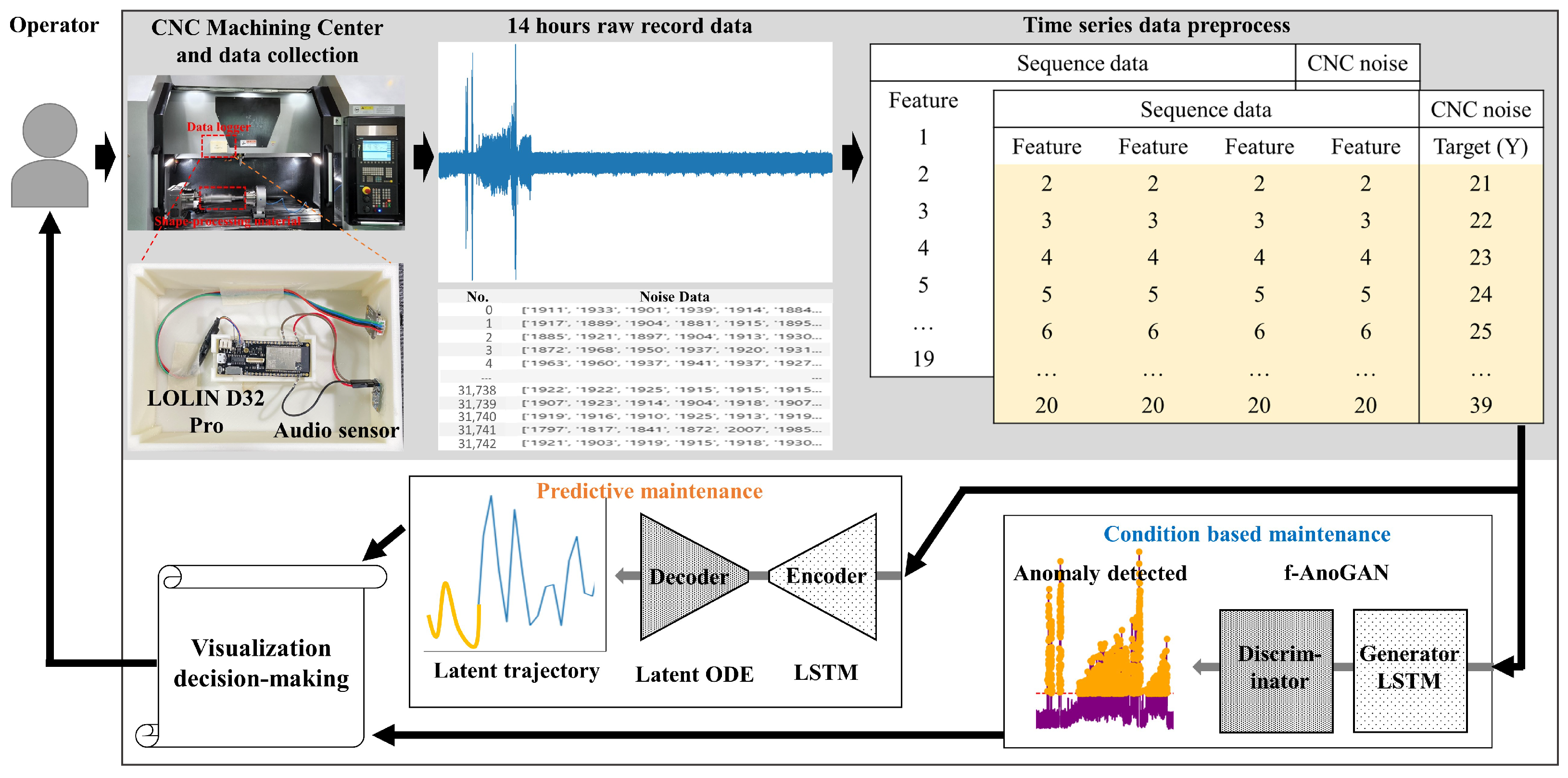
To address these issues, this study proposes the following innovative approaches: An AI-based predictive maintenance framework was developed to enhance the reliability and operational efficiency of CNC machining centers. An LSTM+latent ODE [11,14,15] algorithm was designed that goes beyond CBM to optimize predictive maintenance for time series data. On top of that, a fully unsupervised anomaly detection method was implemented using LSTM+f-AnoGAN [12,16] algorithms, enabling complete automation with raw data and no preprocessing, followed by a fault pattern analysis and remaining useful life (RUL) [17,18] prediction algorithms using acoustic data from CNC-processed roller-cutting workpieces. In addition, we integrated predictive maintenance capabilities into a smart factory’s monitoring platform, strengthening intelligent manufacturing competitiveness. The findings of this research are expected to significantly contribute to the advancement of intelligent maintenance systems in manufacturing environments while enhancing the competitiveness of smart factories. Figure 1 presents the workflow that we have developed.

Figure 1.
The sound sensor (raw data) was measured every 50 ms and had 1 s of data for each row. Using unsupervised learning with condition-based maintenance (CBM) and LSTM, we analyzed the temporal patterns of anomalies to perform anomaly detection (f-AnoGAN) and determine the anomaly status of machine conditions. When anomalies were detected, the information was visualized and forwarded to the decision-making module. To predict data for predictive maintenance (PdM), an LSTM network was utilized to estimate the latent trajectory of the system based on time series data derived from latent ODEs. This step predicted the future operational states of the machine based on its normal condition. Based on the information generated in these two stages, operators can understand the current state of the machine and assess future risks through visualized data, enabling them to decide on appropriate maintenance actions.
The key contributions of this study are as follows:
- We developed an AI-based anomaly detection method and predictive maintenance framework to enhance the reliability and operational efficiency of CNC machining centers.
- An LSTM+latent ODE algorithm was proposed to optimize predictive maintenance, going beyond traditional condition-based maintenance for time series data.
- A fully unsupervised anomaly detection method was implemented using LSTM+f-AnoGAN algorithms, enabling automated detection and diagnosis without user intervention by utilizing raw data without preprocessing.
- An analysis of failure patterns and a prediction algorithm using acoustic data from CNC machining equipment for roller-blade processing were implemented.
- The predictive maintenance capabilities were integrated into a smart factory’s monitoring platform, strengthening intelligent manufacturing competitiveness.
2. Related Work
Maintenance methods in smart factories can be broadly classified into reactive maintenance and preventive maintenance. Reactive maintenance involves repairing equipment after a failure has occurred. While it has lower initial maintenance costs, it can lead to unexpected downtime, reduced productivity, and increased operational expenses. On the other hand, preventive maintenance aims to prevent equipment failures in advance. It is further divided into time-based maintenance, condition-based maintenance, and predictive maintenance.
2.1. Time-Based Maintenance
This method involves conducting regular inspections and replacing parts based on fixed time intervals (e.g., usage hours, operational cycles). It is a preventive maintenance approach where regular inspections and maintenance are performed to prevent equipment or system failures [5,19,20]. Actions are taken based on a fixed inspection cycle, with the primary focus on reducing the risk of breakdowns. Preventive maintenance can extend the lifespan of equipment, prevent unexpected failures, and reduce long-term maintenance costs. However, the initial costs may be higher due to the regular and fixed nature of the maintenance.
In addition, corrective maintenance is a repair strategy implemented after a breakdown. It is a reactive approach that responds only when a failure occurs. The primary drawback of this method is its 100% failure risk, as actions are only taken after the breakdown. This can lead to exorbitant maintenance costs. Reactive maintenance is often used for urgent repairs, but it can also result in unexpected downtime and high repair costs.
2.2. Condition-Based Maintenance
Condition-based maintenance (CBM) [11,21,22] is a strategy that involves monitoring the condition of equipment or systems and making maintenance decisions based on the collected signals and data. This approach continuously monitors the condition of equipment to reduce the risk of failure and performs maintenance only when necessary, thereby reducing maintenance costs. By detecting signs of failure before they occur, CBM [23] allows for proactive measures, increasing equipment uptime and minimizing unexpected downtime.
By analyzing various signals and data (such as vibration, temperature, pressure, etc.) that indicate the condition of the equipment, the likelihood of failure can be predicted, and maintenance tasks can be performed based on this analysis, reducing the risk of failure. This also helps to minimize unnecessary preventive maintenance and reduce maintenance costs by replacing only the necessary parts when a failure occurs. Furthermore, by minimizing production disruptions caused by unexpected equipment failures, productivity is improved, and the equipment’s lifespan is extended by accurately assessing and managing its condition.
2.3. Predictive Maintenance
Predictive maintenance (PdM) [24,25,26] is a technique that monitors the condition of CNC machining centers to predict potential failures and take preventive measures. By implementing PdM, it is possible to prevent up to 70% of system failures and reduce unnecessary maintenance costs by approximately one-third. In particular, the use of AI techniques like LSTM can reduce reliance on expert engineers and expand the market for PdM [27,28,29,30] solutions.
However, PdM faces several challenges, including the need for vast quantities of data, the analysis of fault mechanisms, and the development of solutions for anomalies. Additionally, it requires highly skilled experts and significant investment in technology.
In conclusion, while PdM is an effective method to increase equipment uptime and reduce costs, successful implementation requires data analysis capabilities, skilled personnel, and appropriate technology investment. Companies should carefully evaluate the pros and cons of PdM and develop optimal strategies tailored to their specific environments.
To address these issues, we used a residual analysis technique among anomaly detection methods to create a model that predicts normal behavior. By analyzing the difference (residual) between the actual observations and the values predicted by the model, we detected anomalous states. Additionally, by combining machine learning and deep learning-based anomaly detection technologies (such as f-AnoGAN, LSTM-based models, latent ODE, etc.), a more sophisticated analysis became possible.
In CNC machining [31,32], various factors influence the results, with key variables including the material’s mechanical properties, cutting speed, tool geometry, and the use of cutting fluid. Harder materials accelerate tool wear, affecting cutting quality, while excessively high cutting speeds increase heat generation, leading to reduced tool life and deteriorated surface roughness [33,34]. In this study, we analyzed these characteristics by collecting and labeling data on the characteristic sounds generated during the machining of press mold material (SKD-11) through field engineers, utilizing field experience data.
2.4. General Framework
Variational Autoencoders (VAEs) [35,36,37] are a type of generative model that learn to model the distribution of data and generate new samples from that distribution. They extend the basic Autoencoder (AE) [38,39] concept by incorporating probabilistic elements to create a more flexible and powerful generative model.
A VAE can generate new data by sampling from the latent space and has stronger generalization capabilities by modeling the probabilistic distribution of the data. It effectively captures the complex structure of the data and can model a variety of distributions. Due to these advantages, VAEs are widely used in various fields, such as image generation, data augmentation, and anomaly detection.
An LSTM network is used for handling sequential data and learning patterns over time, such as time series forecasting or sequence classification. The LSTM network calculates the output for a given input sequence as follows:
Here, is the output of the LSTM network at time step t, and is the input sequence data. This output captures important temporal patterns from the sequence.
f-AnoGAN [40] is an anomaly detection model based on a GAN that learns the distribution of normal data and detects anomalies by comparing new data to this distribution. f-AnoGAN consists of a generator G, a discriminator D, and an encoder E. The generator creates fake data that mimic normal data, the discriminator classifies the data as real or fake, and the encoder maps input data to the latent space for faster anomaly detection (Equation (2)).
where z is the latent vector, are the parameters of the generator, and is the generated data (Equation (2)).
The encoder E maps input data x to the latent space z, where denotes the parameters of the encoder (Equation (3)).
The discriminator D represents the probability that the data x are real (normal), and is the sigmoid activation function (Equation (4)).
The key difference in f-AnoGAN is the introduction of an encoder, which efficiently calculates the latent vector of new data. Anomalies are detected based on the distance in the latent space and reconstruction error.
A Variational Autoencoder (VAE) compresses input data x into a latent space representation z and reconstructs it back to its original space.
The encoder transforms the input x from a high-dimensional space to a lower-dimensional latent space z, estimating the mean () and variance () of the latent variable z:
To sample the latent variable z, the reparameterization trick is applied to ensure the sampling process is differentiable:
where , and I is the identity matrix.
The decoder reconstructs the original input from the latent variable z:
The VAE loss consists of two components: the reconstruction loss and the KL divergence loss:
The overall loss is given by .
A latent ODE models the latent variable z as a continuous trajectory over time using ordinary differential equations (ODEs).
The change in the latent state over time is modeled using an ODE function:
where is a neural network consisting of a Tanh activation function and linear transformations:
Given the initial state and a time range t, the ODE is solved as:
Here, ODEINT is a numerical solver that computes the latent state over time. The trajectory of over time is plotted to visualize the evolution of the latent space.
3. Proposed Model
3.1. State-Based Anomaly Detection Method
LSTM+f-AnoGAN combined: The LSTM network processes sequential data and extracts features, while f-AnoGAN detects anomalies in these features using an encoder, generator, and discriminator. The output of the LSTM network is passed to f-AnoGAN for anomaly detection. First, the sequential data are passed through the LSTM network to produce the output :
This is then mapped to the latent space z using the encoder E:
The latent vector z is input to the f-AnoGAN’s generator G to generate a normal pattern:
The generated is evaluated by the discriminator D:
The encoder, generator, and discriminator work together to detect anomalies. Anomalies are identified based on the distance between and as well as the output of the discriminator D. This combined model enhances anomaly detection in sequential data by leveraging LSTM’s feature extraction and f-AnoGAN’s efficient anomaly scoring.
The LSTM loss function is defined based on the difference between the predicted and actual values:
Here, is the actual value, and is the predicted value.
The f-AnoGAN loss function combines reconstruction loss and feature mapping loss:
where is the reconstruction loss, measuring the difference between the input and the generator output . is the feature mapping loss, evaluating the difference in discriminator feature representations between the input and the generated output . is a hyperparameter that balances the two loss terms.
The total loss function for the combined model can be written as:
where is a hyperparameter that balances the importance of the two loss terms.
The LSTM network processes sequential data and extracts meaningful temporal features, while f-AnoGAN combines reconstruction loss and feature mapping loss to detect anomalies. The combined model uses the LSTM output to generate normal data with the f-AnoGAN generator, and the discriminator evaluates the anomaly score of these generated data. This approach enhances anomaly detection performance in time series data by leveraging the temporal pattern recognition of LSTM and the advanced anomaly detection capabilities of f-AnoGAN. The LSTM network learns time-dependent features, and unlike the original f-AnoGAN, which analyzes individual samples, it learns the normal flow in continuous time-series patterns and can detect anomalies by setting thresholds based on this learning.
3.2. Prediction-Based Detection Methods
Combining latent ODEs, a VAE, and LSTM networks involves using a Variational Autoencoder (VAE) to encode observations into a latent probabilistic space, latent ODEs to model continuous latent dynamics, and LSTM networks to refine the states with discrete sequential observations. Below is the mathematical representation of the process.
- Combining VAE, latent ODEs, and LSTM
The combination of VAE, latent ODE, and LSTM involves the following steps:
- -
- Latent state initialization: encode the input data into the latent probabilistic space using the VAE encoder:
- -
- Continuous state modeling: use latent ODEs to predict the continuous latent state:
- -
- State update with LSTM: update the state using LSTM with the observation and the latent state :
- -
- Reinitialize latent state: map the LSTM output back to the latent space for the next ODE step:
- Final Mathematical Formulation
The combined process can be summarized as follows:
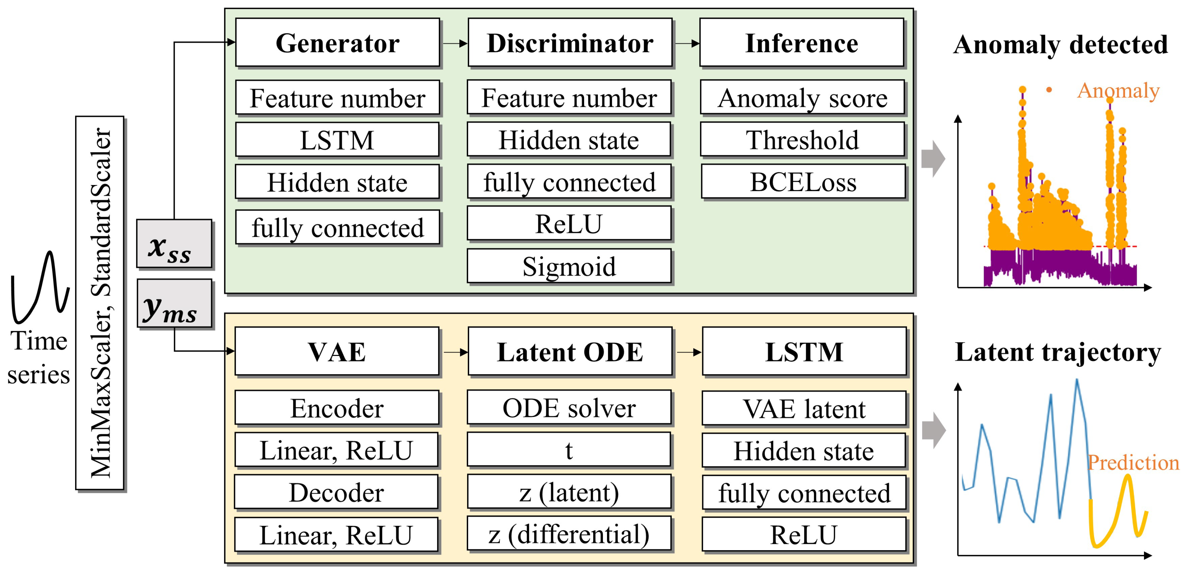
This hybrid approach enables probabilistic modeling of latent states (via the VAE), continuous time dynamics (via latent ODEs), and discrete time series updates (via LSTM). It enhances the detection of anomalies in irregularly sampled time series data by leveraging the strengths of each component. Figure 2 shows the overall process of the model we designed, presented step by step.
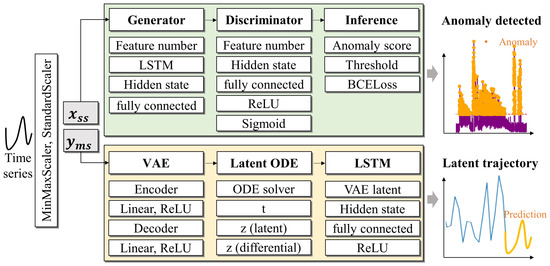
Figure 2.
This is a model for anomaly detection in time series data. After performing data preprocessing using techniques such as MinMaxScaler and StandardScaler, the LSTM× f-AnoGAN learns and generates features of the time series data, calculates anomaly scores based on the discriminator’s judgment, and detects anomalies when the score exceeds a threshold. The LSTM× latent ODE model compresses and reconstructs VAE time series data into a low-dimensional latent space, while modeling data changes within the latent ODE’s latent space. In the LSTM layer, the future of the time series data is predicted based on the results of the latent ODE. Finally, anomalies are detected, and data changes are visualized.
4. Experiments
This section describes the overall design of the experimental setup for the CNC equipment used in this study, focusing on the installation of factory devices and sensor nodes. We designed experiments to answer the following questions:
Anomaly detection accuracy: How accurately can the LSTM-based f-AnoGAN, trained in an unsupervised manner without preprocessing, distinguish between normal and abnormal data by setting a threshold (operating threshold)?
Anomaly prediction accuracy: In time series data without preprocessing and labels, how well can the LSTM-based latent ODE identify and predict abnormal segments?
Verification of model generalization: Do the f-AnoGAN combined with LSTM and latent ODE (VAE) models successfully detect anomalies in the Yahoo Anomaly Dataset?
4.1. Data Collection
Sensor node setup. To collect real-time data from the CNC machining process, a sensor node was designed and implemented using the following components:
- Microcontroller board: A LOLIN D32 (Arduino IDE 2.0) Pro [41] board was utilized to handle data acquisition and processing.
- Microphone sensor: A MAX4466 (Adafruit, Brooklyn, NY, USA) microphone sensor was employed to collect acoustic signals, specifically focusing on noise generated during the machining process. Designed by Analog Devices and manufactured in China.
Material specifications and machining details. For the experiments, shaping and processing were performed on SKD 11 material with the following specifications:
- Material: high-strength steel (SKD 11) [42] commonly used in industrial applications.
- Dimensions: the material block measured 300 × 115 mm.
- Machining time: the total machining process spanned 48 h, including 7∼8 h for drilling operations.
- Drilling details: number of drills used: 1∼2 tungsten carbide end mills (typically 1).
- Drill specifications: tungsten carbide end mill with a diameter of 10 mm and a corner radius of 1 mm.
Power supply. The sensor node and logging system were powered using the following:
- Battery pack: a 1000 mAh battery connected to the LOLIN D32 Pro board.
- Operating current: the setup consumed approximately 700 mA during operation.
Data logger operation: to ensure continuous data recording, the data logger was designed to operate for 14 h per session, allowing for extended monitoring of the machining process without interruptions.
Edge server setup: For temporary data storage and transmission within the factory, the Nvidia Jetson Xavier was used as the server, which could be replaced with a Jetson Nano or Raspberry Pi. The edge server received sensor data via BLE and transmitted data to the main server using Wi-Fi or LTE-M.
Main server setup: For data transmission and database management, a cloud server (OCI or AWS) was used. Additionally, an SSL certificate issuance and automatic renewal system was implemented to enable HTTPS security. A time series database was set up to store sensor data, and data reception and transmission features were provided via a RESTful API service. InfluxDB was used to store sensor data, and OracleDB was used to manage authentication data.
Noise data collection results: The sound sensor measured data at 50 ms intervals, with each row containing one second of data. Each data row followed the structure shown below in Figure 3, which also displays the result of its visualization. Table 1 provides information about the CNC noise dataset used in this experiment.
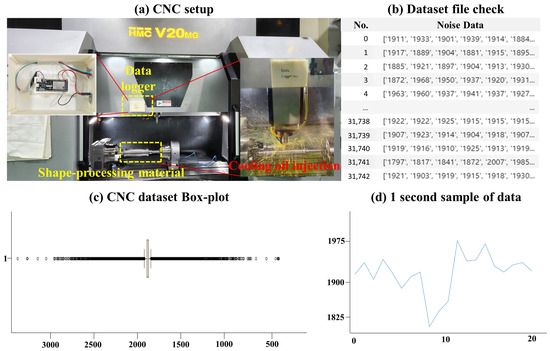
Figure 3.
(a) Internal view of the data logger installed in the actual CNC equipment and the coolant oil being sprayed during the shaping process. In (b,c), the data structure can be analyzed using a box plot, and (d) presents the visualization of data over a one-second period.

Table 1.
Information about the CNC Noise Dataset used in this experiment. The dataset size is the sum of the number of rows and columns, and the anomaly section is approximately between 13,000 and 45,000. *: information about the Yahoo Anomaly Dataset.
This overall design enabled effective data acquisition and analysis, providing a robust foundation for anomaly detection and predictive maintenance experiments in CNC machining environments.
Additionally, while this study focused on an AI-based analysis, we also explored a method that could be implemented in real-time systems. Two approaches were used for applying it in a real-time system. The first was to implement it directly on an edge server, enabling real-time push notifications and monitoring for users. The second approach involved training the model on a high-performance computer in a cloud server and then delivering the results to users. Sensor data collected in real time by the data logger were stored through a buffer set with a transmission speed of 4 ms, and the storage duration could be adjusted between 1 and 3 s. The stored data were then sequentially fed into the LSTM+f-AnoGAN model. Another approach was to apply an algorithm that analyzed the MinMax cycle of a specific signal instead of storing data based on time, allowing only characteristic signals to be stored from the start to the end point. The combination of the LSTM+f-AnoGAN model integrated time-based storage methods with AI applications, while the LSTM+latent ODE model, which predicted specific signals, proposed a MinMax-based preprocessing approach. Finally, a Python script was used to execute the pkl file containing the trained model and all relevant parameters [37].
4.2. LSTM Based f-AnoGAN
This paper proposes an LSTM-based f-AnoGAN model to detect time series anomalies in CNC packaging and cutting processing equipment. The model learns normal time series data and performs anomaly detection. It consists of two main stages: the model training phase and the anomaly detection phase.
In the model training phase, the normal time series data are learned in an unsupervised manner without preprocessing to understand the data distribution. In the anomaly detection phase, the model determines whether the test time series data conform to the distribution of the learned normal data and identifies anomalies by calculating anomaly scores for each data point.
Similar to the previously introduced LSTM-based f-AnoGAN architecture, this model takes the entire time-series data as input to learn temporal dependencies. LSTM networks are used in the encoder, generator, and discriminator to enhance the performance of f-AnoGAN. Instead of using fixed-length sequences, the entire input sequence is utilized, with the encoder transforming it into a vector in the latent space. The generator uses this latent vector to create new sequences, and the discriminator determines whether the generated sequence follows the distribution of the real data.
Experimental setup. This experiment aimed to develop and validate a regression model for anomaly detection based on acoustic data from manufacturing equipment. The data were preprocessed and split into training and test sets, followed by conversion into a tensor format for use with a PyTorch-based (torch 2.6.0) LSTM model. The input features (X) considered all columns except the last as predictors, while the 10th column of the dataset (y) was used as the primary metric for anomaly detection. Feature scaling was performed using StandardScaler to normalize the feature matrix (X) to have a mean of zero and a variance of one. Target variable scaling was performed using MinMaxScaler to transform the target variable (y) into the range [0, 1]. The training set comprised 80% of the data, while the test set accounted for the remaining 20%.
Evaluation on CNC Dataset
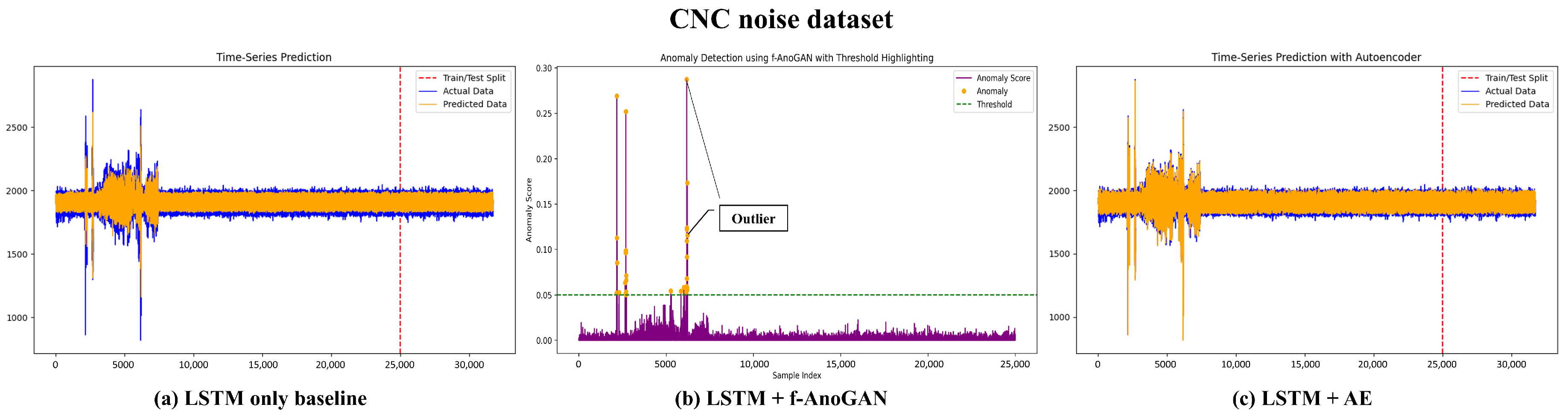
Result. The blue section in Figure 4 represents normal data generated from the operational noise of the machine in the CNC Noise Dataset. The purple curve in (b) represents the anomaly score for each sample, while the red dotted line indicates the threshold. Anomaly scores exceeding this threshold were considered anomalies. In (a,b), the orange dots represent anomalies that exceeded the threshold. In panel (a)∼(c), a significantly high anomaly score is observed within the 1000∼7000 sample range, indicating major anomalies detected in that segment. Beyond that range, the data appear relatively stable, with sporadic anomalies accurately identified. This pattern suggests that mechanical issues or noise were concentrated in specific intervals.

Figure 4.
This is the result of comparing time series prediction and anomaly detection performance using an LSTM-based model combined with other models. (a) Result of using the LSTM model alone. The difference between the orange (predicted data) and blue (actual data) represents the prediction error, highlighting the model’s limitation in clearly distinguishing anomaly data. (b) Result of combining LSTM with f-AnoGAN, visualizing the detection of anomaly data using an anomaly detection threshold. In each plot, the ability to clearly detect anomalies based on the anomaly score is demonstrated. (c) Result of combining LSTM with an Autoencoder (AE), where the time series data are predicted more accurately. By additionally using the AE, the model effectively detects anomaly data and improves prediction performance.
4.3. Question 2. LSTM-Based Latent ODE
LSTM is suitable for learning long-term dependencies in time series data and can effectively model the nonlinear and dynamic characteristics of CNC machine operation data. In this experiment, the input data consisted of sensor data (e.g., vibration noise) collected from CNC machines, while the output data included anomaly scores representing normal and abnormal machine states.
The latent ODE learned the latent representation of continuous time series data and predicted future states using an ODE (ordinary differential equation) solver. In latent space, the operational state of the CNC machine was represented by a low-dimensional latent vector, and the ODE solver modeled the change in this latent vector over time to predict future data.
In the combined model architecture, the LSTM encoder took sensor data as input, extracted time series features, and transformed them into latent space. The latent ODE module predicted future latent states based on the extracted latent vector, and the decoder transformed the predicted latent states back into the original data space to reconstruct the time series data and compute anomaly scores.
Experimental setup. StandardScaler performed normalization on the input features X with a mean of zero and a standard deviation of one. This eliminated differences in units or ranges among features and prevented specific features from having more influence during the training process. MinMaxScaler transformed the target variable Y to values between zero and one. The sequence length was set to 19, meaning the model used 19 past data points to make predictions. The gap between the past data and the future time step to predict was also set to 19, so the model took 10 past data points as input and predicted the value 10 steps ahead. Input data were generated using a sliding-window approach with the window_size length. To generate the predicted value, the gap was applied after the window_size to extract the prediction. The dataset was split into training and testing data, with 20% allocated for testing and the remaining 80% used for training.
Evaluation on CNC Dataset
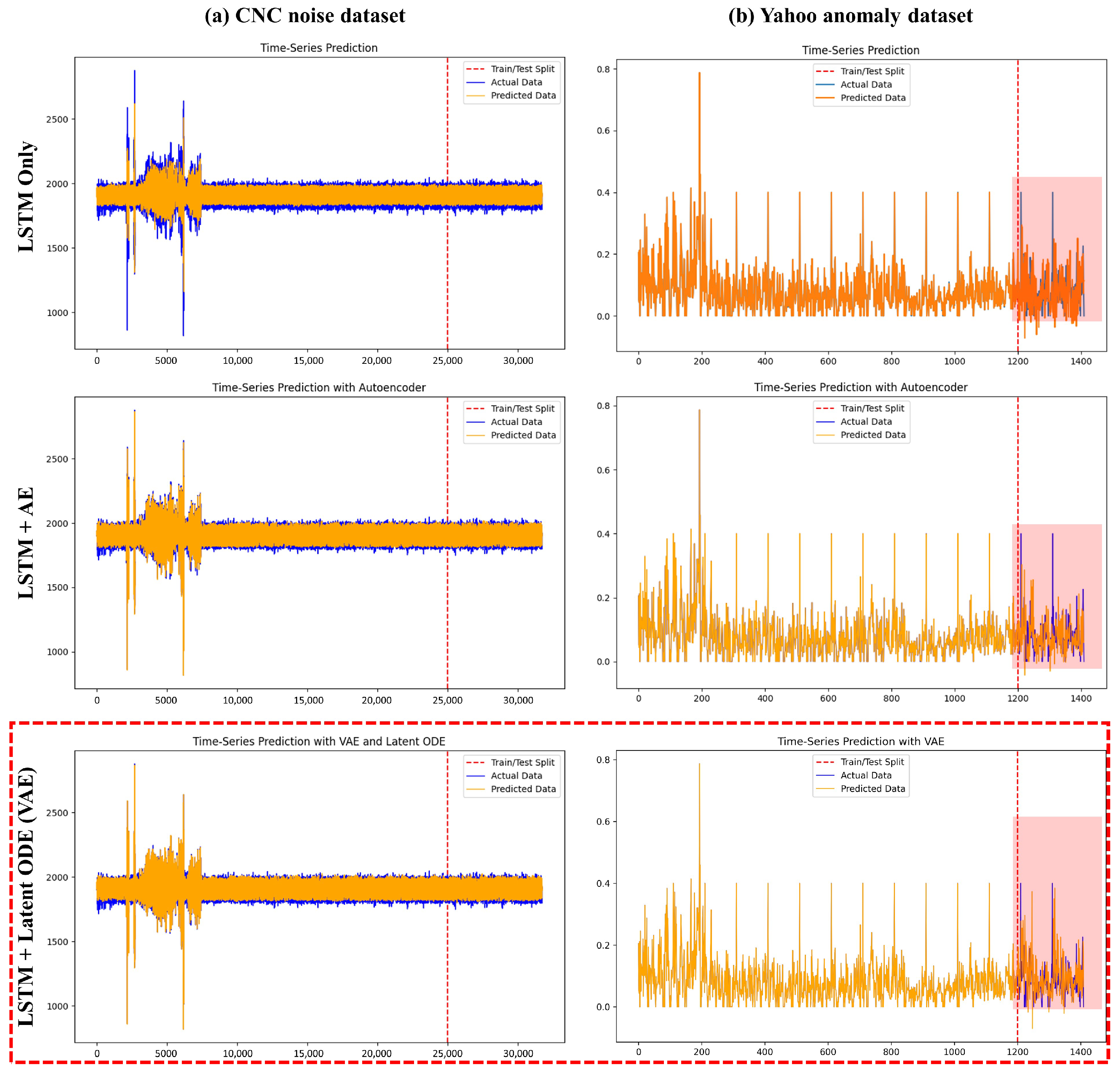
Result. In Figure 5a, the LSTM+latent ODE model, which was responsible for predictive maintenance based on noise data from manufacturing equipment (CNC Noise Dataset), was used to process time series data. The X-axis (time) represents the flow of time in the data, and the prediction model learned and evaluated the data along the time axis. The Y-axis (value) shows the normalized or scaled sound intensity of the recorded sound data from the equipment. The blue line (actual data) represents the actual sound data collected, which served as the reference data for model training and evaluation. The orange line (predicted data) shows the values predicted by the model, which were compared to the actual data to assess the model’s performance. The red vertical line (train/test split) indicates the point where the dataset was divided into training and testing sets. To the left of that line are the data the model learned from, while the right side comprises data that the model had not seen before.

Figure 5.
This study compares the performance of various LSTM-based model variants for time series data prediction on two datasets: (a) the CNC Noise Dataset and (b) the Yahoo Anomaly Dataset. The results highlight the differences in model performance across the datasets, with the LSTM+latent ODE (VAE) model consistently demonstrating the best performance on both datasets. In particular, the prediction detection capability shown in the red rectangular box of the Yahoo Anomaly Dataset demonstrated that this model could achieve highly advanced results when dealing with outliers and continuous complex patterns. The red vertical dotted line divided the entire dataset with an 8:2 ratio, with the left side used for training the model and the right side for validating the prediction model.
In the initial segment (training data), the predicted data (orange) closely matched the actual data (blue). Even in the test data segment, the model showed stable performance without significant deviation. There was a large amplitude fluctuation in the initial segment on the left side of the graph, which represents the portion where anomalies (noise) of the equipment were recorded, and this part was the focus of the prediction in this experiment. The stability of the results is shown in the testing segment (right side of the red dashed line), where the predicted values (orange) consistently follow a pattern similar to the actual values (blue), indicating that the model predicted noise effectively.
The goal of that experiment with the manufacturing equipment data was to enable the detection and prediction of anomalies based on the amount of noise in the fluctuating initial segment without additional filtering or preprocessing techniques, and the results showed that the model performed well in this regard. Additionally, optimizing the LSTM hyperparameters (such as the number of hidden nodes, number of layers) or the structure of the latent ODE further improved the model’s performance. These results demonstrate the utility of the model in predicting normal and abnormal states based on the noise generated by the manufacturing equipment.
4.4. Question 3. Verification of Model Generalization
Our experiment combined LSTM with the anomaly detection model (CBM) f-AnoGAN and the time series prediction model (PdM), and it seemed to proceed smoothly without any major issues. However, during the process of validating the model’s generalization performance using the Yahoo Anomaly Datasets [21], we had to change the model combination. The manufacturing equipment’s CNC Noise Dataset, as shown in the Figure 3 so far, had a simple structure. As shown in Figure 5a with LSTM+AE, the results were very good even without selecting a complex model algorithm. However, the detection of anomalies in Figure 5b did not perform well on the challenging Yahoo Anomaly Datasets. Therefore, to achieve satisfactory performance across all cases, we attempted to solve the problem by combining algorithms, as shown in the red dashed box (LSTM+latent ODE (VAE)) in Figure 5, and achieved improved results.
- f-AnoGAN Evaluation on Yahoo Dataset
Result. Figure 6a shows the Yahoo Anomaly Dataset, which is primarily designed for detecting anomalies in time series data and includes traffic, user activity, or web log data. Similar to panel (a), the purple curve shows the anomaly scores, while the green dashed line marks the threshold. Orange dots represent anomalies exceeding the threshold. In panel (b), a particularly high anomaly score is observed between the 200∼400 sample range, indicating major anomalies detected in this interval. Subsequent data are generally stable, with a few minor anomalies sporadically detected near the threshold. This suggests that abnormal data patterns occurred within specific time intervals.
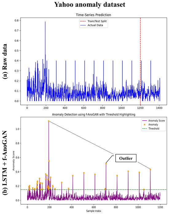
Figure 6.
(a) The Yahoo Anomaly Dataset is primarily designed for detecting anomalies in time series data. In (b), the purple curve represents the anomaly score, while the green dashed line indicates the threshold. The orange dots represent anomalies that exceed the threshold. In other words, as a condition-based maintenance approach, anomalies can be detected by setting a threshold to identify signs of failure before they occur. Therefore, all values exceeding the green dotted line indicate abnormal signs.
Both datasets demonstrated the effective anomaly detection capability of the f-AnoGAN and LSTM models. The threshold-based anomaly detection approach performed well in identifying outliers. In the CNC Noise Dataset, anomalies were primarily concentrated in specific segments, while the Yahoo Anomaly Dataset showed dispersed anomalies. These results reflect differences in the datasets’ characteristics and the underlying causes of anomalies. Moreover, they highlight the model’s adaptability to various datasets, showcasing its potential for flexible application.
- LSTM+Latent ODE Evaluation on Yahoo Dataset
Result. Figure 5b shows the results of using a high-dimensional time series dataset to objectively evaluate the proposed algorithm. As described above, the blue line (actual data) represents the actual observed data, which served as the reference for evaluating the model’s performance. The orange line (predicted data) represents the values predicted by the model. The vertical red dashed line (train/test split) indicates the division of the dataset into 80% training and 20% testing. The left side of the dashed line shows the data the model was trained on, while the right side shows the data predicted by the model. The red rectangle on the right represents the results predicted by our proposed LSTM+latent ODE (VAE) algorithm, and by comparing this with other models, we confirmed that our model achieved better accuracy.
In the training data section (before the red dashed line), the blue line (actual data) and the orange line (predicted data) align relatively well, indicating that the model effectively learned the normal patterns from the training data. In the test data section (after the red dashed line), the blue and orange lines also exhibit similar patterns, though minor discrepancies are observed in certain sections. In particular, in anomaly sections, where values increase or decrease rapidly, the orange line (predicted data) deviates slightly from the blue line (actual data). This suggests that the model may not have fully adapted to the anomaly sections or that additional data training is required.
The Yahoo Anomaly Dataset used in this study is characterized by frequent fluctuations and numerous anomalies, making anomaly detection challenging. These data characteristics may lead to prediction errors in certain sections. While there are limitations to address, the proposed combined algorithm demonstrated stable performance in complex time series data by leveraging LSTM’s time series learning capabilities, VAE’s latent space learning, and latent ODE’s continuous-time modeling. The model effectively learned and predicted normal data patterns in this research dataset, confirming its ability to handle general patterns reliably.
The performance of various LSTM-based models was analyzed using two datasets, (a) the CNC Noise Dataset and (b) the Yahoo Anomaly Dataset, to evaluate their ability to predict time series data. For the CNC Noise Dataset, which exhibits relatively clear patterns and a low outlier ratio, all models performed well during the training phase. The basic LSTM model achieved consistent predictions, although discrepancies emerged in the test phase, particularly in regions with high volatility. Incorporating an Autoencoder (LSTM+AE) improved prediction smoothness and reduced noise in the test data, though it still struggled with accurately handling outliers. In contrast, the advanced LSTM+latent ODE (VAE) model demonstrated superior performance by effectively capturing the dataset’s complex variability, maintaining high accuracy in both training and test phases, and outperforming other models.
The Yahoo Anomaly Dataset, characterized by high variability and frequent outliers, presented significant challenges for the basic LSTM model, which showed limited ability to capture anomalies in the test phase. The LSTM+AE model provided smoother predictions and performed better than the basic LSTM, but its performance remained inadequate for handling extreme outliers. On the other hand, the LSTM+latent ODE (VAE) model stood out due to its capability to learn continuous temporal representations, resulting in more accurate predictions of anomalies and complex patterns. This model effectively captured significant deviations, as highlighted in the red-shaded areas of the test phase results, surpassing the performance of all other models. Across both datasets, the LSTM+latent ODE (VAE) model emerged as the most effective, particularly excelling in scenarios with outliers and intricate patterns.
4.5. Limitations and Improvements
To evaluate the generalization performance of the combined algorithm, we conducted an additional analysis using the Yahoo Anomaly Dataset. This dataset, characterized by its small size and complex time-series data, posed significant challenges for accurate prediction. To address this, we combined multiple algorithms in stages. As a result, the LSTM+Latent ODE (VAE) model proposed in this paper successfully predicted patterns that other algorithms missed, as highlighted by the red square in Figure 5.
However, despite its superior performance compared to other models, the proposed model exhibited limitations in detecting anomalies in complex time series data like the Yahoo Anomaly Dataset. To address this, further techniques should be considered to enhance anomaly detection. Furthermore, future research could focus on increasing the quantity of training data or applying data augmentation to improve performance in sections containing anomalies.
In conclusion, the proposed model demonstrated its effectiveness in learning normal data patterns from the Yahoo Anomaly Dataset. However, further improvements in data and algorithms are required to improve prediction performance in complex sections such as anomalies.
Table 2 presents the results of the predictive model training using various methods in the CNC and Yahoo datasets. The performance of each method was evaluated using Mean Absolute Error (MAE) and Mean Squared Error (MSE), while anomaly detection performance was evaluated using the AUC (area under the curve) for some models.
Table 2.
This paper evaluated the performance of the proposed model and methodology using the CNC and Yahoo datasets. On the CNC dataset, the combination of LSTM+AE and LSTM+VAE achieved the lowest MAE and MSE scores. Similarly, on the Yahoo dataset, LSTM+AE demonstrated the best performance. The AUC scores of AnoGAN and f-AnoGAN were close to 0.5, indicating low classification performance. However, this did not pose an issue when visualizing anomaly detection and classification results. The proposed LSTM+latent ODE combined model maintained overall stable performance and was seamlessly integrated with the visualization, as shown in Figure 5b, to predict anomalies.
The LSTM-only model recorded relatively low MAE and MSE on both datasets, demonstrating its effectiveness in time series prediction. The LSTM+AE and LSTM+VAE models, which combined LSTM with an Autoencoder (AE) or a Variational Autoencoder (VAE), achieved even lower MAE and MSE than the LSTM-based model, indicating improved predictive performance.
Models utilizing a neural ordinary differential equation (ODE) showed high MAE and MSE on both datasets, suggesting that they were not suitable for these data types. Latent ODE models performed slightly worse than LSTM+AE and LSTM+VAE in terms of MAE and MSE but significantly outperformed neural ODE models.
The MAE is less sensitive to outliers and is intuitively interpretable, but it has scaling issues and can be distorted by noise. The MSE assigns greater weight to large errors, making it highly sensitive to outliers, but it can be misleading in noisy data and is less interpretable. The AUC provides stable performance evaluation even with class imbalance, but it lacks direct correlation with actual error rates and requires an additional threshold analysis. Therefore, rather than relying solely on numerical comparisons, the significance of our research findings is best understood through visualization in the red rectangular region of Figure 5b.
Overall, adding an AE or VAE to the LSTM network proved effective for improving predictive performance. Neural ODE models were not well suited to these datasets, while latent ODE models performed better than neural ODE models but slightly worse than LSTM+AE and LSTM+VAE models. However, in the red-shaded region of Figure 5b, the proposed LSTM+latent ODE (VAE) model showed the most accurate predictions. For anomaly detection models, the AUC values were close to 0.5, indicating a need for further performance improvement. However, no significant issues were observed when visualizing anomaly detection and classification results.
As a result, both datasets could be effectively predicted using LSTM-based models, highlighting the importance of dataset characteristics in model selection. Notably, the red-shaded region in Figure 5b serves as a key representation of the experimental results of this study.
5. Discussion
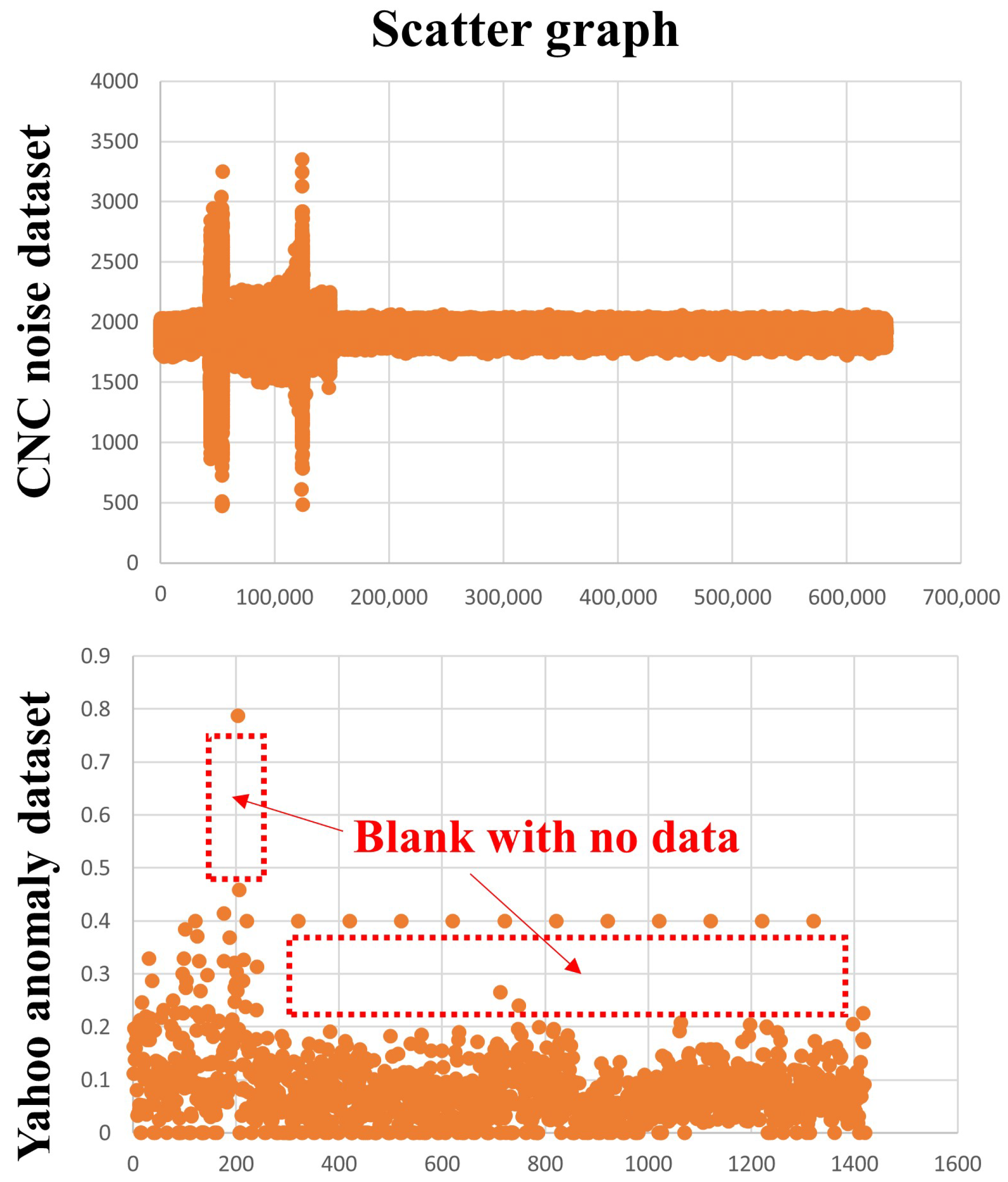
Figure 7 visualizes the issues by using a scatter graph instead of the conventional line graph. This scatter graph representation provides several insights. In the case of the CNC Noise Dataset, applying advanced algorithms allowed for the easy prediction of anomalies. However, when dealing with the volatility and anomalies of the Yahoo Anomaly Dataset, the basic LSTM model alone had limitations.

Figure 7.
The data distribution and specific anomalies are visually represented using a scatter plot. The CNC Noise Dataset exhibits a stable pattern in data density. In contrast, the Yahoo Anomaly Dataset contains large blank regions (approximately from 200 to 1400) where no data exist, resulting in a discontinuous data density.
To overcome these limitations, we focused on combining the advantages of state-of-the-art algorithms. Specifically, by integrating LSTM, VAE, f-AnoGAN, and latent ODEs, we achieved remarkable performance in handling highly volatile time series datasets. The reason why combining multiple algorithms led to better performance is evident in Figure 7. The Yahoo Anomaly Dataset contains a specific blank region (approximately from 200 to 1400), where no data exist. The presence of such data gaps makes it extremely challenging to detect precise anomalies. This suggests that certain points may be meaningless to the extent that it is difficult to distinguish between noise and anomalies.
In our research, we focused on predicting anomalies without preprocessing raw data. However, for future analyses involving datasets with such issues, an in-depth investigation of outliers and missing data in specific blank regions may be necessary. In such cases, post-processing techniques such as interpolation or missing-value handling should be considered to improve data reliability.
6. Conclusions
To ensure the stability and reliability of manufacturing equipment, we proposed two model combination approaches. The first one was an anomaly detection model (LSTM+f-AnoGAN) akin to condition-based maintenance (CBM), and the second one was a predictive maintenance (PdM) model (LSTM+latent ODE (VAE)). Both models demonstrated high performance, and the dual-algorithm approach was applied to enhance decision-making safety compared to using a single model. Specifically, the following two-step approach was utilized: (1) unsupervised learning and preprocessing without labels using f-AnoGAN to detect anomalies effectively. (2) predictive maintenance through combining a VAE and a latent ODE to analyze time series data and make predictions based on this analysis. The proposed models were evaluated through experiments using the Yahoo Anomaly Dataset, successfully detecting anomalies in manufacturing environments and demonstrating their general applicability. Through this theoretical and empirical analysis, we confirmed the proposed approach’s ability to enhance the stability and reliability of manufacturing equipment. By empirically detecting anomalies through sound and adjusting speed accordingly, we made progress in developing an algorithm and monitoring system to improve the performance of CNC machining equipment for roller-blade processing and to reasonably verify issues related to occurring errors.
Author Contributions
Conceptualization, J.C.; methodology, J.C.; software, J.C.; validation, J.C. and Z.X.; formal analysis, Z.X.; investigation, J.C.; resources, J.C. and Z.X.; data curation, J.C.; writing—original draft preparation, J.C.; writing—review and editing, K.K. and Z.X.; visualization, Z.X.; supervision, K.K.; project administration, J.C.; funding acquisition, K.K. All authors have read and agreed to the published version of the manuscript.
Funding
This research was supported by the Institute of Information & Communications Technology Planning & Evaluation (IITP), funded by the Korean government (Ministry of Science and ICT), under grant numbers RS-2022-00155885, IITP-2024-RS-2024-00423071, and IITP-2025-RS-2020-II201741, awarded for the Artificial Intelligence Convergence Innovation Human Resources Development Program at Hanyang University ERICA, the Global Research Support Program in the Digital Field, and the Innovative Human Resource Development for Local Intellectualization Program, respectively.
Data Availability Statement
Data are contained within the article.
Conflicts of Interest
The authors declare no conflicts of interest.
Abbreviations
The following abbreviations are used in this manuscript:
| CNC | Computerized numerical control |
| LSTM | Long short-term memory |
| RUL | Remaining useful life |
| ODE | Ordinary differential equation |
| CBM | Condition-based maintenance |
| PdM | Predictive maintenance |
References
- Calvanese, M.L.; Albertelli, P.; Matta, A.; Taisch, M. Analysis of energy consumption in CNC machining centers and determination of optimal cutting conditions. In Proceedings of the Re-Engineering Manufacturing for Sustainability: Proceedings of the 20th CIRP International Conference on Life Cycle Engineering, Singapore, 17–19 April 2013; Springer: Berlin/Heidelberg, Germany, 2013; pp. 227–232. [Google Scholar]
- Zhao, Y.; Zhou, J.; Dai, X.; Zhang, R.; Liu, Z.; Zhang, S.; Xu, Y. Efficient and sustainable short electric arc machining based on SKD-11 material. Alex. Eng. J. 2023, 64, 173–190. [Google Scholar]
- Dai, W.; Li, J.; Zhang, W.; Zheng, Z. Evaluation of fluences and surface characteristics in laser polishing SKD 11 tool steel. J. Mater. Process. Technol. 2019, 273, 116241. [Google Scholar]
- Prajapati, A.; Bechtel, J.; Ganesan, S. Condition based maintenance: A survey. J. Qual. Maint. Eng. 2012, 18, 384–400. [Google Scholar]
- Ahmad, R.; Kamaruddin, S. An overview of time-based and condition-based maintenance in industrial application. Comput. Ind. Eng. 2012, 63, 135–149. [Google Scholar]
- Hochreiter, S. Long Short-term Memory. Neural Comput. 1997, 9, 1735–1780. [Google Scholar] [CrossRef]
- Sherstinsky, A. Fundamentals of recurrent neural network (RNN) and long short-term memory (LSTM) network. Phys. D Nonlinear Phenom. 2020, 404, 132306. [Google Scholar] [CrossRef]
- Schlegl, T.; Seeböck, P.; Waldstein, S.M.; Schmidt-Erfurth, U.; Langs, G. Unsupervised anomaly detection with generative adversarial networks to guide marker discovery. In Proceedings of the International Conference on Information Processing in Medical Imaging, Boone, NC, USA, 25–30 June 2017; Springer: Berlin/Heidelberg, Germany, 2017; pp. 146–157. [Google Scholar]
- Xia, X.; Pan, X.; Li, N.; He, X.; Ma, L.; Zhang, X.; Ding, N. GAN-based anomaly detection: A review. Neurocomputing 2022, 493, 497–535. [Google Scholar]
- Sun, Y.; Yu, W.; Chen, Y.; Kadam, A. Time series anomaly detection based on GAN. In Proceedings of the 2019 Sixth International Conference on Social Networks Analysis, Management and Security (SNAMS), Granada, Spain, 22–25 October 2019; IEEE: Piscataway, NJ, USA, 2019; pp. 375–382. [Google Scholar]
- Coelho, C.; Costa, M.F.P.; Ferrás, L.L. Enhancing continuous time series modelling with a latent ODE-LSTM approach. Appl. Math. Comput. 2024, 475, 128727. [Google Scholar]
- Schlegl, T.; Seeböck, P.; Waldstein, S.M.; Langs, G.; Schmidt-Erfurth, U. f-AnoGAN: Fast unsupervised anomaly detection with generative adversarial networks. Med. Image Anal. 2019, 54, 30–44. [Google Scholar]
- Goodfellow, I.; Pouget-Abadie, J.; Mirza, M.; Xu, B.; Warde-Farley, D.; Ozair, S.; Courville, A.; Bengio, Y. Generative adversarial networks. Commun. ACM 2020, 63, 139–144. [Google Scholar]
- Chen, R.T.; Rubanova, Y.; Bettencourt, J.; Duvenaud, D.K. Neural ordinary differential equations. arXiv 2018, arXiv:1806.07366. [Google Scholar]
- Rubanova, Y.; Chen, R.T.; Duvenaud, D.K. Latent ordinary differential equations for irregularly-sampled time series. arXiv 2019, arXiv:1907.0390. [Google Scholar]
- Zhou, B.; Liu, S.; Hooi, B.; Cheng, X.; Ye, J. Beatgan: Anomalous rhythm detection using adversarially generated time series. In Proceedings of the International Joint Conference on Artificial Intelligence, Macao, China, 10–16 August 2019; Volume 2019, pp. 4433–4439. [Google Scholar]
- Si, X.S.; Wang, W.; Hu, C.H.; Zhou, D.H. Remaining useful life estimation—A review on the statistical data driven approaches. Eur. J. Oper. Res. 2011, 213, 1–14. [Google Scholar]
- Sikorska, J.Z.; Hodkiewicz, M.; Ma, L. Prognostic modelling options for remaining useful life estimation by industry. Mech. Syst. Signal Process. 2011, 25, 1803–1836. [Google Scholar]
- de Jonge, B.; Teunter, R.; Tinga, T. The influence of practical factors on the benefits of condition-based maintenance over time-based maintenance. Reliab. Eng. Syst. Saf. 2017, 158, 21–30. [Google Scholar]
- Wang, W. An overview of the recent advances in delay-time-based maintenance modelling. Reliab. Eng. Syst. Saf. 2012, 106, 165–178. [Google Scholar]
- Niu, Z.; Yu, K.; Wu, X. LSTM-based VAE-GAN for time-series anomaly detection. Sensors 2020, 20, 3738. [Google Scholar] [CrossRef]
- Lee, J.; Ni, J.; Singh, J.; Jiang, B.; Azamfar, M.; Feng, J. Intelligent maintenance systems and predictive manufacturing. J. Manuf. Sci. Eng. 2020, 142, 110805. [Google Scholar]
- Perera, J.C.; Gopalakrishnan, B.; Bisht, P.S.; Chaudhari, S.; Sundaramoorthy, S. A Sustainability-Based Expert System for Additive Manufacturing and CNC Machining. Sensors 2023, 23, 7770. [Google Scholar] [CrossRef]
- Achouch, M.; Dimitrova, M.; Ziane, K.; Sattarpanah Karganroudi, S.; Dhouib, R.; Ibrahim, H.; Adda, M. On predictive maintenance in industry 4.0: Overview, models, and challenges. Appl. Sci. 2022, 12, 8081. [Google Scholar] [CrossRef]
- Carvalho, T.P.; Soares, F.A.; Vita, R.; Francisco, R.d.P.; Basto, J.P.; Alcalá, S.G. A systematic literature review of machine learning methods applied to predictive maintenance. Comput. Ind. Eng. 2019, 137, 106024. [Google Scholar] [CrossRef]
- Zhang, W.; Yang, D.; Wang, H. Data-driven methods for predictive maintenance of industrial equipment: A survey. IEEE Syst. J. 2019, 13, 2213–2227. [Google Scholar] [CrossRef]
- He, W.; Zhang, L.; Hu, Y.; Zhou, Z.; Qiao, Y.; Yu, D. A Hybrid-Model-Based CNC Machining Trajectory Error Prediction and Compensation Method. Electronics 2024, 13, 1143. [Google Scholar] [CrossRef]
- Zhang, M.; Zhang, H.; Yan, W.; Jiang, Z.; Zhu, S. An integrated deep-learning-based approach for energy consumption prediction of machining systems. Sustainability 2023, 15, 5781. [Google Scholar] [CrossRef]
- Xie, S.; Xue, F.; Zhang, W.; Zhu, J. Data-Driven Predictive Maintenance Policy Based on Dynamic Probability Distribution Prediction of Remaining Useful Life. Machines 2023, 11, 923. [Google Scholar] [CrossRef]
- Gao, P.; Zhao, S.; Zheng, Y. Failure prediction of coal mine equipment braking system based on digital twin models. Processes 2024, 12, 837. [Google Scholar] [CrossRef]
- Teti, R.; Jemielniak, K.; O’Donnell, G.; Dornfeld, D. Advanced monitoring of machining operations. CIRP Ann. 2010, 59, 717–739. [Google Scholar] [CrossRef]
- Altintas, Y.; Ber, A. Manufacturing automation: Metal cutting mechanics, machine tool vibrations, and CNC design. Appl. Mech. Rev. 2001, 54, B84. [Google Scholar] [CrossRef]
- Schulz, H.; Moriwaki, T. High-speed machining. CIRP Ann. 1992, 41, 637–643. [Google Scholar] [CrossRef]
- Quintana, G.; Ciurana, J. Chatter in machining processes: A review. Int. J. Mach. Tools Manuf. 2011, 51, 363–376. [Google Scholar] [CrossRef]
- Vahdat, A.; Kautz, J. NVAE: A deep hierarchical variational autoencoder. Adv. Neural Inf. Process. Syst. 2020, 33, 19667–19679. [Google Scholar]
- Dai, B.; Wipf, D. Diagnosing and enhancing VAE models. arXiv 2019, arXiv:1903.05789. [Google Scholar]
- Choi, J.; Lee, S.; Kang, K. Espresso Crema Analysis with f-AnoGAN. Mathematics 2025, 13, 547. [Google Scholar] [CrossRef]
- Kingma, D.P.; Welling, M. Auto-encoding variational bayes. arXiv 2013, arXiv:1312.6114. [Google Scholar]
- Gondara, L. Medical image denoising using convolutional denoising autoencoders. In Proceedings of the 2016 IEEE 16th International Conference on Data Mining Workshops (ICDMW), Barcelona, Spain, 12–15 December 2016; IEEE: Piscataway, NJ, USA, 2016; pp. 241–246. [Google Scholar]
- Hashimoto, M.; Ide, Y.; Aritsugi, M. Anomaly detection for sensor data of semiconductor manufacturing equipment using a GAN. Procedia Comput. Sci. 2021, 192, 873–882. [Google Scholar]
- Abdul, M.S.; Sam, S.M.; Mohamed, N.; Hassan, N.H.; Azizan, A.; Yusof, Y.M. Peer to Peer Communication for the Internet of Things Using ESP32 Microcontroller for Indoor Environments. In Proceedings of the 2022 13th International Conference on Information and Communication Technology Convergence (ICTC), Jeju Island, Republic of Korea, 19–21 October 2022; IEEE: Piscataway, NJ, USA, 2022; pp. 1–6. [Google Scholar]
- Tang, D.; Wang, C.; Hu, Y.; Song, Y. Constitutive equation for hardened SKD11 steel at high temperature and high strain rate using the SHPB technique. In Proceedings of the Fourth International Conference on Experimental Mechanics, Singapore, 18–20 November 2009; SPIE: Bellingham, WA, USA, 2009; Volume 7522, pp. 1769–1780. [Google Scholar]


Disclaimer/Publisher’s Note: The statements, opinions and data contained in all publications are solely those of the individual author(s) and contributor(s) and not of MDPI and/or the editor(s). MDPI and/or the editor(s) disclaim responsibility for any injury to people or property resulting from any ideas, methods, instructions or products referred to in the content. |
© 2025 by the authors. Licensee MDPI, Basel, Switzerland. This article is an open access article distributed under the terms and conditions of the Creative Commons Attribution (CC BY) license (https://creativecommons.org/licenses/by/4.0/).