Mathematical Modeling of Economic Growth, Corruption, Employment and Inflation

Abstract

In this paper, we construct and propose a new mathematical model to study the dynamics of economic growth, corruption, unemployment, and inflation. The proposed model includes several relationships between these social and economic factors that have been studied and presented by economists. The mathematical model has several equilibrium points that are related to different socioeconomic scenarios. We perform a stability analysis of each of these equilibrium points in order to investigate the dynamics of the socioeconomic system. We find conditions for the local stability of the equilibrium points. We present numerical simulations to illustrate the theoretical results related to the stability of the equilibrium points. Moreover, we present numerical simulations in which periodic solutions arise due to Hopf bifurcations. The model allows us to better understand the impact that inflation, corruption, and unemployment have on the dynamics of economic growth. Finally, potential avenues for future research are presented.

1. Introduction

Many mathematical models have been developed for studying economics from different points of view [1,2,3,4,5,6]. For example, the stock market has been modeled using differential equations [7]. A very well-known model in economics is the Solow model and its variations [8,9,10,11]. Models based on partial differential equations have also been applied to socioeconomic aspects [12,13,14]. In addition, mathematical models based on structural equations and stochastic differential equations have also been applied to economic aspects [15]. Researchers have also developed mathematical models based on delay differential equations to study economics [16,17,18,19,20]. In [21], a spatial Solow model with a time delay was analyzed. In [22], the existence of a Hopf bifurcation in a one-sector optimal growth model with delay was studied. In addition, some works have applied control theory in conjunction with mathematical models to analyze potential economic policies [23,24,25,26,27]. Recently, mathematical models based on fractional differential equations have been applied to different economic aspects [28,29,30,31].

An important aspect that is sometimes found in economic mathematical models is bifurcation points and bifurcation boundaries [18,32,33,34]. An important bifurcation in economic models is the Hopf bifurcation. The importance of this bifurcation lies in the fact that limit cycles are relevant in the dynamics of the economy [35,36,37,38,39]. In particular, the appearance of Hopf bifurcations in several mathematical models that take into account inflation, corruption, and unemployment has been shown [40,41,42,43]. Oftentimes, Hopf bifurcations occur because of the presence of a time delay, which is due to the effect of previous states on the current states [44]. However, in many other economic models, a Hopf bifurcation arises from a change in the value of a parameter different from a time delay [45,46]. In [47], a mathematical model that includes corruption is analyzed, and conditions for backward bifurcations were found.

One way to evaluate the economic situation of a nation is by using the gross domestic product (GDP), which also allows measuring economic growth [48,49]. Economic growth rates are calculated from the difference of logs of the GDPs. In [50], a two-dimensional mathematical model was used to analyze and forecast GDP. In [51], a variety of stochastic ARIMA models were used to explore Nigeria’s GDP. The Solow model is a classical model that has been used extensively for modeling GDP using several factors such as capital, technology, and labor [9,13,52]. Inflation control is a crucial aspect that economic policymakers around the world try to enforce through several targeted policies. Inflation is the rate at which general levels of goods and services are rising, consequently leading to the falling of the purchasing power of a currency. Adequate socioeconomic research has been supported by policymakers, buttressing the fact that rapid and robustly sustainable economic growth can only occur with a well-controlled inflation rate. Inflation is a socioeconomic issue plaguing many nations, mainly because it has negative consequences for the operation of an economy and the welfare of its citizens. Economically, any nation with high inflation suffers a crippling effect on its economic growth, causing a direct increase in corruption levels while keeping unemployment at an all-time high. Economic growth is affected by inflation because high inflation rates cause higher interest rates and impact the price of goods [53]. The importance of studying and understanding the role that inflation plays and its complex and dynamic relationship with other socioeconomic phenomena cannot be overemphasized. This analysis is based on mathematical modeling real-life economic issues by approximating them with dynamical systems that reflect and capture the ever-changing nature of the problem. The inflation rate is measured primarily from the difference in the logs of CPI (consumer price index). In Africa, particularly Nigeria, the inflation rate skyrocketed from $13.25\%$ in 2020 to $31.7\%$ in the first quarter of 2024, with the highest inflation rate to date driven primarily by food inflation [54]. In Venezuela, at the end of 2017, the annual inflation rate was 2585% [55,56]. The main issues causing an increase in inflation in Nigeria are external debt, exchange rate, fiscal deficits, and money supply. It is no wonder that corruption and unemployment levels are high in Nigeria and other nations subjected to the same fate.

Corruption cripples the economic growth of a nation and hinders its full progress. It is an antisocial attitude that awards a variety of resources in an illegal way and affects society in various ways [57]. Clearly, there is no nation devoid of corruption as such; it can only be reduced or curbed minimally to lessen the adverse effect on economic growth, thus allowing a nation to reach its economic potential. Corruption is common in Nigeria. It has been estimated that Nigeria has lost more than 400 billion due to corruption during its history [58]. In [59], a causality relationship between corruption and inflation was investigated. Data from 180 countries over the period 1996–2014 were used. The authors found evidence that the inflation–corruption nexus is bidirectional. Moreover, the causal effect is more important from corruption to inflation. Also, it was found that corruption has an adverse effect on inflation. High inflation can lead to corruption by eroding the purchasing power of government officials and public servants. This can incentivize them to commit acts of corruption to maintain their standard of living. The existence of corruptive practices like tax evasions, budget deficits, increased public debt, etc. leads to higher inflation rates [59]. In [60], a significant positive association between corruption and inflation was found. Thus, in this article, we include these crucial socioeconomical bidirectional relationships between corruption and inflation in the proposed model. There are some mathematical models based on differential equations that have been proposed to study corruption [61,62,63,64,65].

According to economic theory, unemployment generally has a stable and inverse relationship with inflation, meaning that higher inflation is associated with a lower unemployment rate and vice versa. That is, when there are more employed people, they have the power to spend, leading to an increase in demand and, eventually, higher prices (inflation). The relationship between inflation and unemployment is not so black and white, as there are several factors that influence or affect this relationship. This relationship is often explained by the “Phillips Curve” that depicts this negative correlation between the two factors [66,67,68,69]. In [70], a similar result for the cyclical interaction between unemployment and inflation was obtained. Again, the more employed people are, the more they generally contribute to the economic growth of a nation. Thus, having a high unemployment rate poses a huge risk to any nation. It is in any nation’s best interest to reduce unemployment by creating avenues that provide more job opportunities for its citizens. With regard to economic growth in [71], it was found that economic growth and population have a positive relationship with long-term unemployment. In contrast, inflation was found to have a long-term negative relationship with unemployment. In the proposed model in this work, the relation between inflation and unemployment is presented indirectly through an intricate relationship with corruption and economic growth. The inflation increases corruption and corruption decreases economic growth. Then, lower economic growth increases unemployment.

There exists a complex relationship between inflation and economic growth, and there have been many points of view to reflect this. Some researchers argue that high inflation rates cause loss of purchasing power, higher interest rates, increased amounts of goods and services, etc., all of which have adverse effects on economic growth and tremendously slow it down. Thus, every economy attempts to always limit inflation while avoiding deflation to keep the economy running smoothly. This paper studies the dynamics of economic growth, corruption, unemployment, and inflation using a mathematical modeling approach. This approach aims at unraveling the intricate, interdependent dynamism that exists between these socioeconomic variables.

This article is structured as follows. In Section 2, we construct and develop the mathematical model. In Section 3, the stability analysis of the model is presented. Section 4 shows the numerical results that support the theoretical findings. Finally, Section 6 is devoted to conclusions.

2. The Proposed Mathematical Model

In this section, we propose a new mathematical model based on a previous model that considered and explored the relationship dynamics that exist between economic growth, corruption, and unemployment.

In [72], a mathematical model based on a nonlinear system of differential equations was proposed to study the relationship between economic growth ($G\left(t\right)$), corruption density ($C\left(t\right)$), and unemployment density ($U\left(t\right)$) was proposed. The model is given by

$$\begin{array}{cc}\hfill {\displaystyle \frac{dG\left(t\right)}{dt}}& =r_{1}G\left(t\right)\left(1-{\displaystyle \frac{G\left(t\right)}{K_1}}\right)-{\displaystyle \frac{\beta G\left(t\right)C\left(t\right)}{1+a\beta G\left(t\right)}},\hfill \\ \hfill {\displaystyle \frac{dC\left(t\right)}{dt}}& =\varphi {\displaystyle \frac{\beta G\left(t\right)C\left(t\right)}{1+a\beta G\left(t\right)}}-\mu C\left(t\right),\hfill \\ \hfill {\displaystyle \frac{dU\left(t\right)}{dt}}& =r_{2}U\left(t\right)\left(1-{\displaystyle \frac{U\left(t\right)+\xi G\left(t\right)}{K_2}}\right)-\kappa U\left(t\right),\hfill \end{array}$$

(1)

where $G\left(t\right)$ represents the economic growth of a nation, $C\left(t\right)$ denotes the corruption density, and $U\left(t\right)$ represents unemployment density. The parameters of this model (1) are $r_1$ is the intrinsic growth rate of the economy, $r_2$ is the rate of growth of unemployment, $K_1$ represents the economic carrying capacity, $K_2$ is the maximum potential size of unemployment, a represents the average time spent processing corruption, $\beta$ is the rate at which corrupt officials find economic assets, $\varphi$ is the specific conversion rate at which corrupt officials convert accessed resources into personal gains, $\mu$ is the rate at which corruption is reduced, $\xi$ is the rate at which economic growth generates new employment, and $\kappa$ represents new private business density $(\kappa <r_2)$. All of these parameters are assumed to be positive.

Upon the careful analysis of the mathematical model proposed in [72], it has been modified to include inflation. Inflation is a very crucial socioeconomic phenomenon that can significantly impact economic growth, corruption, and unemployment. These factors have an influence on investment decisions, business behavior, and overall social stability. Thus, it is vital to understand this interdependence for effective policy-making and economic planning.

When constructing the mathematical model, we take into account the fact that unemployment generally has a stable and inverse relationship with inflation. When there are more employed people, they have the power to spend, leading to an increase in demand and, eventually, higher prices (inflation). The model also takes into account that high inflation can lead to corruption by eroding the purchasing power of government officials and public servants. In addition, the existence of corruption leads to higher inflation rates [59]. Thus, we include the bidirectional relationships between corruption and inflation in the proposed model. In particular, the model uses a linear relationship for the variation of the corruption in terms of the inflation. In addition, for the variation of inflation, a positive linear relation is included. Besides these relationships, the model also includes others proposed in [72]. For instance, the variation of economic growth has a negative nonlinear relationship with corruption. Also, in the proposed model, the relation between inflation and unemployment is indirect through an intricate relationship with corruption and economic growth. The inflation increases corruption, and corruption decreases economic growth. Then, lower economic growth increases unemployment [59,60,72].

2.1. The Proposed Mathematical Model with Inflation

Let $I\left(t\right)$ represent the rate of inflation. Then, the proposed model becomes

$$\begin{array}{cc}\hfill {\displaystyle \frac{dG\left(t\right)}{dt}}& =r_{1}G\left(t\right)\left(1-{\displaystyle \frac{G\left(t\right)}{K_1}}\right)-{\displaystyle \frac{\beta G\left(t\right)C\left(t\right)}{1+a\beta G\left(t\right)}},\hfill \\ \hfill {\displaystyle \frac{dC\left(t\right)}{dt}}& =\varphi {\displaystyle \frac{\beta G\left(t\right)C\left(t\right)}{1+a\beta G\left(t\right)}}-\mu C\left(t\right)+pI\left(t\right),\hfill \\ \hfill {\displaystyle \frac{dU\left(t\right)}{dt}}& =r_{2}U\left(t\right)\left(1-{\displaystyle \frac{U\left(t\right)+\xi G\left(t\right)}{K_2}}\right)-\kappa U\left(t\right),\hfill \\ \hfill {\displaystyle \frac{dI\left(t\right)}{dt}}& =r_{4}C\left(t\right)-hI\left(t\right)U\left(t\right),\hfill \end{array}$$

(2)

where $r_4$ is the growth rate of inflation related to corruption, h represents factors that decrease inflation such as monetary and fiscal policies, etc., and p represents factors that increase inflation such as increased money supply, devaluation, rising wages, etc.

2.2. Positivity of the Model

Theorem 1. 

For system (2), $\dot{X}=f\left(X\right)$, the vector function f is non-negative for all $i=1,2,3,4$, $f_i\left(X\right)\ge 0$, where $X\in {\mathbb{R}}^4\ge 0$ such that $X_i=0$ denotes the i-th element of X and $X=\left[\begin{array}{c}G\\ C\\ U\\ I\end{array}\right]$.

Proof. 

For $G,C,U,I\ge 0$, $i=1,2,3,4$, and for all parameters positive,

$$\begin{array}{cc}\hfill f_1(0,C,U,I)& =0,\hfill \\ \hfill f_2(G,0,U,I)& =pI>0,\hfill \\ \hfill f_3(G,C,0,I)& =0,\hfill \\ \hfill f_4(G,C,U,0)& =r_{4}C>0.\hfill \end{array}$$

□

This proves the positivity of the solutions of system (2), which is a realistic representation of real-world scenarios whereby state variables can only assume non-negative values. Thus, with positive initial conditions, the system will always generate positive values for the state variables regardless of how the system evolves over time. This positivity aspect is crucial in any mathematical model related to economic positive quantities in order to obtain realistic outcomes from the model [17,73,74,75]. It is important to point out that, sometimes, the numerical method used to solve a system of differential equations can generate spurious and negative solutions despite the positivity of the solutions having been proved. Thus, a reliable numerical method that generates non-negative solutions is necessary (see [76,77,78]).

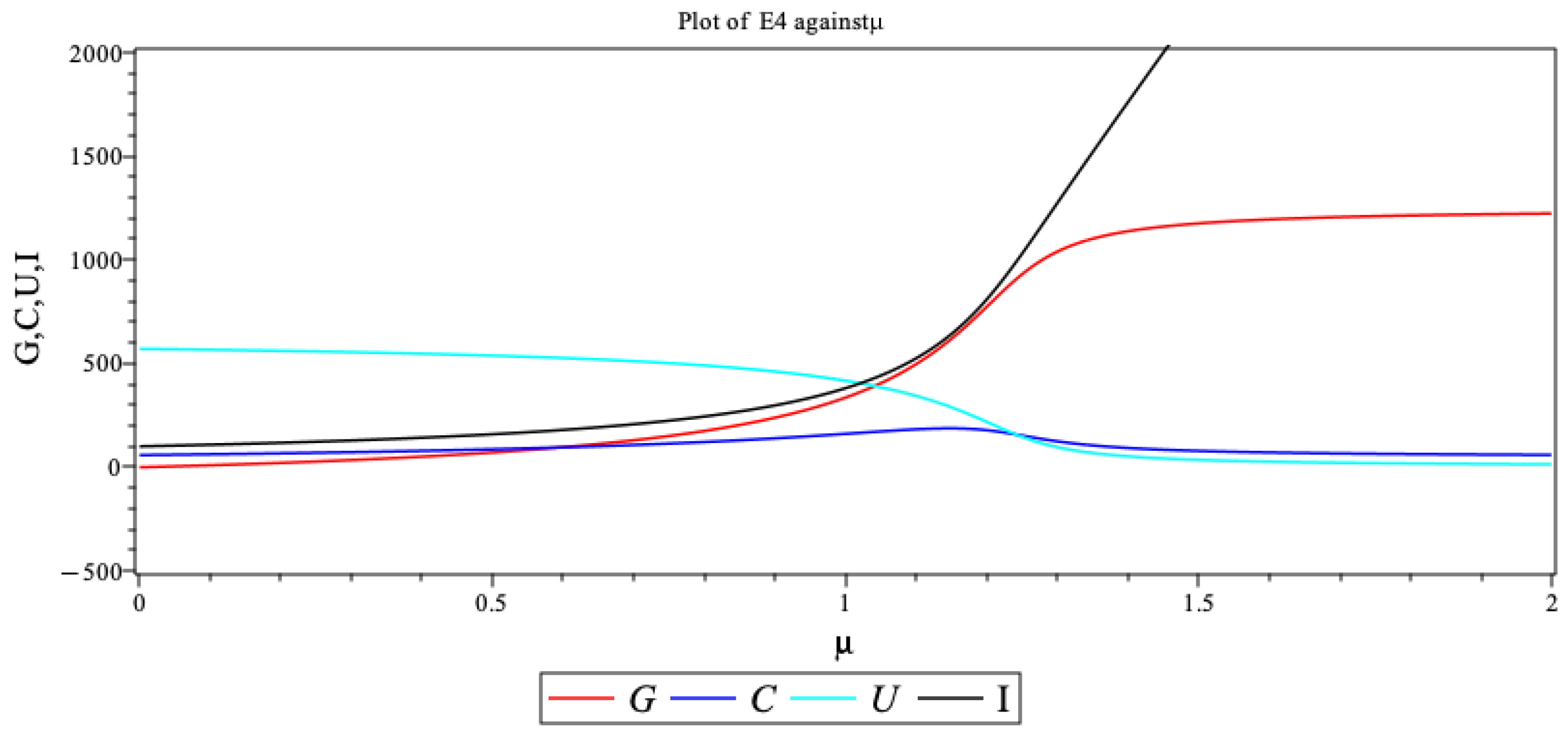
3. Stability Analysis of the Model

Here, the mathematical model (2) is qualitatively analyzed to investigate the stability of its steady states. First, we determine the equilibrium points of the system and perform a local stability analysis for each of them. We also search for conditions such that Hopf bifurcations arise.

From the theory of ordinary differential equations, it can be proved that, for any initial condition $\left(G\right(0),C(0),U(0),I(0\left)\right)$, there exists a unique solution $\left(G\right(t),C(t),U(t),I(t\left)\right)$ that satisfies system (2) [79,80].

3.1. Equilibrium Points

To initiate the stability analysis, we first find the equilibrium points of the mathematical model (2), which are states in which the system remains unchanged. This is done by equating the right-hand side of system (2) to zero and solving the system.

$$\begin{array}{cc}\hfill 0& =r_{1}G\left(1-{\displaystyle \frac{G}{K_1}}\right)-{\displaystyle \frac{\beta GC}{1+a\beta G}},\hfill \\ \hfill 0& =\varphi {\displaystyle \frac{\beta GC}{1+a\beta G}}-\mu C+pI,\hfill \\ \hfill 0& =r_{2}U(1-{\displaystyle \frac{U+\xi G}{K_2}})-\kappa U,\hfill \\ \hfill 0& =r_{4}C-IUh.\hfill \end{array}$$

(3)

Solving these equations, one ascertains that the equilibrium points are as follows:

• The Trivial equilibrium point $E_0=\{G=0,C=0,U=0,I=0\}$ represents the complete absence of economic resources, corruption, unemployment, and inflation.
• The axial equilibrium point $E_1=\left\{G=0,C=0,U={\displaystyle \frac{{\mathit{K}}_{\mathit{2}}\left({\mathit{r}}_{\mathit{2}}-\kappa \right)}{{\mathit{r}}_{\mathit{2}}}},I=0\right\}$ represents a state with no economic growth, no corruption, and no inflation with some unemployment level.
• The Axial equilibrium point $E_2=\{G={\mathit{K}}_{\mathit{1}},C=0,U=0,I=0\}$ depicts a state with maximum economic growth but without corruption, unemployment or inflation.
• The equilibrium point $E_3=\left\{G={\mathit{K}}_{\mathit{1}},C=0,U={\displaystyle \frac{{\mathit{K}}_{\mathit{2}}{\mathit{r}}_{\mathit{2}}-{\mathit{K}}_{\mathit{1}}{\mathit{r}}_{\mathit{2}}\xi -\kappa \mathit{K}\mathit{2}}{{\mathit{r}}_{\mathit{2}}}},I=0\right\}$ represents a state with maximum economic growth, no corruption, no inflation, and a specific unemployment level determined by job creation density and resource depletion rates.
• The interior equilibrium point $E_4=(G^{\ast },C^{\ast },U^{\ast },I^{\ast })$ with
  • $G^{\ast }={\displaystyle \frac{\sqrt{B}+Y\beta -h\mu r_2\xi }{X}}$,
  • $C^{\ast }=-{\displaystyle \frac{r_1(\sqrt{B}+Y\beta -h\mu r_2\xi -K_{1}X)(a\beta \sqrt{B}+aY{\beta }^2-a\beta h\mu r_2\xi +X)}{X^2{K}_1\beta }}$,
  • $U^{\ast }={\displaystyle \frac{h\mu r_2\xi -M\beta K_{2}Nh+a\beta p{r}_2{r}_4-\sqrt{B}}{2h\beta r_{2}M}}$,
  • $I^{\ast }=-{\displaystyle \frac{r_1(\sqrt{B}+Y\beta -h\mu r_2\xi -K_{1}X)(\beta M\sqrt{B}+MY{\beta }^2-h\mu r_2\xi M\beta +\mu X)}{X^{2}p\beta K_1}}$.
• The interior equilibrium point $E_5=(G^{\ast },C^{\ast },U^{\ast },I^{\ast })$ with
  • $G^{\ast }={\displaystyle \frac{-\sqrt{B}+Y\beta -h\mu r_2\xi }{X}}$,
  • $C^{\ast }=-{\displaystyle \frac{r_1(-\sqrt{B}+Y\beta -h\mu r_2\xi -K_{1}X)(-a\beta \sqrt{B}+aY{\beta }^2-a\beta h\mu r_2\xi +X)}{X^2{K}_1\beta }}$,
  • $U^{\ast }={\displaystyle \frac{h\mu r_2\xi -M\beta K_{2}Nh+a\beta p{r}_2{r}_4+\sqrt{B}}{2h\beta r_{2}M}}$,
  • $I^{\ast }=-{\displaystyle \frac{r_1(-\sqrt{B}+Y\beta -h\mu r_2\xi -K_{1}X)(-\beta M\sqrt{B}+MY{\beta }^2-h\mu r_2\xi M\beta +\mu X)}{X^{2}p\beta K_1}}$,

where

• $M=a\mu -\varphi$
• $N=\kappa -r_2$
• $Q=M^2{N}^2{\beta }^2{h}^2{K}_2^2$
• $R=a^2{\beta }^2{p}^2{r}_2^2{r}_4^2$
• $S=h^2{\mu }^2{r}_2^2{\xi }^2$
• $T=-a\beta p{r}_4+h\mu \xi$
• $W=-{\displaystyle \frac{a\mu }{2}}+M$
• $V=2r_2-2\kappa +N$
• $X=2M\beta h{r}_2\xi$
• $Y=\left(M{K}_{2}Vh-p{r}_2{r}_{4}a\right)$
• $B=-2r_{2}h(2Wp{r}_2{r}_4\xi +MNT{K}_2)\beta +Q+R+S$.

3.2. Stability Analysis of Equilibrium Points

We study the local stability of each equilibrium point by the linearization of system (2). Let $X=(G,C,U,I)$ be the state vector. Then, the Jacobian of system (2) is

$$\begin{array}{c}\hfill J\left(X\right)=\left(\begin{array}{cccc}{\mathit{r}}_{\mathit{1}}\left(1-{\displaystyle \frac{2G}{{\mathit{K}}_{\mathit{1}}}}\right)-{\displaystyle \frac{\beta C}{{(a\beta G+1)}^2}}& -{\displaystyle \frac{\beta G}{a\beta G+1}}& 0& 0\\ \\ {\displaystyle \frac{\varphi \beta C}{{(a\beta G+1)}^2}}& {\displaystyle \frac{\varphi \beta G}{a\beta G+1}}-\mu & 0& p\\ \\ -{\displaystyle \frac{{\mathit{r}}_{\mathit{2}}U\xi }{{\mathit{K}}_{\mathit{2}}}}& 0& {\mathit{r}}_{\mathit{2}}\left(1-{\displaystyle \frac{G\xi +U}{{\mathit{K}}_{\mathit{2}}}}\right)-{\displaystyle \frac{{\mathit{r}}_{\mathit{2}}U}{{\mathit{K}}_{\mathit{2}}}}-\kappa & 0\\ \\ 0& {\mathit{r}}_{\mathit{4}}& -Ih& -Uh\end{array}\right).\end{array}$$

(4)

3.2.1. Stability Analysis of $E_0$

Theorem 2. 

The trivial equilibrium point $E_0=(0,0,0,0)$ is always unstable.

Proof. 

The Jacobian from (4) evaluated at $E_0$ is

$$\begin{array}{c}\hfill J\left(E_0\right)=\left[\begin{array}{cccc}{\mathit{r}}_{\mathit{1}}& 0& 0& 0\\ 0& -\mu & 0& p\\ 0& 0& {\mathit{r}}_{\mathit{2}}-\kappa & 0\\ 0& {\mathit{r}}_{\mathit{4}}& 0& 0\end{array}\right].\end{array}$$

(5)

The eigenvalues of the matrix given in (5) are

$$\begin{array}{c}\hfill \lambda =\left[\begin{array}{c}{\mathit{r}}_{\mathit{1}}\\ \\ -{\displaystyle \frac{\mu }{2}}+{\displaystyle \frac{\sqrt{{\mu }^2+4p{\mathit{r}}_{\mathit{4}}}}{2}}\\ \\ -{\displaystyle \frac{\mu }{2}}-{\displaystyle \frac{\sqrt{{\mu }^2+4p{\mathit{r}}_{\mathit{4}}}}{2}}\\ \\ {\mathit{r}}_{\mathit{2}}-\kappa \end{array}\right].\end{array}$$

(6)

By the principle of eigenvalue analysis, local stability is guaranteed if the real part of all the eigenvalues is negative. But, ${\lambda }_1=r_1$ is always positive since $r_1$ is positive. Therefore, $E_0$ is always unstable. □

All the eigenvalues are strictly real eigenvalues. Thus, they cannot become complex regardless of the values of the parameters, and Hopf bifurcation cannot arise from $E_0$.

3.2.2. Stability Analysis of $E_1$

Theorem 3. 

The axial equilibrium point $E_1=\left(0,0,{\displaystyle \frac{{\mathit{K}}_{\mathit{2}}\left({\mathit{r}}_{\mathit{2}}-\kappa \right)}{{\mathit{r}}_{\mathit{2}}}},0\right)$ is always unstable.

Proof. 

The Jacobian matrix (4) evaluated at $E_1$ is

$$\begin{array}{c}\hfill J\left(E_1\right)=\left[\begin{array}{cccc}{\mathit{r}}_{\mathit{1}}& 0& 0& 0\\ 0& -\mu & 0& p\\ \left(\kappa -{\mathit{r}}_{\mathit{2}}\right)\xi & 0& {\mathit{r}}_{\mathit{2}}\left(1+{\displaystyle \frac{\kappa -{\mathit{r}}_{\mathit{2}}}{{\mathit{r}}_{\mathit{2}}}}\right)-{\mathit{r}}_{\mathit{2}}& 0\\ 0& {\mathit{r}}_{\mathit{4}}& 0& {\displaystyle \frac{{\mathit{K}}_{\mathit{2}}\left(\kappa -{\mathit{r}}_{\mathit{2}}\right)h}{{\mathit{r}}_{\mathit{2}}}}\end{array}\right].\end{array}$$

(7)

The eigenvalues of the matrix given in (7) are,

$$\begin{array}{c}\hfill \lambda =\left[\begin{array}{c}{\mathit{r}}_{\mathit{1}}\\ \\ \kappa -{\mathit{r}}_{\mathit{2}}\\ \\ {\displaystyle \frac{{\mathit{K}}_{\mathit{2}}h\kappa -{\mathit{K}}_{\mathit{2}}h{\mathit{r}}_{\mathit{2}}-{\mathit{r}}_{\mathit{2}}\mu +\sqrt{B}}{2{\mathit{r}}_{\mathit{2}}}}\\ \\ {\displaystyle \frac{{\mathit{K}}_{\mathit{2}}h\kappa -{\mathit{K}}_{\mathit{2}}h{\mathit{r}}_{\mathit{2}}-{\mathit{r}}_{\mathit{2}}\mu -\sqrt{B}}{2{\mathit{r}}_{\mathit{2}}}}\end{array}\right],\end{array}$$

(8)

where $B={\mathit{K}}_{\mathit{2}}^2{h}^2{\kappa }^2-2{\mathit{K}}_{\mathit{2}}^2{h}^2\kappa {\mathit{r}}_{\mathit{2}}+{\mathit{K}}_{\mathit{2}}^2{h}^2{\mathit{r}}_{\mathit{2}}^2+2{\mathit{K}}_{\mathit{2}}h\kappa \mu {\mathit{r}}_{\mathit{2}}-2{\mathit{K}}_{\mathit{2}}h\mu {\mathit{r}}_{\mathit{2}}^2+{\mu }^2{\mathit{r}}_{\mathit{2}}^2+4p{\mathit{r}}_{\mathit{4}}{\mathit{r}}_{\mathit{2}}^2$. However, B can be rearranged as

$$\begin{array}{cc}\hfill B& ={\mathit{K}}_{\mathit{2}}^2{h}^2{\kappa }^2-2{\mathit{K}}_{\mathit{2}}^2{h}^2\kappa {\mathit{r}}_{\mathit{2}}+{\mathit{K}}_{\mathit{2}}^2{h}^2{\mathit{r}}_{\mathit{2}}^2+2{\mathit{K}}_{\mathit{2}}h\kappa \mu {\mathit{r}}_{\mathit{2}}-2{\mathit{K}}_{\mathit{2}}h\mu {\mathit{r}}_{\mathit{2}}^2+{\mu }^2{\mathit{r}}_{\mathit{2}}^2+4p{\mathit{r}}_{\mathit{4}}{\mathit{r}}_{\mathit{2}}^2\hfill \\ \hfill & =(\kappa -r_2)\left(K_2^2{h}^2(\kappa -r_2)+2K_{2}h\mu r_2\right)+{\mu }^2{\mathit{r}}_{\mathit{2}}^2+4p{\mathit{r}}_{\mathit{4}}{\mathit{r}}_{\mathit{2}}^2\hfill \\ \hfill & ={(\kappa -r_2)}^2+{\displaystyle \frac{2\mu r_2}{K_{2}h}}(\kappa -r_2)+{\displaystyle \frac{{\mu }^2{\mathit{r}}_{\mathit{2}}^2+4p{\mathit{r}}_{\mathit{4}}{\mathit{r}}_{\mathit{2}}^2}{K_2^2{h}^2}}.\hfill \end{array}$$

Completing the square in terms of $(\kappa -r_2)$ gives

$$\begin{array}{c}\hfill B={\left((\kappa -r_2)+{\displaystyle \frac{\mu r_2}{K_{2}h}}\right)}^2+{\displaystyle \frac{4p{r}_4{r}_2^2}{K_2^2{h}^2}}>0.\end{array}$$

Then, the eigenvalues ${\lambda }_3$ and ${\lambda }_4$ are strictly real eigenvalues. Again, the local stability is guaranteed if the real part of all eigenvalues is negative. But, ${\lambda }_1=r_1$ is always positive. Thus, $E_1$ is unstable. □

All the eigenvalues are strictly real eigenvalues, Thus, they cannot become complex regardless of the values of the parameters, and Hopf bifurcation cannot arise from $E_1$.

3.2.3. Stability Analysis of $E_2$

Theorem 4. 

The Axial equilibrium point $E_2=({\mathit{K}}_{\mathit{1}},0,0,0)$ is always unstable.

Proof.  

The Jacobian matrix from (4) evaluated at $E_2$ is

$$\begin{array}{c}\hfill J\left(E_2\right)=\left[\begin{array}{cccc}-{\mathit{r}}_{\mathit{1}}& -{\displaystyle \frac{\beta {\mathit{K}}_{\mathit{1}}}{{\mathit{K}}_{\mathit{1}}a\beta +1}}& 0& 0\\ \\ 0& {\displaystyle \frac{\varphi \beta {\mathit{K}}_{\mathit{1}}}{{\mathit{K}}_{\mathit{1}}a\beta +1}}-\mu & 0& p\\ \\ 0& 0& {\mathit{r}}_{\mathit{2}}\left(1-{\displaystyle \frac{{\mathit{K}}_{\mathit{1}}\xi }{{\mathit{K}}_{\mathit{2}}}}\right)-\kappa & 0\\ \\ 0& {\mathit{r}}_{\mathit{4}}& 0& 0\end{array}\right].\end{array}$$

(9)

The eigenvalues of the matrix given in (9) are

$$\begin{array}{c}\hfill \left[\begin{array}{c}{\lambda }_1\\ \\ {\lambda }_2\\ \\ {\lambda }_3\\ \\ {\lambda }_4\end{array}\right]=\left[\begin{array}{c}-{\mathit{r}}_{\mathit{1}}\\ \\ {\displaystyle \frac{-(a\mu -\varphi )K_1\beta +\sqrt{D}-\mu }{2(K_{1}a\beta +1)}}\\ \\ {\displaystyle \frac{-(a\mu -\varphi )K_1\beta -\sqrt{D}-\mu }{2(K_{1}a\beta +1)}}\\ \\ -{\displaystyle \frac{{\mathit{K}}_{\mathit{1}}{\mathit{r}}_{\mathit{2}}\xi +\left(\kappa -{\mathit{r}}_{\mathit{2}}\right){\mathit{K}}_{\mathit{2}}}{{\mathit{K}}_{\mathit{2}}}}\end{array}\right].\end{array}$$

(10)

The conditions for local stability of $E_2$ are

• ${\lambda }_1=-r_1<0$. This is always certain since $r_1>0$.
• ${\displaystyle \frac{K_1{r}_2\xi +(\kappa -r_2)K_2}{K_2}}>0$. Thus, this guarantees that ${\lambda }_4<0$.
• $\Re ({\lambda }_2,{\lambda }_3)<0$. If $D<0$ then one obtain that $\Re ({\lambda }_2,{\lambda }_3)={\displaystyle \frac{-(a\mu -\varphi )K_1\beta -\mu }{2(K_{1}a\beta +1)}}$. If $D\ge 0$ then $\Re ({\lambda }_2,{\lambda }_3)={\displaystyle \frac{-(a\mu -\varphi )K_1\beta -\sqrt{D}-\mu }{2(K_{1}a\beta +1)}}$.

The discriminant D that appears in Equation (10) is given as

$$\begin{array}{cc}\hfill D& ={\left(K_{1}a\beta \mu \right)}^2+{\left(K_1\beta \varphi \right)}^2+2K_{1}a\beta {\mu }^2-2K_1^2{\beta }^{2}a\mu \varphi -2K_1\beta \mu \varphi +4{\left(K_{1}a\beta \right)}^{2}p{r}_4+8K_{1}a\beta p{r}_4+{\mu }^2+4p{r}_4\hfill \\ \hfill & =2K_1\beta \mu (a\mu -\varphi )+K_1^2{\beta }^{2}a\mu (a\mu -\varphi )-K_1^2{\beta }^2\varphi (a\mu -\varphi )+4p{r}_4({\left(K_{1}a\beta \right)}^2+2\left(K_{1}a\beta \right)+1)+{\mu }^2\hfill \\ \hfill & =(a\mu -\varphi )\left(K_1^2{\beta }^2(a\mu -\varphi )+2K_1\beta \mu \right)+4p{r}_4({\left(K_{1}a\beta \right)}^2+2\left(K_{1}a\beta \right)+1)+{\mu }^2\hfill \\ \hfill & ={\left((a\mu -\varphi )K_1\beta \right)}^2+2\mu \left((a\mu -\varphi )K_1\beta \right)+4p{r}_4\left({\left(K_{1}a\beta \right)}^2+2\left(K_{1}a\beta \right)+1\right)+{\mu }^2\hfill \\ \hfill & ={\left(\left((a\mu -\varphi )K_1\beta \right)+\mu \right)}^2+4p{r}_4\left({\left(K_{1}a\beta \right)}^2+2\left(K_{1}a\beta \right)+1\right)\hfill \\ \hfill & ={\left(\left((a\mu -\varphi )K_1\beta \right)+\mu \right)}^2+4p{r}_4{\left(K_{1}a\beta +1\right)}^2\ge 0,\hfill \end{array}$$

where D is rewritten as a quadratic expression in terms of $((a\mu -\varphi )K_1\beta +\mu )$ and $(K_{1}a\beta +1)$. Clearly, the discriminant D is always non-negative. Thus, the eigenvalues ${\lambda }_2$ and ${\lambda }_3$ are always real.

Substituting the expression of D in Equation (10) for ${\lambda }_2$ and ${\lambda }_3$ gives

$$\begin{array}{cc}\hfill {\lambda }_2,{\lambda }_3& ={\displaystyle \frac{-\left((a\mu -\varphi )K_1\beta +\mu \right)\pm \sqrt{{\left((a\mu -\varphi )K_1\beta +\mu \right)}^2+4p{r}_4{\left(K_{1}a\beta +1\right)}^2}}{2(K_{1}a\beta +1)}}.\hfill \end{array}$$

Now, let us analyze the signs of the eigenvalues ${\lambda }_2$ and ${\lambda }_3$.

case 1: If $(a\mu -\varphi )K_1\beta +\mu >0$, then ${\lambda }_2>0$ and ${\lambda }_3<0$.

case 2: If $(a\mu -\varphi )K_1\beta +\mu <0$, then ${\lambda }_2>0$ and ${\lambda }_3<0$.

In both cases, ${\lambda }_2>0$. Thus, the equilibrium point $E_2$ is always unstable since the Jacobian matrix evaluated at $E_2$ always has at least a positive eigenvalue. □

Now, since all the eigenvalues of the Jacobian matrix (4) evaluated at $E_2$ are real, then Hopf bifurcations cannot arise from $E_2$.

3.2.4. Stability Analysis of $E_3$

Theorem 5. 

The equilibrium point $E_3=\left({\mathit{K}}_{\mathit{1}},0,{\displaystyle \frac{{\mathit{K}}_{\mathit{2}}{\mathit{r}}_{\mathit{2}}-{\mathit{K}}_{\mathit{1}}{\mathit{r}}_{\mathit{2}}\xi -\kappa {\mathit{K}}_{\mathit{2}}}{{\mathit{r}}_{\mathit{2}}}},0\right)$ is locally asymptotically stable if ${\displaystyle \frac{K_1{r}_2\xi +(\kappa -r_2)K_2}{K_2}}<0$, $c_1>0$ and $c_0>0$.

Proof. 

The Jacobian matrix (4) evaluated at $E_3$ is

$$\begin{array}{c}\hfill J\left(E_3\right)=\left[\begin{array}{cccc}-{\mathit{r}}_{\mathit{1}}& -{\displaystyle \frac{\beta {\mathit{K}}_{\mathit{1}}}{{\mathit{K}}_{\mathit{1}}a\beta +1}}& 0& 0\\ 0& {\displaystyle \frac{\varphi \beta {\mathit{K}}_{\mathit{1}}}{{\mathit{K}}_{\mathit{1}}a\beta +1}}-\mu & 0& p\\ {\displaystyle \frac{\left({\mathit{K}}_{\mathit{2}}\left(\kappa -{\mathit{r}}_{\mathit{2}}\right)+{\mathit{K}}_{\mathit{1}}{\mathit{r}}_{\mathit{2}}\xi \right)\xi }{{\mathit{K}}_{\mathit{2}}}}& 0& {\displaystyle \frac{{\mathit{K}}_{\mathit{2}}\left(\kappa -{\mathit{r}}_{\mathit{2}}\right)+{\mathit{K}}_{\mathit{1}}{\mathit{r}}_{\mathit{2}}\xi }{{\mathit{K}}_{\mathit{2}}}}& 0\\ 0& {\mathit{r}}_{\mathit{4}}& 0& {\displaystyle \frac{\left(\left({\mathit{K}}_{\mathit{1}}\xi -{\mathit{K}}_{\mathit{2}}\right){\mathit{r}}_{\mathit{2}}+\kappa {\mathit{K}}_{\mathit{2}}\right)h}{{\mathit{r}}_{\mathit{2}}}}\end{array}\right].\end{array}$$

(11)

Computing the eigenvalues one obtains the following,

$$\begin{array}{cc}\hfill {\lambda }_1& =-r_1<0,\hfill \\ \hfill {\lambda }_2& ={\displaystyle \frac{K_1{r}_2\xi +(\kappa -r_2)K_2}{K_2}}<0,\mathrm{if}{K}_2>{\displaystyle \frac{K_1{r}_2\xi }{r_2-\kappa }},\hfill \\ \hfill {\lambda }_3& ={\displaystyle \frac{(a{K}_1^{2}h\xi \beta +((-ah{K}_2-a\mu +\varphi )\beta +h\xi )K_1-h{K}_2-\mu )r_2+a\beta h\kappa K_1{K}_2+h\kappa K_2-\sqrt{D}}{2r_2(a\beta K_1+1)}},\hfill \\ \hfill {\lambda }_4& ={\displaystyle \frac{(a{K}_1^{2}h\xi \beta +((-ah{K}_2-a\mu +\varphi )\beta +h\xi )K_1-h{K}_2-\mu )r_2+a\beta h\kappa K_1{K}_2+h\kappa K_2+\sqrt{D}}{2r_2(a\beta K_1+1)}},\hfill \end{array}$$

where

$$\begin{array}{c}\hfill \begin{array}{cc}\hfill D& =({(K_{2}L+r_2\xi K_1)}^2{h}^2+2r_2(K_{2}L+r_2\xi K_1)\mu h+N)K_1^2{\beta }^2{a}^2+2r_2(K_{2}L+r_2\xi K_1)\mu h+N\hfill \\ \hfill & +2(-((K_{2}L+r_2\xi K_1)h+\mu r_2)r_2{K}_1\varphi \beta +{(K_{2}L+r_2\xi K_1)}^2{h}^2+2r_2(K_{2}L+r_2\xi K_1)\mu h+N)K_1\beta a\hfill \\ \hfill & +{\beta }^2{\varphi }^2{r}_2^2{K}_1^2-2((K_{2}L+r_2\xi K_1)h+\mu r_2)r_2{K}_1\varphi \beta +{(K_{2}L+r_2\xi K_1)}^2{h}^2,\hfill \end{array}\end{array}$$

(12)

and $L=\kappa -r_2$ and $N=4p{r}_2^2{r}_4+{\mu }^2{r}_2^2$.

Due to the complexity of the expressions of ${\lambda }_3$ and ${\lambda }_4$, we will use the Routh–Hurwitz stability criteria to determine the other stability conditions for $E_3$. The factor of the characteristic polynomial of the Jacobian matrix (4) evaluated at $E_3$ associated with ${\lambda }_3$ and ${\lambda }_4$ is of the form

$${\lambda }^2+c_1\lambda +c_0,$$

(13)

where

$$\begin{array}{cc}\hfill c_1& ={\displaystyle \frac{\left(-a\xi \beta h{\mathit{K}}_{\mathit{1}}^2+\left(\left(a\beta {\mathit{K}}_{\mathit{2}}-\xi \right)h+\beta \left(a\mu -\varphi \right)\right){\mathit{K}}_{\mathit{1}}+{\mathit{K}}_{\mathit{2}}h+\mu \right){\mathit{r}}_{\mathit{2}}-{\mathit{K}}_{\mathit{2}}h\left({\mathit{K}}_{\mathit{1}}a\beta +1\right)\kappa }{\left({\mathit{K}}_{\mathit{1}}a\beta +1\right){\mathit{r}}_{\mathit{2}}}},\hfill \\ \hfill c_0& ={\displaystyle \frac{\left(-\xi \beta h\left(a\mu -\varphi \right){\mathit{K}}_{\mathit{1}}^2+\left(\left({\mathit{K}}_{\mathit{2}}\left(a\mu -\varphi \right)\beta -\xi \mu \right)h-a\beta p{\mathit{r}}_{\mathit{4}}\right){\mathit{K}}_{\mathit{1}}+{\mathit{K}}_{\mathit{2}}h\mu -p{\mathit{r}}_{\mathit{4}}\right){\mathit{r}}_{\mathit{2}}-{\mathit{K}}_{\mathit{2}}h\left({\mathit{K}}_{\mathit{1}}\left(a\mu -\varphi \right)\beta +\mu \right)\kappa }{\left({\mathit{K}}_{\mathit{1}}a\beta +1\right){\mathit{r}}_{\mathit{2}}}}.\hfill \end{array}$$

The Routh–Hurwitz criterion gives a set of necessary and sufficient conditions such that all the roots of the polynomial in Equation (13) have a negative real part whenever $c_1>0$ and $c_0>0$. Thus, if these conditions are satisfied, then $E_3$ is locally asymptotically stable. □

Investigation of Hopf bifurcation(s) arising from $E_3$

Here, we investigate the possibility of Hopf bifurcation(s) arising from $E_3$. A typical condition for the occurrence of Hopf bifurcation is when a parameter changes and the stability of the equilibrium point is altered. In addition, the parameter reaches a threshold value, and the roots of the characteristic equations become purely imaginary. In other words, this is characterized by the appearance of a complex pair of eigenvalues crossing from the ${\mathbb{C}}^{-}$ plane to the ${\mathbb{C}}^{+}$ or vice versa (see [46,79] for more details). If the real part of the complex roots becomes positive, we observe a growing oscillation (i.e., instability with oscillations), and if the real part becomes negative, the oscillations are damped. This can lead to the appearance of limit cycles in the nonlinear system [46,79]. Note that the eigenvalues ${\lambda }_1$ and ${\lambda }_2$ are always real regardless of the values of the parameters. However, we need to investigate whether the eigenvalues ${\lambda }_3$ and ${\lambda }_4$ can become complex for some values of the parameters.

First, we will analyze the discriminant D that appears in the expressions of the eigenvalues ${\lambda }_3$ and ${\lambda }_4$. Let $M=K_{2}L+r_2\xi K_1$ in Equation (12); then, using this term M, one obtains

$$\begin{array}{cc}\hfill D=& a^2{\beta }^2{K}_1^2\left(M^2{h}^2+2r_2\mu hM+N\right)+\left(M^2{h}^2+2r_2\mu hM+N\right)+{\beta }^2{\varphi }^2{r}_2^2{K}_1^2-2a{\beta }^2{K}_1^2{r}_2\varphi \left(Mh+\mu r_2\right)\hfill \\ \hfill & +2a\beta K_1\left(M^2{h}^2+2r_2\mu hM+N\right)-2\beta K_1{r}_2\varphi \left(Mh+\mu r_2\right)\hfill \\ \hfill =& \left(a^2{\beta }^2{K}_1^2+2a\beta K_1+1\right)\left(M^2{h}^2+2r_2\mu h{M}_1+N\right)+{\beta }^2{\varphi }^2{r}_2^2{K}_1^2-\left(2a{\beta }^2{K}_1^2{r}_2\varphi +2\beta K_1{r}_2\varphi \right)\left(Mh+\mu r_2\right)\hfill \\ \hfill =& \left(M^2{h}^2+2r_2\mu hM+N\right){\left(a\beta K_1+1\right)}^2-\left(2\beta K_1{r}_2\varphi \right)\left(Mh+\mu r_2\right)\left(a\beta K_1+1\right)+{\beta }^2{\varphi }^2{r}_2^2{K}_1^2\hfill \\ \hfill =& {\left(a\beta K_1+1\right)}^2-{\displaystyle \frac{\left(2\beta K_1{r}_2\varphi \right)\left(Mh+\mu r_2\right)\left(a\beta K_1+1\right)}{M^2{h}^2+2r_2\mu hM+N}}+{\displaystyle \frac{{\beta }^2{\varphi }^2{r}_2^2{K}_1^2}{M^2{h}^2+2r_2\mu hM+N}}.\hfill \end{array}$$

Completing the square in terms of $(a\beta K_1+1)$ and simplifying one obtains

$$\begin{array}{cc}\hfill D=& {\left(\left(a\beta K_1+1\right)-{\displaystyle \frac{\left(\beta K_1{r}_2\varphi \right)\left(Mh+\mu r_2\right)}{M^2{h}^2+2r_2\mu hM+N}}\right)}^2+{\displaystyle \frac{{\beta }^2{\varphi }^2{r}_2^2{K}_1^2}{M^2{h}^2+2r_2\mu hM+N}}-{\displaystyle \frac{{\beta }^2{\varphi }^2{r}_2^2{K}_1^2{\left(Mh+\mu r_2\right)}^2}{{(M^2{h}^2+2r_2\mu hM+N)}^2}}\hfill \\ \hfill =& {\left(\left(a\beta K_1+1\right)-{\displaystyle \frac{\left(\beta K_1{r}_2\varphi \right)\left(Mh+\mu r_2\right)}{M^2{h}^2+2r_2\mu hM+N}}\right)}^2+{\displaystyle \frac{{\beta }^2{\varphi }^2{r}_2^2{K}_1^2\left(N-{\mu }^2{r}_2^2\right)}{{(M^2{h}^2+2r_2\mu hM+N)}^2}}.\hfill \end{array}$$

Recall that $N=4p{r}_2^2{r}_4+{\mu }^2{r}_2^2$; thus, substituting this into the expression of D, one obtains

$$\begin{array}{cc}\hfill D=& {\left(\left(a\beta K_1+1\right)-{\displaystyle \frac{\left(\beta K_1{r}_2\varphi \right)\left(Mh+\mu r_2\right)}{M^2{h}^2+2r_2\mu hM+N}}\right)}^2+{\displaystyle \frac{{\beta }^2{\varphi }^2{r}_2^2{K}_1^2\left(4p{r}_2^2{r}_4\right)}{{(M^2{h}^2+2r_2\mu hM+N)}^2}}>0.\hfill \end{array}$$

Recall that all parameters are positive, making the discriminant D in the expressions of ${\lambda }_3$ and ${\lambda }_4$ always positive. Thus, ${\lambda }_3$ and ${\lambda }_4$ are strictly real eigenvalues. Since all eigenvalues of the Jacobian (4) evaluated at $E_3$ are real, Hopf bifurcation(s) cannot occur from the equilibrium point $E_3$.

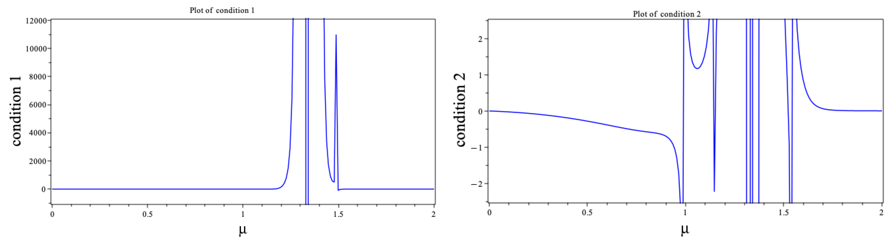
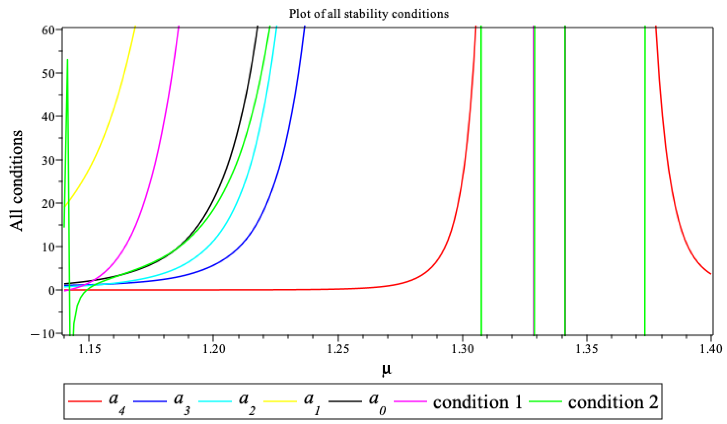
3.2.5. Stability Analysis of $E_4$

First, we require a positive equilibrium point, that is, $G^{\ast }>0,C^{\ast }>0,U^{\ast }>0,I^{\ast }>0$. To guarantee this, the following conditions must hold

• $G^{\ast }>0$ if $G^{\ast }={\displaystyle \frac{\sqrt{B}+Y\beta -h\mu r_2\xi }{X}}>0$ that is, $B>{(h\mu r_2\xi -Y\beta )}^2$,
• $C^{\ast }>0$ if
  $C^{\ast }=-{\displaystyle \frac{r_1(\sqrt{B}+Y\beta -h\mu r_2\xi -K_{1}X)(a\beta \sqrt{B}+aY{\beta }^2-a\beta h\mu r_2\xi +X)}{X^2{K}_1\beta }}>0$ or
  $C^{\ast }={\displaystyle \frac{r_1(\sqrt{B}+Y\beta -h\mu r_2\xi -K_{1}X)(a\beta \sqrt{B}+aY{\beta }^2-a\beta h\mu r_2\xi +X)}{X^2{K}_1\beta }}<0$ that is,
  $r_1(\sqrt{B}+Y\beta -h\mu r_2\xi -K_{1}X)(a\beta \sqrt{B}+aY{\beta }^2-a\beta h\mu r_2\xi +X)<0$ since $X^2{K}_1\beta >0$,
• $U^{\ast }>0$ if
  $U^{\ast }={\displaystyle \frac{h\mu r_2\xi -M\beta K_{2}Nh+a\beta p{r}_2{r}_4-\sqrt{B}}{2h\beta r_{2}M}}>0$ that is,
  ${\left(h\mu r_2\xi -M\beta K_{2}Nh+a\beta p{r}_2{r}_4\right)}^2>B$,
• $I^{\ast }>0$ if
  $I^{\ast }=-{\displaystyle \frac{r_1(\sqrt{B}+Y\beta -h\mu r_2\xi -K_{1}X)(\beta M\sqrt{B}+MY{\beta }^2-h\mu r_2\xi M\beta +\mu X)}{X^{2}p\beta K_1}}>0$ or
  $I^{\ast }={\displaystyle \frac{r_1(\sqrt{B}+Y\beta -h\mu r_2\xi -K_{1}X)(\beta M\sqrt{B}+MY{\beta }^2-h\mu r_2\xi M\beta +\mu X)}{X^{2}p\beta K_1}}<0$ that is,
  $r_1(\sqrt{B}+Y\beta -h\mu r_2\xi -K_{1}X)(\beta M\sqrt{B}+MY{\beta }^2-h\mu r_2\xi M\beta +\mu X)<0$ since $X^{2}p\beta K_1>0$.

Stability analysis of $E_4$ with one free parameter

The expressions of $G^{\ast },C^{\ast },U^{\ast },I^{\ast }$ for $E_4$ strongly depend on the thirteen parameters of model (2). To study the local stability of $E_4$, we rely on finding the eigenvalues of the Jacobian matrix (4) evaluated at $E_4$. Even using a powerful mathematical software such as Maple (latest v. 2024.1), it was not possible to compute all the eigenvalues. Moreover, finding the associated characteristic polynomial to be able to use Routh–Hurwitz criteria is computationally intractable. This is mainly due to the strong dependence of $E_4$ on the thirteen parameters of model 2. Thus, due to the complexity in explicitly analyzing the eigenvalues of $E_4$ and stability conditions, all parameters were kept fixed while one was kept free. This process was iteratively done for all parameters of model (2). Even by keeping one parameter free, the stability analysis is complex. However, the most tractable case was leaving $\mu$ as the free parameter. The stability analysis requires determining the range(s) of values for $\mu$ for which $G,C,U,I>0$ and that at the same time satisfy the Routh–Hurwitz stability criteria for a fourth-order polynomial [81]. In Appendix A, the details of this analysis process are presented with more details. The steps of the analysis are given as follows:

(a)

Fixed parameters values for $r_1,r_2,r_4,a,h,p,\kappa ,\varphi ,\xi ,\beta ,K_1,K_2$ and kept $\mu$ free.

(b)

The Jacobian (4) was evaluated at the equilibrium point $E_4$ and the corresponding characteristic polynomial was analyzed using the Routh–Hurwitz stability criteria to ascertain the interval for $\mu$ where the stability criteria is satisfied.

(c)

Find the Routh–Hurwitz stability criteria in terms of $\mu$ by using the polynomial $P(s,\mu )=a_4{s}^4+a_3{s}^3+a_2{s}^2+a_{1}s+a_0$. In this case, the Routh–Hurwitz stability criteria requires

• $a_i>0$ for $i=0,1,2,3,4$.
• Condition 1: ${\displaystyle \frac{a_2{a}_3-a_1{a}_4}{a_3}}>0$.
• Condition 2: ${\displaystyle \frac{a_1{a}_2{a}_3-a_1^2{a}_4-a_0{a}_3^2}{a_2{a}_3-a_1{a}_4}}>0$.

(d)

The stability conditions are visualized by plots due to the complexity of the conditions.

The conditions for a Hopf bifurcation to arise require that at least one of the previous stability conditions is not met, and at the same time, that at least the real parts of a pair of complex eigenvalues ${\lambda }_{i,j}$ become zero.

3.2.6. Stability Analysis of $E_5$

First, we require a positive equilibrium point, that is, $G^{\ast }>0,C^{\ast }>0,U^{\ast }>0,I^{\ast }>0$. To guarantee this, the following conditions must hold for $E_5=(G^{\ast },C^{\ast },U^{\ast },I^{\ast })$,

• $G^{\ast }>0$ if $G^{\ast }={\displaystyle \frac{-\sqrt{B}+Y\beta -h\mu r_2\xi }{X}}>0$ that is, ${(Y\beta -h\mu r_2\xi )}^2>B$.
• $C^{\ast }>0$ if
  $C^{\ast }=-{\displaystyle \frac{r_1(-\sqrt{B}+Y\beta -h\mu r_2\xi -K_{1}X)(-a\beta \sqrt{B}+aY{\beta }^2-a\beta h\mu r_2\xi +X)}{X^2{K}_1\beta }}>0$ or
  $C^{\ast }={\displaystyle \frac{r_1(-\sqrt{B}+Y\beta -h\mu r_2\xi -K_{1}X)(-a\beta \sqrt{B}+aY{\beta }^2-a\beta h\mu r_2\xi +X)}{X^2{K}_1\beta }}<0$ that is,
  $r_1(-\sqrt{B}+Y\beta -h\mu r_2\xi -K_{1}X)(-a\beta \sqrt{B}+aY{\beta }^2-a\beta h\mu r_2\xi +X)<0$ since $X^2{K}_1\beta >0$.
• $U^{\ast }>0$ if
  $U^{\ast }={\displaystyle \frac{h\mu r_2\xi -M\beta K_{2}Nh+a\beta p{r}_2{r}_4+\sqrt{B}}{2h\beta r_{2}M}}>0$ that is,
  $B>{\left(M\beta K_{2}Nh-h\mu r_2\xi -a\beta p{r}_2{r}_4\right)}^2$.
• $I^{\ast }>0$ if
  $I^{\ast }=-{\displaystyle \frac{r_1(-\sqrt{B}+Y\beta -h\mu r_2\xi -K_{1}X)(-\beta M\sqrt{B}+MY{\beta }^2-h\mu r_2\xi M\beta +\mu X)}{X^{2}p\beta K_1}}>0$ or
  $I^{\ast }={\displaystyle \frac{r_1(-\sqrt{B}+Y\beta -h\mu r_2\xi -K_{1}X)(-\beta M\sqrt{B}+MY{\beta }^2-h\mu r_2\xi M\beta +\mu X)}{X^{2}p\beta K_1}}<0$ that is,
  $r_1(-\sqrt{B}+Y\beta -h\mu r_2\xi -K_{1}X)(-\beta M\sqrt{B}+MY{\beta }^2-h\mu r_2\xi M\beta +\mu X)<0$ since $X^{2}p\beta K_1>0$.

Stability analysis of $E_5$ with one free parameter

The stability analysis of $E_5$ is similar to that of $E_4$. To study the local stability of $E_5$, we rely on finding the eigenvalues of the Jacobian matrix (4) evaluated at $E_5$. Again, finding the associated characteristic polynomial is computationally intractable, due to the strong dependence of $E_5$ on the thirteen parameters of model (2). Thus, we proceed in a similar way to the stability analysis of $E_4$. The details of the analysis are presented in Appendix A. The next section is devoted to the numerical results that support the previous theoretical findings regarding the stability analysis and Hopf bifurcations.

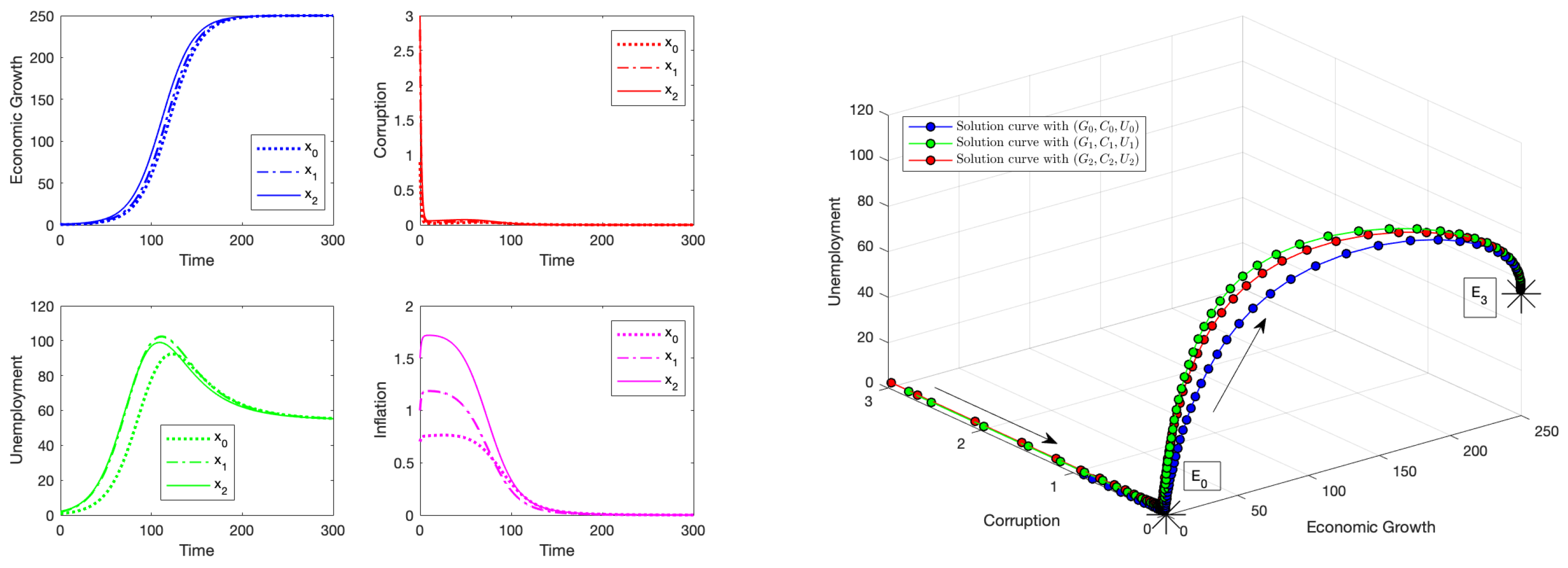
4. Numerical Results

In this section, numerical simulations are carried out in order to analyze the stability of the equilibrium points. These simulations will depict the dynamics of economic growth, corruption, unemployment, and inflation. This will provide additional insight into the dynamics and understanding of the relationship between economic growth, corruption, unemployment, and inflation.

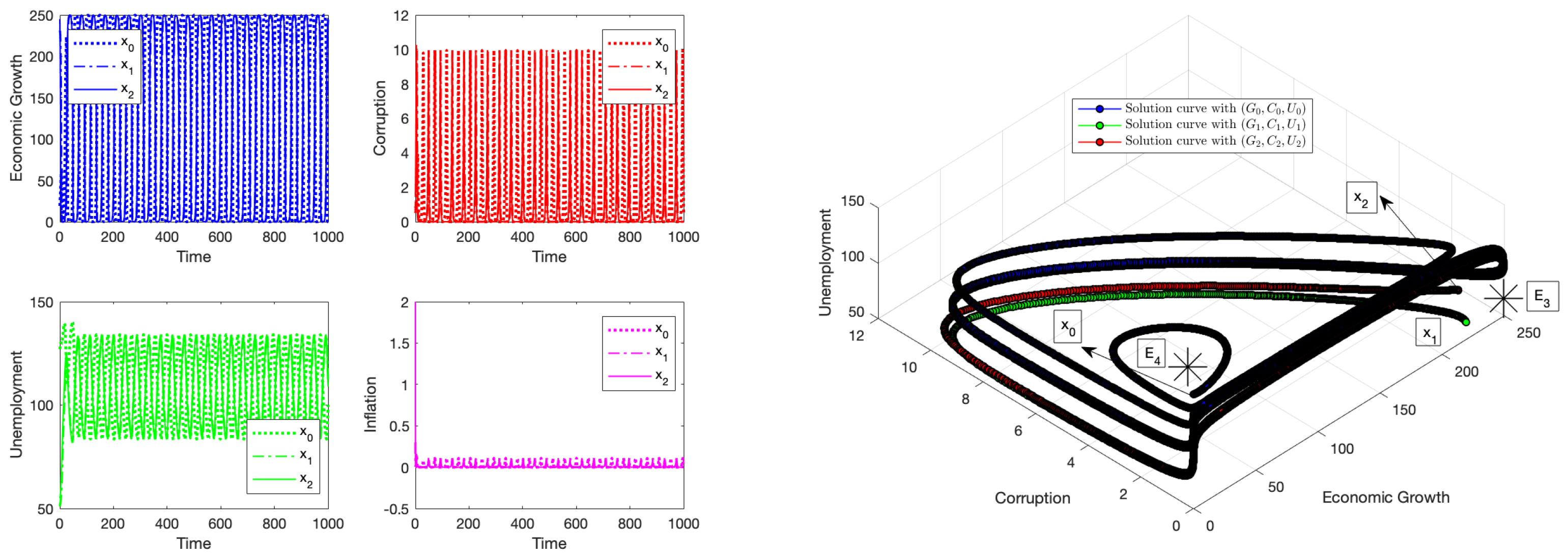
4.1. Numerical Simulation: Instability of the Equilibrium Point $E_0$

Example 1. 

We perform numerical simulations to support the theoretical results that showed that $E_0$ is always unstable. Recall that $E_0=(0,0,0,0)$ is an exterior equilibrium point and is always unstable. Note that the steady state $E_0$ does not represent an ideal state in any economy. It depicts a state with depleted or no economic resources, corruption, unemployment, and inflation [72].

We use different initial conditions relatively close to $E_0$ and the following numerical values for the parameters: $r_1=0.059,r_2=0.0618,\xi ={\displaystyle \frac{1}{3}},\varphi =0.77,K_1=250,K_2=150,\mu =1.005,\kappa =0.005,a=1.25,\beta =0.51,p=0.025,r_4=0.051,h=0.0005$. Figure 1 shows different numerical solutions by varying the initial conditions very close to $E_0$. Begins with a minimal or complete absence of economic growth, corruption, unemployment, and inflation. It can be seen that the solutions diverge from the equilibrium point $E_0$ as expected from the theoretical analysis. In particular, the solutions converge to the equilibrium point $E_3=(250,0,54,0)$ whose eigenvalues are all negative with the aforementioned parameters. Thus, the perturbations of initial values close to $E_0$ will diverge away from it, then $E_0$ is always unstable. From an economic viewpoint, this means that, in a scenario that is very close to the absence of corruption, unemployment, inflation, and economic growth, the system would move away from that situation and move towards the presence of economic growth and unemployment.

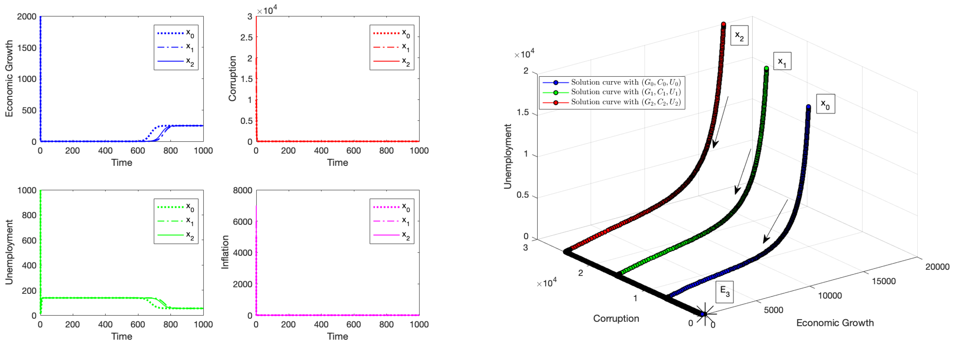
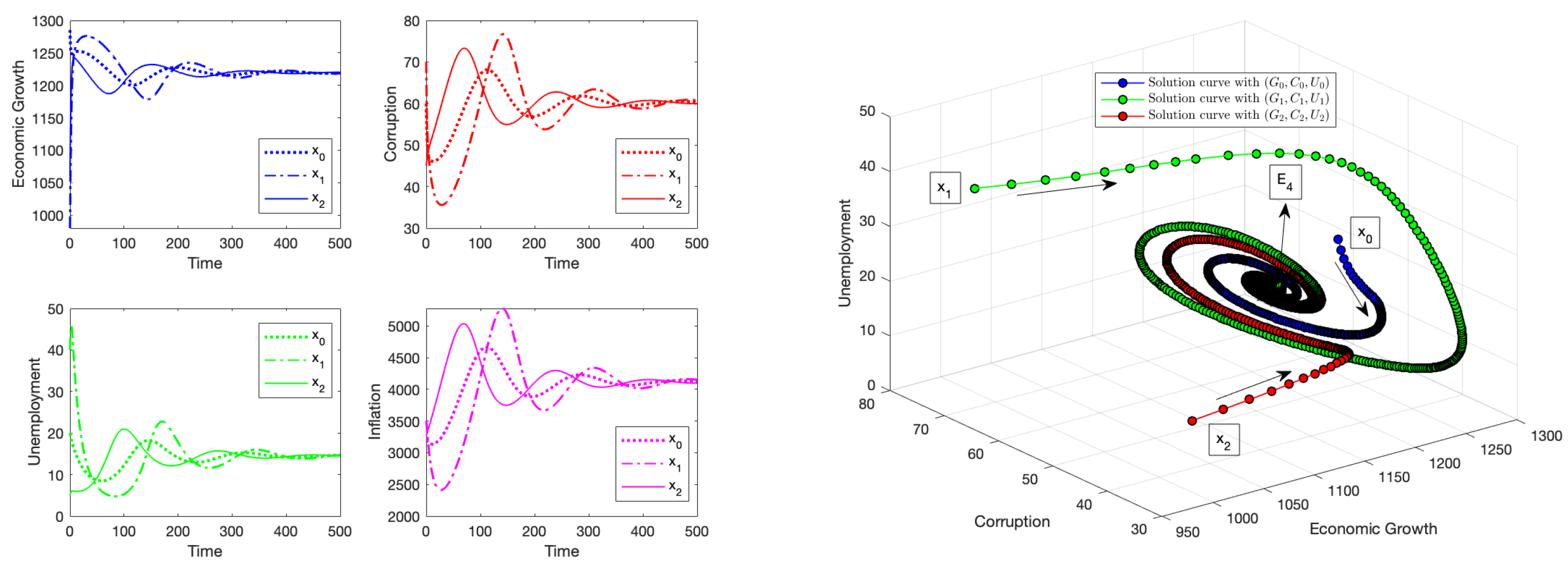
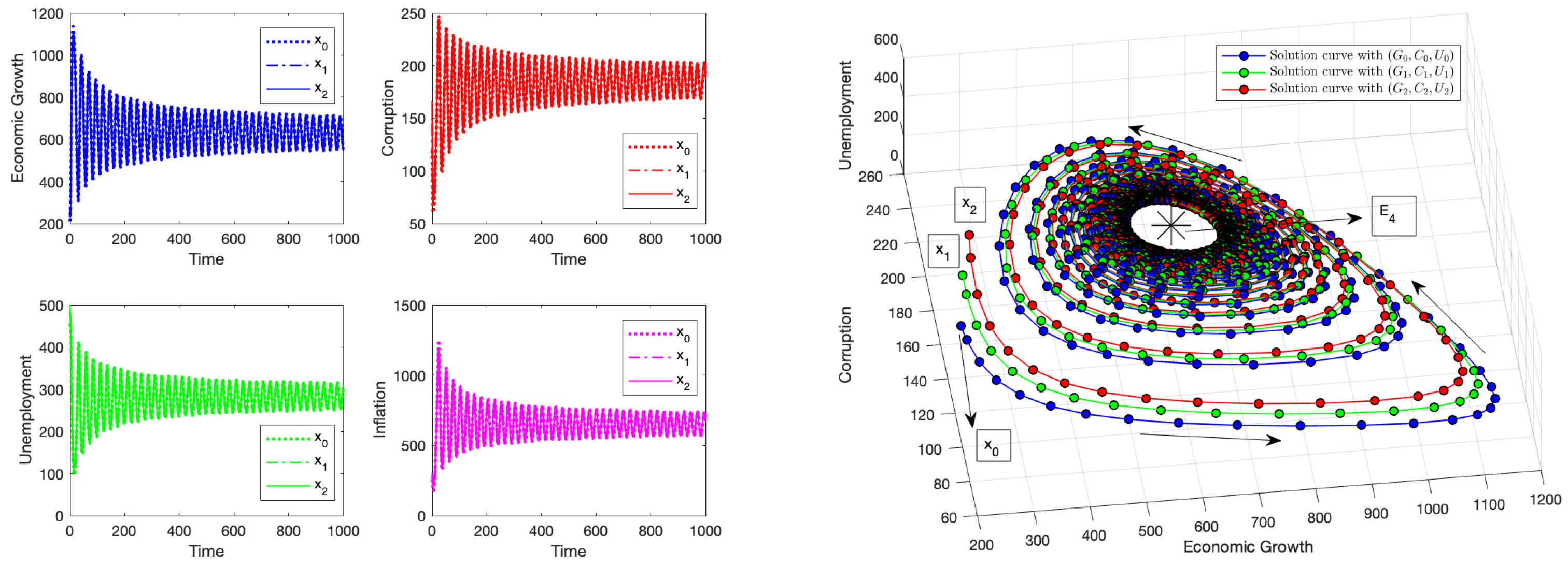
4.2. Numerical Simulation: Instability of the Equilibrium Point $E_1$

Example 2. 

Now, we perform numerical simulations to support the theoretical results that showed that $E_1$ is always unstable. Recall that $E_1=\left(0,0,{\displaystyle \frac{{\mathit{K}}_{\mathit{2}}\left({\mathit{r}}_{\mathit{2}}-\kappa \right)}{{\mathit{r}}_{\mathit{2}}}},0\right)$, which is an axial equilibrium point.

We start the numerical simulations with initial conditions relatively close to $E_1$. We choose the following numerical values for the parameters: $r_1=0.059,r_2=0.121,\xi ={\displaystyle \frac{1}{3}},\varphi =0.1547,K_1=250,K_2=150,\mu =0.5,\kappa =0.05,a=0.85,\beta =0.901,p=0.025,r_4=0.2918,h=0.001$. With these parameters, one obtains that $E_1=(0,0,88.02,0)$.

The eigenvalues of the Jacobian (4) evaluated at $E_1$ are ${\lambda }_1=0.0590,{\lambda }_2=-0.0710,{\lambda }_3=-0.5170,{\lambda }_4=-0.0710.$ Figure 2 shows the numerical solutions with initial conditions relatively close to $E_1$. It can be seen that the solutions go away from $E_1$ but approach $E_4$ as $t\to \infty$. Thus, this provides additional support for the fact that $E_1$ is always unstable. This nature of $E_1$ is also not an ideal state in any economy. Having a certain level of unemployment with the complete absence of economic growth, corruption, and inflation is not sustainable in the long run. In other words, the instability of $E_1$ means that in a scenario close to the absence of corruption, inflation, and economic growth, but with unemployment, the system would move away from that situation.

4.3. Numerical Simulation: Instability of the Equilibrium Point $E_2$

Example 3. 

We perform numerical simulations to support the theoretical results that have proved that $E_2$ is always unstable regardless of the numerical values of the parameters ($\kappa <r_2$). Recall that $E_2=({\mathit{K}}_{\mathit{1}},0,0,0)$ is an axial equilibrium point. We start the numerical simulations with initial conditions very close to $E_2$. For these numerical simulations, we use the values of the parameters $r_1=0.059,r_2=0.121,\xi ={\displaystyle \frac{1}{3}},\varphi =0.1547,K_1=250,K_2=150,\mu =0.5,\kappa =0.05,a=0.85,\beta =0.901,p=0.025,r_4=0.2918,h=0.001$. Thus, one obtains the equilibrium point $E_2=(250,0,0,0)$. With these values, the eigenvalues of the Jacobian (4) evaluated at $E_2$ are

$$\begin{array}{cc}\hfill {\lambda }_1& =-r_1=-0.059<0,\hfill \\ \hfill {\lambda }_2& ={\displaystyle \frac{-\left((a\mu -\varphi )K_1\beta +\mu \right)+\sqrt{{\left((a\mu -\varphi )K_1\beta +\mu \right)}^2+4p{r}_4{\left(K_{1}a\beta +1\right)}^2}}{2(K_{1}a\beta +1)}}=0.0214>0,\hfill \\ \hfill {\lambda }_3& ={\displaystyle \frac{-\left((a\mu -\varphi )K_1\beta +\mu \right)-\sqrt{{\left((a\mu -\varphi )K_1\beta +\mu \right)}^2+4p{r}_4{\left(K_{1}a\beta +1\right)}^2}}{2(K_{1}a\beta +1)}}=-0.3404<0,\hfill \\ \hfill {\lambda }_4& =-{\displaystyle \frac{{\mathit{K}}_{\mathit{1}}{\mathit{r}}_{\mathit{2}}\xi +\left(\kappa -{\mathit{r}}_{\mathit{2}}\right){\mathit{K}}_{\mathit{2}}}{{\mathit{K}}_{\mathit{2}}}}=-0.0038<0.\hfill \end{array}$$

From the theoretical analysis performed in the previous section, it was found that the eigenvalue ${\lambda }_2$ is always positive and, therefore, $E_2$ is always unstable. Figure 3 shows that the solutions do not converge to $E_2$, but rather to $E_4$.

The steady state $E_2$ is a good economic scenario. However, an economy can only reach maximum economic growth, no corruption, no unemployment, and no inflation when it functions at its maximum output of resources, which means that it utilizes all available resources efficiently, with a stable political system that prevents corruption, and a well-managed monetary policy to control inflation, while maintaining a healthy labor market with minimal unemployment [82]. But in practice, achieving this state is very difficult and almost unattainable due to diverse complex economic factors. Thus, starting out close to this state, the system will move away from this in the long run. In other words, the instability of $E_2$ means that in a scenario close to the absence of corruption, inflation, and unemployment, but with economic growth, the system would move away from that scenario.

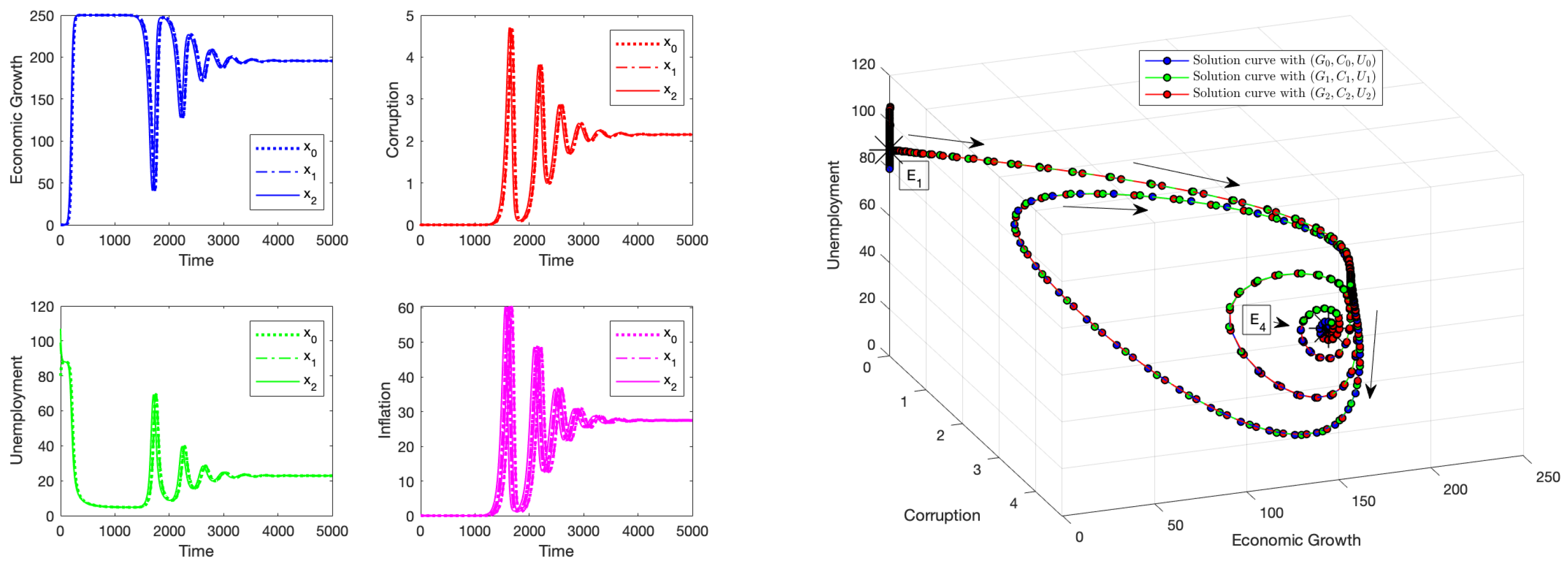
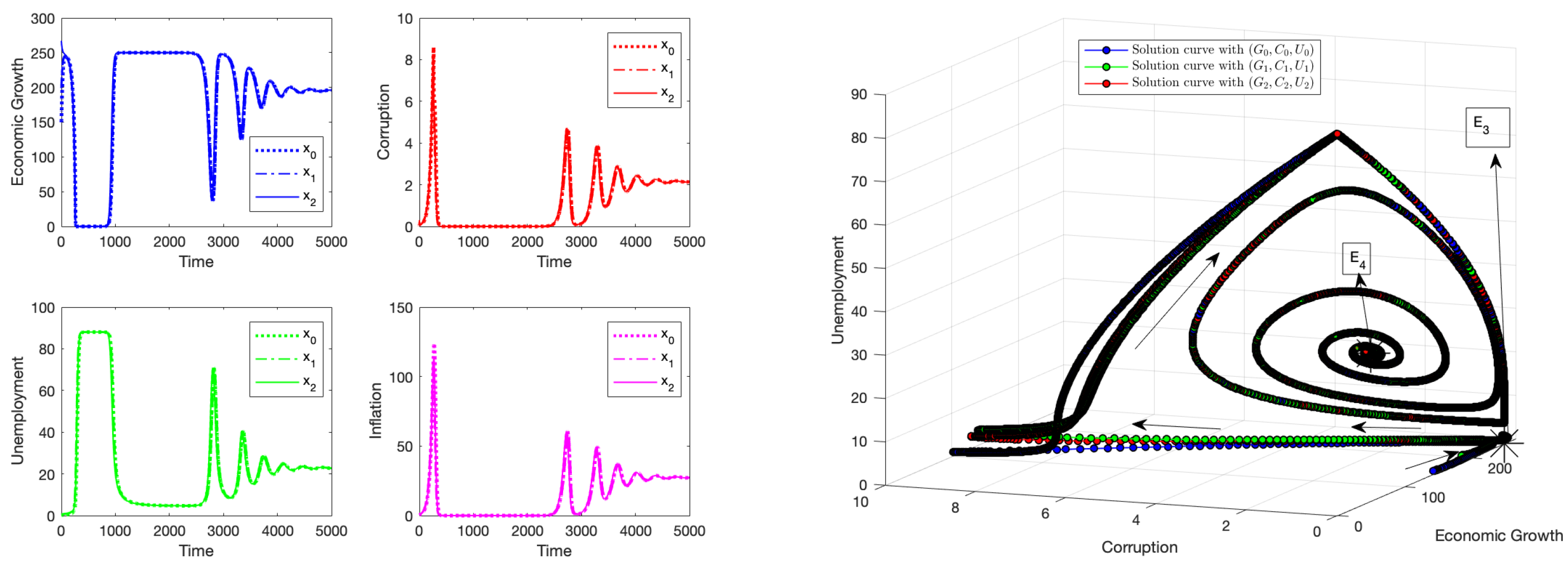
4.4. Numerical Results Related to the Stability of Equilibrium Point $E_3$

To support the theoretical results of the analysis of the equilibrium point $E_3$, we perform numerical simulations to show that $E_3$ is locally stable under some conditions that depend on the parameters. Recall that $E_3=\left({\mathit{K}}_{\mathit{1}},0,-{\displaystyle \frac{{\mathit{K}}_{\mathit{1}}{\mathit{r}}_{\mathit{2}}\xi +\kappa {\mathit{K}}_{\mathit{2}}-{\mathit{K}}_{\mathit{2}}{\mathit{r}}_{\mathit{2}}}{{\mathit{r}}_{\mathit{2}}}},0\right)$.

Example 4. 

For the numerical simulations, we use the following values for the parameters: $r_1=0.059,r_2=0.0618,\xi ={\displaystyle \frac{1}{3}},\varphi =0.77,K_1=250,K_2=150,\mu =1.005,\kappa =0.05,a=1.25,\beta =0.51,p=0.025,r_4=0.051,h=0.125$. We vary the initial conditions to provide additional support for the theoretical analysis and to numerically investigate the global stability of the equilibrium point $E_3$.

With the aforementioned numerical values for the parameters, one obtains $E_3=(250,0,54.531,0)$. Moreover, computing the Routh–Hurwitz stability conditions and the eigenvalues of the Jacobian (4) evaluated at $E_3$, one obtains

$${\lambda }_1=-0.059<0,{\lambda }_2=-0.0225<0,c_1=0.07535>0,c_0=0.000036>0.$$

Also, from the second stability requirement of Theorem 5, one has ${\displaystyle \frac{K_1{r}_2\xi +(\kappa -r_2)K_2}{K_2}}=-0.0225<0$. Thus, all the stability conditions are satisfied. Therefore, $E_3$ is locally asymptotically stable.

Figure 4 shows the numerical solution of system (2) by using different initial conditions. These results support the theoretical results regarding the local stability of $E_3$ when the conditions of Theorem 5 are met. If the initial values are close to $E_3$, the system (2) will converge to $E_3$ as time evolves. The equilibrium $E_3$ represents a state with a certain level of unemployment, zero corruption, and inflation brought about by maximizing economic resources fairly efficiently. With cautionary policies in place to curb corruption and inflation, and maintain unemployment at a certain level while operating at full economic capacity, this can be ideal, but it will take a lot of effort to achieve.

The steady state $E_3$ also depicts a scenario in which crucial efforts are made to maximize economic resources that can lead to avoiding corruption and inflation, but still with unemployment. There is the positive utilization of resources, and as such, more efforts should be geared toward creating more job vacancies. Thus, establishing job innovation ideas, entrepreneurship workshops, and other job programs will eventually decrease unemployment while continuously maintaining anti-corruption and inflation measures at a sustainable level. Thus, starting relatively close to this state and under stability conditions, any small perturbation will cause the system to return to $E_3$ as time evolves.

Figure 5 shows the numerical solution of system (2) using the different initial conditions that are relatively distant from $E_3$. This is to numerically explore the global stability of $E_3$, although a theoretical approach will guarantee this feature. The numerical simulations suggest the global stability of $E_3$ when the conditions of Theorem 5 are met.

Example 5. 

The stability of $E_3$ depends on certain stability conditions that must be met. However, if one of the stability requirements for $E_3$ is not met, the equilibrium point becomes unstable. Thus, regardless of the initial conditions, the solutions of system (2) will not approach $E_3$. Using the following parameters: $r_1=0.69,r_2=0.11,r_4=0.678,K_1=250,K_2=150,\xi ={\displaystyle \frac{1}{3}},\varphi =0.08,\mu =0.9,\kappa =0.001,a=0.05,\beta =1,h=0.71,p=0.671$. With these new values, one obtains $E_3=(250,0,65.30,0)$, $c_1=45.78>0$, $c_0=-27.42<0$. We see that one stability requirement is not met since $c_0<0$. The eigenvalues of the Jacobian (4) evaluated at $E_3$ are ${\lambda }_1=-0.69<0,{\lambda }_2=-0.0479<0,{\lambda }_3=0.5912>0$, and ${\lambda }_4=-46.3748<0$. Since $E_3$ is unstable, the solution trajectories will diverge from it. With regard to the eigenvalues of the Jacobian (4) evaluated at $E_4$, one obtains ${\lambda }_1=-99.5209,{\lambda }_2=-0.1028,{\lambda }_{3,4}=0.1384\pm 0.4746i$. Thus, $E_4$ is unstable, and the solutions will not converge to it. Figure 6 shows that the solutions do not approach $E_3$ or $E_4$. It can be seen that there is a Hopf bifurcation arising from $E_4$, which we will analyze in the next section.

4.5. Numerical Results Related to the Stability of Equilibrium Point $E_4$

In Section 3.2.5, we found general conditions for the local stability of $E_4$ in terms of the parameter $\mu$. The interior equilibrium points $E_4$ and $E_5$ depend on $\mu$. Thus, the associated characteristic polynomials also strongly depend on $\mu$. To support the theoretical and computational analysis of the local stability of $E_4$ (see Appendix A), we obtain the numerical solutions of system (2). We fix the following values of the parameters, $r_1=0.69,r_2=0.87,\xi =0.455,\varphi =0.9,K_1=1350,K_2=570,\kappa =0.001,a=0.671,\beta =0.0119,p=0.01,r_4=0.99,h=0.001$, and keep $\mu$ free. With these parameters, we obtain the ranges of $\mu$ in which $E_4$ is locally asymptotically stable and also where the components of $E_4$ are positive. The intervals are $1.154\le \mu \le 1.307$ and $1.65\le \mu \le 2$ (see Figure A1 and Figure A5 in Appendix A).

Example 6. 

The equilibrium point $E_4$ is approximately $E_4=(1219.48,60.19,14.48,4114.99)$ when $\mu =1.9$. However, $E_5$ has some negative components and then does not represent a real-world scenario. In this scenario, $E_4$ represents good economic growth (since $K_1=1350$), reduced unemployment (since $K_2=570$), the presence of corruption, and inflation. This depicts a demand–pull type of inflation that occurs when demand for goods and services (which is a direct effect of this good economic growth) surpasses supply, leading to an increase in prices [83]. There is substantial economic growth and expansion present. This economic growth can lead to an increase in the buying habits of goods and services by consumers, leading to the demand for more goods and services. From the law of demand and supply, as demand increases, supply may decrease, giving rise to inflated prices of goods and services, causing inflation to rise. The conditions for stability all stem from an intricate relationship between the parameters, all delicate, and each one of them has to be met. This shows the difficulty in achieving this state $E_4$ in the real world, but it is feasible and attainable. Thus, the role of inflation in this system cannot be overemphasized, since the corruption and unemployment levels are maintained by the coexisting relationship with economic growth and inflation.

The real part of all the eigenvalues of the Jacobian matrix (4) evaluated at $E_4$ are negative with a pair of complex eigenvalues. Thus, $E_4$ is locally asymptotically stable. Figure 7 shows different numerical solutions for various initial conditions, all of which are somewhat close to $E_4$. It can be observed that the numerical solutions proceed toward $E_4$ as time evolves.

Example 7. 

Next, we take initial values far from $E_4$ to numerically explore the global stability of $E_4$, although a theoretical proof that might involve Lyapunov functions can guarantee this. Using the same values of the parameters as before but with $K_1=1250$, one obtains $E_4=(1219.48,15.20,14.48,1039.20)$, and again $E_5$ is unrealistic. In this scenario, all the eigenvalues are complex with negative real parts. Figure 8 shows the numerical solutions of system (2) with different initial conditions that are relatively far from $E_4$. As can be seen, all the solutions approach $E_4$, and this suggests that $E_4$ is globally asymptotically stable.

Example 8. 

Let us proceed to explore the qualitative behavior of the solutions of system (2) when the equilibrium point $E_4$ is unstable. To make $E_4$ unstable, we have many alternatives. Let us reduce μ from $1.9$ to $1.153$. Note that $1.153\notin \left\{[1.154,1.307]\cup [1.65,2]\right\}$, which are the stability intervals for the parameter μ. However, in order to prove that a Hopf bifurcation occurs, we will need to find the value of μ such that $\lambda =\pm i\omega$ are eigenvalues of the Jacobian (4) evaluated at $E_4$ and check that the transversality condition is satisfied. From the associated characteristic polynomial, it can be seen that finding the eigenvalues is computationally intractable (see Appendix A). Now, using the same parameter values as in Example 6 but with $\mu =1.153$, one obtains $E_4=(627.48,186.52,283.84,650.55)$ and $E_5$ is unrealistic. All the eigenvalues of the Jacobian (4) evaluated at $E_4$ are complex. One pair of eigenvalues has positive real parts. Thus, $E_4$ is no longer locally asymptotically stable. Moreover, by continuation, we can deduce that there is a ${\mu }_0$ such that $\lambda =\pm i\omega$ are eigenvalues and the transversality condition is satisfied. Figure 9 shows numerical solutions with different initial conditions. As can be seen, the solutions do not approach $E_4$ but approach a limit cycle around $E_4$. This depicts a Hopf bifurcation arising from the complex eigenvalues ${\lambda }_1$ and ${\lambda }_2$ crossing from the ${\mathbb{C}}^{-}$ plane to the ${\mathbb{C}}^{+}$ plane. The limit cycle obtained here represents periodic fluctuations in the socioeconomic system (2) where it repeatedly oscillates between different levels of economic growth, corruption, unemployment, and inflation, but without approaching $E_4$. These economic limit cycles are common in economic systems [34,84,85].

Example 9. 

Next, we will show that the Hopf bifurcation still occurs when the parameter μ is far from the stability set $\left\{[1.154,1.307]\cup [1.65,2]\right\}$. Let us take $\mu =0.87$. In this case, $E_4=(215.97,130.68,471.08,274.64)$, and in particular, $E_5$ is unrealistic. All the eigenvalues of the Jacobian (4) evaluated at $E_4$ are complex. One pair of eigenvalues has positive real parts. Thus, $E_4$ is not locally asymptotically stable. Figure 10 shows numerical solutions with different initial conditions. As can be seen, the solutions do not approach $E_4$ but approach a limit cycle around $E_4$. This depicts a Hopf bifurcation arising from the complex eigenvalues ${\lambda }_1$ and ${\lambda }_2$ crossing from the ${\mathbb{C}}^{-}$ plane to the ${\mathbb{C}}^{+}$ plane. Again, the limit cycle obtained here represents periodic fluctuations in the socioeconomic system (2) where it repeatedly oscillates between the different levels of economic growth, corruption, unemployment, and inflation, but without converging to $E_4$.

5. Sensitivity Analysis

This section focuses on conducting sensitivity analysis to assess how changes in certain parameter values for this model affect the final output of the system. The aim is to determine which factors have the most significant impact on the system. Sensitivity analysis provides in-depth understanding and insight into the intricate relationships that exist among socioeconomic phenomena. Thus, it will help policymakers make informed and educated decisions that benefit the economy. This paper is primarily focused on the impact inflation that has on economic growth, corruption, and unemployment. Thus, sensitivity analysis on inflation factors is first considered. We will explore sensitivity analysis on the equilibrium points $E_3$ and $E_4$, which are closer to the most realistic scenarios.

5.1. Sensitivity Analysis for $E_3=\left\{G={\mathit{K}}_{\mathit{1}},C=0,U={\displaystyle \frac{{\mathit{K}}_{\mathit{1}}{\mathit{r}}_{\mathit{2}}\xi +\kappa {\mathit{K}}_{\mathit{2}}-{\mathit{K}}_{\mathit{2}}{\mathit{r}}_{\mathit{2}}}{{\mathit{r}}_{\mathit{2}}}},I=0\right\}$

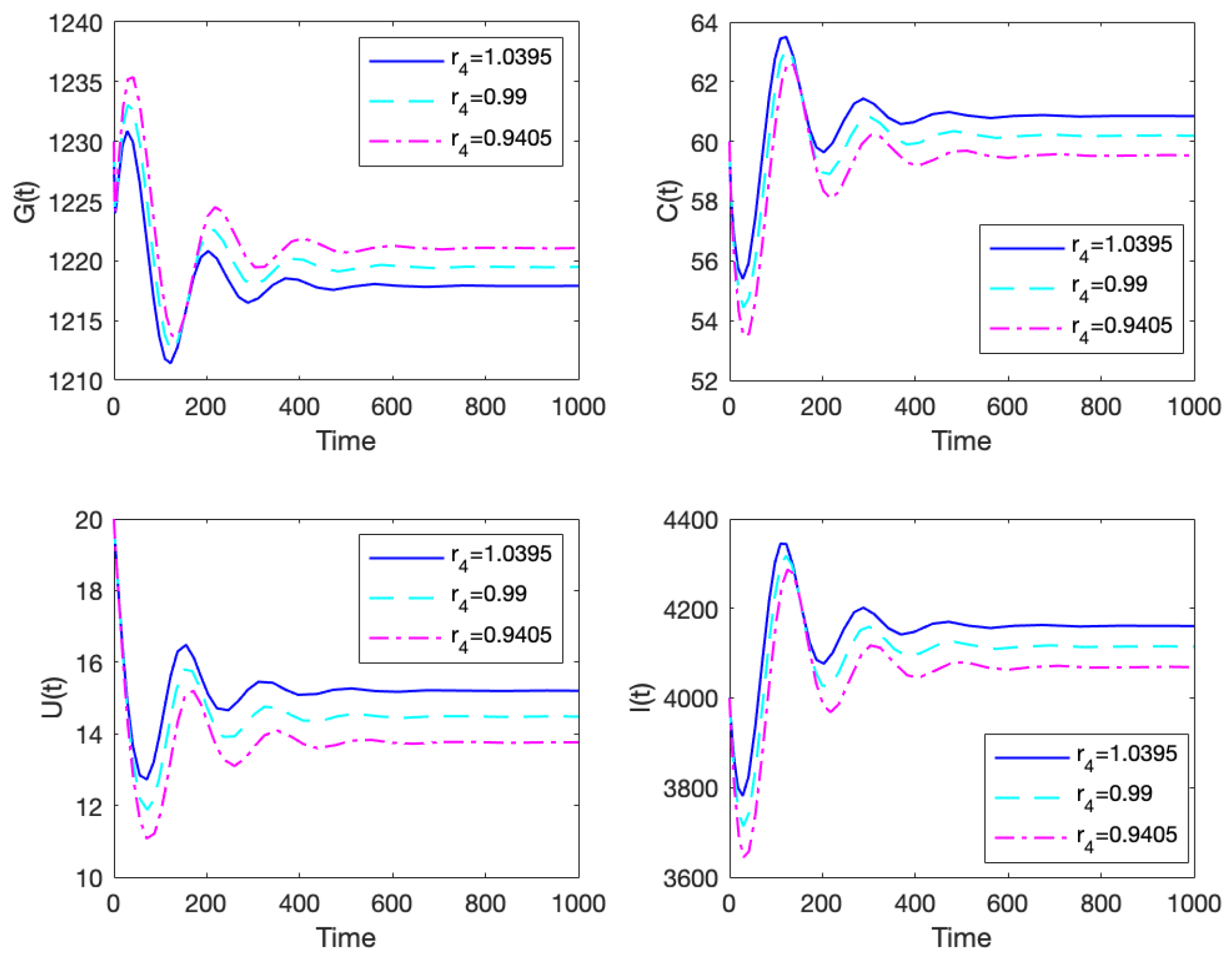
• Effects of Inflation using parameters $r_4$ and h
  Economically and socially, an increase or decrease in inflation affects economic growth, corruption, and unemployment, and it is crucial to study how the increase or decrease in inflation affects these state variables. When a nation sets up adequate policies to curb inflation, it helps the general welfare. These policies are factors that decrease inflation through the parameters h and $r_4$. We will study this effect using $r_4$ and h with a $5\%$ increase and decrease. First, we use the parameter values $r_1=0.059,r_2=0.0618,K_1=250,K_2=150,\xi =1/3,\varphi =0.77,\mu =1.005,\kappa =0.005,a=1.25,\beta =0.51,p=0.025,r_4=0.051$, and $h=0.125$. Figure 11 and Figure 12 show the effect of the variation of the parameters $r_4$ and h on the dynamics of system (2), respectively. It can be observed that variations of $5\%$ to parameters $r_4$ and h do not produce a notable change in the output of system (2). This means that, for the economy to experience a significant reduction in inflation, higher inflation curtailment factors should be enforced. That is, huge increases in the factors that curb inflation are critical in ensuring noteworthy and positive outcomes.
• Effects of corruption using parameter $\mu$
  Next, we investigate how sensitive the system (2) is to corruption by using parameter $\mu$, which represents the factors that directly reduce corruption. We use the parameter values $r_1=0.059,r_2=0.0618,K_1=250,K_2=150,\xi =1/3,\varphi =0.77,\kappa =0.005,a=1.25,\beta =0.51,p=0.025,r_4=0.051,h=0.125$ and vary $\mu$ by $5\%$. Conclusively, Figure 13 shows no notable changes in the system’s output for a $5\%$ variation in the parameter $\mu$.

5.2. Sensitivity Analysis for $E_4=(G^{\ast },C^{\ast },U^{\ast },I^{\ast })$

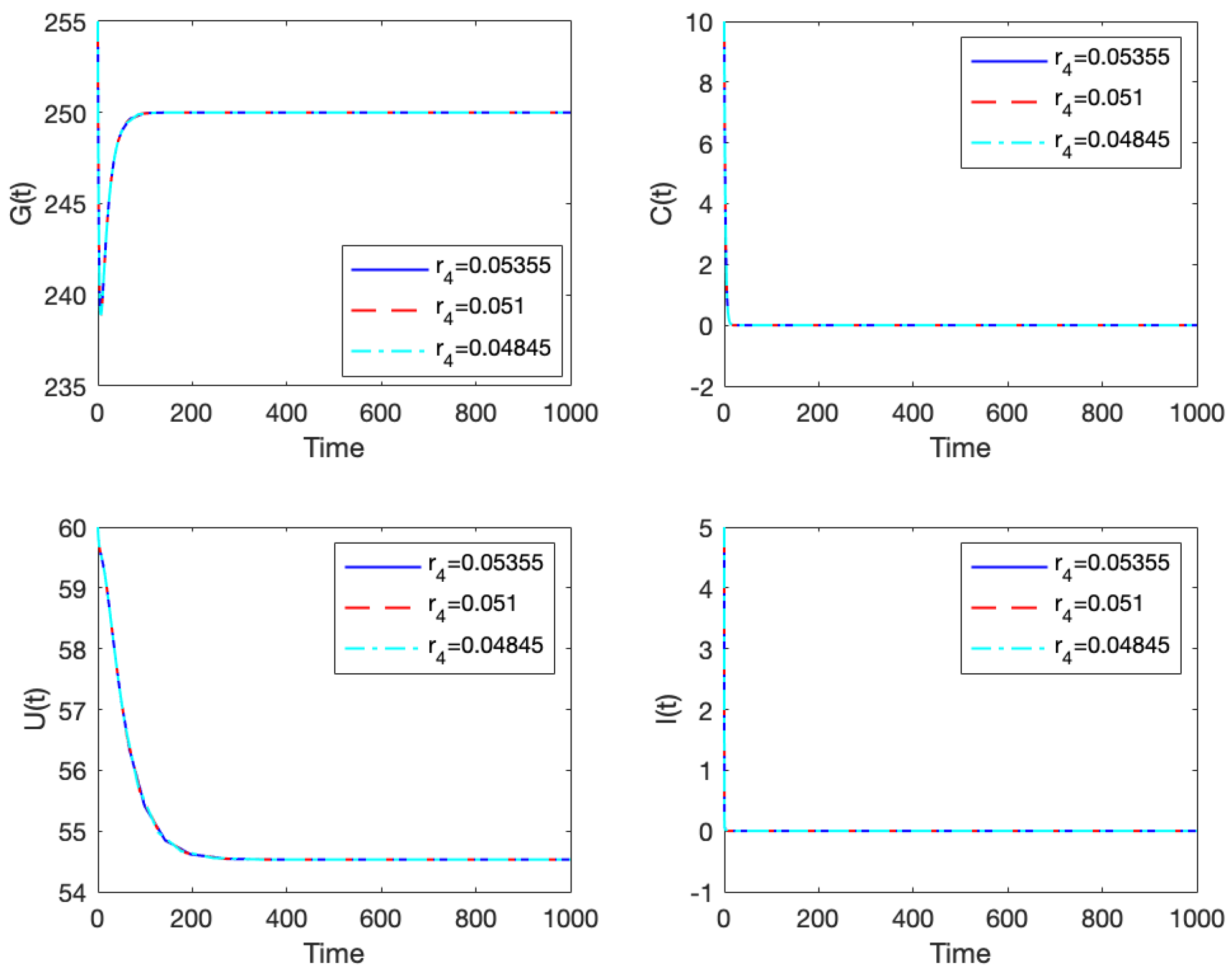
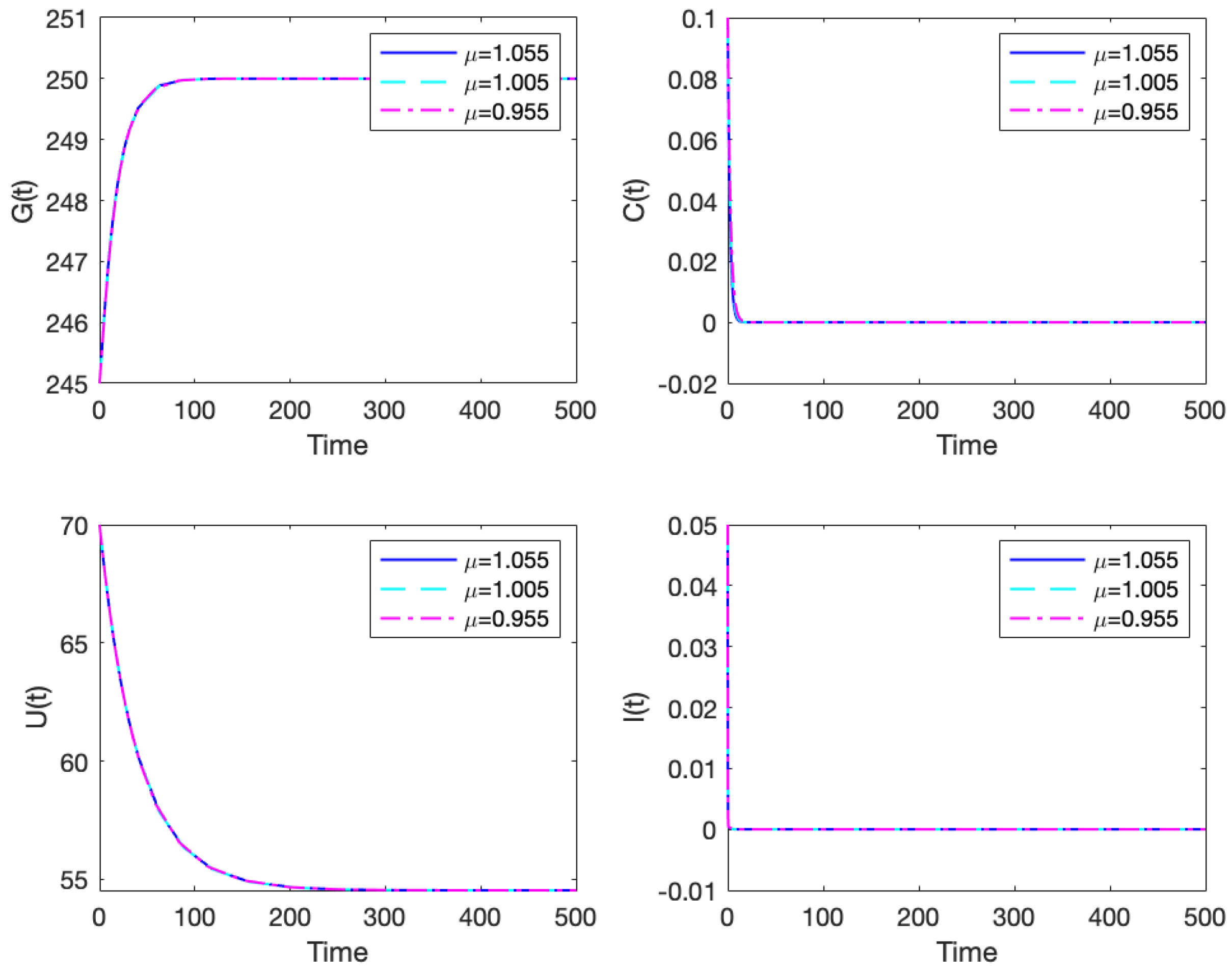
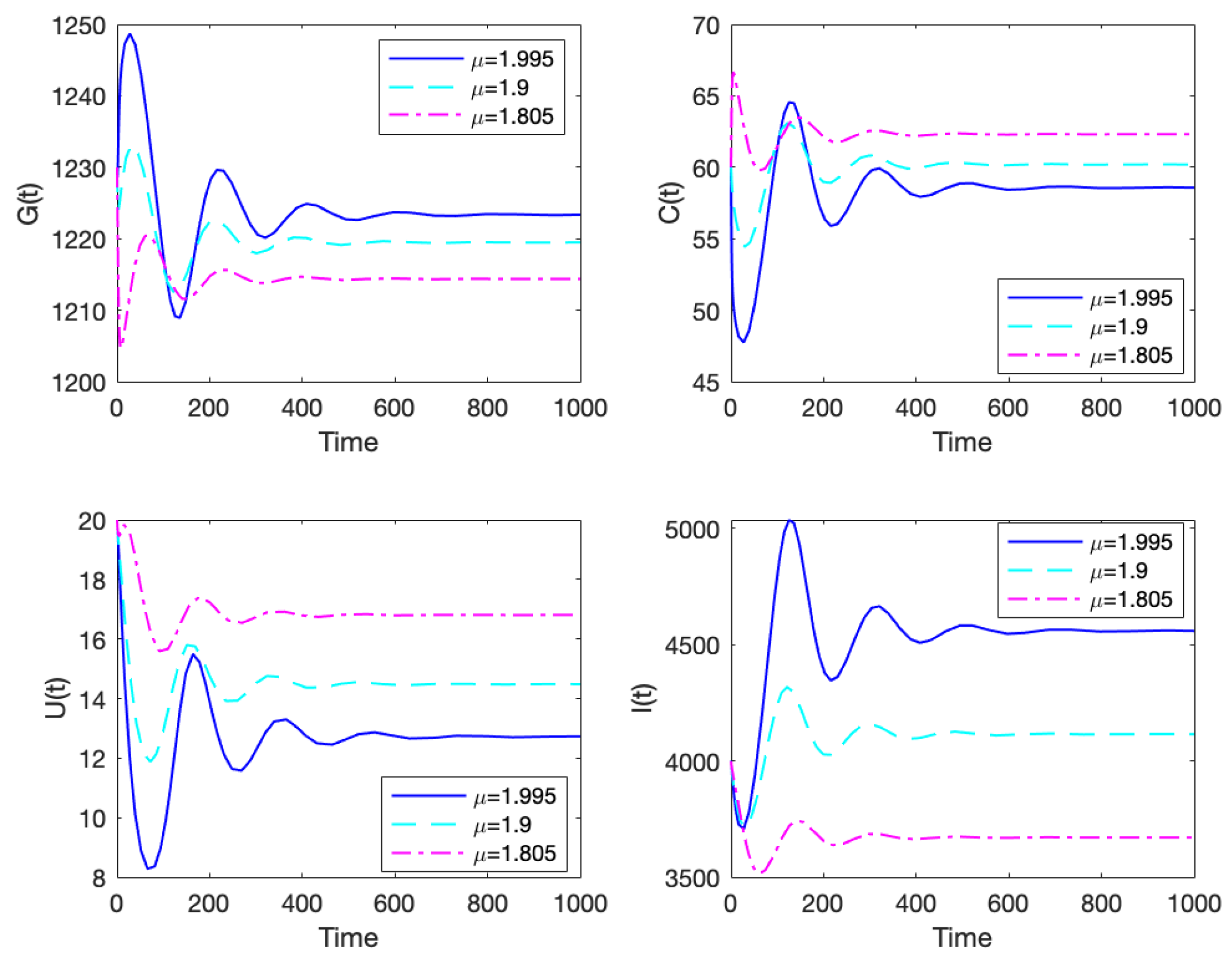
• Effects of Inflation using parameters $r_4$ and h
  This section is devoted to the sensitivity analysis of system (2) for the equilibrium point $E_4$ by varying the input in key parameters of the model. The control of inflation has been the top game for policymakers, especially in recent times. Striving to keep the inflation rate at the required level that promotes economic growth is paramount in any nation’s economy. Research has shown that there can be no positive outcome for economic growth and employment if a nation’s economy is run on high inflation [86]. We use the parameter values $r_1=0.69,r_2=0.87,K_1=1350,K_2=570;\mu =1.9,\xi =0.455,\varphi =0.9,\kappa =0.001,a=0.671,\beta =0.0119,h=0.001,p=0.01$ are used with a $5\%$ variation for $r_4$. Figure 14 shows that even a little $5\%$ variation in $r_4$ produces a significant change in the system. As $r_4$ increases, inflation, corruption, and unemployment increase while economic growth reduces and vice versa. This is a typical scenario seen in several economies around the world. When the cost of goods and services increases, many companies struggle to stay in business, and a direct implication of this is laying off employees, increasing the unemployment rate. Again, these high rates will reduce the demand for goods and services, leading to a reduction in the labor force.
  Next, we investigate the inflation parameter h (factors that directly decrease inflation) using the parameter values $r_1=0.69,r_2=0.87,K_1=1350,K_2=570,\mu =1.9,\xi =0.455,\varphi =0.9,\kappa =0.001,a=0.671,\beta =0.0119,r_4=0.99,p=0.01$ with a $5\%$ variation for h. Figure 15 shows a significant change in the outcome when varying h. As h increases (increase in the factors that directly curb inflation), economic growth improves, corruption and unemployment decline, and vice versa. Thus, for any ideal $E_4$ economic scenario, policymakers should focus on keeping inflation levels in check by establishing and enforcing factors like decreased government spending and money supply, monetary and fiscal policies. For instance, in the USA, the Federal Reserve adjusts the rates in order to control inflation [87,88].
• Effects of Corruption using the parameter $\mu$
  The parameter $\mu$ represents factors that directly reduce corruption, and it is a crucial parameter to study any economic scenario close to $E_4$. Economically and socially, corruption plays a role in the progression or the retrogression of a nation’s economy [89,90]. If there are more factors enforced to curb corruption, a nation’s economic growth will flourish, which in turn aids in the reduction in unemployment, corruption, and inflation rates [89]. We use the parameter values $r_1=0.69,r_2=0.87,K_1=1350,K_2=570,h=0.001,\xi =0.455,\varphi =0.9,\kappa =0.001,a=0.671,\beta =0.0119,r_4=0.99,p=0.01$, with a $5\%$ variation for $\mu$. Figure 16 shows the impact caused by a $5\%$ variation of $\mu$. The system is sensitive to corruption. It tells us that, when there are more factors that aid in corruption reduction, economic growth blossoms, unemployment reduces, inflation increases, and vice versa. Reduced corruption can sometimes lead to a temporary increase in inflation because when a government becomes less corrupt, it often needs to implement new policies and procedures to manage the economy more efficiently, which can disrupt existing market dynamics and lead to short-term price fluctuations, particularly if the government is also trying to increase transparency in pricing mechanisms. Socioeconomic relationships are sometimes not always black and white since there are other sub-socioeconomic phenomena all interwoven in a nation’s economy [91].

6. Discussion and Conclusions

In this paper, we proposed a new mathematical model to explore the dynamics of economic growth, corruption, unemployment, and inflation. The proposed model includes several relationships between these socioeconomic factors that have been proposed and studied by economists. The model presented in this paper can be considered an extension of a previous mathematical model that only considers economic growth, corruption, and unemployment, but not inflation. Thus, in this paper, we studied the impact that inflation has on all of the dynamics. First, we found all potential steady states of the economic system based on the proposed model. Secondly, we performed the local stability analysis of all the steady states in order to investigate the dynamics of the economic system. We found that the proposed model has six equilibrium points. The expressions of two equilibrium points $E_4$ and $E_5$ strongly depend on the thirteen parameters of model (2). To study the local stability of these equilibrium points, we relied on finding the eigenvalues of the Jacobian matrix (4) evaluated at those equilibrium points. However, even using a powerful mathematical software such as Maple, it was not possible to compute all the eigenvalues in terms of the parameters. Furthermore, finding the associated characteristic polynomial to be able to use Routh–Hurwitz criteria is computationally intractable. This is mainly due to the strong dependence of the equilibrium points $E_4$ and $E_5$ on the thirteen parameters of model (2). Thus, due to the complexity in explicitly analyzing the eigenvalues or the characteristic polynomial to analyze the local stability conditions, we kept all parameters fixed while one was kept free. This process was iteratively done for all parameters of the model. However, even by keeping one parameter free, the local stability analysis is complex. Nevertheless, the most tractable case was leaving $\mu$ as the free parameter. Thus, the stability analysis required that the range(s) of values for $\mu$ were determined, for which the components of the equilibrium point $E_4$ were non-negative and at the same time satisfied the Routh–Hurwitz stability criteria. In summary, we found conditions such that the equilibrium point $E_4$ is locally stable in terms of one parameter of the model. In particular, due to the complexity of the stability conditions, we selected the clearance of criminality as the free parameter. However, we also explored the stability conditions in terms of other parameters of the model, where the analyses were even more complex. For the other equilibrium points $E_0$, $E_1$, $E_2$, and $E_3$, we were able to find the general local stability conditions without fixing the values of the parameters. In addition, we were able to numerically find the existence of Hopf bifurcations arising from equilibrium points $E_3$ and $E_4$. However, even with one free parameter, finding the theoretical conditions for the existence of Hopf bifurcations is a challenging task. We performed various numerical simulations that supported the theoretical results. Some corresponding socioeconomic scenarios were discussed. The proposed mathematical model has several limitations. For instance, there are many other factors that can affect the economic growth of a nation. It has been suggested that domestic investment, education, official development assistance, and government effectiveness can affect economic growth [92]. In [93], it was found that the instability of the political regime negatively affects economic growth. Also, it has been found that economic growth is affected by exports, imports, foreign direct investment inflow, foreign direct investment outflow, and social contributions [94]. Including all these previous factors could be very challenging due to the intricate relationships between these variables and the dimension of the potential mathematical model. Another limitation is that the realistic values of the parameters have not been explored, and this aspect can be very challenging. Moreover, panel data for corruption can be very difficult to obtain, and the units to measure it need to be defined. In [95], the authors used panel data and found that labor market and criminal justice strategies are important to reduce crime, which in some way includes corruption [96]. In [97], panel data were used to investigate the effect of corruption on countries’ economic efficiency. The corruption was measured by the corruption perceptions index (CPI), but there are other ways to measure corruption, and it is a complex topic [98,99].

With regard to future research directions that can be explored, additional variables can be added to the model, and different relationships between the variables can be incorporated. From a strictly mathematical viewpoint, the global stability of the steady states can be explored and the application of the Poincaré–Lindstedt perturbation method can be explored to study the stability of the equilibrium point $E_4$ in terms of all the parameters. Finally, the study of Hopf bifurcation often involves considering a time delay as a bifurcation parameter. An open question is to investigate whether time delays can be included to extend the current model and analyze the role of delays in the system’s behavior. This can provide a deeper understanding of the stability of the socioeconomic system.

References

- De la Fuente, A.; De La Fuente, A. Mathematical Methods and Models for Economists; Cambridge University Press: Cambridge, UK, 2000. [Google Scholar]
- Gandolfo, G. Economic Dynamics: Methods and Models; Elsevier: Amsterdam, The Netherlands, 1971; Volume 16. [Google Scholar]
- Hritonenko, N.; Yatsenko, Y. Mathematical Modeling in Economics, Ecology and the Environment; Springer: Berlin/Heidelberg, Germany, 1999. [Google Scholar]
- Morgan, M.S.; Knuuttila, T. Models and modelling in economics. Philos. Econ. 2012, 13, 49–87. [Google Scholar]
- Radzicki, M.J. System dynamics and its contribution to economics and economic modeling. In System Dynamics: Theory and Applications; Springer: New York, NY, USA, 2020; pp. 401–415. [Google Scholar]
- Zhang, W.B. Differential Equations, Bifurcations and Chaos in Economics; World Scientific Publishing Company: Singapore, 2005; Volume 68. [Google Scholar]
- Katsouleas, G.; Chalikias, M.; Skordoulis, M.; Sidiropoulos, G. A Differential Equations Analysis of Stock Prices. In Proceedings of the Economic and Financial Challenges for Eastern Europe: Proceedings of the 9th International Conference on the Economies of the Balkan and Eastern European Countries in the Changing World (EBEEC); Springer: Berlin/Heidelberg, Germany, 2019; pp. 361–365. [Google Scholar]
- Arbex, M.; Perobelli, F.S. Solow meets Leontief: Economic growth and energy consumption. Energy Econ. 2010, 32, 43–53. [Google Scholar] [CrossRef]
- Boyko, A.; Kukartsev, V.; Tynchenko, V.; Eremeev, D.; Kukartsev, A.; Tynchenko, S. Simulation-dynamic model of long-term economic growth using Solow model. J. Phys. Conf. Ser. 2019, 1353, 012138. [Google Scholar]
- Brock, W.A.; Taylor, M.S. The green Solow model. J. Econ. Growth 2010, 15, 127–153. [Google Scholar]
- Solow, R.M. Technical progress, capital formation, and economic growth. Am. Econ. Rev. 1962, 52, 76–86. [Google Scholar]
- Burger, M.; Caffarelli, L.; Markowich, P.A. Partial differential equation models in the socio-economic sciences. Philos. Trans. R. Soc. Math. Phys. Eng. Sci. 2014, 372, 20130406. [Google Scholar]
- González-Parra, G.; Chen-Charpentier, B.; Arenas, A.J.; Díaz-Rodríguez, M. Mathematical modeling of physical capital diffusion using a spatial Solow model: Application to smuggling in Venezuela. Economies 2022, 10, 164. [Google Scholar] [CrossRef]
- Puu, T.; Puu, T. Nonlinear Economic Dynamics; Springer: Berlin/Heidelberg, Germany, 1991. [Google Scholar]
- Reinecke, J.; Schmidt, P.; Weick, S. Dynamic modeling with structural equations and stochastic differential equations: Applications with the German Socio-Economic Panel. Qual. Quant. 2005, 39, 483–506. [Google Scholar]
- Buedo-Fernández, S.; Liz, E. On the stability properties of a delay differential neoclassical model of economic growth. Electron. J. Qual. Theory Differ. Equ. 2018, 2018, 1–14. [Google Scholar] [CrossRef]
- Erman, S. Stability Analysis of Some Dynamic Economic Systems Modeled by State-Dependent Delay Differential Equations. In Global Approaches in Financial Economics, Banking, and Finance; Dincer, H., Hacioglu, Ü., Yüksel, S., Eds.; Springer International Publishing: Cham, Switzerland, 2018; pp. 227–240. [Google Scholar] [CrossRef]
- Krawiec, A.; Szydłowski, M. Economic growth cycles driven by investment delay. Econ. Model. 2017, 67, 175–183. [Google Scholar]
- Matsumoto, A.; Szidarovszky, F. Delay differential nonlinear economic models. In Nonlinear Dynamics in Economics, Finance and Social Sciences: Essays in Honour of John Barkley Rosser Jr; Springer: Berlin/Heidelberg, Germany, 2009; pp. 195–214. [Google Scholar]
- Ruzgas, T.; Jankauskienė, I.; Zajančkauskas, A.; Lukauskas, M.; Bazilevičius, M.; Kaluževičiūtė, R.; Arnastauskaitė, J. Solving Linear and Nonlinear Delayed Differential Equations Using the Lambert W Function for Economic and Biological Problems. Mathematics 2024, 12, 2760. [Google Scholar] [CrossRef]
- Segura, J.; Franco, D.; Perán, J. Long-run economic growth in the delay spatial Solow model. Spat. Econ. Anal. 2023, 18, 158–172. [Google Scholar]
- Özbay, H.; Sağlam, H.Ç.; Yüksel, M.K. Hopf cycles in one-sector optimal growth models with time delay. Macroecon. Dyn. 2017, 21, 1887–1901. [Google Scholar]
- Aniţa, S.; Arnăutu, V.; Capasso, V. An Introduction to Optimal Control Problems in Life Sciences and Economics: From Mathematical Models to Numerical Simulation with MATLAB; Springer Science & Business Media: Berlin, Germany, 2011. [Google Scholar]
- Chukwu, E. Control of nonlinear delay differential equations in W2 (1) with economic applications. Appl. Math. Comput. 1997, 85, 17–59. [Google Scholar]
- De Feo, F.; Federico, S.; Świech, A. Optimal control of stochastic delay differential equations and applications to path-dependent financial and economic models. SIAM J. Control Optim. 2024, 62, 1490–1520. [Google Scholar]
- Halanay, A.; Samuel, J. Differential Equations, Discrete Systems and Control: Economic Models; Springer Science & Business Media: Berlin, Germany, 2013; Volume 3. [Google Scholar]
- Kiselev, Y.N.; Orlov, M. Optimal resource allocation program in a two-sector economic model with a Cobb-Douglas production function. Differ. Equ. 2010, 46, 1750–1766. [Google Scholar]
- Babakordi, F.; Allahviranloo, T.; Shahriari, M.; Catak, M. Fuzzy Laplace transform method for a fractional fuzzy economic model based on market equilibrium. Inf. Sci. 2024, 665, 120308. [Google Scholar]
- Chen-Charpentier, B.; González-Parra, G.; Arenas, A.J. Fractional order financial models for awareness and trial advertising decisions. Comput. Econ. 2016, 48, 555–568. [Google Scholar]
- Johansyah, M.D.; Supriatna, A.K.; Rusyaman, E.; Saputra, J. Application of fractional differential equation in economic growth model: A systematic review approach. AIMS Math. 2021, 6, 10266–10280. [Google Scholar]
- Škovránek, T.; Podlubny, I.; Petráš, I. Modeling of the national economies in state-space: A fractional calculus approach. Econ. Model. 2012, 29, 1322–1327. [Google Scholar]
- Al-Hdaibat, B. Computational Dynamical Systems Analysis: Bogdanov-Takens Points and an Economic Model. Ph.D. Thesis, Ghent University, Ghent, Belgium, 2015. [Google Scholar]
- Manfredi, P.; Fanti, L. Cycles in dynamic economic modelling. Econ. Model. 2004, 21, 573–594. [Google Scholar]
- Pribylova, L. Bifurcation routes to chaos in an extended Van der Pol’s equation applied to economic models. Electron. J. Differ. Equ. (EJDE) 2009, 2009, 1–21. [Google Scholar]
- Dockner, E.J.; Feichtinger, G. On the optimality of limit cycles in dynamic economic systems. J. Econ. 1991, 53, 31–50. [Google Scholar]
- Feichtinger, G. Limit cycles in dynamic economic systems. Ann. Oper. Res. 1992, 37, 313–344. [Google Scholar]
- Feichtinger, G.; Novak, A.; Wirl, F. Limit cycles in intertemporal adjustment models: Theory and applications. J. Econ. Dyn. Control 1994, 18, 353–380. [Google Scholar]
- Kryuchkov, V.; Solomonovich, M.; Anton, C. Moving limit cycles model of an economic system. In Proceedings of the Numerical Analysis and Its Applications: 6th International Conference, NAA 2016, Lozenetz, Bulgaria, 15–22 June 2016; Revised Selected Papers 6. Springer: Berlin/Heidelberg, Germany, 2017; pp. 456–463. [Google Scholar]
- Markakis, M.; Douris, P. Stability and analytical approximation of limit cycles in Hopf bifurcations of four-dimensional economic models. Appl. Math. Sci. 2014, 8, 3697–3990. [Google Scholar]
- Araujo, R.A.; Flaschel, P.; Moreira, H.N. Limit cycles in a model of supply-side liquidity/profit-rate in the presence of a Phillips curve. Economia 2020, 21, 145–159. [Google Scholar]
- Asada, T.; Demetrian, M.; Zimka, R. The stability of normal equilibrium point and the existence of limit cycles in a simple Keynesian macrodynamic model of monetary policy. In Essays in Economic Dynamics: Theory, Simulation Analysis, and Methodological Study; Springer: Singapore, 2016; pp. 145–162. [Google Scholar]
- Bazán Navarro, C.E.; Benazic Tomé, R.M. Structural Stability Analysis in a Dynamic IS-LM-AS Macroeconomic Model with Inflation Expectations. Int. J. Differ. Equ. 2022, 2022, 5026061. [Google Scholar]
- Ifeacho, O.; González-Parra, G. Hopf Bifurcations in a Mathematical Model for Economic Growth, Corruption, and Unemployment: Computation of Economic Limit Cycles. Axioms 2025, 14, 173. [Google Scholar] [CrossRef]
- Çalış, Y.; Demirci, A.; Özemir, C. Hopf bifurcation of a financial dynamical system with delay. Math. Comput. Simul. 2022, 201, 343–361. [Google Scholar]
- Baráková, L. Asymptotic Behaviour and Hopf Bifurcation of a Three-Dimensional Nonlinear Autonomous System. Georgian Math. J. 2002, 9, 207–226. [Google Scholar]
- Marsden, J.E.; McCracken, M. The Hopf Bifurcation and Its Applications; Springer Science & Business Media: Berlin, Germany, 2012; Volume 19. [Google Scholar]
- Harari, G.; Monteiro, L. Bifurcations in a Model of Criminal Organizations and a Corrupt Judiciary. Entropy 2024, 26, 906. [Google Scholar] [CrossRef] [PubMed]
- Callen, T. Gross Domestic Product: An Economy’s All; International Monetary Fund: Washington, DC, USA, 2012. [Google Scholar]
- McCusker, J.J. Estimating early American gross domestic product. Hist. Methods J. Quant. Interdiscip. Hist. 2000, 33, 155–162. [Google Scholar]
- Tacchella, A.; Mazzilli, D.; Pietronero, L. A dynamical systems approach to gross domestic product forecasting. Nat. Phys. 2018, 14, 861–865. [Google Scholar] [CrossRef]
- Makinde, O.S.; Adepetun, A.O.; Oseni, B.M. Modeling the gross domestic product of Nigeria from 1985 to 2018. Commun. Stat. Case Stud. Data Anal. Appl. 2020, 6, 353–363. [Google Scholar]
- Mimkes, J. Stokes integral of economic growth: Calculus and the Solow model. Phys. Stat. Mech. Its Appl. 2010, 389, 1665–1676. [Google Scholar]
- Eggoh, J.C.; Khan, M. On the nonlinear relationship between inflation and economic growth. Res. Econ. 2014, 68, 133–143. [Google Scholar] [CrossRef]
- Onwuemeka, I.O.; Obiukwu, S.I.; Kelechi Chibueze3 Okeke, Q. Is there a Trade-Off between Inflation and Unemployment: The Case of Nigeria. Int. J. Res. Innov. Soc. Sci. 2024, 8, 2606–2620. [Google Scholar]
- Pittaluga, G.B.; Seghezza, E.; Morelli, P. The political economy of hyperinflation in Venezuela. Public Choice 2021, 186, 337–350. [Google Scholar] [CrossRef]
- Restuccia, D. The monetary and fiscal history of Venezuela: 1960–2016. In University of Chicago, Becker Friedman Institute for Economics Working Paper; University of Chicago: Chicago, IL, USA, 2018. [Google Scholar]
- Belda Mullor, G. Citizens’ Attitude towards Political Corruption and the Impact of Social Media. Ph.D. Thesis, Universitat Jaume I, Castellón de la Plana, Spain, 2018. [Google Scholar]
- Okoye, R. Nigeria has lost 400 bn oil revenue to corruption since Independence–Ezekwesili. Dly. Post Newsp. 2012, 31, 2012. [Google Scholar]
- Sassi, S.; Gasmi, A. The Dynamic Relationship Between Corruption—Inflation: Evidence from Panel Vector Autoregression. Jpn. Econ. Rev. 2017, 68, 458–469. [Google Scholar]
- Al-Marhubi, F.A. Corruption and inflation. Econ. Lett. 2000, 66, 199–202. [Google Scholar]
- Aloke, S.N. Analyzing Corruption Dynamics and Control Measures in Nigeria: A Mathematical Model. Asian J. Pure Appl. Math. 2023, 5, 493–511. [Google Scholar]
- Delgadillo-Alemán, S.E.; Kú-Carrillo, R.A.; Torres-Nájera, A. A Corruption Impunity Model Considering Anticorruption Policies. Math. Comput. Appl. 2024, 29, 81. [Google Scholar] [CrossRef]
- Gutema, T.W.; Wedajo, A.G.; Koya, P.R. A mathematical analysis of the corruption dynamics model with optimal control strategy. Front. Appl. Math. Stat. 2024, 10, 1387147. [Google Scholar]
- Stepantsov, M. Simulation of the “Power–Society–Economics” System with Elements of Corruption Based on Cellular Automata. Math. Model. Comput. Simulations 2018, 10, 249–254. [Google Scholar]
- Teklu, S.W. Insight into the optimal control strategies on corruption dynamics using fractional order derivatives. Sci. Afr. 2024, 23, e02069. [Google Scholar]
- Dritsaki, C.; Dritsaki, M. Phillips curve inflation and unemployment: An empirical research for Greece. Int. J. Comput. Econ. Econom. 2013, 3, 27–42. [Google Scholar]
- Ho, S.Y.; Iyke, B.N. Unemployment and inflation: Evidence of a nonlinear Phillips curve in the Eurozone. J. Dev. Areas 2019, 53, 4. [Google Scholar]
- Ormerod, P.; Rosewell, B.; Phelps, P. Inflation/unemployment regimes and the instability of the Phillips curve. Appl. Econ. 2013, 45, 1519–1531. [Google Scholar]
- Ravenna, F.; Walsh, C.E. Vacancies, unemployment, and the Phillips curve. Eur. Econ. Rev. 2008, 52, 1494–1521. [Google Scholar] [CrossRef]
- Flaschel, P.; Landesmann, M. Mathematical Economics and the Dynamics of Capitalism: Goodwin’s Legacy Continued; Routledge: London, UK, 2016. [Google Scholar]
- Gómez, M.; Irewole, O.E. Economic growth, inflation and unemployment in Africa: An autoregressive distributed lag bounds testing approach, 1991–2019. Afr. J. Econ. Manag. Stud. 2023, 15, 318–330. [Google Scholar] [CrossRef]
- Mamo, D.K.; Ayele, E.A.; Teklu, S.W. Modelling and Analysis of the Impact of Corruption on Economic Growth and Unemployment. Proc. Oper. Res. Forum. 2024, 5, 36. [Google Scholar] [CrossRef]
- Ardjouni, A.; Djoudi, A. Existence and positivity of solutions for a totally nonlinear neutral periodic differential equation. Miskolc Math. Notes 2013, 14, 757–768. [Google Scholar] [CrossRef]
- Ito, T. A note on the positivity constraint in Olech’s theorem. J. Econ. Theory 1978, 17, 312–318. [Google Scholar] [CrossRef]
- Mehdizadeh Khalsaraei, M.; Shokri, A.; Ramos, H.; Mohammadnia, Z.; Khakzad, P. A positivity-preserving improved nonstandard finite difference method to solve the Black-Scholes equation. Mathematics 2022, 10, 1846. [Google Scholar] [CrossRef]
- Blanes, S.; Iserles, A.; Macnamara, S. Positivity-preserving methods for ordinary differential equations. ESAIM Math. Model. Numer. Anal. 2022, 56, 1843–1870. [Google Scholar] [CrossRef]
- González-Parra, G.; Arenasm, A.J.; Chen-Charpentier, B.M. Positive numerical solution for a nonarbitrage liquidity model using nonstandard finite difference schemes. Numer. Methods Partial. Differ. Equ. 2014, 30, 210–221. [Google Scholar] [CrossRef]
- Hoang, M.T. Positivity and boundedness preserving nonstandard finite difference schemes for solving Volterra’s population growth model. Math. Comput. Simul. 2022, 199, 359–373. [Google Scholar]
- Guckenheimer, J.; Holmes, P. Nonlinear Oscillations, Dynamical Systems, and Bifurcations of Vector Fields; Springer Science & Business Media: Berlin, Germany, 2013; Volume 42. [Google Scholar]
- Hirsch, M.W.; Smale, S.; Devaney, R.L. Differential Equations, Dynamical Systems, and an Introduction to Chaos; Academic Press: Cambridge, MA, USA, 2013. [Google Scholar]
- Anagnost, J.J.; Desoer, C.A. An elementary proof of the Routh-Hurwitz stability criterion. Circuits Syst. Signal Process. 1991, 10, 101–114. [Google Scholar]
- Labonte, M. Unemployment and inflation: Implications for policymaking. Congr. Res. Serv. 2016. [Google Scholar]
- Holzman, F.D. Inflation: Cost-push and demand-pull. Am. Econ. Rev. 1960, 50, 20–42. [Google Scholar]
- Bosi, S.; Desmarchelier, D. Local bifurcations of three and four-dimensional systems: A tractable characterization with economic applications. Math. Soc. Sci. 2019, 97, 38–50. [Google Scholar]
- Moza, G.; Rocşoreanu, C.; Sterpu, M.; Oliveira, R. Stability and bifurcation analysis of a four-dimensional economic model. Carpathian J. Math. 2024, 40, 139–153. [Google Scholar]
- Pollin, R.; Zhu, A. Inflation and economic growth: A cross-country non-linear analysis. In Beyond Inflation Targeting; Edward Elgar Publishing: Cheltenham, UK, 2009. [Google Scholar]
- Ireland, P.N. Interest rates, inflation, and Federal Reserve policy since 1980. J. Money Credit. Bank. 2000, 32, 417–434. [Google Scholar]
- Surico, P. The Fed’s monetary policy rule and US inflation: The case of asymmetric preferences. J. Econ. Dyn. Control 2007, 31, 305–324. [Google Scholar]
- Acemoglu, D.; Verdier, T. Property rights, corruption and the allocation of talent: A general equilibrium approach. Econ. J. 1998, 108, 1381–1403. [Google Scholar]
- Acemoglu, D.; Robinson, J.A. Why Nations Fail: The Origins of Power, Prosperity, and Poverty; Crown Currency: New York, NY, USA, 2013. [Google Scholar]
- Ogbeidi, M.M. Political leadership and corruption in Nigeria since 1960: A socio-economic analysis. J. Niger. Stud. 2012, 1, 2. [Google Scholar]
- Anyanwu, J.C. Factors affecting economic growth in Africa: Are there any lessons from China? Afr. Dev. Rev. 2014, 26, 468–493. [Google Scholar]
- Jong-A-Pin, R. On the measurement of political instability and its impact on economic growth. Eur. J. Political Econ. 2009, 25, 15–29. [Google Scholar]
- Batrancea, L.M.; Balcı, M.A.; Akgüller, Ö.; Gaban, L. What drives economic growth across European countries? A multimodal approach. Mathematics 2022, 10, 3660. [Google Scholar] [CrossRef]
- Cornwell, C.; Trumbull, W.N. Estimating the economic model of crime with panel data. Rev. Econ. Stat. 1994, 76, 360–366. [Google Scholar]
- González-Parra, G.; Chen-Charpentier, B.; Kojouharov, H.V. Mathematical modeling of crime as a social epidemic. J. Interdiscip. Math. 2018, 21, 623–643. [Google Scholar]
- Halkos, G.E.; Tzeremes, N.G. Corruption and economic efficiency: Panel data evidence. Glob. Econ. Rev. 2010, 39, 441–454. [Google Scholar]
- Langseth, P. Measuring corruption. In Measuring Corruption; Routledge: London, UK, 2016; pp. 7–44. [Google Scholar]
- Pozsgai-Alvarez, J. Three-Dimensional Corruption Metrics: A Proposal for Integrating Frequency, Cost, and Significance. Soc. Indic. Res. 2024, 1–24. [Google Scholar]
Disclaimer/Publisher’s Note: The statements, opinions and data contained in all publications are solely those of the individual author(s) and contributor(s) and not of MDPI and/or the editor(s). MDPI and/or the editor(s) disclaim responsibility for any injury to people or property resulting from any ideas, methods, instructions or products referred to in the content. |
© 2025 by the authors. Licensee MDPI, Basel, Switzerland. This article is an open access article distributed under the terms and conditions of the Creative Commons Attribution (CC BY) license (https://creativecommons.org/licenses/by/4.0/).
Share and Cite
Ifeacho, O.; González-Parra, G. Mathematical Modeling of Economic Growth, Corruption, Employment and Inflation. Mathematics 2025, 13, 1102. https://doi.org/10.3390/math13071102
Ifeacho O, González-Parra G. Mathematical Modeling of Economic Growth, Corruption, Employment and Inflation. Mathematics. 2025; 13(7):1102. https://doi.org/10.3390/math13071102
Chicago/Turabian StyleIfeacho, Ogochukwu, and Gilberto González-Parra. 2025. "Mathematical Modeling of Economic Growth, Corruption, Employment and Inflation" Mathematics 13, no. 7: 1102. https://doi.org/10.3390/math13071102
APA StyleIfeacho, O., & González-Parra, G. (2025). Mathematical Modeling of Economic Growth, Corruption, Employment and Inflation. Mathematics, 13(7), 1102. https://doi.org/10.3390/math13071102