Accuracy Comparison of Machine Learning Algorithms on World Happiness Index Data

Abstract

This study aims to compare the accuracy performances of different machine learning algorithms (Logistic Regression, Decision Tree, Support Vector Machines (SVMs), Random Forest, Artificial Neural Network, and XGBoost) using World Happiness Index data. The study is based on the 2024 World Happiness Report data and employs indicators such as Ladder Score, GDP Per Capita, Social Support, Healthy Life Expectancy, Freedom to Determine Life Choices, Generosity, and Perception of Corruption. Initially, the K-Means clustering algorithm is applied to group countries into four main clusters representing distinct happiness levels based on their socioeconomic profiles. Subsequently, classification algorithms are used to predict the cluster membership and the accuracy scores obtained serve as an indirect measure of the clustering quality. As a result of the analysis, Logistic Regression, Decision Tree, SVM, and Neural Network achieve high accuracy rates of 86.2%, whereas XGBoost exhibits the lowest performance at 79.3%. Furthermore, the practical implications of these findings are significant, as they provide policymakers with actionable insights to develop targeted strategies for enhancing national happiness and improving socioeconomic well-being. In conclusion, this study offers valuable information for more effective classification and analysis of World Happiness Index data by comparing the performance of various machine learning algorithms.

1. Introduction

Happiness is widely recognized as a key indicator of quality of life, influenced by a complex interplay of socioeconomic factors [1,2,3,4]. Recent research has increasingly shown that happiness is not only an individual sentiment but also deeply rooted in a country’s socioeconomic conditions. Tools such as the World Happiness Report have become essential for comparing national happiness levels and for identifying the factors that contribute to overall contentment.

Viewed through psychological and sociological lenses, happiness emerges as a multifaceted construct shaped by factors such as Income, Education, Health, and Social Support [1,5,6]. In this study, we employ K-Means clustering along with various classification algorithms to quantitatively assess the relative impact of these determinants on national happiness. Our analysis identifies which factors most significantly contribute to overall life satisfaction and disentangles the relationships among them. Furthermore, the findings provide practical, data-driven insights that can inform targeted policy interventions aimed at enhancing societal well-being both nationally and internationally.

In this study, the happiness levels of countries were classified based on socioeconomic factors using the World Happiness Index data, and these classifications were compared with the performances of different machine learning algorithms (Logistic Regression, Decision Tree, SVM, Random Forest, Artificial Neural Network (ANN) and XGBoost). In the study, the 2024 World Happiness Report data were used, and the happiness levels of countries were analyzed using indicators such as “Ladder Score”, GDP per capita, Social Support, Healthy Life Expectancy, Freedom to Determine Life Choices, Generosity, and Perception of Corruption. In this direction, in the analysis made with the K-means clustering method, countries were divided into four main groups, and different happiness levels were represented according to socioeconomic factors. Furthermore, several machine learning algorithms were applied to enhance the precision of these categories, and the efficiency of these algorithms was compared. In this study, accuracy refers to the effectiveness of classification models in correctly categorizing countries into predefined happiness levels based on socioeconomic indicators. The accuracy assessment was conducted using multiple performance metrics, including precision, recall, F1-score, and overall accuracy, to provide a comprehensive evaluation of each algorithm’s classification capability.

The World Happiness Index data used in this study encompass a broad range of indicators that reflect various dimensions of national well-being, such as Economic Performance, Social Support, Health, and Individual Freedom. Its global coverage and periodic updates make it a rich resource for understanding the diverse factors that influence happiness. This comprehensive dataset necessitates the adoption of advanced machine learning techniques, which are capable of handling complex, multidimensional data and uncovering hidden patterns that might not be evident through traditional analysis methods. The contributions of this research are threefold: first, we provide a comparative analysis of some of the state-of-the-art machine learning algorithms, reporting on their performance differences when used on the World Happiness Index data; second, we apply clustering techniques to discover distinct happiness profiles among countries; and third, we provide actionable insights that can guide policymakers in making specific interventions to promote general well-being.

2. Literature Review

Literature on happiness and life satisfaction highlights the significance of various socioeconomic determinants of the levels of well-being among societies and individuals. Happiness levels have been empirically linked to such factors as Income, Health, Education, Social Support, and Personal Freedom in numerous studies [7]. Specifically, reports that provide data on a global scale like the World Happiness Report enable comparison of happiness levels across nations and examination of the underlying factors that shape the levels. In recent years, machine learning algorithms have been widely used in such analyses, and studies to determine the most effective methods by comparing the accuracy rates of different models are increasing [8,9].

Table 1. List of studies on the World Happiness Index using machine learning algorithms.

Authors	Methodology	Findings	Contributions
Dixit et al. (2020) [10]	-Predictive Modelling using General Regression Neural Networks (GRNNs). -Bayesian Networks (BNs) with manual discretization scheme.	The paper demonstrates that General Regression Neural Networks (GRNNs) outperform other state-of-the-art predictive models when applied to the historical happiness index data of 156 nations, showcasing their effectiveness in predicting world happiness based on various influential features.	-Developed predictive models for world happiness using GRNNs. -Established causal links through Bayesian Network analysis.
Chen, et al. (2022) [11]	-Ordinal Logistic Regression (OLR). -Artificial Neural Network (ANN).	The paper reports overall accuracies of over 80% for both Ordinal Logistic Regression and Artificial Neural Network models in predicting happiness levels among European immigrants and natives, indicating the effective performance of these machine learning techniques in this context.	-Investigates happiness factors for immigrants and natives. -Demonstrates machine learning’s effectiveness in predicting happiness levels.
Khder et al. (2022) [12]	-Supervised machine learning approaches (Neural Network, OneR). -Ensemble of randomized regression trees (random neural forests).	The study evaluated the accuracy of machine learning algorithms, achieving 0.9239 accuracy with the Neural Network model. The OneR model also demonstrated sufficient accuracy, indicating the effective classification of happiness scores based on the World Happiness Report dataset.	-Identified critical variables for life happiness score using machine learning. -Highlighted GDP per Capita and Health Life Expectancy as key indicators.
Jannani et al. (2023) [3]	-Statistical techniques: Pearson correlation, principal component analysis. -Machine learning algorithms: Random Forest regression, XGBoost regression, Decision Tree regression.	The random forest regression achieved the highest accuracy with an $R^2$ score of 0.93667, followed by XGBoost regression and Decision Tree regression. Performance metrics included a mean squared error of 0.0033048 and a root mean squared error of 0.05748.	-Identified key factors affecting happiness internationally. -Highlighted the significance of economic indicators in happiness prediction.
Zhang (2023) [13]	-Linear regression models used to predict happiness scores in 2022. -Preliminary exploratory data analysis conducted to select appropriate variables.	The study utilized linear regression for predicting happiness scores, achieving a Root Mean Square Error (RMSE) of 0.236 and Mean Squared Error (MSE) of 0.056 for 2022. Other machine learning algorithms were mentioned but not specifically compared.	-Analyzing and predicting the 2022 World Happiness Report based on past data. -Presenting two linear regression models to predict happiness scores.
Timmapuram et al. (2023) [14]	-Regression and Decision Trees for prediction models. -Support Vector Regression (SVR) for QoL indicator prediction.	The study employed regression techniques with an R-squared value of 0.7867 and a Root Mean Square Error (RMSE) of 0.4797. Support Vector Regression (SVR) was identified as the best approach for predicting the Quality of Life indicator for 2023.	-Identifies key factors influencing national happiness levels. -Develops predictive models for happiness scores using machine learning.
Liu and Zhang (2023) [15]	-Support Vector Machine (SVM). -Naive Bayes.	The study found that the Support Vector Machine (SVM) achieved an accuracy of 92%, while the Naive Bayes algorithm reached 87% when predicting the happiness index, indicating SVM’s superior performance in analyzing world happiness index data.	-Used SVM and Naive Bayes for happiness index prediction -Economic and medical factors most affect happiness
Sihombing et al. (2023) [16]	-Regression trees, Random Forests, Support Vector Regression (SVR). -SVR model outperformed others in error and $R^2$ values.	The study compares regression models, including regression trees, random forests, and Support Vector Regression (SVR), on happiness index data. SVR demonstrated the lowest error values (MSE, RMSE, MAE) and the highest $R^2$, indicating it as the most accurate model.	-Determines factors contributing to people’s happiness. -Compares regression models using machine learning techniques.
Akanbi et al. (2024) [17]	-Random Forest, XGBoost, Lasso Regressor. -Machine learning methods used for predicting happiness index.	XGBoost achieved the highest accuracy with an R-squared of 85.03% and MSE of 0.0032. Random Forest followed with 83.68% and 0.0035, while Lasso Regressor obtained 80.61% and 0.0041 in accuracy on the happiness index data.	-Predicts happiness index using machine learning models. -Evaluates model performance with R-squared and Mean Square Error.
Jaiswal and Gupta (2024) [18]	-Constructed a model using machine learning techniques. -Employed Random Forest for accuracy in predictions.	The study found that the Random Forest algorithm achieved an accuracy rate of 92.2709, outperforming other machine learning models in predicting happiness based on various constructs, highlighting its effectiveness in analyzing World Happiness Index data.	-Constructs a model for predicting happiness using machine learning. -Highlights GDP per capita’s impact on national happiness levels.
Airlangga and Liu (2025) [19]	-Hybrid model combining gradient boosting machine and Neural Network. -Evaluated against various baseline machine learning and deep learning models.	The hybrid GBM + NN model outperformed various baseline algorithms, achieving the lowest RMSE of 0.3332, an R2 of 0.9673, and a MAPE of 7.0082%, demonstrating superior accuracy in predicting urban happiness compared to traditional machine learning models.	-Hybrid model combines GBM and NN for urban happiness prediction. -Achieved superior performance and actionable insights for urban planners.

lists some studies on the World Happiness Index using machine learning algorithms.

This article makes a significant contribution to the existing body of knowledge in the literature and draws attention, especially with its unique perspective on K-Means cluster analysis and the World Happiness Index. Adding a new dimension to previously frequently discussed studies on happiness levels and social indicators, this research has conducted an in-depth analysis of the determinants of countries’ happiness levels and how these factors are grouped with cluster analysis using machine learning algorithms (Logistic Regression, Decision Trees, SVM, Random Forest, ANN, and XGBoost). In addition, the studies conducted within the framework of data analysis and statistical methods have allowed the subject to be addressed more comprehensively and the knowledge gaps in the literature to be closed. In this respect, the study not only contributes to academic literature but also provides valuable insights for policymakers and social scientists, making a significant contribution to the discussions in this field. As a result, this research strengthens its place in the literature in both theoretical and practical terms and constitutes a reference point for future studies.

3. Method

In the analysis conducted in this study, K-Means, Logistic Regression, Decision Tree, SVM, Random Forest, ANN, XGBoost, and Principal Component Analysis (PCA) algorithms were used. These algorithms were used in analyses based on countries’ happiness levels and other socioeconomic factors, and their performances were compared in line with the results obtained.

3.1. K-Means

The K-Means algorithm is simple yet effective for clustering when it is known in advance that there will be $k$ clusters. The K-Means algorithm finds $k$ cluster centers, one for each cluster, and then assigns each data point to the nearest cluster center, hence the name “K-Means”. After all data points have been assigned, the clusters are refined by recalculating the cluster centers [20,21]. K-Means is an efficient algorithm. If implemented naively, the time complexity per iteration of the K-Means algorithm is $O(n, k, d)$, where $n$ is the number of data points, $k$ is the number of clusters, and $d$ is the number of dimensions [20,21].

In the K-Means algorithm, two different data points in a dataset, denoted as $\mathit{x}$ and $\mathit{y}$, are used to compute the Euclidean distance. These points are representative of any two units we have observed, which could differ in several ways, where each of these ways is a feature (or variable). Given that $\mathit{x}$ and $\mathit{y}$ could have several features (i.e., each could be described by $n$ different variables), we can think of $\mathit{x}=(x_1, x_2,\dots , x_n)$ and $\mathit{y}=(y_1, y_2,\dots , y_n)$ as lying in $n-$dimensional space. In that space, the Euclidean distance is the standard measure used to measure the distance between two points, such as two x and y, and is calculated as in Equation (1) [22,23,24].

$$d\left(\mathit{x},\mathit{y}\right)=\sqrt{\sum _{i=1}^n{\left(x_i-y_i\right)}^2}$$

(1)

K-Means is an unsupervised learning algorithm that divides data into $k$ clusters by minimizing the variance in each cluster based on distance metrics [4]. The K-Means algorithm functions in the following manner.

In the first step, $k$ initial centers are randomly selected from the dataset. In the second step, it then assigns each point to the nearest center and forms k clusters. The third step recalculates the centers as the average of all points in the respective clusters. The fourth step and last step again check and update the assignment until the centers do not change significantly anymore and stay stable.

The study adopted the K-Means algorithm for clustering the data into disparate classifications based on the similarity between customer attributes. The optimal $k$ value was derived from the Elbow method, which reveals the point of maximum curvature in the graph of the within-cluster sum of squares (WCSS) to select the most appropriate value for $k$ [25,26,27]. The K-Means initialization method for clustering improved the accuracy and prevented poor initializations. The selection of the initial cluster centers was improved so that better convergence could be achieved by lowering the risk of suboptimal clustering results. It continued with the K-Means iterative assignment of data points to the nearest cluster center, and recalculation of the centroids based on the meaning of assigned points, during which the above steps were repeated until the cluster centers stabilized. A more structured segmentation of the dataset can allow a better understanding of a country’s happiness patterns.

3.2. Logistic Regression

One of the oldest and most used statistical techniques for binary classification problems is Logistic Regression, where a categorical dependent variable is considered. It is favored due to its simplicity and effectiveness in calculating the risk, or probabilities, for events to occur. It has therefore gained popularity in so many fields like medicine and engineering. The model works by estimating the probability of a class or event using the logistic function and then mapping the linear combination of the input features to a probability score ranging from 0 to 1. The mapping is performed through a sigmoid function, which squeezes the input into a small number range, hence facilitating the binary classification problem [28,29,30].

The sigmoid curve becomes very significant in the case of binary classification problems for Logistic Regression. The function serves to convert any real-valued number or argument into a probability ranging from 0 to 1, thereby estimating class membership. Mathematically, the sigmoid function is calculated as given in Equation (2) [29,31,32].

$$\sigma \left(z\right)={\displaystyle \frac{1}{1+e^{-z}}}$$

(2)

Usually, $z$ may be derived through linear combinations, i.e., inputs times weights.

By making a formula in the form of a sigmoid function, it can significantly improve the accuracy of the classification on the model of Logistic Regression. Nonlinear character offers nonlinear separations and classifies data points into two categories through hyperplanes. Through this, the structural representation of the data is better, which substantially improves the accuracy of classification [33,34].

In Logistic Regression, the sigmoid is a crucial member of the family of possible functions used in this mathematically valid method of modeling binary response. In the setup, the function is derived from calculations of logit probabilities; hence, optimization and interpretability are enhanced [35,36].

In this research, while developing the Logistic Regression model, L2 regularization (or Ridge Regression) was used to induce bias-variance trade-off in the model to prevent overfitting. The introduction of L2 regularization penalizes large weights with a penalty term proportionate to the square of the weight coefficients to the function of loss and thus improves the ability of generalization, while setting the value of the regularization parameter as $C=1.0$, ensuring cross-validation and other common practices exhaustively cited in the literature. The regularization parameter is set to $C=1.0$ as it is fully covered by cross-validation and all other common practices cited in the literature. Similarly, it is the optimum solution for large datasets since it requires significantly less memory and computational resources compared to the same techniques; thus, in that sense, lbfgs was preferred as the optimization algorithm. They were thus substantiated through most cited previous studies along with some experimental validations [37,38,39,40]. As a result, the accuracy and generalization performance of the model increased, and estimates became more reliable.

3.3. Decision Tree

Decision Trees are an algorithm used for classification and regression in machine learning. Their ease of use and high interpretability make them widely applicable across various domains. Their interpretation can also make them competitive models, particularly when using ensemble methods such as Random Forests or boosting [41], but they are ‘weak learners’ when compared to other more competing models. The overall performance of the Decision Tree and its classification performance can vary depending on the selected algorithm, characteristics of the dataset, and optimization techniques that one would apply to it [42,43]. Decision Tree mathematical calculation tasks encompass the construction of branches based on attributes of a dataset and criteria that would optimize a decision-making approach. The most used criteria for estimating the accuracy of a model are Gini Impurity, Entropy, and Information Gain.

Gini Impurity: Gini Impurity approximates the likelihood of incorrectly classifying a randomly chosen element from the dataset. It is favored because it is less biased than Entropy, particularly in datasets that contain missing values [44]. Decision Trees based on Gini Impurity will have more balanced subsets, which is very vital for efficient classification [45].

Gini Impurity is defined as in Equation (3) [44,46]:

$$Gini=1-\sum _{i=1}^C{p}_i^2$$

(3)

In Equation (3),

$C$: The number of classes.

$p_i$: The probability of putting a sample in the $i-\mathrm{t}\mathrm{h}$ class.

Entropy: Entropy quantifies the uncertainty of the dataset, and Information Gain quantifies the reduction in entropy for a split. Both are very popular, but evidence indicates that their impact on classification accuracy can be comparable [44,45].

Entropy is a metric that is used to compute the uncertainty of the node and is computed as in Equation (4) [44,46,47].

$$Entropy=H_i=-\sum _{i=1}^C{p}_i{log}_2\left(p_i\right)$$

(4)

Entropy ranges between 0 and 1, where 0 means there is no impurity, and 1 means maximum impurity.

Information Gain: Information Gain is computationally expensive, particularly on large data, and this can affect Decision Tree construction efficiency. Information Gain is computed as in Equation (5) [44,47].

$$InformationGain={Entropy}_{parent}-\sum _{i=1}^C\left({\displaystyle \frac{\left|D_i\right|}{\left|D\right|}}\times Entropy(D_i)\right)$$

(5)

In Equation (5), $D_i$ is the subset of $D$ after partitioning according to an attribute.

In this study, the Gini Impurity criterion and maximum tree depth parameters were used to increase the efficiency of Decision Trees and improve generalization performance. Gini Impurity was preferred over Entropy due to its computational efficiency and helped determine the best splits by evaluating the homogeneity of the nodes. The maximum tree depth was determined as 5 as a result of cross-validation experiments, and thus overfitting was prevented and the model generalized better [44,48,49,50,51]. In addition, pre-pruning and post-pruning techniques were applied to prevent the model from becoming too complex. Pre-pruning stopped tree growth early based on certain criteria, while post-pruning ensured that unnecessary branches were removed after the training was completed. The integration of these methods increased both the computational efficiency of the model and its accuracy in decision processes, reinforcing the reliability of the results obtained within the scope of the study.

3.4. Support Vector Machines

Support Vector Machine is a powerful and efficient machine learning algorithm widely used for solving classification and regression problems. Its fundamental concept is to find the best hyperplane with the maximum margin between points of various classes for ideal separation. It achieves this by framing the problem as a convex quadratic programming problem. SVM can efficiently be used with nonlinear data by employing kernel functions that project the input data onto a higher dimensional feature space where linear separation becomes possible.

Current literature has established that SVM is superior in accuracy and flexibility in a wide range of applications including medical image analysis, environmental science, and document classification [52,53,54,55,56,57].

For a classification problem, data in an n-dimensional space are represented by $x_iϵ{\mathbb{R}}^2$ and classified by $y_iϵ \{-1,+1\}$. SVM aims to determine the best hyperplane to segregate data. A hyperplane is mathematically defined as in Equation (6) [58].

$$\mathbf{w}.\mathbf{x}+b=0$$

(6)

In Equation (6),

$\mathbf{w}$: Normal vector of the hyperplane.

$b$: Bias term of the hyperplane.

The classification rule is defined as in Equation (7):

$$\mathit{f}\left(\mathit{x}\right)=\mathrm{s}\mathrm{g}\mathrm{n}\left(\mathbf{w}.\mathbf{x}+b\right)=0$$

(7)

The best hyperplane is the one with the largest margin between the two classes. The margin is the distance between the closest data points to the hyperplane. The closest points to the hyperplane are referred to as support vectors. The margin is computed as in Equation (8).

$$Margin={\displaystyle \frac{2}{‖\mathit{w}‖}}$$

(8)

The notation $‖\mathit{w}‖$ from Equation (8) refers to the Euclidean norm of $\mathbf{w}$.

The optimization problem in SVM is solved with the help of the Lagrange multiplier. The dual solution is expressed in terms of Equation (9).

$$Minimize={\displaystyle \frac{2}{‖\mathit{w}‖}}$$

(9)

The Support Vector Machine with a Radial Basis Function (RBF) kernel is one of the most commonly used methods for classifying data into nonlinear data. Thus, data become linearly separable, with the help of the RBF kernel, when projected into a higher dimension space. During transformation, the data spread is controlled by a parameter $\gamma$ and a penalty parameter $\left(C\right)$ allows control of the margin width. In this research study, the SVM model was developed using the scikit-learn library implemented in Python 3.13. In the approach, the data were standardized by Z-score normalization before tuning the parameters $C$ and $\gamma$ using grid search and cross-validation methods to improve the performance of the model. Experimental results indicate that values $C=1.0$ and $\gamma =0.5$ give optimum performance in this experiment. This is in line with similar studies in the literature [59,60,61], highlighting the crucial importance of parameter tuning in the applications of SVM with an RBF kernel.

3.5. Random Forest

Random Forest is a strong member of the ensemble learning methods that combine many Decision Trees to maximize prediction performance and consistency. It finds fertile ground for application in complex datasets since it prevents overfitting and generalizes better through a voting mechanism across trees that are all learned from random data subsets.

Various hyperparameters need to be tuned to achieve the optimal performance of Random Forest. Key parameters include the number of trees in the forest, the maximum depth of every tree, and the number of features used for each split. For example, increasing the number of trees generally increases the accuracy of the model, yet it also raises the cost of computation. Similarly, maintaining a tree depth lower than the maximum can help to avoid over-fitting on noisy datasets [62,63,64]. In this instance, a decision to use 100 trees was made to strike a balance between accuracy and computational efficiency. The maximum tree depth was set at 10 to reduce overfitting, while the splitting criterion employed was Gini Impurity, optimized through cross-validation.

Random Forest model classification accuracy scores and classification reports attest to their competence in a wide range of applications such as finance and healthcare [65,66,67,68].

3.6. Artificial Neural Network

Artificial Neural Networks (ANNs) are brain-inspired computational models to efficiently process complicated data. The structure of ANNs, composed of layers of connected neurons, enables automatic feature extraction from raw data and greatly enhances the performance of various applications including image classification and natural language processing. Assessing ANNs unfolds the strengths as well as weaknesses of ANNs in data analysis [69].

ANNs exhibit key characteristics such as a layered structure, deep learning architectures, and intertrainability. These are explained in detail below.

Layered Structure: ANNs consist of input, hidden, and output layers, where each neuron adjusts its weights and processes information during training to minimize prediction errors [69].

Deep Learning Architectures: Architectures like Convolutional Neural Networks (CNNs) and Recurrent Neural Networks (RNNs) are very good at feature learning and representation and outperform conventional methods on tasks like image classification and sequential data processing [70,71].

Intertrainability: Studies on the intermediate layers of ANNs have started to explain decision-making processes in terms of comparing them with biological neural networks [72].

Despite all the benefits, ANNs suffer from problems like intertrainability and requirements of large datasets to be trained efficiently. New research is needed to render ANNs more applicable and interpretable in complicated data analysis.

The training process in the study consists of the following sequential steps: (1) forward propagation, where the input data are processed layer by layer through the network, and activation functions are applied to each neuron to introduce nonlinearity and enhance learning [73,74]; (2) error computation, where the cross-entropy loss function was utilized to quantify the discrepancy between predicted and actual values in classification tasks [71,74]; (3) backpropagation, in which the error signal is propagated backward through the network, allowing for the computation of gradients via the chain rule of calculus [71,74]; (4) weight updates, performed using the Adam optimizer, which adjusted the network parameters based on the computed gradients and a predefined learning rate to enhance convergence [75,76]. These steps were systematically implemented to optimize model performance and ensure efficient learning.

3.7. XGBoost

XGBoost, a gradient boosting Decision Tree implementation method optimized for performance, has demonstrated excellent performance in several applications, with a specific focus on classification problems. Being capable of handling high-dimensional data along with features like regularization and parallel processing, it has high rates of accuracy.

XGBoost is very good at identifying network traffic anomalies more accurately and effectively compared to conventional approaches [77]. It can learn complicated patterns and nonlinear relationships and, as such, can be applied in real-time safety applications.

XGBoost has achieved high prediction effectiveness in traffic accident early warning systems with great enhancement of classification precision, recall, and F1 scores [78]. Parameter optimization to fine-tune the model renders it increasingly stable and generalizable.

XGBoost is accurate in medical diagnosis with a high 98.33% accuracy rate in the detection of chronic kidney disease [79]. Both the sensitivity and recall of the model are also indicative of its success in early disease detection.

Although XGBoost has been a successful model in numerous fields, it needs to be mentioned here that other models like Stacking and Random Forest can be more effective in certain situations, and the model needs to be chosen based on the context [80].

Hyperparameter tuning is important for optimizing the performance of the XGBoost model. This paper discusses optimizing three fundamental hyperparameters, which improve the generalization ability of the model and work against overfitting. A learning rate (eta) of −0.1 controls the step size that the model uses to learn from each iteration and agrees with other studies that prove its stable convergence [81,82]. A maximum tree depth of 6 balances the complexity dimension against the learning ability of the model and hence gives better generalization performance by avoiding overfitting [83]. Subsampling the ratio of subsamples is important for increasing the diversity of the model in determining the percentage of training data per tree and thus was set to 0.8 [81,84]. These parameters were determined using grid search optimization, offering the most appropriate configuration in minimizing overfitting while at the same time increasing model performance [85].

3.8. Principal Component Analysis

Principal Component Analysis (PCA) is a dimension reduction method used to reduce high-dimensional data to a lower-dimensional space, preserving a large portion of the variance in the data [86]. In our study, after the data were normalized with StandardScaler, the dimension of the data was reduced to two components using PCA. This step allowed the K-Means clustering results to be presented visually on a two-dimensional scatter plot in a more understandable way. Thus, the cluster distribution of countries can be observed more clearly and the distinction between clusters can be verified.

4. Dataset

Happiness indices are employed to quantify the degree of happiness. These indices measure the happiness and life satisfaction of individuals with a subjective approach depending on various factors. In the preparation of the indices, the happiness levels and life satisfaction of individuals are determined based on data collected through surveys consisting of single or multiple questions [87].

In this study, the World Happiness Index data, which include global happiness scores, were examined based on the data in the 2024 World Happiness Report (https://www.kaggle.com/datasets/ajaypalsinghlo/world-happiness-report-2024, Access Date: 3 June 2024). Since regular data sharing is not performed every year, the report includes data for 2022 for some countries and 2023 for others. The data include variables such as “Ladder Score”, “Log GDP per Capita”, “Social Support”, “Healthy Life Expectancy”, “Freedom to Make Life Choices”, “Generosity” and “Perceptions of Corruption”. The variables are measured as follows: ‘Ladder Score’ is a continuous variable measured on a 0–10 scale reflecting self-reported life satisfaction; ‘Log GDP per Capita’ is a continuous variable representing the logarithmic transformation of GDP per capita; ‘Social Support’ is measured on a Likert-type scale indicating the perceived level of social assistance; ‘Healthy Life Expectancy’ is expressed in years; ‘Freedom to Make Life Choices’ is captured on a scale from 0 to 1; ‘Generosity’ is quantified using a standardized index; and ‘Perceptions of Corruption’ is measured on a scale that reflects public trust in government institutions. These variables were analyzed to examine their effects on the happiness levels of countries. The dataset and Python codes used in this study can be accessed from the open-source GitHub site (https://github.com/Sadullah4535/Accuracy-Comparison-of-Machine-Learning-Algorithms-on-World-Happiness-Index-Data/tree/main (accessed 30 March 2025)).

Before performing data analysis, several preprocessing steps were applied to enhance model efficiency. Missing values were handled through mean imputation for numerical variables and mode imputation for categorical variables. For feature scaling, Z-score normalization was utilized for models sensitive to scale, such as SVM, while Min–Max normalization was applied to Logistic Regression, ANN, and XGBoost. Additionally, to improve model performance, variables with low correlation were removed during the feature selection and transformation process.

5. Analysis Results and Findings

A correlation matrix was used to examine the relationships between the variables used in the study. Figure 1 shows the correlation matrix heat map analysis results.

The correlation matrix heat map in Figure 1 provides insights into the relationships between various socioeconomic indicators and the World Happiness Index (Ladder Score). Strong positive correlations are observed between Ladder Score and key economic and social indicators such as Social Support (0.812), Log GDP per Capita (0.767), and Healthy Life Expectancy (0.758). This suggests that higher Economic Well-Being, better Social Support, and longer Life Expectancy are strongly associated with higher happiness levels. Similarly, Freedom to Make Life Choices exhibits a moderate positive correlation (0.643) with happiness, indicating that personal autonomy may contribute to life satisfaction. However, Generosity shows a weak correlation (0.130), implying that altruism, while potentially beneficial, does not strongly predict happiness levels. Additionally, Perceptions of Corruption have a moderate negative correlation (−0.451) with happiness, suggesting that lower corruption levels tend to be linked with higher happiness scores. The accuracy metrics, including classification accuracy, precision, recall, and F1-score, not only validate our clustering results but also elucidate the underlying relationships between key socioeconomic determinants—such as Economic Performance, Social Support, and Health indicators—and national happiness levels.

There is a high correlation between Log GDP per Capita and Healthy Life Expectancy (0.830). This result indicates that life expectancy is higher in countries with higher income levels. The correlation between Social Support and Healthy Life Expectancy is 0.706, indicating that the level of Social Support is also associated with health and longevity.

Perceptions of Corruption have lower correlations with other variables. However, it shows a correlation of 0.344 with Freedom to Make Life Choices. This indicates that perceived Freedom in society may have some effects on the Perception of Corruption.

As a result, the correlation matrix heat map in Figure 1 shows that factors such as Economic Well-Being, Social Support, Health, and Freedom have significant effects on happiness and life satisfaction. However, variables such as Generosity and Perception of Corruption have lower correlation coefficients and do not affect life satisfaction as strongly as other major factors. This correlation matrix reveals that various socioeconomic factors affecting happiness and quality of life are interconnected, but each factor has different degrees of influence.

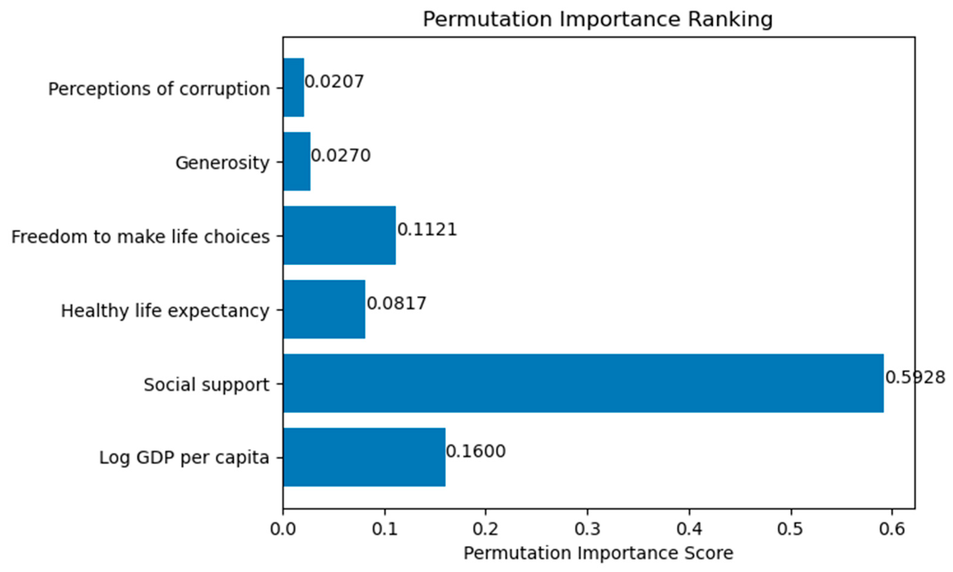
In our study, Gini significance and permutation significance analyses were conducted to determine the significance of socio-economic indicators affecting happiness. Analysis results are given in Figure 2 and Figure 3.

According to the results we obtained, the most significant factors were determined to be Social Support (Gini: 0.5592, Permutation: 0.5928), followed by Log GDP per Capita (Gini: 0.1888, Permutation: 0.1600) and Healthy Life Expectancy (Gini: 0.1034, Permutation: 0.0817). Other indicators, Freedom to Make Life Choices, Generosity, and Perceptions of Corruption, were found to be less significant factors. The analysis results revealed that the factors affecting happiness the most were Social Support and Economic Well-Being, but health-related indicators such as Healthy Life Expectancy also played an important role.

In the study, countries were divided into clusters using the K-Means clustering method on the World Happiness Index data. The K-Means algorithm is used to divide the data into $k$ predetermined clusters (in this case, 4). K-Means classifies data points according to certain centers (centroids) and assigns each data point to the closest center.

Determination of the Number of k Clusters: The Elbow method is commonly used to identify the optimal number of clusters for K-Means clustering by plotting the explained variance (or inertia) against various $k$ values [88,89,90] and identifying the “elbow” point where the rate of decrease in inertia significantly slows [91]. In our analysis, we extended this evaluation by calculating inertia for $k$ values ranging from 2 to 10. In addition, a silhouette coefficient analysis was performed, and the highest average silhouette score was observed at $k=4$, indicating that four clusters provide the best balance between intra-cluster compactness and inter-cluster separation. Therefore, by combining the insights from both the inertia and silhouette analyses, we define the optimal number of clusters as $k=4$, as illustrated in Figure 4.

Table 2. Number of clusters and cluster size.

Number of Clusters	Cluster Size
0	47
1	41
2	19
3	36

shows the number of clusters obtained as a result of the analysis and the number of members of these clusters. In our study, the quality of the clusters was evaluated using the Calinski–Harabasz Index. The Calinski–Harabasz value of 71.026 indicates that the separation between the clusters is clear and the clusters are separable from each other. This indicates that the data fit the clustering model well and the internal homogeneity of the clusters is high. However, we acknowledge that hyperparameter optimizations and different clustering algorithms should be applied to further improve this value.

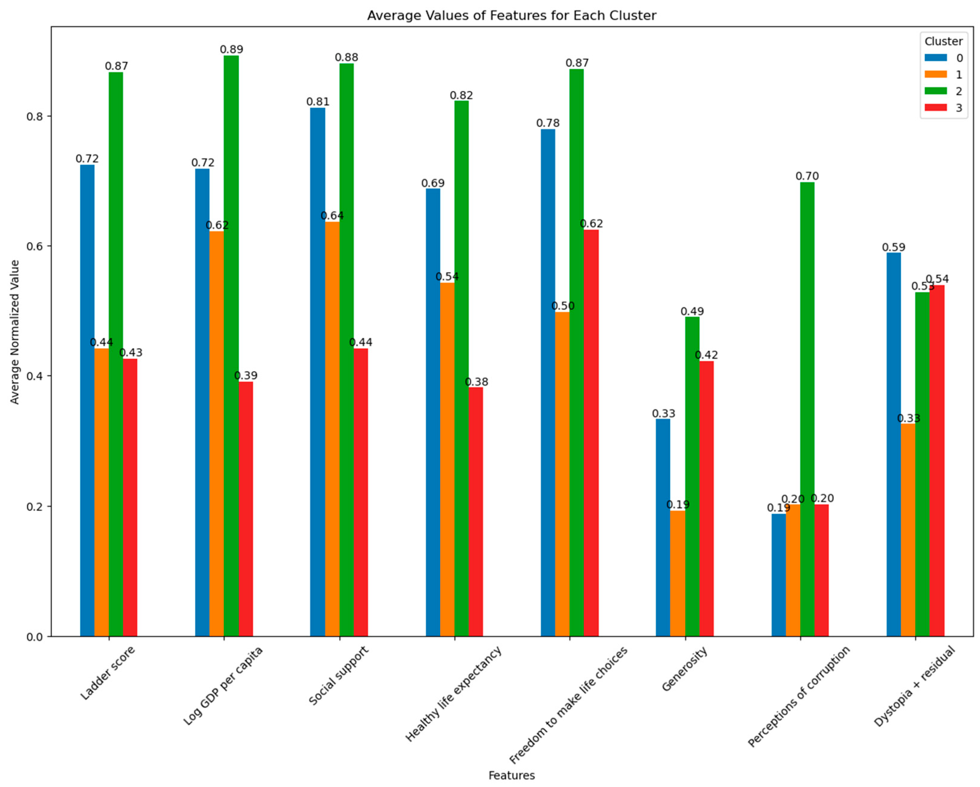
Figure 5 was created to examine the effects of factors affecting happiness levels by grouping countries in the World Happiness Index data according to similar characteristics. In this way, it was observed in which factors each cluster stood out or differed from the others, and the basic factors affecting the happiness levels of countries were made more understandable.

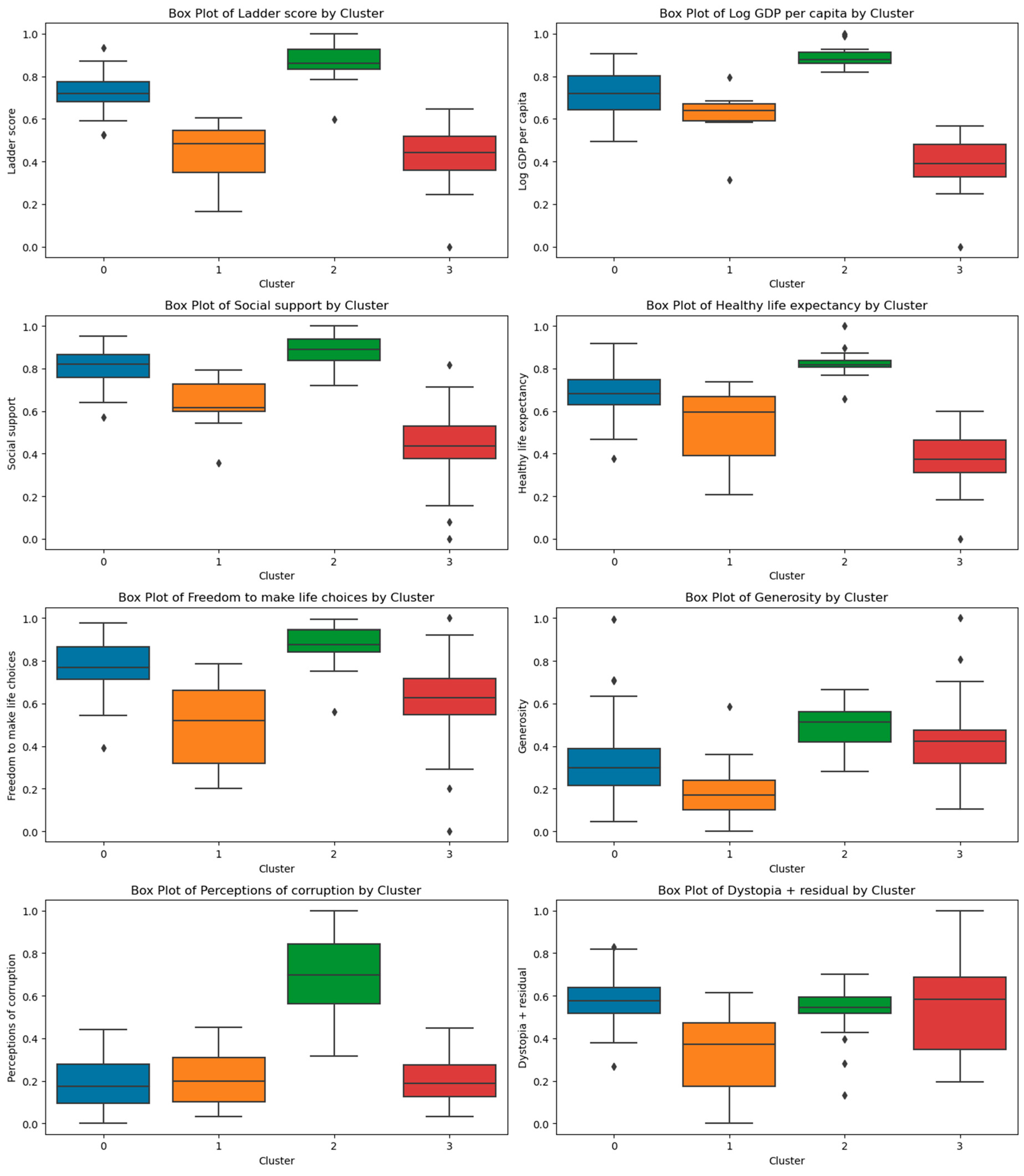
Figure 6 shows the cluster-based box plot graphs of the variables.

Table 3. Mean and standard deviation values of clusters according to variables.

Cluster	Mean
	Ladder Score	Log GDP Per Capita	Social Support	Healthy Life Expectancy	Freedom to Make Life Choices	Generosity	Perceptions of Corruption	Dystopia + Residual
0	0.724	0.718	0.812	0.687	0.779	0.333	0.187	0.589
1	0.442	0.623	0.637	0.543	0.498	0.192	0.202	0.326
2	0.867	0.893	0.880	0.822	0.871	0.490	0.698	0.528
3	0.426	0.391	0.442	0.382	0.625	0.423	0.202	0.539
Cluster	Standard Deviation
	Ladder Score	Log GDP Per Capita	Social Support	Healthy Life Expectancy	Freedom to Make Life Choices	Generosity	Perceptions of Corruption	Dystopia + Residual
0	0.079	0.100	0.083	0.101	0.120	0.178	0.115	0.112
1	0.133	0.098	0.105	0.168	0.192	0.147	0.124	0.203
2	0.085	0.050	0.076	0.061	0.095	0.104	0.184	0.132
3	0.124	0.111	0.162	0.117	0.191	0.164	0.098	0.204

shows the average values of the variables resulting from the K-Means clustering analysis.

Table 3 presents both the mean and standard deviation values of key variables as derived from the K-Means clustering analysis, grouping the countries into four clusters. The mean values help us understand the central tendencies of each group, while the standard deviations offer insight into how homogeneous or variable the countries are within each cluster.

Cluster 0: This cluster exhibits a moderate level of happiness. The relatively high means in Social Support and Economic Well-Being indicators suggest a solid socio-economic foundation. The low standard deviations for Ladder Score (0.079), Log GDP per Capita (0.100), and Social Support (0.083) indicate that the countries in Cluster 0 are homogeneous concerning these dimensions. However, the slightly higher variability in Generosity (SD = 0.178) suggests that there are moderate differences in altruistic behavior among these countries. Overall, the cluster appears stable for core economic and social measures, though some inconsistency exists in social behaviors.

Cluster 1: This cluster is characterized by a lower-than-average happiness level. Economic Well-Being and Social Support are moderate but consistently lower than those observed in Cluster 0. The standard deviations, particularly for Healthy Life Expectancy (0.168) and Freedom to Make Life Choices (0.192), are relatively high along with Dystopia + Residual (SD = 0.203)—indicating considerable variability among the countries. This suggests that while the overall means are low, the internal diversity in health and socio-economic conditions is pronounced, possibly reflecting a mix of countries with limited resources and varying degrees of Social Support.

Cluster 2: Cluster 2 represents the highest level of happiness. It has the highest mean values for Economic Well-Being, Social Support, and Health factors. The low standard deviations for Log GDP per Capita (0.050) and Healthy Life Expectancy (0.061) suggest a high degree of uniformity among the countries in terms of these core indicators. Although the mean for Perceptions of Corruption is high (0.698), indicating that corruption is perceived to be more prevalent, the moderate variability (SD = 0.184) implies that most countries in this group are consistently strong in other socio-economic areas, which may mitigate the negative impact of corruption perceptions on overall happiness.

Cluster 3: Cluster 3 shows the lowest happiness level. The low means for Economic Well-Being, Social Support, and Healthy Life Expectancy suggest significant socio-economic challenges. The higher standard deviations for Social Support (0.162) and Freedom to Make Life Choices (0.191), with the highest dispersion seen in Dystopia + Residual (SD = 0.204), reveal that there is considerable heterogeneity among the countries in this cluster. This variability indicates that while some countries may perform slightly better in certain indicators, the overall socio-economic conditions vary widely, reinforcing the characterization of Cluster 3 as facing substantial hardships.

Consequently, integrating the mean and standard deviation data provides a more nuanced picture of each cluster. Clusters with low standard deviations indicate more consistency among the countries regarding key socio-economic factors, whereas higher variability signals internal diversity. This combined analysis enhances our understanding of the factors influencing the World Happiness Index and highlights where targeted policy interventions might be most needed.

Cluster 0 displays moderate scores across economic and social variables, suggesting a balanced socio-economic profile; although these countries exhibit stable conditions, targeted improvements particularly in reducing corruption, could further enhance overall well-being. In contrast, Cluster 1 is characterized by lower-than-average scores across multiple indicators, implying significant resource constraints and highlighting the need for enhanced social services and healthcare investments to elevate living standards. Cluster 2 shows high scores in Economic Well-Being, Social Support, and Health, indicating robust socio-economic conditions; despite higher perceived corruption, the strong underlying infrastructure suggests that policies focusing on increased transparency could further elevate happiness levels. Finally, Cluster 3, with the lowest scores in key indicators, underscores substantial socio-economic challenges and emphasizes an urgent need for targeted interventions in health, education, and economic development.

The findings emphasize that Economic Well-Being, Social Support, and Health factors play a crucial role in determining happiness levels, whereas Generosity and Corruption Perceptions have a comparatively weaker influence.

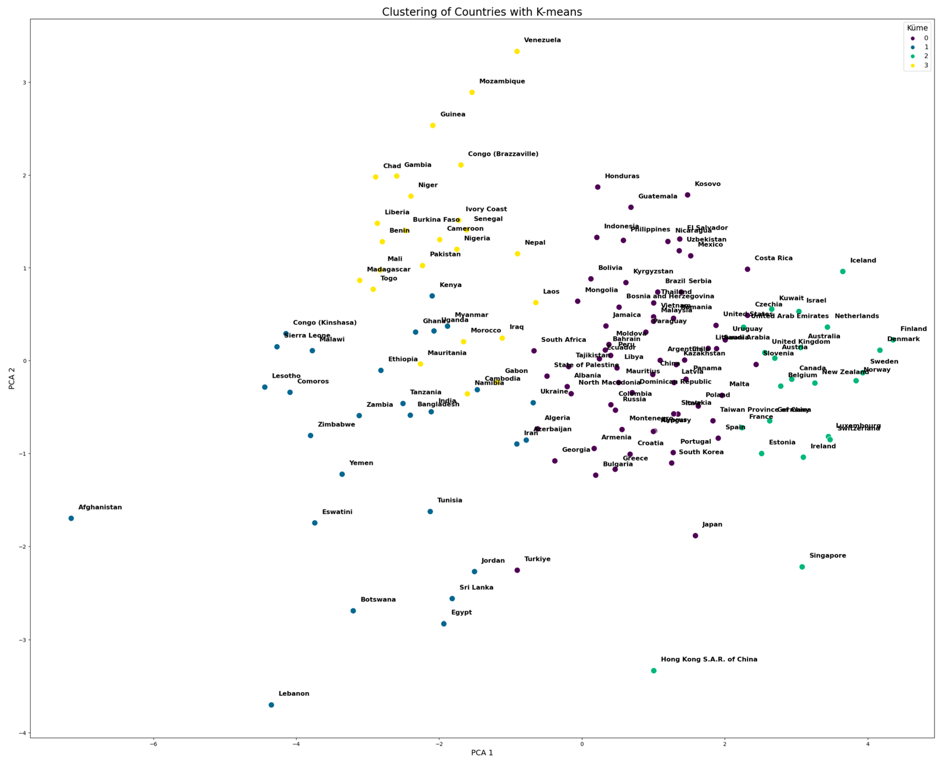
The countries in the World Happiness Index are clustered with the K-Means algorithm according to social, economic, and health indicators. The appropriate number of clusters was determined using the Elbow method and the data were reduced to two dimensions with the help of PCA. This analysis allows for determining the common factors affecting the happiness levels of countries and examining regional or economic similarities. The findings obtained provide valuable inferences on social welfare policies in different countries. The clusters in which the countries are located are shown in Figure 7.

As a result of the cluster analysis in Figure 6, countries were divided into four main clusters based on social, economic, and cultural factors. These clusters reflect the common characteristics of the countries based on factors such as happiness levels and living conditions. The results of the clustering were as follows:

Cluster 0: The nations that comprise this cluster fall largely into the categories of middle-income and developing-country status. They are mostly found in Latin America, Eastern Europe, Asia, and certainly in parts of Africa that can be found scattered across this cluster. Their combination of a social safety net, economic opportunity, and welfare provision puts them at a level of moderate happiness. The countries in this cluster may seem to cover a wide net, yet they share the common feature of confronting more economic instability and less access to desirable kinds of opportunity than the countries in the clusters that are farther to the right on this chart.

Cluster 1: This cluster primarily consists of low-income nations in Africa, some Asian countries, and countries in transition. The political instability, poverty, and poor access to health services coupled with inadequate education in these nations seriously impair their much-desired welfare standing. These nations have high-income inequality and very low levels of social security, which makes most of their citizens miserable. They have personality disorder-type problems, weak access to basic health needs, high levels of unemployment, deep poverty, and a lack of basic human necessities.

Cluster 2: Cluster 2 comprises wealthy nations that already enjoy some of the highest Social Support and living standards in the world. This group encompasses not only Northern European countries but also Australia, New Zealand, and some Gulf states. They all provide a high level of social welfare, which includes a minimum level of economic security; universal, or nearly universal, access to good health services and educational opportunities; and lasting political stability. These same nations, with their high living standards, are generally at the top of happiness surveys.

Cluster 3: Countries in Cluster 3 are primarily low-income, high-poverty countries, with some located in Africa and South Asia. These countries are beset by political conflict, high rates of unemployment, and inadequate access to health and educational services. The unstable economic conditions of these countries may also directly impact their residents’ levels of happiness. Most of the countries in this cluster seem to be experiencing civil strife or seriously troubling economic situations, which translate into seriously troubling welfare levels for the residents of those countries.

As a result, it shows that geographical and economic factors have a decisive effect on happiness. While Northern European and some Western countries are in the group with high Social Support and Economic Well-Being, African and some South Asian countries have lower happiness levels due to problems such as poverty and political instability. These findings emphasize the necessity of regional development policies aimed at increasing happiness in developing or underdeveloped countries while maintaining the welfare levels of developed countries.

These effects of regional differences on happiness can be considered an important guide in the social policy development process.

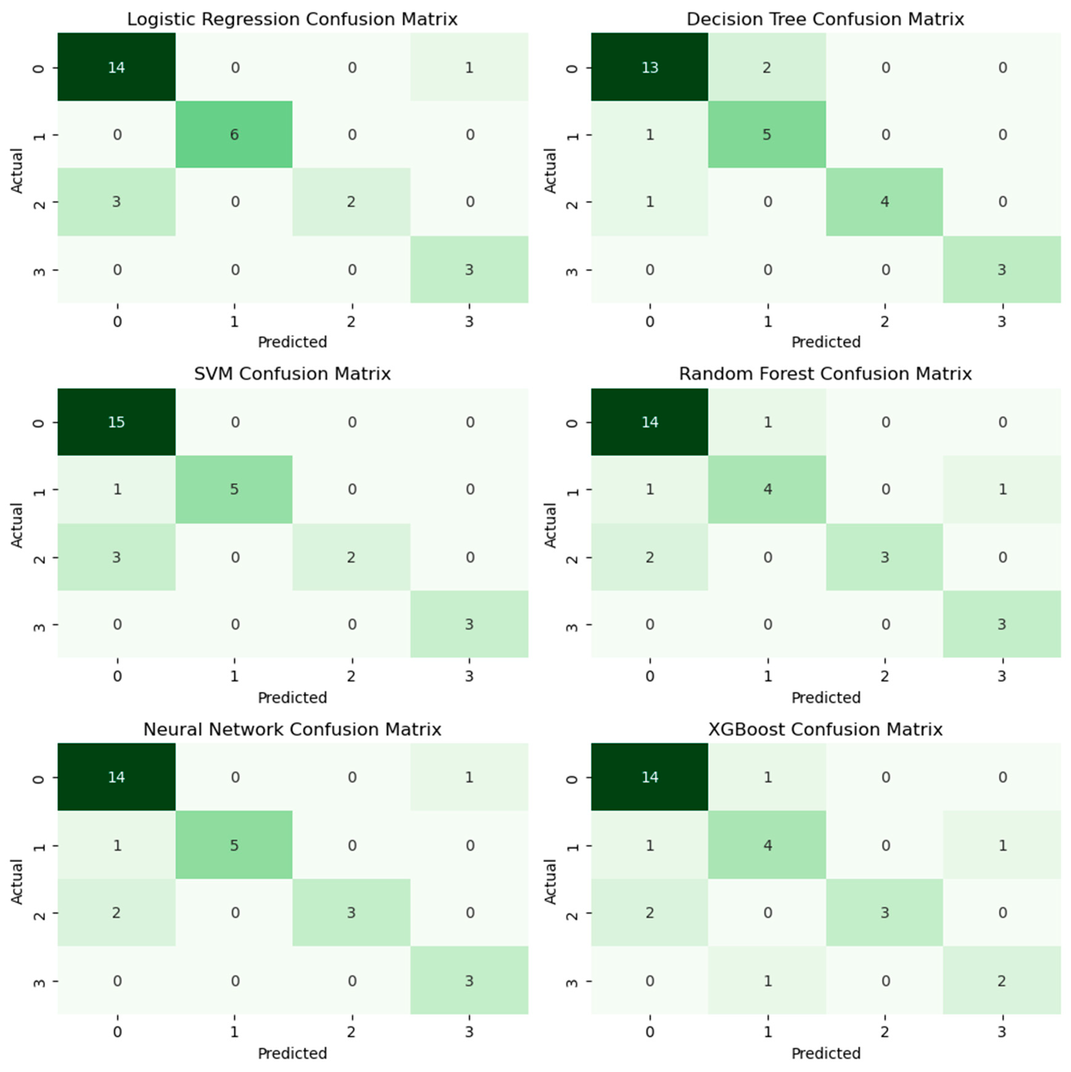
To indirectly validate the separability and robustness of the clusters derived from the K-Means analysis, various classification algorithms were employed to predict cluster membership based on the original features. Confusion matrix results of the classification algorithms used are given in Figure 8.

The accuracy values of the algorithms used to test the accuracy of cluster analysis in the study are given in

Table 4. Logistic Regression accuracy.

Logistic Regression Accuracy: 0.8620689655172413
Logistic Regression Classification Report:
	precision	recall	f1-score	Support
Cluster
0	0.82	0.93	0.87	15
1	1.00	1.00	1.00	6
2	1.00	0.40	0.57	5
3	0.75	1.00	0.86	3
accuracy			0.86	29
macro avg	0.89	0.83	0.83	29
weighted avg	0.88	0.86	0.85	29

,

Table 5. Decision Tree accuracy.

Decision Tree Accuracy: 0.8620689655172413
Decision Tree Classification Report:
	precision	recall	f1-score	Support
Cluster
0	0.87	0.87	0.87	15
1	0.71	0.83	0.77	6
2	1.00	0.80	0.89	5
3	1.00	1.00	1.00	3
accuracy			0.86	29
macro avg	0.90	0.88	0.88	29
weighted avg	0.87	0.86	0.86	29

,

Table 6. SVM accuracy.

SVM Accuracy: 0.8620689655172413
SVM Classification Report:
	precision	recall	f1-score	Support
Cluster
0	0.79	1.00	0.88	15
1	1.00	0.83	0.91	6
2	1.00	0.40	0.57	5
3	1.00	1.00	1.00	3
accuracy			0.86	29
macro avg	0.95	0.81	0.84	29
weighted avg	0.89	0.86	0.85	29

,

Table 7. Random Forest accuracy.

Random Forest Accuracy: 0.8275862068965517
Random Forest Accuracy: 0.8275862068965517
	precision	recall	f1-score	support
Cluster
0	0.82	0.93	0.87	15
1	0.80	0.67	0.73	6
2	1.00	0.60	0.75	5
3	0.75	1.00	0.86	3
accuracy			0.83	29
macro avg	0.84	0.80	0.80	29
weighted avg	0.84	0.83	0.82	29

,

Table 8. Neural Network accuracy.

Neural Network Accuracy: 0.8620689655172413
Neural Network Classification Report:
	precision	recall	f1-score	support
Cluster
0	0.82	0.93	0.87	15
1	1.00	0.83	0.91	6
2	1.00	0.60	0.75	5
3	0.75	1.00	0.86	3
accuracy			0.86	29
macro avg	0.89	0.84	0.85	29
weighted avg	0.88	0.86	0.86	29

and

Table 9. XGBoost accuracy.

XGBoost Accuracy: 0.7931034482758621
XGBoost Classification Report:
	precision	recall	f1-score	support
Cluster
0	0.82	0.93	0.87	15
1	0.67	0.67	0.67	6
2	1.00	0.60	0.75	5
3	0.67	0.67	0.67	3
accuracy			0.79	29
macro avg	0.79	0.72	0.74	29
weighted avg	0.81	0.79	0.79	29

.

The Logistic Regression model achieved an overall accuracy of 86.2%. It performed exceptionally well in Class 0 and Class 1, with recall values of 93% and 100%, respectively. However, its performance in Class 2 was weak, with a recall of only 40%, indicating that the model frequently misclassified instances of this class. This suggests that Class 2 shares characteristics with other classes, leading to a high misclassification rate. Class 3 was well classified, achieving 100% recall, which means no instances of this class were misclassified.

The Decision Tree model also achieved an accuracy of 86.2%, but it outperformed Logistic Regression in identifying Class 2 with a recall of 80% (double that of Logistic Regression). This improvement indicates that Decision Trees might be better at distinguishing nonlinear patterns in the dataset for Class 2. The model also achieved 100% recall in Class 3, showing strong performance in this class. However, it exhibited slightly lower recall in Class 1 (83%), meaning some instances of this class were misclassified.

The SVM model performed similarly, also reaching an accuracy of 86.2%. It excelled in Class 0 and Class 3, achieving 100% recall in both classes. However, similar to Logistic Regression, it struggled with Class 2, with a recall of only 40%. This indicates that SVM may not effectively separate Class 2 from other classes due to its feature distribution. Despite its strong performance in most classes, the low recall for Class 2 suggests that further feature engineering or hyperparameter tuning could improve its classification ability.

The degree of accuracy shown by the Random Forest model was found to be relatively less than that of previous models at 82.8%. The model retained high recall at 93% in Class 0, but its performance fell short for Class 1 and Class 2, giving 67% and 60% recall scores, respectively. Thus, Random Forest seems to struggle in distinguishing some minority classes, possibly because of an imbalance in the dataset or sensitivity to noise present in the smaller classes.

The Artificial Neural Network model also attained an accuracy of 86.2%, the same as those of the prior models. It performed strongly for both Classes 0 and 1, but Class 2 had a recall value of 60%, which was better than the scores of SVM and Logistic Regression but poorer than that of Decision Trees. This indicates that while the Neural Network can learn complex patterns, it probably needs to be fed data either in larger quantities or with better optimization techniques to improve recall on harder to classify classes.

Lastly, the XGBoost model had the lowest accuracy at 79.3%, with significant weaknesses in Class 1 and Class 3 (both with 67% recall). Its recall in Class 2 was also only 60%, which is better than some models but still suboptimal. The lower overall accuracy suggests that XGBoost may not be the best choice for this clustering task, as it struggles to maintain high recall across multiple classes.

In conclusion, while most models performed well in certain classes, Class 2 posed a significant challenge, with most models misclassifying a large portion of its instances. Future improvements could focus on feature engineering, class balancing techniques, and hyperparameter tuning to improve classification in Class 2.

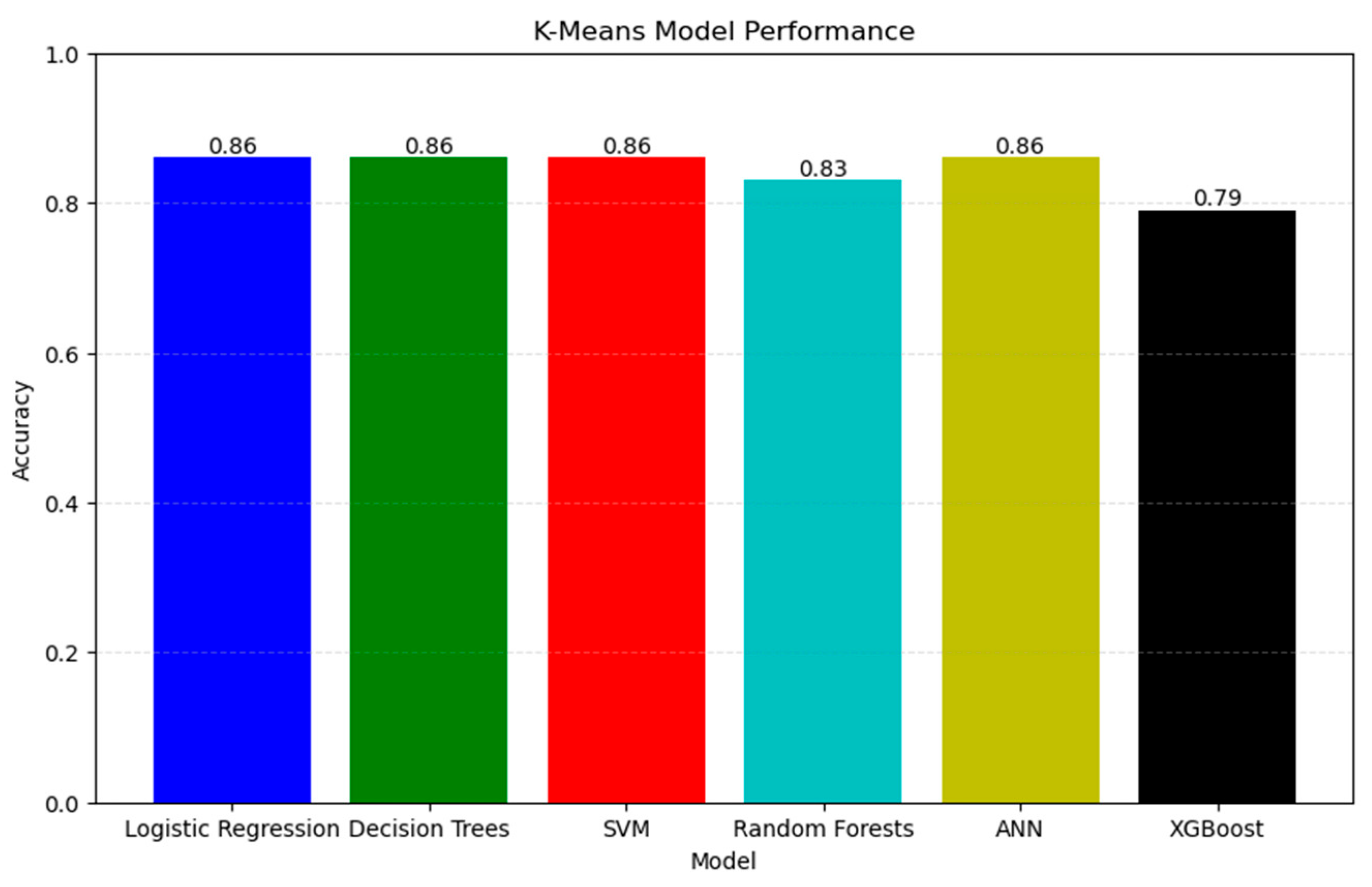
Figure 9 compares the performance success of the algorithms used to test the accuracy of cluster analysis.

The accuracy values obtained in this study were compared with previous research using similar methods. Akanbi et al. [18] conducted a study predicting the happiness index using machine learning models such as XGBoost and Random Forest. Their results showed that XGBoost achieved an R-squared value of 85.03%, while Random Forest obtained 83.68%. Although their study focused on regression-based predictions rather than classification, our findings suggest that XGBoost’s lower classification accuracy (79.3%) may be influenced by differences in task complexity and dataset characteristics. Furthermore, Jannani, Sael and Benabbou [3] utilized regression models, including Random Forest and XGBoost, for happiness prediction and reported that Random Forest achieved the highest performance with an R² score of 0.93667, while XGBoost performed comparably but slightly lower. These findings support our observation that Random Forest and XGBoost behave differently depending on whether the task is classification or regression. The results of our study align with these findings, confirming that Random Forest generally performs well in happiness prediction tasks, while XGBoost shows strong predictive power in regression but comparatively lower accuracy in classification tasks. These comparisons confirm that our results are consistent with existing literature and represent a meaningful benchmark in the analysis of happiness classification models.

6. Conclusions and Discussion

The presented study aimed to compare the accuracy of several machine learning algorithms (Logistic Regression, Decision Tree, SVM, Random Forest, ANN, and XGBoost) using data from the World Happiness Index. In the analysis, Logistic Regression, Decision Tree, SVM, and Neural Network emerged as the top four algorithms for accuracy achieving a very respectable 86.2% performance rate, while XGBoost lagged with just 79.3%. When classified through K-Means clustering, the data were divided into four main groups corresponding to distinct happiness levels defined by socio-economic factors.

While the manuscript reports detailed accuracy metrics, it is important to note that these metrics serve only as a validation tool for our clustering analysis. The primary focus of our study was to investigate the underlying socioeconomic determinants of national happiness. The study results provide a strong foundation for efficient classification and analysis using ML algorithms, particularly when dealing with complex, multidimensional datasets. Moreover, the comparisons indicate that the performance of different algorithms can vary under diverse conditions and that some methods may excel when applied to specific aspects of the data.

From a practical perspective, our clustering analysis reveals that key factors such as Economic Performance, Social Support, and Health have a pronounced influence on national happiness. Based on these findings, we recommend that policymakers prioritize initiatives aimed at enhancing economic stability—through targeted fiscal policies and investments—as well as improving public healthcare infrastructure to boost overall well-being. Additionally, strengthening Social Support networks by investing in community-based programs and social safety measures, along with implementing anti-corruption measures, can further contribute to increasing national happiness levels.

Future work will focus on further refining these models through advanced feature engineering, hyperparameter optimization, and the exploration of ensemble approaches to improve the classification of challenging classes. In addition, we plan to extend our analysis by incorporating temporal dynamics and additional socioeconomic variables to assess changes in national happiness over time. This extended analysis will not only improve the technical robustness of our methodology but also expand the practical implications of our findings, ultimately guiding targeted policy interventions.

From a practical perspective, the insights derived from our clustering analysis can directly inform policymakers by highlighting the key socioeconomic factors that drive national happiness. These findings can be used to develop targeted interventions aimed at improving economic stability, enhancing Social Support networks, and expanding access to quality healthcare, thereby ultimately contributing to improved well-being on a national scale.

Consequently, this study underscores the need for a reevaluation of social and economic policies aimed at increasing happiness levels. It represents a milestone in creating strategies to boost happiness in developing countries and is recommended as a blueprint for further research on model selection and the practical application of ML algorithms. The study’s results also offer valuable guidance for the design and implementation of social welfare policies.

References

1. Lakócai, C. How Sustainable Is Happiness? An Enquiry about the Sustainability and Wellbeing Performance of Societies. Int. J. Sustain. Dev. World Ecol. 2023, 30, 420–427. [Google Scholar] [CrossRef]
2. Glatzer, W. Worldwide Indicators for Quality of Life: The Ten Leading Countries in the View of the Peoples and the Measurements of Experts around 2020. SCIREA J. Sociol. 2023, 7, 368–383. [Google Scholar] [CrossRef]
3. Jannani, A.; Sael, N.; Benabbou, F. Machine Learning for the Analysis of Quality of Life Using the World Happiness Index and Human Development Indicators. Math. Model. Comput. 2023, 10, 534–546. [Google Scholar] [CrossRef]
4. Du, L.; Liang, Y.; Ahmad, M.I.; Zhou, P. K-Means Clustering Based on Chebyshev Polynomial Graph Filtering. In Proceedings of the ICASSP 2024—2024 IEEE International Conference on Acoustics, Speech and Signal Processing (ICASSP), Seoul, Republic of Korea, 14–19 April 2024; IEEE: New York, NY, USA, 2024; pp. 7175–7179. [Google Scholar]
5. Spowart, S. A Path to Happiness. In Happiness and Wellness—Biopsychosocial and Anthropological Perspectives; IntechOpen: London, UK, 2023. [Google Scholar]
6. Lomas, T. Happiness; The MIT Press: Cambridge, MA, USA, 2023; ISBN 9780262370837. [Google Scholar]
7. Ağralı Ermiş, S.; Dereceli, E. The Effect of the Life Satisfaction of Individuals Over 65 Years on Their Happiness. Turk. J. Sport Exerc. 2023, 25, 310–318. [Google Scholar] [CrossRef]
8. Tipi, R.; Şahin, H.; Doğru, Ş.; Zengin Bintaş, G.Ç. A Comparative Evalution on the Prediction Performance of Regression Algorithms in Machine Learning for Die Design Cost Estimation. Electron. Lett. Sci. Eng. 2023, 19, 48–62. [Google Scholar]
9. Dünder, M.; Dünder, E. Comparison of Machine Learning Algorithms in the Presence of Class Imbalance in Categorical Data: An Application on Student Success. J. Digit. Technol. Educ. 2024, 3, 28–38. [Google Scholar]
10. Dixit, S.; Chaudhary, M.; Sahni, N. Network Learning Approaches to Study World Happiness. arXiv 2020, arXiv:2007.09181. [Google Scholar]
11. Chen, S.; Yang, M.; Lin, Y. Predicting Happiness Levels of European Immigrants and Natives: An Application of Artificial Neural Network and Ordinal Logistic Regression. Front. Psychol. 2022, 13, 1012796. [Google Scholar] [CrossRef]
12. Khder, M.; Sayf, M.; Fujo, S. Analysis of World Happiness Report Dataset Using Machine Learning Approaches. Int. J. Adv. Soft Comput. Its Appl. 2022, 14, 15–34. [Google Scholar] [CrossRef]
13. Zhang, Y. Analyze and Predict the 2022 World Happiness Report Based on the Past Year’s Dataset. J. Comput. Sci. 2023, 19, 483–492. [Google Scholar] [CrossRef]
14. Timmapuram, M.; Ramdas, R.; Vutkur, S.R.; Mali, Y.R.; Vasanth, K. Understanding the Regional Differences in World Happiness Index Using Machine Learning. In Proceedings of the 2023 International Conference on Innovative Computing, Intelligent Communication and Smart Electrical Systems (ICSES), Chennai, India, 14–15 December 2023; IEEE: New York, NY, USA, 2023; pp. 1–9. [Google Scholar]
15. Liu, A.; Zhang, Y. Happiness Index Prediction Using Machine Learning Algorithms. Appl. Comput. Eng. 2023, 5, 386–389. [Google Scholar] [CrossRef]
16. Sihombing, P.R.; Budiantono, S.; Arsani, A.M.; Aritonang, T.M.; Kurniawan, M.A. Comparison of Regression Analysis with Machine Learning Supervised Predictive Model Techniques. J. Ekon. Dan Stat. Indones. 2023, 3, 113–118. [Google Scholar] [CrossRef]
17. Akanbi, K.; Jones, Y.; Oluwadare, S.; Nti, I.K. Predicting Happiness Index Using Machine Learning. In Proceedings of the 2024 IEEE 3rd International Conference on Computing and Machine Intelligence (ICMI), Mt Pleasant, MI, USA, 13–14 April 2024; IEEE: New York, NY, USA, 2024; pp. 1–5. [Google Scholar]
18. Jaiswal, R.; Gupta, S. Money Talks, Happiness Walks: Dissecting the Secrets of Global Bliss with Machine Learning. J. Chin. Econ. Bus. Stud. 2024, 22, 111–158. [Google Scholar] [CrossRef]
19. Airlangga, G.; Liu, A. A Hybrid Gradient Boosting and Neural Network Model for Predicting Urban Happiness: Integrating Ensemble Learning with Deep Representation for Enhanced Accuracy. Mach. Learn. Knowl. Extr. 2025, 7, 4. [Google Scholar] [CrossRef]
20. Rusdiana, L.; Hardita, V.C. Algoritma K-Means Dalam Pengelompokan Surat Keluar Pada Program Studi Teknik Informatika STMIK Palangkaraya. J. Saıntekom 2023, 13, 55–66. [Google Scholar] [CrossRef]
21. Paratama, M.A.Y.; Hidayah, A.R.; Avini, T. Clusterıng K-Means Untuk Analısıs Pola Persebaran Bencana Alam Dı Indonesıa. J. Inform. Dan Tekonologi Komput. (JITEK) 2023, 3, 108–114. [Google Scholar] [CrossRef]
22. Cui, J.; Liu, J.; Liao, Z. Research on K-Means Clustering Algorithm and Its Implementation. In Proceedings of the 2nd International Conference on Computer Science and Electronics Engineering (ICCSEE 2013), Hangzhou, China, 22–23 March 2013; Atlantis Press: Paris, France, 2013. [Google Scholar]
23. Wu, B. K-Means Clustering Algorithm and Python Implementation. In Proceedings of the 2021 IEEE International Conference on Computer Science, Artificial Intelligence and Electronic Engineering (CSAIEE), Virtual Conference, 20–22 August 2021; IEEE: New York, NY, USA, 2021; pp. 55–59. [Google Scholar]
24. Zhao, Y.; Zhou, X. K-Means Clustering Algorithm and Its Improvement Research. J. Phys. Conf. Ser. 2021, 1873, 012074. [Google Scholar] [CrossRef]
25. Kamgar-Parsi, B.; Kamgar-Parsi, B. Penalized K-Means Algorithms for Finding the Number of Clusters. In Proceedings of the 2020 25th International Conference on Pattern Recognition (ICPR), Milan, Italy, 10–15 January 2021; IEEE: New York, NY, USA, 2021; pp. 969–974. [Google Scholar]
26. Sirikayon, C.; Thammano, A. Deterministic Initialization of K-Means Clustering by Data Distribution Guide. In Proceedings of the 2022 Joint International Conference on Digital Arts, Media and Technology with ECTI Northern Section Conference on Electrical, Electronics, Computer and Telecommunications Engineering (ECTI DAMT & NCON), Chiang Rai, Thailand, 26–28 January 2022; IEEE: New York, NY, USA, 2022; pp. 279–284. [Google Scholar]
27. Thulasidas, M. A Quality Metric for K-Means Clustering. In Proceedings of the 2018 14th International Conference on Natural Computation, Fuzzy Systems and Knowledge Discovery (ICNC-FSKD), Huangshan, China, 28–30 July 2018; IEEE: New York, NY, USA, 2018; pp. 752–757. [Google Scholar]
28. Dong, Q.; Chen, X.; Huang, B. Logistic Regression. Data Anal. Pavement Eng. 2024, 141–152. [Google Scholar] [CrossRef]
29. Kravets, P.; Pasichnyk, V.; Prodaniuk, M. Mathematical Model of Logistic Regression for Binary Classification. Part 1. Regression Models of Data Generalization. Vìsnik Nacìonalʹnogo unìversitetu “Lʹvìvsʹka polìtehnìka”. Serìâ Ìnformacìjnì sistemi ta merežì 2024, 15, 290–321. [Google Scholar] [CrossRef]
30. Ma, Q. Recent Applications and Perspectives of Logistic Regression Modelling in Healthcare. Theor. Nat. Sci. 2024, 36, 185–190. [Google Scholar] [CrossRef]
31. Zaidi, A.; Al Luhayb, A.S.M. Two Statistical Approaches to Justify the Use of the Logistic Function in Binary Logistic Regression. Math. Probl. Eng. 2023, 2023, 5525675. [Google Scholar] [CrossRef]
32. Zaidi, A. Mathematical Justification on the Origin of the Sigmoid in Logistic Regression. Cent. Eur. Manag. J. 2022, 30, 1327–1337. [Google Scholar] [CrossRef]
33. Kawano, S.; Konishi, S. Nonlinear Logistic Discrimination via Regularized Gaussian Basis Expansions. Commun. Stat. Simul. Comput. 2009, 38, 1414–1425. [Google Scholar] [CrossRef]
34. Thierry, D. Logistic Regression, Neural Networks and Dempster–Shafer Theory: A New Perspective. Knowl. Based Syst. 2019, 176, 54–67. [Google Scholar] [CrossRef]
35. Yuen, J.; Twengström, E.; Sigvald, R. Calibration and Verification of Risk Algorithms Using Logistic Regression. Eur. J. Plant Pathol. 1996, 102, 847–854. [Google Scholar] [CrossRef]
36. Bokov, A.; Antonenko, S. Application of Logistic Regression Equation Analysis Using Derivatives for Optimal Cutoff Discriminative Criterion Estimation. Ann. Math. Phys. 2020, 3, 032–035. [Google Scholar] [CrossRef]
37. Grace, A.L.; Thenmozhi, M. Optimizing Logistics with Regularization Techniques: A Comparative Study. In Proceedings of the 2023 IEEE World Conference on Applied Intelligence and Computing (AIC), Sonbhadra, India, 29–30 July 2023; IEEE: New York, NY, USA, 2023; pp. 338–344. [Google Scholar]
38. Reznychenko, T.; Uglickich, E.; Nagy, I. Accuracy Comparison of Logistic Regression, Random Forest, and Neural Networks Applied to Real MaaS Data. In Proceedings of the 2024 Smart City Symposium Prague (SCSP), Prague, Czech Republic, 23–24 May 2024; IEEE: New York, NY, USA, 2024; pp. 1–5. [Google Scholar]
39. Xu, C.; Peng, Z.; Jing, W. Sparse Kernel Logistic Regression Based on L 1/2 Regularization. Sci. China Inf. Sci. 2013, 56, 1–16. [Google Scholar] [CrossRef]
40. Huang, H.-H.; Liu, X.-Y.; Liang, Y. Feature Selection and Cancer Classification via Sparse Logistic Regression with the Hybrid L1/2 +2 Regularization. PLoS ONE 2016, 11, e0149675. [Google Scholar] [CrossRef]
41. Hsieh, W.W. Decision Trees, Random Forests and Boosting. In Introduction to Environmental Data Science; Cambridge University Press: Cambridge, UK, 2023; pp. 473–493. [Google Scholar]
42. Chopra, D.; Khurana, R. Decision Trees. In Introduction to Machine Learning with Python; Bentham Science Publishers: Sharjah, United Arab Emirates, 2023; pp. 74–82. [Google Scholar]
43. Lai, Y. Research on the Application of Decision Tree in Mobile Marketing. In Frontier Computing; Springer: Singapore, 2023; pp. 1488–1495. [Google Scholar]
44. Zhao, X.; Nie, X. Splitting Choice and Computational Complexity Analysis of Decision Trees. Entropy 2021, 23, 1241. [Google Scholar] [CrossRef]
45. Tangirala, S. Evaluating the Impact of GINI Index and Information Gain on Classification Using Decision Tree Classifier Algorithm. Int. J. Adv. Comput. Sci. Appl. 2020, 11, 612–619. [Google Scholar] [CrossRef]
46. Sharma, N.; Iqbal, S.I.M. Applying Decision Tree Algorithm Classification and Regression Tree (CART) Algorithm to Gini Techniques Binary Splits. Int. J. Eng. Adv. Technol. 2023, 12, 77–81. [Google Scholar] [CrossRef]
47. Aaboub, F.; Chamlal, H.; Ouaderhman, T. Statistical Analysis of Various Splitting Criteria for Decision Trees. J. Algorithm. Comput. Technol. 2023, 17, 1–13. [Google Scholar] [CrossRef]
48. Pathan, S.; Sharma, S.K. Design an Optimal Decision Tree Based Algorithm to Improve Model Prediction Performance. Int. J. Recent Innov. Trends Comput. Commun. 2023, 11, 127–133. [Google Scholar] [CrossRef]
49. Disha, R.A.; Waheed, S. Performance Analysis of Machine Learning Models for Intrusion Detection System Using Gini Impurity-Based Weighted Random Forest (GIWRF) Feature Selection Technique. Cybersecurity 2022, 5, 1. [Google Scholar] [CrossRef]
50. Chandra, B.; Paul Varghese, P. Fuzzifying Gini Index Based Decision Trees. Expert Syst. Appl. 2009, 36, 8549–8559. [Google Scholar] [CrossRef]
51. Zeng, G. On Impurity Functions in Decision Trees. Commun. Stat. Theory Methods 2025, 54, 701–719. [Google Scholar] [CrossRef]
52. Khanduja, D.K.; Kaur, S. The Categorization of Documents Using Support Vector Machines. Int. J. Sci. Res. Comput. Sci. Eng. 2023, 11, 1–12. [Google Scholar] [CrossRef]
53. Ramadani, K.; Erda, G.E.G. World Greenhouse Gas Emission Classification Using Support Vector Machine (SVM) Method. Parameter J. Stat. 2024, 4, 1–8. [Google Scholar] [CrossRef]
54. Ananda, J.S.; Fendriani, Y.; Pebralia, J. Classification Analysis Of Brain Tumor Dissease In Radiographic Images Using Support Vector Machines (SVM) With Python. J. Online Phys. 2024, 9, 110–115. [Google Scholar] [CrossRef]
55. Wang, Q. Support Vector Machine Algorithm in Machine Learning. In Proceedings of the 2022 IEEE International Conference on Artificial Intelligence and Computer Applications (ICAICA), Dalian, China, 24–26 June 2022; IEEE: New York, NY, USA, 2022; pp. 750–756. [Google Scholar]
56. Dabas, A. Application of Support Vector Machines in Machine Learning. 2024. Available online: https://d197for5662m48.cloudfront.net/documents/publicationstatus/216532/preprint_pdf/0712c8e4f08648a45d2de5c43f47e9e6.pdf (accessed on 10 February 2025).
57. Li, H. Support Vector Machine. In Machine Learning Methods; Springer Nature: Singapore, 2024; pp. 127–177. [Google Scholar]
58. Huang, C.; Zhang, R.; Zhang, J.; Guo, X.; Wei, P.; Wang, L.; Huang, P.; Li, W.; Wang, Y. A Novel Method for Fatigue Design of FRP-Strengthened RC Beams Based on Machine Learning. Compos. Struct. 2025, 359, 118867. [Google Scholar] [CrossRef]
59. Tarigan, A.; Agushinta, D.; Suhendra, A.; Budiman, F. Determination of SVM-RBF Kernel Space Parameter to Optimize Accuracy Value of Indonesian Batik Images Classification. J. Comput. Sci. 2017, 13, 590–599. [Google Scholar] [CrossRef]
60. Wainer, J.; Fonseca, P. How to Tune the RBF SVM Hyperparameters? An Empirical Evaluation of 18 Search Algorithms. Artif. Intell. Rev. 2021, 54, 4771–4797. [Google Scholar] [CrossRef]
61. Aiman Ngadilan, M.A.; Ismail, N.; Rahiman, M.H.F.; Taib, M.N.; Mohd Ali, N.A.; Tajuddin, S.N. Radial Basis Function (RBF) Tuned Kernel Parameter of Agarwood Oil Compound for Quality Classification Using Support Vector Machine (SVM). In Proceedings of the 2018 9th IEEE Control and System Graduate Research Colloquium (ICSGRC), Shah Alam, Malaysia, 3–4 August 2018; IEEE: New York, NY, USA, 2018; pp. 64–68. [Google Scholar]
62. Maindola, M.; Al-Fatlawy, R.R.; Kumar, R.; Boob, N.S.; Sreeja, S.P.; Sirisha, N.; Srivastava, A. Utilizing Random Forests for High-Accuracy Classification in Medical Diagnostics. In Proceedings of the 2024 7th International Conference on Contemporary Computing and Informatics (IC3I), Greater Noida, India, 18–20 September 2024; IEEE: New York, NY, USA, 2024; pp. 1679–1685. [Google Scholar]
63. Zhu, J.; Zhang, A.; Zheng, H. Research on Predictive Model Based on Ensemble Learning. Highlights Sci. Eng. Technol. 2023, 57, 311–319. [Google Scholar] [CrossRef]
64. Gu, Q.; Tian, J.; Li, X.; Jiang, S. A Novel Random Forest Integrated Model for Imbalanced Data Classification Problem. Knowl. Based Syst. 2022, 250, 109050. [Google Scholar] [CrossRef]
65. Ignatenko, V.; Surkov, A.; Koltcov, S. Random Forests with Parametric Entropy-Based Information Gains for Classification and Regression Problems. PeerJ Comput. Sci. 2024, 10, e1775. [Google Scholar] [CrossRef]
66. Salman, H.A.; Kalakech, A.; Steiti, A. Random Forest Algorithm Overview. Babylon. J. Mach. Learn. 2024, 2024, 69–79. [Google Scholar] [CrossRef] [PubMed]
67. Tarchoune, I.; Djebbar, A.; Merouani, H.F. Improving Random Forest with Pre-Pruning Technique for Binary Classification. All Sci. Abstr. 2023, 1, 11. [Google Scholar] [CrossRef]
68. Ren, Y.; Zhu, X.; Bai, K.; Zhang, R. A New Random Forest Ensemble of Intuitionistic Fuzzy Decision Trees. IEEE Trans. Fuzzy Syst. 2023, 31, 1729–1741. [Google Scholar] [CrossRef]
69. Aryan Rose, A.R. How Do Artificial Neural Networks Work. J. Adv. Sci. Technol. 2024, 20, 172–177. [Google Scholar] [CrossRef]
70. Hussain, N.Y. Deep Learning Architectures Enabling Sophisticated Feature Extraction and Representation for Complex Data Analysis. Int. J. Innov. Sci. Res. Technol. (IJISRT) 2024, 9, 2290–2300. [Google Scholar] [CrossRef]
71. Kalita, J.K.; Bhattacharyya, D.K.; Roy, S. Artificial Neural Networks. In Fundamentals of Data Science; Elsevier: Amsterdam, The Netherlands, 2024; pp. 121–160. [Google Scholar]
72. Piña, O.C.; Villegas-Jimenéz, A.A.; Aguilar-Canto, F.; Gambino, O.J.; Calvo, H. Neuroscience-Informed Interpretability of Intermediate Layers in Artificial Neural Networks. In Proceedings of the 2024 International Joint Conference on Neural Networks (IJCNN), Yokohama, Japan, 30 June–5 July 2024; IEEE: New York, NY, USA, 2024; pp. 1–8. [Google Scholar]
73. Wang, L.; Fu, K. Artificial Neural Networks. In Wiley Encyclopedia of Computer Science and Engineering; Wiley: Hoboken, NJ, USA, 2009; pp. 181–188. [Google Scholar]
74. Schonlau, M. Neural Networks; Springer Nature: Singapore, 2023; pp. 285–322. [Google Scholar]
75. Dutta, S.; Adhikary, S. Evolutionary Swarming Particles To Speedup Neural Network Parametric Weights Updates. In Proceedings of the 2023 9th International Conference on Smart Computing and Communications (ICSCC), Kochi, Kerala, India, 17–19 August 2023; IEEE: New York, NY, USA, 2023; pp. 413–418. [Google Scholar]
76. Yang, L. Theoretical Analysis of Adam Optimizer in the Presence of Gradient Skewness. Int. J. Appl. Sci. 2024, 7, 27. [Google Scholar] [CrossRef]
77. Lei, X.; Liu, J.; Ye, X. Research on Network Traffic Anomaly Detection Technology Based on XGBoost. In Proceedings of the International Conference on Algorithms, High Performance Computing, and Artificial Intelligence (AHPCAI 2024), Zhengzhou, China, 21–23 June 2024; Loskot, P., Hu, L., Eds.; SPIE: Bellingham, WA, USA, 2024; p. 69. [Google Scholar]
78. Pang, Y.; Wang, X.; Tang, Y.; Gu, G.; Chen, J.; Yang, B.; Ning, L.; Bao, C.; Zhou, S.; Cao, X.; et al. A Traffic Accident Early Warning Model Based on XGBOOST. In Proceedings of the Fourth International Conference on Advanced Algorithms and Neural Networks (AANN 2024), Qingdao, China, 9–11 August 2024; Lu, Q., Zhang, W., Eds.; SPIE: Bellingham, WA, USA, 2024; p. 120. [Google Scholar]
79. Rani, R.; Gill, K.S.; Upadhyay, D.; Devliyal, S. XGBoost-Driven Insights: Enhancing Chronic Kidney Disease Detection. In Proceedings of the 2024 5th International Conference on Smart Electronics and Communication (ICOSEC), Trichy, India, 18–20 September 2024; IEEE: New York, NY, USA, 2024; pp. 1131–1134. [Google Scholar]
80. Murdiansyah, D.T. Prediksi Stroke Menggunakan Extreme Gradient Boosting. J. Inform. Dan Komput. JIKO 2024, 8, 419. [Google Scholar] [CrossRef]
81. Chimphlee, W.; Chimphlee, S. Hyperparameters Optimization XGBoost for Network Intrusion Detection Using CSE-CIC-IDS 2018 Dataset. IAES Int. J. Artif. Intell. IJ-AI 2024, 13, 817. [Google Scholar] [CrossRef]
82. Ryu, S.-E.; Shin, D.-H.; Chung, K. Prediction Model of Dementia Risk Based on XGBoost Using Derived Variable Extraction and Hyper Parameter Optimization. IEEE Access 2020, 8, 177708–177720. [Google Scholar] [CrossRef]
83. Wen, H.; Hu, J.; Zhang, J.; Xiang, X.; Liao, M. Rockfall Susceptibility Mapping Using XGBoost Model by Hybrid Optimized Factor Screening and Hyperparameter. Geocarto Int. 2022, 37, 16872–16899. [Google Scholar] [CrossRef]
84. Ghatasheh, N.; Altaharwa, I.; Aldebei, K. Modified Genetic Algorithm for Feature Selection and Hyper Parameter Optimization: Case of XGBoost in Spam Prediction. IEEE Access 2022, 10, 84365–84383. [Google Scholar] [CrossRef]
85. Zhang, C.; Zhang, S. A Mobile Package Recommendation Method Based on Grid Search Combined with XGBoost Model. In Proceedings of the Sixth International Conference on Advanced Electronic Materials, Computers, and Software Engineering (AEMCSE 2023), Shenyang, China, 21–23 April 2023; Yang, L., Tan, W., Eds.; SPIE: Bellingham, WA, USA, 2023; p. 51. [Google Scholar]
86. Matsumoto, N.; Okada, M.; Sugase-Miyamoto, Y.; Yamane, S.; Kawano, K. Population Dynamics of Face-Responsive Neurons in the Inferior Temporal Cortex. Cereb. Cortex 2005, 15, 1103–1112. [Google Scholar] [CrossRef]
87. Çelik, S.; Cömertler, N. K-Means Kümeleme ve Diskriminant Analizi Ile Ülkelerin Mutluluk Hallerinin İncelenmesi. J. Curr. Res. Bus. Econ. 2021, 11, 15–38. [Google Scholar] [CrossRef]
88. Wicaksono, A.P.; Widjaja, S.; Nugroho, M.F.; Putri, C.P. Elbow and Silhouette Methods for K Value Analysis of Ticket Sales Grouping on K-Means. SISTEMASI 2024, 13, 28. [Google Scholar] [CrossRef]
89. Maulana, I.; Roestam, R. Optimizing KNN Algorithm Using Elbow Method for Predicting Voter Participation Using Fixed Voter List Data (DPT). J. Sos. Teknol. 2024, 4, 441–451. [Google Scholar] [CrossRef]
90. Chanchí, G.; Barrera, D.; Barreto, S. Proposal of a Mathematical and Computational Method for Determining the Optimal Number of Clusters in the K-Means Algorithm. Preprints 2024. [Google Scholar] [CrossRef]
91. Zamri, N.; Bakar, N.A.A.; Aziz, A.Z.A.; Madi, E.N.; Ramli, R.A.; Si, S.M.M.M.; Koon, C.S. Development of Fuzzy C-Means with Fuzzy Chebyshev for Genomic Clustering Solutions Addressing Cancer Issues. Procedia Comput. Sci. 2024, 237, 937–944. [Google Scholar] [CrossRef]
Figure 1. Correlation matrix heat map.
Mathematics 13 01176 g001
Figure 2. Gini importance ranking.
Mathematics 13 01176 g002
Figure 3. Permutation importance ranking.
Mathematics 13 01176 g003
Figure 4. Determination of the optimal number of clusters using the elbow method and silhouette analysis.
Mathematics 13 01176 g004
Figure 5. Average values of features for each cluster.
Mathematics 13 01176 g005
Figure 6. Box plot chart of variables based on clusters.
Mathematics 13 01176 g006
Figure 7. Clustering of countries with K-Means.
Mathematics 13 01176 g007
Figure 8. Confusion matrix of algorithms.
Mathematics 13 01176 g008
Figure 9. Performance comparison of models.
Mathematics 13 01176 g009