SO(3): The Principal Bundle Structure

Abstract

In this article, the special orthogonal group SO(3) is considered as a topological group. We show that SO(3) has the structure of a principal SO(2)-bundle over the sphere $S^2$. As a consequence, we prove that every orbit of an SO(3)-action on a topological space is either trivial or homeomorphic to $S^2$. We also introduce a topological atlas on SO(3), by means of its principal bundle structure, and prove that this atlas is smooth.

1. Introduction

This paper is devoted to the structure of the group of (real) special orthogonal matrices SO(3). This group carries several basic (compatible) mathematical structures—algebraic, topological and Lie group structures. Our main objective is to introduce on SO(3) the (topological) principal bundle structure, with structure group SO(2). We also discuss the smooth structure of SO(3).

Recall that a $(3\times 3)$-matrix $\tau$ with real entries

$$\tau =\left(\begin{array}{ccc}{x}_1& x_2& x_3\\ y_1& y_2& y_3\\ z_1& z_2& z_3\end{array}\right)$$

is said to be special orthogonal if its entries satisfy the orthogonality conditions

$$\begin{array}{c}{x}_1^2+x_2^2+x_3^2=1,\\ y_1^2+y_2^2+y_3^2=1,\\ z_1^2+z_2^2+z_3^2=1,\\ x_1{y}_1+x_2{y}_2+x_3{y}_3=0,\\ x_1{z}_1+x_2{z}_2+x_3{z}_3=0,\\ y_1{z}_1+y_2{z}_2+y_3{z}_3=0\end{array}$$

and the determinant condition

$$\left|\begin{array}{ccc}{x}_1& x_2& x_3\\ y_1& y_2& y_3\\ z_1& z_2& z_3\end{array}\right|=1.$$

The set of special orthogonal matrices endowed with the matrix multiplication is called the special orthogonal group (in three dimensions) and is denoted by SO(3).

This paper is a continuation of the paper by Krupka and Brajerčík [1]. In Section 2, Section 3 and Section 4, we briefly review basic topological concepts as needed in our proofs (fibrations, continuous group actions, homogeneous spaces and principal bundles); in general, our definitions follow Alperin, Bell [2], Dieudonné [3], Godbillon [4], Krupka and Krupková [5], Kurosh [6] and Warner [7].

Section 4 contains our first basic result. We prove that the cross-product mapping, assigning to a pair of orthogonal vectors their cross-product, is a fibration over the sphere $S^2$ with type fibre SO(2) (Theorem 1), and also a (right) principal SO(2)-bundle over $S^2$ (Theorem 2). This is based on a decomposition of the special orthogonal matrix in an explicit form (Lemma 6).

In Section 6, we introduce a (topological) atlas on SO(3). Our second main result is that the atlas is smooth (Theorem 6). Our aim is to complete the result to the atlases derived in Grafarend and Kuhnel [8], including explicit formulas. Following applications, the authors introduce in this paper four atlases, defined by parametrizations rather than charts. They arrive at a theorem on a minimal number of parametrizations (which is equal to 4). However, the compatibility of these atlases has not been discussed.

Applications of SO(3) have not been considered, although in contemporary mathematics and mathematical physics one should register, e.g., the Finsler geometry and the general relativity (see, e.g., Cheraghchi, Voicu and Pfeifer [9]; the Schwarzschild solution, Krupka and Brajerčík [10]; and the Birkhoff theorem).

The bold denoting the set of real numbers and its power should be retained. In this article, $\mathbf{R}$ is the field of real numbers and ${\mathbf{R}}^3$ is the real Euclidean vector space of dimension 3 endowed with the Euclidean scalar product. The first and the second Cartesian projections of the Cartesian product $A\times B$ of two sets A and B are the mappings $A\times B\ni (x,y)\to {\mathrm{pr}}_1(x,y)=x\in A$ and $A\times B\ni (x,y)\to {\mathrm{pr}}_2(x,y)=y\in B$. ${\mathrm{Id}}_X$ denotes the identity mapping of the set X. A section of a mapping $f:Y\to X$ is a mapping $\gamma :X\to Y$ such that $f\circ \gamma ={\mathrm{Id}}_X$. A (topological) manifold is a locally Euclidean, second-countable, Hausdorff topological space. A topological group is a manifold endowed with a group structure compatible with its manifold structure.

2. Fibrations

Let Y and X be topological spaces and let $\pi :Y\to X$ be a continuous surjective mapping. Let Q be a topological space. By a Q-trivialisation of $\pi$ we mean a pair $(V,\varphi )$, where V is an open set in X and $\varphi$ is a homeomorphism of ${\pi }^{-1}\left(V\right)$ and the Cartesian product $V\times Q$.

In short, we require that $(V,\varphi )$ should satisfy the local triviality condition “V is open in X and ${\pi }^{-1}\left(V\right)$ is homeomorphic with the Cartesian product $V\times Q$”. If $(V,\varphi )$ exists, we say that Y is Q-trivializable over V. In this case, we have a commutative diagram

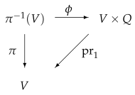
or, which is the same,

$$\pi ={\mathrm{pr}}_1\circ \varphi$$

on ${\pi }^{-1}\left(V\right)$. Sometimes, when a continuous mapping $\pi :Y\to X$ is given and no confusion may arise, $(V,\varphi )$, or just $\varphi$, is called a Q-trivialisation of Y over V. We also say that Y is Q-trivial over V.

Clearly, for any $x\in V$, the fibre ${\pi }^{-1}\left(x\right)$ is homeomorphic with Q.

A Q-trivialisation is said to be global if $V=X$. Existence of a global Q-trivialisation means that Y is homeomorphic with the Cartesian product $X\times Q$.

By a Q-fibration structure on a topological space Y, we mean a topological space X, a continuous surjective mapping $\pi :Y\to X$ and a family ${\left\{(V_{\iota },{\varphi }_{\iota })\right\}}_{\iota \in I}$ of Q-trivialisations of $\pi$ such that the family ${\left\{V_{\iota }\right\}}_{\iota \in I}$ covers X.

A topological space Y endowed with a Q-fibration structure $\pi :Y\to X$, ${\left\{(V_{\iota },{\varphi }_{\iota })\right\}}_{\iota \in I}$, is called a Q-fibration. Q is the type fibre, X is the base and $\pi$ is the projection of Y. The family ${\left\{(V_{\iota },{\varphi }_{\iota })\right\}}_{\iota \in I}$ is called the atlas of the Q-fibration Y.

The following is an immediate consequence of the definitions.

Lemma 1.

The projection π is an open mapping.

Proof. 

Standard. □

In the following lemma, we show that the topology of the base X of a Q-fibration Y is uniquely determined by the topology of Y.

The final topology associated with $\pi$ is a topology on X, formed by the sets $V\subset X$, such that ${\pi }^{-1}\left(V\right)$ is open in Y. Denote this topology by $\kappa$. Clearly, $\kappa$ is the strongest topology on X in which $\pi$ is continuous: if $\pi$ is continuous with respect to a different topology $\tau$ on X, then necessarily $\tau \subset \kappa$.

Lemma 2.

The topology of the base X of a Q-fibration Y coincides with the final topology associated with the Q-projection $\pi :Y\to X$.

Proof. 

Let $\tau$ be the topology of X, and let $\kappa$ be the final topology associated with $\pi$. Let $V\in \kappa$. Then, ${\pi }^{-1}\left(V\right)$ is open in Y. Since $\pi$ is open, the set $\pi \left({\pi }^{-1}\left(V\right)\right)$ is open in the topology $\tau$. But by surjectivity of $\pi$, $\pi \left({\pi }^{-1}\left(V\right)\right)=V$; thus, $\kappa \subset \tau$. On the other hand since $\tau \subset \kappa$, we have $\kappa =\tau$. □

Let ${\left\{(V_{\iota },{\varphi }_{\iota })\right\}}_{\iota \in I}$ be an atlas of a Q-fibration Y. Consider any two charts $(V_{\iota },{\varphi }_{\iota })$, ${\varphi }_{\iota }:{\pi }^{-1}\left(V_{\iota }\right)\to V_{\iota }\times Q$, and $(V_{\kappa },{\varphi }_{\kappa })$, ${\varphi }_{\kappa }:{\pi }^{-1}\left(V_{\kappa }\right)\to V_{\kappa }\times Q$, such that $V_{\iota }\cap V_{\kappa }\ne \varnothing$. Then, for every point $y\in {\pi }^{-1}\left(V_{\iota }\right)\cap {\pi }^{-1}\left(V_{\kappa }\right)$,

$${\varphi }_{\iota }\left(y\right)=(\pi \left(y\right),{\tilde{\varphi }}_{\iota }\left(y\right)),{\varphi }_{\kappa }\left(y\right)=(\pi \left(y\right),{\tilde{\varphi }}_{\kappa }\left(y\right))$$

hence $y\in {\varphi }_{\kappa }^{-1}(\pi \left(y\right),{\tilde{\varphi }}_{\kappa }\left(y\right))={\varphi }_{\iota }^{-1}(\pi \left(y\right),{\tilde{\varphi }}_{\iota }\left(y\right))$. Thus,

$$(\pi \left(y\right),{\tilde{\varphi }}_{\kappa }\left(y\right))={\varphi }_{\kappa }{\varphi }_{\iota }^{-1}(\pi \left(y\right),{\tilde{\varphi }}_{\iota }\left(y\right)),$$

and

$${\mathrm{pr}}_1(\pi \left(y\right),{\tilde{\varphi }}_{\kappa }\left(y\right))=\pi \left(y\right)={\mathrm{pr}}_1{\varphi }_{\kappa }{\varphi }_{\iota }^{-1}(\pi \left(y\right),{\tilde{\varphi }}_{\iota }\left(y\right)).$$

These formulas define a homeomorphism ${\varphi }_{\kappa }{\varphi }_{\iota }^{-1}:(V_{\iota }\cap V_{\kappa })\times Q\to (V_{\iota }\cap V_{\kappa })\times Q$, the transition homeomorphism between the Q-fibration charts $(V_{\iota },{\varphi }_{\iota })$, and $(V_{\kappa },{\varphi }_{\kappa })$. This homeomorphism is represented by a commutative diagram

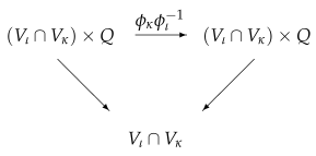
That is, in particular,

$${\varphi }_{\kappa }{\varphi }_{\iota }^{-1}(x,q)=(x,{\varphi }_{\kappa \iota }(x,q)),$$

(1)

on $(V_{\iota }\cap V_{\kappa })\times Q$, where for every $x\in V_{\iota }\cap V_{\kappa }$ the mapping ${\varphi }_{\kappa \iota }$ restricted to the fibre over x is a homeomorphism of Q. In other words, the family ${\varphi }_{\kappa \iota }(x,q)$ labelled by $x\in V_{\iota }\cap V_{\kappa }$ is a family of homeomorphisms of Q.

3. Actions of Topological Groups

3.1. Actions of Topological Groups on Topological Spaces

A group structure and a topological structure on a set G are said to be compatible if the group multiplication $G\times G\ni (g,h)\to g·h\in G$ and the inversion $G\ni g\to g^{-1}\in G$ are continuous. By a topological group we mean a set endowed with compatible group and topological structures.

Let G be a topological group and $e_G$ the identity element of G. By a right action of G on a topological space Y we mean a continuous mapping $Y\times G\ni (y,g)\to y·g\in Y$ such that $y·(g·h)=(y·g)·h$ and $y·e_G=y$ for all $y\in Y$ and all $g,h\in G$. The G-orbits of the points $y_0\in Y$, $y_0·G=\{y\in Y\mid y=y_0·g,g\in G\}$ are equivalence classes of equivalence relation “$y_1\sim y_2$ if there exists $g\in G$ such that $y_2=y_1·g$”; the corresponding quotient set is denoted by $Y/G$, and $\pi :Y\to Y/G$ is the corresponding quotient projection. The set $Y/G$, endowed with the quotient topology, the strongest topology in which $\pi$ is continuous, is called the orbit space.

$\pi$ is an open mapping. Indeed, for an open set $V\subset X$, its saturation

$${\pi }^{-1}\left(\pi \left(V\right)\right)=\bigcup _{g\in G}V·g$$

is a union of open sets $V·g$ and is therefore open; then, however, $\pi \left(V\right)$ is by definition open in the quotient topology.

Any point $y\in Y$ defines a surjective mapping $G\ni g\to {\mathsf{\Theta }}_y\left(g\right)=y·g\in Y$ called the G-orbit mapping passing through the point y. Clearly, ${\mathsf{\Theta }}_y$ is continuous and

$${\mathsf{\Theta }}_y\left(gh\right)=y·\left(gh\right)=(y·g)·h={\mathsf{\Theta }}_y\left(g\right)·h.$$

Analogously, by a left action of G on a topological space Y we mean a continuous mapping $G\times Y\ni (g,y)\to g·y\in Y$ such that $(g·h)·y=g·(h·y)$ and $e_G·y=y$ for all $y\in Y$ and all $g,h\in G$. The concepts of a G-orbit and the orbit space $Y/G$ of a left action are defined as in the case of a right action.

Given a left action $(g,y)\to g·y$, any point $y\in Y$ defines a surjective mapping $G\ni g\to {\mathsf{\Theta }}_y\left(g\right)=g·y\in Y$ called the G-orbit mapping passing through $y\in Y$. Clearly, ${\mathsf{\Theta }}_y$ is continuous and

$${\mathsf{\Theta }}_y\left(gh\right)=\left(gh\right)·y=g·(h·y)=g·{\mathsf{\Theta }}_y\left(h\right).$$

(2)

The right and left group actions may have additional properties. In the next two subsections, specific cases needed in this article are introduced.

3.2. Principal G-Bundles

A right action $Y\times G\ni (y,g)\to y·g\in Y$ is said to be free if for any $y\in Y$, the equation $y·g=y$ has a unique solution $g=e_G$; equivalently, we say that G acts on Y freely, or without fixed points.

A right action $Y\times G\ni (y,g)\to y·g\in Y$ is said to be principal if it is free and the following local triviality condition is satisfied: For every point $y_0\in Y$ there exist a G-invariant neighbourhood W of $y_0$ and a homeomorphism $\varphi :W\to \pi \left(W\right)\times G$ such that for all $y\in W$ and all $g\in G$

$$\pi \left(y\right)={\mathrm{pr}}_1\circ \varphi \left(y\right)$$

(3)

and

$$\varphi (y·g)=\varphi \left(y\right)·g.$$

A topological space Y endowed with a principal right action of a topological group G is called a principal G-bundle, or just a principal bundle if no misunderstanding may arise. G is called the structure group, the orbit space $Y/G$ the base and the quotient projection $\pi :Y\to Y/G$ the projection of the principal G-bundle Y.

Clearly, a principal G-bundle is a G-fibration. The $\pi$-saturated sets are exactly the G-invariant sets; the G-trivialisations are the homeomorphisms $\varphi :W\to \pi \left(W\right)\times G$.

Remark 1.

For any topological space X and any topological group G, the canonical right group action $(X\times G)\times G\ni \left(\right(x,h),g)\to (x,h·g)\in X\times G$ of G on the Cartesian product $X\times G$ is principal, and defines on $X\times G$ the canonical principal G-bundle structure.

By a principal G-bundle chart on a principal G-bundle Y we mean any pair $(W,\varphi )$, where W is a G-invariant open set in Y and $\varphi :V\to \pi \left(V\right)\times G$ is a G-equivariant G-trivialisation. An atlas for Y is a collection ${\left\{(W_{\iota },{\mathsf{\Phi }}_{\iota })\right\}}_{\iota \in I}$ of principal G-bundle charts such that ${\bigcup }_{\iota \in I}{W}_{\iota }=Y$.

We shall determine the transition homeomorphisms (1) for a principal G-bundle atlas ${\left\{(W_{\iota },{\varphi }_{\iota })\right\}}_{\iota \in I}$. Denote $V_{\iota }=\pi \left(W_{\iota }\right)$ for all $\iota \in I$ and express ${\varphi }_{\iota }$ as

$${\varphi }_{\iota }=(\pi ,{\tilde{\varphi }}_{\iota }),$$

(4)

where ${\tilde{\varphi }}_{\iota }$ is the principal part of the G-trivialisation ${\varphi }_{\iota }$. Conditions (2) and (3) imply

$${\tilde{\varphi }}_{\iota }(y·g)={\tilde{\varphi }}_{\iota }\left(y\right)·g$$

for all $y\in W_{\iota }$ and all $g\in G$.

Lemma 3.

For any two principal G-bundle charts $(W_{\iota },{\varphi }_{\iota })$ and $(W_{\kappa },{\varphi }_{\kappa })$ such that $W_{\iota }\cap W_{\kappa }\ne \varnothing$, the mapping $W_{\iota }\cap W_{\kappa }\ni y={\tilde{\varphi }}_{\kappa }\left(y\right)·{\tilde{\varphi }}_{\iota }^{-1}\left(y\right)\in G$ is constant along the fibres ${\pi }^{-1}\left(x\right)$ over $x\in V_{\iota }\cap V_{\kappa }$.

Proof. 

Let $x\in V_{\iota }\cap V_{\kappa }$ and let $y,y^{\prime }\in {\pi }^{-1}\left(x\right)$. Then, $y^{\prime }=y·g$ for some $g\in G$; hence, by (4),

$$\begin{array}{c}{\tilde{\varphi }}_{\kappa }\left(y^{\prime }\right)·{\tilde{\varphi }}_{\iota }^{-1}\left(y^{\prime }\right)={\tilde{\varphi }}_{\kappa }(y·g)·{\tilde{\varphi }}_{\iota }^{-1}(y·g)={\tilde{\varphi }}_{\kappa }·g·g^{-1}·{\tilde{\varphi }}_{\iota }^{-1}\left(y\right)\\ ={\tilde{\varphi }}_{\kappa }\left(y\right)·{\tilde{\varphi }}_{\iota }^{-1}\left(y\right).\end{array}$$

(5)

□

Set for any $x\in V_{\iota }\cap V_{\kappa }$ and any $y\in {\pi }^{-1}\left(x\right)$

$${\varphi }_{\kappa \iota }\left(x\right)={\tilde{\varphi }}_{\kappa }\left(y\right)·{\tilde{\varphi }}_{\iota }^{-1}\left(y\right).$$

(6)

By Lemma 3, Formula (5) defines a continuous mapping $V_{\iota }\cap V_{\kappa }\ni x\to {\varphi }_{\kappa \iota }\left(x\right)\in G$.

Lemma 4.

The transition homeomorphism ${\varphi }_{\kappa }{\varphi }_{\iota }^{-1}:(V_{\iota }\cap V_{\kappa })\times G\to (V_{\iota }\cap V_{\kappa })\times G$ is of the form

$${\varphi }_{\kappa }{\varphi }_{\iota }^{-1}(x,h)=(x,{\varphi }_{\kappa \iota }\left(x\right)·h).$$

Proof. 

By definition ${\varphi }_{\iota }\left(y\right)=(\pi \left(y\right),{\tilde{\varphi }}_{\iota }\left(y\right))$, ${\varphi }_{\kappa }\left(y\right)=(\pi \left(y\right),{\tilde{\varphi }}_{\kappa }\left(y\right))$, and using (5)

$$\begin{array}{c}{\varphi }_{\kappa }\left(y\right)=(\pi \left(y\right),{\tilde{\varphi }}_{\kappa }\left(y\right)·{\tilde{\varphi }}_{\iota }^{-1}\left(y\right)·{\tilde{\varphi }}_{\iota }\left(y\right))\hfill \\ =(\pi \left(y\right),{\varphi }_{\kappa \iota }\left(x\right)·{\tilde{\varphi }}_{\iota }\left(y\right)).\hfill \end{array}$$

But also ${\varphi }_{\kappa }\left(y\right)={\varphi }_{\kappa }{\varphi }_{\iota }^{-1}{\varphi }_{\iota }\left(y\right)={\varphi }_{\kappa }{\varphi }_{\iota }^{-1}(\pi \left(y\right),{\tilde{\varphi }}_{\iota }\left(y\right))$; hence, ${\varphi }_{\kappa }{\varphi }_{\iota }^{-1}(x,h)=(x,{\varphi }_{\kappa \iota }\left(x\right)·h)$ as required. □

Remark 2.

For $h=e_G$ transition G-homeomorphisms (6), determine sections $x\to (x,{\varphi }_{\kappa \iota }\left(x\right))$ of the trivial principal G-bundles $(V_{\iota }\cap V_{\kappa })\times G$. Thus, a necessary and sufficient condition for the principal G-bundle Y to be trivial is the existence of a global continuous section of Y.

3.3. Left Actions: Subgroup Orbit Structure

The orbit stabilizer theorem as formulated in Krupka and Brajerčík [1], Section 2.3, can be easily extended to topological groups. Recall basic concepts within the category of topological spaces. Let Y be a topological space endowed with a continuous left action of a topological group G. Choose $y_0\in Y$ and set, for every $g\in G$,

$${\mathsf{\Theta }}_{y_0}\left(g\right)=g·y_0.$$

${\mathsf{\Theta }}_{y_0}:G\to G{y}_0$ is the G-orbit mapping passing through the point $y_0$. Clearly, ${\mathsf{\Theta }}_{y_0}\left(g_1{g}_2\right)=g_1·{\mathsf{\Theta }}_{y_0}\left(g_2\right)$ for all $g_1,g_2\in G$; in particular, ${\mathsf{\Theta }}_{y_0}$ is G-equivariant.

As before, let $G_{y_0}$ be the orbit stabilizer of the point $y_0$. If $h\in G_{y_0}$, then ${\mathsf{\Theta }}_{y_0}\left(h\right)=y_0$.

Lemma 5.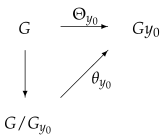

For any point $y_0\in Y$, there exists a unique G-equivariant homeomorphism ${\theta }_{y_0}:G/G_{y_0}\to G{y}_0$ such that the diagram

commutes.

4. Principal Bundle Structure of SO(3)

4.1. The SO(2)-Fibration Structure on SO(3)

Recall the definition of the cross-product mapping $\chi :\mathsf{S}\mathsf{O}\left(3\right)\to S^2$ (Krupka, Brajerčík [1], Section 3.3). For any special orthogonal matrix $\tau \in \mathsf{S}\mathsf{O}\left(3\right)$ expressed by

$$\tau =\left(\begin{array}{ccc}{x}_1& x_2& x_3\\ y_1& y_2& y_3\\ z_1& z_2& z_3\end{array}\right)$$

(7)

$\chi \left(\tau \right)$ is defined to be the first column vector in $\tau$; for convenience, we also write $\chi \left(\tau \right)$ as a raw vector,

$$\chi \left(\tau \right)=\left(x_1,y_1,z_1\right).$$

(8)

By special orthogonality of $\tau$,

$$x_1=\left|\begin{array}{cc}{y}_2& y_3\\ z_2& z_3\end{array}\right|,y_1=-\left|\begin{array}{cc}{x}_2& x_3\\ z_2& z_3\end{array}\right|,z_1=\left|\begin{array}{cc}{x}_2& x_3\\ y_2& y_3\end{array}\right|.$$

$\chi$ can also be viewed as the restriction to SO(3) of the Cartesian projection of a $(3\times 3)$-matrix onto its first column followed by the restriction of its range ${\mathbf{R}}^3$ to its image $S^2$. $\chi$ is obviously surjective and continuous.

Our objective in this subsection is to demonstrate that the cross-product mapping $\chi$ defines on SO(3) the structure of an SO(2)-fibration.

We consider ${\mathbf{R}}^3$ with its canonical coordinates x, y and z; then, the unit sphere $S^2\subset {\mathbf{R}}^3$ is the set $S^2=\{(x,y,z)\in {\mathbf{R}}^3\mid x^2+y^2+z^2=1\}$. Our constructions are based on an observation that any vector $(x,y,z)\in {\mathbf{R}}^3$, such that $x^2+y^2+z^2=1$ and $-1<x<1$, satisfies

$${\left({\displaystyle \frac{y}{\sqrt{1-x^2}}}\right)}^2+{\left({\displaystyle \frac{z}{\sqrt{1-x^2}}}\right)}^2={\displaystyle \frac{y^2+z^2}{\sqrt{1-x^2}}}=1.$$

In particular, we have a mapping

$$\{(x,y,z)\in S^2\mid -1<x<1\}\ni (x,y,z)\to \left(\begin{array}{cc}{\displaystyle \frac{y}{\sqrt{1-x^2}}}& -{\displaystyle \frac{z}{\sqrt{1-x^2}}}\\ {\displaystyle \frac{z}{\sqrt{1-x^2}}}& {\displaystyle \frac{y}{\sqrt{1-x^2}}}\end{array}\right)\in \mathsf{S}\mathsf{O}\left(2\right)$$

or, in an obvious sense, a section of the cross-product $\chi :\mathsf{S}\mathsf{O}\left(3\right)\to S^2$ over the set where $-1<x<1$. Analogous sections arise on the subsets of the sphere $S^2$ where $-1<y<1$ or $-1<z<1$.

Recall that the cyclic permutation matrices ${\nu }_1,{\nu }_2,{\nu }_3$ are defined by

$${\nu }_1=\left(\begin{array}{ccc}1& 0& 0\\ 0& 1& 0\\ 0& 0& 1\end{array}\right),{\nu }_2=\left(\begin{array}{ccc}0& 0& 1\\ 1& 0& 0\\ 0& 1& 0\end{array}\right),{\nu }_3=\left(\begin{array}{ccc}0& 1& 0\\ 0& 0& 1\\ 1& 0& 0\end{array}\right).$$

These matrices constitute a subgroup of SO(3). The group multiplication yields ${\nu }_2{\nu }_3={\nu }_1$. For any $\tau \in \mathsf{S}\mathsf{O}\left(3\right)$ written as (7), we have

$${\nu }_1\tau =\left(\begin{array}{ccc}{x}_1& x_2& x_3\\ y_1& y_2& y_3\\ z_1& z_2& z_3\end{array}\right),{\nu }_2\tau =\left(\begin{array}{ccc}{z}_1& z_2& z_3\\ x_1& x_2& x_3\\ y_1& y_2& y_3\end{array}\right),{\nu }_3\tau =\left(\begin{array}{ccc}{y}_1& y_2& y_3\\ z_1& z_2& z_3\\ x_1& x_2& x_3\end{array}\right).$$

In particular, if

$$\tau =\left(\begin{array}{ccc}1& 0& 0\\ 0& y_2& y_3\\ 0& z_2& z_3\end{array}\right),$$

then

$${\nu }_1\tau =\left(\begin{array}{ccc}1& 0& 0\\ 0& y_2& y_3\\ 0& z_2& z_3\end{array}\right),{\nu }_2\tau =\left(\begin{array}{ccc}0& z_2& z_3\\ 1& 0& 0\\ 0& y_2& y_3\end{array}\right),{\nu }_3\tau =\left(\begin{array}{ccc}0& y_2& y_3\\ 0& z_2& z_3\\ 1& 0& 0\end{array}\right).$$

Lemma 6.

Any matrix $\tau \in \mathsf{SO}\left(3\right)$ admits the following decompositions in the group SO(3):

(a) If $-1<z_1<1$, then

$$\left(\begin{array}{ccc}{x}_1& x_2& x_3\\ y_1& y_2& y_3\\ z_1& z_2& z_3\end{array}\right)=\left(\begin{array}{ccc}{x}_1& -{\displaystyle \frac{y_1}{\sqrt{1-z_1^2}}}& -{\displaystyle \frac{x_1{z}_1}{\sqrt{1-z_1^2}}}\\ y_1& {\displaystyle \frac{x_1}{\sqrt{1-z_1^2}}}& -{\displaystyle \frac{y_1{z}_1}{\sqrt{1-z_1^2}}}\\ z_1& 0& \sqrt{1-z_1^2}\end{array}\right)\left(\begin{array}{ccc}1& 0& 0\\ 0& {\displaystyle \frac{z_3}{\sqrt{1-z_1^2}}}& -{\displaystyle \frac{z_2}{\sqrt{1-z_1^2}}}\\ 0& {\displaystyle \frac{z_2}{\sqrt{1-z_1^2}}}& {\displaystyle \frac{z_3}{\sqrt{1-z_1^2}}}\end{array}\right).$$

(9)

(b) If $-1<y_1<1$, then

$$\left(\begin{array}{ccc}{x}_1& x_2& x_3\\ y_1& y_2& y_3\\ z_1& z_2& z_3\end{array}\right)=\left(\begin{array}{ccc}{x}_1& {\displaystyle \frac{z_1}{\sqrt{1-y_1^2}}}& -{\displaystyle \frac{x_1{y}_1}{\sqrt{1-y_1^2}}}\\ y_1& 0& \sqrt{1-y_1^2}\\ z_1& -{\displaystyle \frac{x_1}{\sqrt{1-y_1^2}}}& -{\displaystyle \frac{y_1{z}_1}{\sqrt{1-y_1^2}}}\end{array}\right)\left(\begin{array}{ccc}1& 0& 0\\ 0& {\displaystyle \frac{y_3}{\sqrt{1-y_1^2}}}& -{\displaystyle \frac{y_2}{\sqrt{1-y_1^2}}}\\ 0& {\displaystyle \frac{y_2}{\sqrt{1-y_1^2}}}& {\displaystyle \frac{y_3}{\sqrt{1-y_1^2}}}\end{array}\right).$$

(10)

(c) If $-1<x_1<1$, then

$$\left(\begin{array}{ccc}{x}_1& x_2& x_3\\ y_1& y_2& y_3\\ z_1& z_2& z_3\end{array}\right)=\left(\begin{array}{ccc}{x}_1& 0& \sqrt{1-x_1^2}\\ y_1& -{\displaystyle \frac{z_1}{\sqrt{1-x_1^2}}}& -{\displaystyle \frac{x_1{y}_1}{\sqrt{1-x_1^2}}}\\ z_1& {\displaystyle \frac{y_1}{\sqrt{1-x_1^2}}}& -{\displaystyle \frac{x_1{z}_1}{\sqrt{1-x_1^2}}}\end{array}\right)\left(\begin{array}{ccc}1& 0& 0\\ 0& {\displaystyle \frac{x_3}{\sqrt{1-x_1^2}}}& -{\displaystyle \frac{x_2}{\sqrt{1-x_1^2}}}\\ 0& {\displaystyle \frac{x_2}{\sqrt{1-x_1^2}}}& {\displaystyle \frac{x_3}{\sqrt{1-x_1^2}}}\end{array}\right).$$

(11)

Proof. 

(a) Clearly, under assumption $-1<z_1<1$, the matrix

$$\left(\begin{array}{ccc}1& 0& 0\\ 0& {\displaystyle \frac{z_3}{\sqrt{1-z_1^2}}}& -{\displaystyle \frac{z_2}{\sqrt{1-z_1^2}}}\\ 0& {\displaystyle \frac{z_2}{\sqrt{1-z_1^2}}}& {\displaystyle \frac{z_3}{\sqrt{1-z_1^2}}}\end{array}\right).$$

satisfies $z_2^2+z_3^2=1-z_1^2$ and $z_3{z}_2-z_2{z}_3=0$, so it is special orthogonal. Since the inverse of a special orthogonal matrix coincides with its transpose, we have the identity

$$\begin{array}{c}\left(\begin{array}{ccc}{x}_1& x_2& x_3\\ y_1& y_2& y_3\\ z_1& z_2& z_3\end{array}\right)\\ =\left(\begin{array}{ccc}{x}_1& x_2& x_3\\ y_1& y_2& y_3\\ z_1& z_2& z_3\end{array}\right)\left(\begin{array}{ccc}1& 0& 0\\ 0& {\displaystyle \frac{z_3}{\sqrt{1-z_1^2}}}& {\displaystyle \frac{z_2}{\sqrt{1-z_1^2}}}\\ 0& -{\displaystyle \frac{z_2}{\sqrt{1-z_1^2}}}& {\displaystyle \frac{z_3}{\sqrt{1-z_1^2}}}\end{array}\right)\left(\begin{array}{ccc}1& 0& 0\\ 0& {\displaystyle \frac{z_3}{\sqrt{1-z_1^2}}}& -{\displaystyle \frac{z_2}{\sqrt{1-z_1^2}}}\\ 0& {\displaystyle \frac{z_2}{\sqrt{1-z_1^2}}}& {\displaystyle \frac{z_3}{\sqrt{1-z_1^2}}}\end{array}\right).\end{array}$$

(12)

Calculating the product of the first two matrices,

$$\left(\begin{array}{ccc}{x}_1& x_2& x_3\\ y_1& y_2& y_3\\ z_1& z_2& z_3\end{array}\right)\left(\begin{array}{ccc}1& 0& 0\\ 0& {\displaystyle \frac{z_3}{\sqrt{1-z_1^2}}}& {\displaystyle \frac{z_2}{\sqrt{1-z_1^2}}}\\ 0& -{\displaystyle \frac{z_2}{\sqrt{1-z_1^2}}}& {\displaystyle \frac{z_3}{\sqrt{1-z_1^2}}}\end{array}\right)=\left(\begin{array}{ccc}{x}_1& {\displaystyle \frac{x_2{z}_3-x_3{z}_2}{\sqrt{1-z_1^2}}}& {\displaystyle \frac{x_2{z}_2+x_3{z}_3}{\sqrt{1-z_1^2}}}\\ y_1& {\displaystyle \frac{y_2{z}_3-y_3{z}_2}{\sqrt{1-z_1^2}}}& {\displaystyle \frac{y_2{z}_2+y_3{z}_3}{\sqrt{1-z_1^2}}}\\ z_1& {\displaystyle \frac{z_2{z}_3-z_3{z}_2}{\sqrt{1-z_1^2}}}& {\displaystyle \frac{z_2^2+z_3^2}{\sqrt{1-z_1^2}}}\end{array}\right).$$

(13)

But from

$$\begin{array}{c}{x}_2{z}_3-x_3{z}_2=\left|\begin{array}{cc}{x}_2& x_3\\ z_2& z_3\end{array}\right|=-y_1,y_2{z}_3-y_3{z}_2=\left|\begin{array}{cc}{y}_2& y_3\\ z_2& z_3\end{array}\right|=x_1,\\ z_2{z}_3-z_3{z}_2=0\end{array}$$

and from the orthogonality conditions

$$x_2{z}_2+x_3{z}_3=-x_1{z}_1,y_2{z}_2+y_3{z}_3=-y_1{z}_1,z_2^2+z_3^2=1-z_1^2$$

hence

$$\left(\begin{array}{ccc}{x}_1& {\displaystyle \frac{x_2{z}_3-x_3{z}_2}{\sqrt{1-z_1^2}}}& {\displaystyle \frac{x_2{z}_2+x_3{z}_3}{\sqrt{1-z_1^2}}}\\ y_1& {\displaystyle \frac{y_2{z}_3-y_3{z}_2}{\sqrt{1-z_1^2}}}& {\displaystyle \frac{y_2{z}_2+y_3{z}_3}{\sqrt{1-z_1^2}}}\\ z_1& {\displaystyle \frac{z_2{z}_3-z_3{z}_2}{\sqrt{1-z_1^2}}}& {\displaystyle \frac{z_2^2+z_3^2}{\sqrt{1-z_1^2}}}\end{array}\right)=\left(\begin{array}{ccc}{x}_1& -{\displaystyle \frac{y_1}{\sqrt{1-z_1^2}}}& -{\displaystyle \frac{x_1{z}_1}{\sqrt{1-z_1^2}}}\\ y_1& {\displaystyle \frac{x_1}{\sqrt{1-z_1^2}}}& -{\displaystyle \frac{y_1{z}_1}{\sqrt{1-z_1^2}}}\\ z_1& 0& \sqrt{1-z_1^2}\end{array}\right).$$

This formula already proves (9).

(b) If $-1<y_1<1$, we repeat the calculation in part (a) of this proof for the matrix

$${\nu }_2\tau =\left(\begin{array}{ccc}{z}_1& z_2& z_3\\ x_1& x_2& x_3\\ y_1& y_2& y_3\end{array}\right).$$

Performing the corresponding replacements in (9),

$$\left(\begin{array}{ccc}{z}_1& z_2& z_3\\ x_1& x_2& x_3\\ y_1& y_2& y_3\end{array}\right)=\left(\begin{array}{ccc}{z}_1& -{\displaystyle \frac{x_1}{\sqrt{1-y_1^2}}}& -{\displaystyle \frac{z_1{y}_1}{\sqrt{1-y_1^2}}}\\ x_1& {\displaystyle \frac{z_1}{\sqrt{1-y_1^2}}}& -{\displaystyle \frac{x_1{y}_1}{\sqrt{1-y_1^2}}}\\ y_1& 0& \sqrt{1-y_1^2}\end{array}\right)\left(\begin{array}{ccc}1& 0& 0\\ 0& {\displaystyle \frac{y_3}{\sqrt{1-y_1^2}}}& -{\displaystyle \frac{y_2}{\sqrt{1-y_1^2}}}\\ 0& {\displaystyle \frac{y_2}{\sqrt{1-y_1^2}}}& {\displaystyle \frac{y_3}{\sqrt{1-y_1^2}}}\end{array}\right).$$

To return to $\tau$, we multiply ${\nu }_2\tau$ by ${\nu }_3={\nu }_2^{-1}$. Since

$${\nu }_3=\left(\begin{array}{ccc}0& 1& 0\\ 0& 0& 1\\ 1& 0& 0\end{array}\right),$$

then

$$\begin{array}{c}\tau ={\nu }_3{\nu }_2\tau \\ =\left(\begin{array}{ccc}0& 1& 0\\ 0& 0& 1\\ 1& 0& 0\end{array}\right)\left(\begin{array}{ccc}{z}_1& -{\displaystyle \frac{x_1}{\sqrt{1-y_1^2}}}& -{\displaystyle \frac{z_1{y}_1}{\sqrt{1-y_1^2}}}\\ x_1& {\displaystyle \frac{z_1}{\sqrt{1-y_1^2}}}& -{\displaystyle \frac{x_1{y}_1}{\sqrt{1-y_1^2}}}\\ y_1& 0& \sqrt{1-y_1^2}\end{array}\right)\left(\begin{array}{ccc}1& 0& 0\\ 0& {\displaystyle \frac{y_3}{\sqrt{1-y_1^2}}}& -{\displaystyle \frac{y_2}{\sqrt{1-y_1^2}}}\\ 0& {\displaystyle \frac{y_2}{\sqrt{1-y_1^2}}}& {\displaystyle \frac{y_3}{\sqrt{1-y_1^2}}}\end{array}\right)\\ =\left(\begin{array}{ccc}{x}_1& {\displaystyle \frac{z_1}{\sqrt{1-y_1^2}}}& -{\displaystyle \frac{x_1{y}_1}{\sqrt{1-y_1^2}}}\\ y_1& 0& \sqrt{1-y_1^2}\\ z_1& -{\displaystyle \frac{x_1}{\sqrt{1-y_1^2}}}& -{\displaystyle \frac{z_1{y}_1}{\sqrt{1-y_1^2}}}\end{array}\right)\left(\begin{array}{ccc}1& 0& 0\\ 0& {\displaystyle \frac{y_3}{\sqrt{1-y_1^2}}}& -{\displaystyle \frac{y_2}{\sqrt{1-y_1^2}}}\\ 0& {\displaystyle \frac{y_2}{\sqrt{1-y_1^2}}}& {\displaystyle \frac{y_3}{\sqrt{1-y_1^2}}}\end{array}\right)\end{array}$$

proving (10).

(c) Replace ${\nu }_2$ in part (b) of the proof by the permutation matrix ${\nu }_3$. □

Denote

$$\begin{array}{c}{W}_3=\{\tau \in \mathsf{S}\mathsf{O}\left(3\right)\mid -1<z_1<1\},\\ W_2=\{\tau \in \mathsf{S}\mathsf{O}\left(3\right)\mid -1<y_1<1\},\\ W_1=\{\tau \in \mathsf{S}\mathsf{O}\left(3\right)\mid -1<x_1<1\},\end{array}$$

and

$$\begin{array}{c}{V}_3=\{(x_1,y_1,z_1)\in S^2\mid -1<z_1<1\},\\ V_2=\{(x_1,y_1,z_1)\in S^2\mid -1<y_1<1\},\\ V_1=\{(x_1,y_1,z_1)\in S^2\mid -1<x_1<1\}.\end{array}$$

$W_3,W_2,W_1$ are open sets in SO(3), $V_3,V_2,V_1$ are open sets in $S^2$, and

$$\begin{array}{c}\chi \left(W_3\right)=V_3,\chi \left(W_2\right)=V_2,\chi \left(W_1\right)=V_1,\\ W_3={\chi }^{-1}\left(V_3\right),W_2={\chi }^{-1}\left(V_2\right),W_1={\chi }^{-1}\left(V_1\right).\end{array}$$

Consider the mappings

$$W_3\ni \tau \to {\varphi }_3\left(\tau \right)=\left((x_1,y_1,z_1),\left(\begin{array}{ccc}1& 0& 0\\ 0& {\displaystyle \frac{z_3}{\sqrt{1-z_1^2}}}& -{\displaystyle \frac{z_2}{\sqrt{1-z_1^2}}}\\ 0& {\displaystyle \frac{z_2}{\sqrt{1-z_1^2}}}& {\displaystyle \frac{z_3}{\sqrt{1-z_1^2}}}\end{array}\right)\right)\in V_3\times \mathsf{S}\mathsf{O}\left(2\right),$$

(14)

$$W_2\ni \tau \to {\varphi }_2\left(\tau \right)=\left((x_1,y_1,z_1),\left(\begin{array}{ccc}1& 0& 0\\ 0& {\displaystyle \frac{y_3}{\sqrt{1-y_1^2}}}& -{\displaystyle \frac{y_2}{\sqrt{1-y_1^2}}}\\ 0& {\displaystyle \frac{y_2}{\sqrt{1-y_1^2}}}& {\displaystyle \frac{y_3}{\sqrt{1-y_1^2}}}\end{array}\right)\right)\in V_2\times \mathsf{S}\mathsf{O}\left(2\right),$$

(15)

$$W_1\ni \tau \to {\varphi }_1\left(\tau \right)=\left((x_1,y_1,z_1),\left(\begin{array}{ccc}1& 0& 0\\ 0& {\displaystyle \frac{x_3}{\sqrt{1-x_1^2}}}& -{\displaystyle \frac{x_2}{\sqrt{1-x_1^2}}}\\ 0& {\displaystyle \frac{x_2}{\sqrt{1-x_1^2}}}& {\displaystyle \frac{x_3}{\sqrt{1-x_1^2}}}\end{array}\right)\right)\in V_1\times \mathsf{S}\mathsf{O}\left(2\right),$$

(16)

and the pairs $(V_1,{\varphi }_1)$, $(V_2,{\varphi }_2)$, $(V_3,{\varphi }_3)$.

Lemma 7.

The mappings ${\varphi }_3,{\varphi }_2,{\varphi }_1$ are homeomorphisms. The inverse mappings ${\psi }_3:V_3\times \mathsf{SO}\left(2\right)\to W_3$, ${\psi }_2:V_2\times \mathsf{SO}\left(2\right)\to W_2$, ${\psi }_1:V_1\times \mathsf{SO}\left(2\right)\to W_1$ are given by

$${\psi }_3\left((x_1,y_1,z_1),\left(\begin{array}{cc}a& -b\\ b& a\end{array}\right)\right)=\left(\begin{array}{ccc}{x}_1& -{\displaystyle \frac{y_1}{\sqrt{1-z_1^2}}}& -{\displaystyle \frac{x_1{z}_1}{\sqrt{1-z_1^2}}}\\ y_1& {\displaystyle \frac{x_1}{\sqrt{1-z_1^2}}}& -{\displaystyle \frac{y_1{z}_1}{\sqrt{1-z_1^2}}}\\ z_1& 0& \sqrt{1-z_1^2}\end{array}\right)\left(\begin{array}{ccc}1& 0& 0\\ 0& a& -b\\ 0& b& a\end{array}\right),$$

(17)

$${\psi }_2\left((x_1,y_1,z_1),\left(\begin{array}{cc}a& -b\\ b& a\end{array}\right)\right)=\left(\begin{array}{ccc}{x}_1& {\displaystyle \frac{z_1}{\sqrt{1-y_1^2}}}& -{\displaystyle \frac{x_1{y}_1}{\sqrt{1-y_1^2}}}\\ y_1& 0& \sqrt{1-y_1^2}\\ z_1& -{\displaystyle \frac{x_1}{\sqrt{1-y_1^2}}}& -{\displaystyle \frac{y_1{z}_1}{\sqrt{1-y_1^2}}}\end{array}\right)\left(\begin{array}{ccc}1& 0& 0\\ 0& a& -b\\ 0& b& a\end{array}\right),$$

(18)

$${\psi }_1\left((x_1,y_1,z_1),\left(\begin{array}{cc}a& -b\\ b& a\end{array}\right)\right)=\left(\begin{array}{ccc}{x}_1& 0& \sqrt{1-x_1^2}\\ y_1& -{\displaystyle \frac{z_1}{\sqrt{1-x_1^2}}}& -{\displaystyle \frac{x_1{y}_1}{\sqrt{1-y_1^2}}}\\ z_1& {\displaystyle \frac{y_1}{\sqrt{1-x_1^2}}}& -{\displaystyle \frac{x_1{z}_1}{\sqrt{1-y_1^2}}}\end{array}\right)\left(\begin{array}{ccc}1& 0& 0\\ 0& a& -b\\ 0& b& a\end{array}\right).$$

(19)

Proof. 

We show that ${\varphi }_1$, ${\varphi }_2$ and ${\varphi }_3$ are bijective. It is sufficient to verify that ${\varphi }_1$, ${\varphi }_2$ and ${\varphi }_3$ are surjective and ${\psi }_3={\varphi }_3^{-1}$, ${\psi }_2={\varphi }_2^{-1}$ and ${\psi }_1={\varphi }_1^{-1}$.

We prove the surjectivity of ${\varphi }_3$. Choose a point

$$\left((x_0,y_0,z_0),\left(\begin{array}{cc}a& -b\\ b& a\end{array}\right)\right)\in \chi \left(W_3\right)\times \mathsf{S}\mathsf{O}\left(2\right)$$

such that $-1<z_0<1$. Then, equation

$$\left((x_1,y_1,z_1),\left(\begin{array}{cc}{\displaystyle \frac{z_3}{\sqrt{1-z_1^2}}}& -{\displaystyle \frac{z_2}{\sqrt{1-z_1^2}}}\\ {\displaystyle \frac{z_2}{\sqrt{1-z_1^2}}}& {\displaystyle \frac{z_3}{\sqrt{1-z_1^2}}}\end{array}\right)\right)=\left((x_0,y_0,z_0),\left(\begin{array}{cc}a& -b\\ b& a\end{array}\right)\right)$$

has a unique solution

$$\begin{array}{c}{x}_1=x_0,y_1=y_0,z_1=z_0,\\ z_3=a\sqrt{1-z_0^2},z_2=b\sqrt{1-z_0^2}\end{array}$$

proving the surjectivity of ${\varphi }_3$. The same is obviously true for and ${\varphi }_1$ and ${\varphi }_2$.

Now, immediate verification shows that ${\psi }_3={\varphi }_3^{-1}$. Indeed, by (17)

$$\begin{array}{c}{\psi }_3{\varphi }_3\left(\tau \right)={\psi }_3\left((x_1,y_1,z_1),\left(\begin{array}{cc}{\displaystyle \frac{z_3}{\sqrt{1-z_1^2}}}& -{\displaystyle \frac{z_2}{\sqrt{1-z_1^2}}}\\ {\displaystyle \frac{z_2}{\sqrt{1-z_1^2}}}& {\displaystyle \frac{z_3}{\sqrt{1-z_1^2}}}\end{array}\right)\right)\\ =\left(\begin{array}{ccc}{x}_1& -{\displaystyle \frac{y_1}{\sqrt{1-z_1^2}}}& -{\displaystyle \frac{x_1{z}_1}{\sqrt{1-z_1^2}}}\\ y_1& {\displaystyle \frac{x_1}{\sqrt{1-z_1^2}}}& -{\displaystyle \frac{y_1{z}_1}{\sqrt{1-z_1^2}}}\\ z_1& 0& \sqrt{1-z_1^2}\end{array}\right)·\left(\begin{array}{ccc}1& 0& 0\\ 0& {\displaystyle \frac{z_3}{\sqrt{1-z_1^2}}}& -{\displaystyle \frac{z_2}{\sqrt{1-z_1^2}}}\\ 0& {\displaystyle \frac{z_2}{\sqrt{1-z_1^2}}}& {\displaystyle \frac{z_3}{\sqrt{1-z_1^2}}}\end{array}\right)=\left(\begin{array}{ccc}{x}_1& x_2& x_3\\ y_1& y_2& y_3\\ z_1& z_2& z_3\end{array}\right)\end{array}$$

proving that ${\psi }_3={\varphi }_3^{-1}$. Similarly, by (18) and (19), we get ${\psi }_2={\varphi }_2^{-1}$ and ${\psi }_1={\varphi }_1^{-1}$, respectively.

Finally, Formulas (14)–(16) and (17)–(19) show that ${\varphi }_3$, ${\varphi }_2$, ${\varphi }_1$ and ${\psi }_3$, ${\psi }_2$, ${\psi }_1$ are continuous, and hence homeomorphisms. □

We can now conclude this subsection by the following theorem.

Theorem 1.

The cross-product $\chi :\mathsf{SO}\left(3\right)\to S^2$ defines on $\mathsf{SO}\left(3\right)$ the structure of an $\mathsf{SO}\left(2\right)$-fibration.

Proof. 

It is immediately verified that the topological space SO(3), the mapping $\chi :\mathsf{SO}\left(3\right)\to S^2$ and the family of trivialisations $\{(V_1,{\varphi }_1),(V_2,{\varphi }_2),(V_3,{\varphi }_3)\}$ satisfy the axioms of an SO(2)-fibration. □

4.2. The Principal SO(2)-Bundle Structure on SO(3)

In this subsection, we consider a continuous right action of SO(2) on SO(3) given by

$$\begin{array}{c}\mathsf{S}\mathsf{O}\left(3\right)\times \mathsf{S}\mathsf{O}\left(2\right)\ni \left(\left(\begin{array}{ccc}{\tau }_{11}& {\tau }_{12}& {\tau }_{13}\\ {\tau }_{21}& {\tau }_{22}& {\tau }_{23}\\ {\tau }_{31}& {\tau }_{32}& {\tau }_{33}\end{array}\right),\left(\begin{array}{cc}{\nu }_{11}& {\nu }_{12}\\ {\nu }_{21}& {\nu }_{22}\end{array}\right)\right)\\ \to \left(\begin{array}{ccc}{\tau }_{11}& {\tau }_{12}& {\tau }_{13}\\ {\tau }_{21}& {\tau }_{22}& {\tau }_{23}\\ {\tau }_{31}& {\tau }_{32}& {\tau }_{33}\end{array}\right)·\left(\begin{array}{cc}{\nu }_{11}& {\nu }_{12}\\ {\nu }_{21}& {\nu }_{22}\end{array}\right)=\left(\begin{array}{ccc}{\tau }_{11}& {\tau }_{12}& {\tau }_{13}\\ {\tau }_{21}& {\tau }_{22}& {\tau }_{23}\\ {\tau }_{31}& {\tau }_{32}& {\tau }_{33}\end{array}\right)·\left(\begin{array}{ccc}1& 0& 0\\ 0& {\nu }_{11}& {\nu }_{12}\\ 0& {\nu }_{21}& {\nu }_{22}\end{array}\right)\in \mathsf{S}\mathsf{O}\left(3\right)\end{array}$$

(20)

We show that this right group action is principal and find an explicit formula for the corresponding quotient projection.

First, let us examine the equivalence relation on SO(3) “$\kappa \sim \tau$ if there exists a matrix $\nu \in \mathsf{S}\mathsf{O}\left(2\right)$ such that $\kappa =\tau ·\nu$”.

Lemma 8.

Let $\tau ,\kappa \in \mathsf{SO}\left(3\right)$ be any matrices,

$$\tau =\left(\begin{array}{ccc}{\tau }_{11}& {\tau }_{12}& {\tau }_{13}\\ {\tau }_{21}& {\tau }_{22}& {\tau }_{23}\\ {\tau }_{31}& {\tau }_{32}& {\tau }_{33}\end{array}\right),\kappa =\left(\begin{array}{ccc}{\kappa }_{11}& {\kappa }_{12}& {\kappa }_{13}\\ {\kappa }_{21}& {\kappa }_{22}& {\kappa }_{23}\\ {\kappa }_{31}& {\kappa }_{32}& {\kappa }_{33}\end{array}\right).$$

(21)

The following conditions are equivalent:

(a)$\kappa =\tau ·\nu$ for some $\nu \in \mathsf{SO}\left(2\right)$.

(b)The entries of τ and κ satisfy

$${\kappa }_{11}={\tau }_{11},{\kappa }_{21}={\tau }_{21},{\kappa }_{31}={\tau }_{31}.$$

(22)

Proof. 

Equation $\kappa =\tau ·\nu$ is of the form

$$\begin{array}{c}\left(\begin{array}{ccc}{\kappa }_{11}& {\kappa }_{12}& {\kappa }_{13}\\ {\kappa }_{21}& {\kappa }_{22}& {\kappa }_{23}\\ {\kappa }_{31}& {\kappa }_{32}& {\kappa }_{33}\end{array}\right)=\left(\begin{array}{ccc}{\tau }_{11}& {\tau }_{12}& {\tau }_{13}\\ {\tau }_{21}& {\tau }_{22}& {\tau }_{23}\\ {\tau }_{31}& {\tau }_{32}& {\tau }_{33}\end{array}\right)·\left(\begin{array}{ccc}1& 0& 0\\ 0& {\nu }_{11}& -{\nu }_{21}\\ 0& {\nu }_{21}& {\nu }_{11}\end{array}\right)\\ =\left(\begin{array}{ccc}{\tau }_{11}& {\tau }_{12}{\nu }_{11}+{\tau }_{13}{\nu }_{21}& -{\tau }_{12}{\nu }_{21}+{\tau }_{13}{\nu }_{11}\\ {\tau }_{21}& {\tau }_{22}{\nu }_{11}+{\tau }_{23}{\nu }_{21}& -{\tau }_{22}{\nu }_{21}+{\tau }_{23}{\nu }_{11}\\ {\tau }_{31}& {\tau }_{32}{\nu }_{11}+{\tau }_{33}{\nu }_{21}& -{\tau }_{32}{\nu }_{21}+{\tau }_{33}{\nu }_{11}\end{array}\right).\end{array}$$

□

Lemma 8 states, in particular, that $\kappa$ and $\tau$ belong to the same SO(2)-orbit if and only if the first columns in their matrix expressions (21) coincide.

Lemma 9.

Suppose that ${\kappa }_{11}={\tau }_{11}$, ${\kappa }_{21}={\tau }_{21}$, ${\kappa }_{31}={\tau }_{31}$. Then, ν exists and is uniquely determined by κ and τ. In components

$$\left(\begin{array}{cc}{\nu }_{11}& {\nu }_{12}\\ {\nu }_{21}& {\nu }_{22}\end{array}\right)=\left(\begin{array}{cc}{\tau }_{12}{\kappa }_{12}+{\tau }_{22}{\kappa }_{22}+{\tau }_{32}{\kappa }_{32}& {\tau }_{12}{\kappa }_{13}+{\tau }_{22}{\kappa }_{23}+{\tau }_{32}{\kappa }_{33}\\ {\tau }_{13}{\kappa }_{12}+{\tau }_{23}{\kappa }_{22}+{\tau }_{33}{\kappa }_{32}& {\tau }_{13}{\kappa }_{13}+{\tau }_{23}{\kappa }_{23}+{\tau }_{33}{\kappa }_{33}\end{array}\right).$$

(23)

Proof. 

Since $\nu ={\tau }^{-1}·\kappa =t^{\tau }·\kappa$ we have

$$\begin{array}{c}{t}^{\tau }·\kappa =\left(\begin{array}{ccc}{\tau }_{11}& {\tau }_{21}& {\tau }_{31}\\ {\tau }_{12}& {\tau }_{22}& {\tau }_{32}\\ {\tau }_{13}& {\tau }_{23}& {\tau }_{33}\end{array}\right)·\left(\begin{array}{ccc}{\kappa }_{11}& {\kappa }_{12}& {\kappa }_{13}\\ {\kappa }_{21}& {\kappa }_{22}& {\kappa }_{23}\\ {\kappa }_{31}& {\kappa }_{32}& {\kappa }_{33}\end{array}\right)\\ =\left(\begin{array}{ccc}{\tau }_{11}{\kappa }_{11}+{\tau }_{21}{\kappa }_{21}+{\tau }_{31}{\kappa }_{31}& {\tau }_{11}{\kappa }_{12}+{\tau }_{21}{\kappa }_{22}+{\tau }_{31}{\kappa }_{32}& {\tau }_{11}{\kappa }_{13}+{\tau }_{21}{\kappa }_{23}+{\tau }_{31}{\kappa }_{33}\\ {\tau }_{12}{\kappa }_{11}+{\tau }_{22}{\kappa }_{21}+{\tau }_{32}{\kappa }_{31}& {\tau }_{12}{\kappa }_{12}+{\tau }_{22}{\kappa }_{22}+{\tau }_{32}{\kappa }_{32}& {\tau }_{12}{\kappa }_{13}+{\tau }_{22}{\kappa }_{23}+{\tau }_{32}{\kappa }_{33}\\ {\tau }_{13}{\kappa }_{11}+{\tau }_{23}{\kappa }_{21}+{\tau }_{33}{\kappa }_{31}& {\tau }_{13}{\kappa }_{12}+{\tau }_{23}{\kappa }_{22}+{\tau }_{33}{\kappa }_{32}& {\tau }_{13}{\kappa }_{13}+{\tau }_{23}{\kappa }_{23}+{\tau }_{33}{\kappa }_{33}\end{array}\right).\end{array}$$

Using Formula (22) and the orthogonality of $\tau$ and $\kappa$ yields $\nu$ in the form (23). □

Lemma 10.

The quotient SO(3)/SO(2) can be identified with the sphere $S^2$ and the quotient projection of SO(3) onto SO(3)/SO(2) with the cross-product $\chi :\mathsf{SO}\left(3\right)\to S^2$.

Proof. 

By Lemma 8, the quotient projection assigns to a matrix

$$\tau =\left(\begin{array}{ccc}{\tau }_{11}& {\tau }_{12}& {\tau }_{13}\\ {\tau }_{21}& {\tau }_{22}& {\tau }_{23}\\ {\tau }_{31}& {\tau }_{32}& {\tau }_{33}\end{array}\right)$$

in the first column of $\tau$, the vector $({\tau }_{11},{\tau }_{21},{\tau }_{31})$. But this is exactly the cross-product $\chi \left(\tau \right)$ (8). □

Theorem 2.

The special orthogonal group SO(3) endowed with the right SO(2)-action (20) is a principal SO(2)-bundle.

Proof. 

Since the action (20) is defined by multiplication of non-singular matrices, it is obviously free. It remains to show that it satisfies the local triviality condition.

For every point ${\tau }_0\in \mathsf{S}\mathsf{O}\left(3\right)$, there exist an SO(2)-invariant neighbourhood W of ${\tau }_0$ and a homeomorphism $\varphi :W\to \chi \left(W\right)\times \mathsf{S}\mathsf{O}\left(2\right)$ such that for all $\tau \in W$

$$\chi \left(\tau \right)={\mathrm{pr}}_1\circ \varphi \left(\tau \right)$$

and that for all $\tau \in W$ and all $\kappa \in \mathsf{S}\mathsf{O}\left(2\right)$

$$\varphi (\tau ·\kappa )=\varphi \left(\tau \right)·\kappa .$$

It is sufficient to verify that the mappings (14)–(16) are SO(2)-equivariant. ${\varphi }_3$ is given by

$$W_3\ni \tau \to {\varphi }_3\left(\tau \right)=\left(({\tau }_{11},{\tau }_{21},{\tau }_{31}),\left(\begin{array}{cc}{\displaystyle \frac{{\tau }_{33}}{\sqrt{1-{\tau }_{31}^2}}}& -{\displaystyle \frac{{\tau }_{32}}{\sqrt{1-{\tau }_{31}^2}}}\\ {\displaystyle \frac{{\tau }_{32}}{\sqrt{1-{\tau }_{31}^2}}}& {\displaystyle \frac{{\tau }_{33}}{\sqrt{1-{\tau }_{31}^2}}}\end{array}\right)\right)\in \chi \left(W_3\right)\times \mathsf{S}\mathsf{O}\left(2\right),$$

where $W_3=\{\tau \in \mathsf{S}\mathsf{O}\left(3\right)\mid {\tau }_{31}\ne \pm 1\}$. It follows from Formula (20) that the open set $W_3$ is SO(2)-invariant. To verify that ${\varphi }_3(\tau ·\kappa )={\varphi }_3\left(\tau \right)·\kappa$, we express $\tau$ as

$$\begin{array}{c}\tau =\left(\begin{array}{ccc}{\tau }_{11}& {\tau }_{12}& {\tau }_{13}\\ {\tau }_{21}& {\tau }_{22}& {\tau }_{23}\\ {\tau }_{31}& {\tau }_{32}& {\tau }_{33}\end{array}\right)\\ =\left(\begin{array}{ccc}{\tau }_{11}& -{\displaystyle \frac{{\tau }_{21}}{\sqrt{1-{\tau }_{31}^2}}}& -{\displaystyle \frac{{\tau }_{11}{\tau }_{31}}{\sqrt{1-{\tau }_{31}^2}}}\\ {\tau }_{21}& {\displaystyle \frac{{\tau }_{11}}{\sqrt{1-{\tau }_{31}^2}}}& -{\displaystyle \frac{{\tau }_{21}{\tau }_{31}}{\sqrt{1-{\tau }_{31}^2}}}\\ {\tau }_{31}& 0& \sqrt{1-{\tau }_{31}^2}\end{array}\right)·\left(\begin{array}{ccc}1& 0& 0\\ 0& {\displaystyle \frac{{\tau }_{33}}{\sqrt{1-{\tau }_{31}^2}}}& -{\displaystyle \frac{{\tau }_{32}}{\sqrt{1-{\tau }_{31}^2}}}\\ 0& {\displaystyle \frac{{\tau }_{32}}{\sqrt{1-{\tau }_{31}^2}}}& {\displaystyle \frac{{\tau }_{33}}{\sqrt{1-{\tau }_{31}^2}}}\end{array}\right)\end{array}$$

and $\kappa$ as

$$\kappa =\left(\begin{array}{ccc}1& 0& 0\\ 0& {\kappa }_{11}& -{\kappa }_{21}\\ 0& {\kappa }_{21}& {\kappa }_{22}\end{array}\right).$$

We obtain the decomposition for $\tau ·\kappa$

$$\begin{array}{c}\tau ·\kappa =\left(\begin{array}{ccc}{\tau }_{11}& {\tau }_{12}& {\tau }_{13}\\ {\tau }_{21}& {\tau }_{22}& {\tau }_{23}\\ {\tau }_{31}& {\tau }_{32}& {\tau }_{33}\end{array}\right)·\left(\begin{array}{cc}{\kappa }_{11}& -{\kappa }_{21}\\ {\kappa }_{21}& {\kappa }_{22}\end{array}\right)\\ =\left(\begin{array}{ccc}{\tau }_{11}& -{\displaystyle \frac{{\tau }_{21}}{\sqrt{1-{\tau }_{31}^2}}}& -{\displaystyle \frac{{\tau }_{11}{\tau }_{31}}{\sqrt{1-{\tau }_{31}^2}}}\\ {\tau }_{21}& {\displaystyle \frac{{\tau }_{11}}{\sqrt{1-{\tau }_{31}^2}}}& -{\displaystyle \frac{{\tau }_{21}{\tau }_{31}}{\sqrt{1-{\tau }_{31}^2}}}\\ {\tau }_{31}& 0& \sqrt{1-{\tau }_{31}^2}\end{array}\right)·\left(\begin{array}{ccc}1& 0& 0\\ 0& {\displaystyle \frac{{\tau }_{33}}{\sqrt{1-{\tau }_{31}^2}}}& -{\displaystyle \frac{{\tau }_{32}}{\sqrt{1-{\tau }_{31}^2}}}\\ 0& {\displaystyle \frac{{\tau }_{32}}{\sqrt{1-{\tau }_{31}^2}}}& {\displaystyle \frac{{\tau }_{33}}{\sqrt{1-{\tau }_{31}^2}}}\end{array}\right)·\left(\begin{array}{ccc}1& 0& 0\\ 0& {\kappa }_{11}& -{\kappa }_{21}\\ 0& {\kappa }_{21}& {\kappa }_{22}\end{array}\right).\end{array}$$

Then, however,

$$\begin{array}{c}{\varphi }_3(\tau ·\kappa )=\left(({\tau }_{11},{\tau }_{21},{\tau }_{31}),\left(\begin{array}{cc}{\displaystyle \frac{{\tau }_{33}}{\sqrt{1-{\tau }_{31}^2}}}& -{\displaystyle \frac{{\tau }_{32}}{\sqrt{1-{\tau }_{31}^2}}}\\ {\displaystyle \frac{{\tau }_{32}}{\sqrt{1-{\tau }_{31}^2}}}& {\displaystyle \frac{{\tau }_{33}}{\sqrt{1-{\tau }_{31}^2}}}\end{array}\right)·\left(\begin{array}{cc}{\kappa }_{11}& -{\kappa }_{21}\\ {\kappa }_{21}& {\kappa }_{22}\end{array}\right)\right)\\ =\left(({\tau }_{11},{\tau }_{21},{\tau }_{31}),\left(\begin{array}{cc}{\displaystyle \frac{{\tau }_{33}}{\sqrt{1-{\tau }_{31}^2}}}& -{\displaystyle \frac{{\tau }_{32}}{\sqrt{1-{\tau }_{31}^2}}}\\ {\displaystyle \frac{{\tau }_{32}}{\sqrt{1-{\tau }_{31}^2}}}& {\displaystyle \frac{{\tau }_{33}}{\sqrt{1-{\tau }_{31}^2}}}\end{array}\right)\right)·\kappa ={\varphi }_3\left(\tau \right)·\kappa .\end{array}$$

□

Remark 3.

Obviously, Theorem 2 can be expressed mutatis mutandis when we replace the first column vector by an arbitrary column vector, or arbitrary raw vector, or we replace τ by ${\tau }^{-1}={}^{\mathrm{t}}\tau$.

5. Orbits of SO(3)

5.1. Connected Subgroups of SO(3)

The following theorem classifies all connected subgroups of the special orthogonal group SO(3). Its proof is based on the use of the (continuous) trace function $\mathsf{S}\mathsf{O}\left(3\right)\ni \tau \to \mathrm{tr}\tau \in [-1,3]\subset \mathbf{R}$. Let ${\mathsf{S}\mathsf{O}}_1\left(3\right)$, ${\mathsf{S}\mathsf{O}}_2\left(3\right)$ and ${\mathsf{S}\mathsf{O}}_3\left(3\right)$ be the elementary special orthogonal groups formed by the matrices

$${\tau }_1=\left(\begin{array}{ccc}1& 0& 0\\ 0& c_1& -s_1\\ 0& s_1& c_1\end{array}\right),{\tau }_2=\left(\begin{array}{ccc}{c}_2& 0& s_2\\ 0& 1& 0\\ -s_2& 0& c_2\end{array}\right),{\tau }_3=\left(\begin{array}{ccc}{c}_3& -s_3& 0\\ s_3& c_3& 0\\ 0& 0& 1\end{array}\right),$$

where

$$c_1^2+s_1^2=1,c_2^2+s_2^2=1,c_3^2+s_3^2=1.$$

Theorem 3.

The only connected subgroups of SO(3) different from the identity subgroup $\left\{I\right\}$ are elementary special orthogonal groups ${\mathsf{SO}}_1\left(3\right)$, ${\mathsf{SO}}_2\left(3\right)$ and ${\mathsf{SO}}_3\left(3\right)$; conjugate subgroups of ${\mathsf{SO}}_1\left(3\right)$, ${\mathsf{SO}}_2\left(3\right)$ and ${\mathsf{SO}}_3\left(3\right)$; and the group SO(3).

Proof. 

Let G be a non-trivial connected subgroup of SO(3). Since any subgroup contains the identity element I of SO(3) and $\mathrm{tr}\left(I\right)=3$, the image $\mathrm{tr}\left(G\right)$ in $[-1,3]$ contains the right endpoint 3 of the interval $[-1,3]$. Since the mapping tr is continuous and G is connected, then $\mathrm{tr}\left(G\right)$ is connected in $[-1,3]$. But non-trivial connected subsets of an interval in $\mathbf{R}$ are always intervals; thus, $\mathrm{tr}\left(G\right)$ must be of the form $(a,3]$ or $[a,3]$, where $-1\le a<3$. □

Remark 4.

Theorem 3 provides a classification of subgroups of the special orthogonal group SO(3). We have the following list of subgroups $\mathsf{\Sigma }\subset \mathsf{SO}\left(3\right)$:

(a) 

The trivial subgroup $\left\{I\right\}$ (the unit matrix);

(b) 

Subgroups formed by elementary special orthogonal matrices (generated by the group SO(2)) and their conjugate subgroups;

(c) 

SO(3);

(d) 

Finite subgroups;

(e) 

Non-connected subgroups whose connected components are generated by the group SO(2) (subgroups generated by O(2)).

5.2. Orbits of SO(3)

Let Y be a topological space endowed with a continuous left action $(\tau ,y)\to \tau ·y$ of the special orthogonal group SO(3). Consider an SO(3)-orbit $\mathsf{S}\mathsf{O}\left(3\right)y_0=\{\tau y_0\mid \tau \in \mathsf{S}\mathsf{O}\left(3\right)\}$, where $y_0\in Y$, and the corresponding orbit mapping

$$\mathsf{S}\mathsf{O}\left(3\right)\ni \tau \to {\mathsf{\Theta }}_{y_0}\left(\tau \right)=\tau ·y_0\in \mathsf{S}\mathsf{O}\left(3\right)y_0.$$

Clearly, ${\mathsf{\Theta }}_{y_0}$ is constant on the left cosets $\tau ·{\mathsf{S}\mathsf{O}\left(3\right)}_{y_0}$, where ${\mathsf{S}\mathsf{O}\left(3\right)}_{y_0}$ is the stabilizer of the point $y_0$: for any $\kappa \in {\mathsf{S}\mathsf{O}\left(3\right)}_{y_0}$

$${\mathsf{\Theta }}_{y_0}\left(\tau \kappa \right)=\left(\tau \kappa \right)·y_0=\tau ·(\kappa ·y_0)=\tau ·y_0={\mathsf{\Theta }}_{y_0}\left(\tau \right).$$

(24)

Thus, Formula (24) gives rise to a commutative diagram

(25)

defining a mapping ${\theta }_{y_0}:\mathsf{S}\mathsf{O}\left(3\right)/{\mathsf{S}\mathsf{O}\left(3\right)}_{y_0}\to \mathsf{S}\mathsf{O}\left(3\right)y_0$. By Lemma 5, ${\theta }_{y_0}$ is an SO(3)-equivariant homeomorphism defined uniquely by the commutativity of (25).

As a subgroup of SO(3), the stabilizer ${\mathsf{S}\mathsf{O}\left(3\right)}_{y_0}$ coincides with a subgroup $\mathsf{\Sigma }$ of SO(3) (Remark 3); in particular, topological properties of the SO(3)-orbit $\mathsf{S}\mathsf{O}\left(3\right)y_0$ are completely determined by $\mathsf{\Sigma }$.

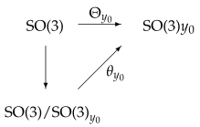
Theorem 4.

Suppose that the stabilizer $\mathsf{SO}{\left(3\right)}_{y_0}$ is homeomorphic to a subgroup of SO(3) generated by the group SO(2). Then, the orbit $\mathsf{SO}\left(3\right)y_0$ is homeomorphic with the sphere $S^2$.

Proof.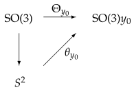 

SO(3) has the structure of a principal SO(2)-bundle over the sphere $S^2$, with the principal bundle projection $\chi :\mathsf{S}\mathsf{O}\left(3\right)\to S^2$ (Theorem 2). If by assumption $\mathsf{SO}{\left(3\right)}_{y_0}=\mathsf{\Sigma }$ is a subgroup of type (b) in the list given by Remark 4, then $\mathsf{S}\mathsf{O}\left(3\right)/\mathsf{\Sigma }=S^2$ and diagram (25) becomes

as required. □

Theorem 5.

Let $(\tau ,y)\to \tau ·y$ be a left action of the special orthogonal group $\mathsf{SO}\left(3\right)$ on a topological space Y. Suppose that for every point $y_0\in Y$ the orbit stabilizer $\mathsf{SO}{\left(3\right)}_{y_0}$ is a connected subgroup of $\mathsf{SO}\left(3\right)$ different from $\mathsf{SO}\left(3\right)$. Then, $\mathsf{SO}{\left(3\right)}_{y_0}$ is isomorphic with $\mathsf{SO}\left(2\right)$ and the orbit $\mathsf{SO}\left(3\right)y_0$ is isomorphic to the sphere $S^2$.

Proof. 

Theorem 5 is an immediate consequence of Theorems 4 and 3. □

6. Smooth Structure of SO(3)

To complete the discussion of the topological structure of SO(3), we prove the existence of a smooth atlas on SO(3), turning the set SO(3) into a smooth manifold of dimension 3. Our aim is to introduce an atlas consisting of a minimum number of charts, called a minimal atlas. This number is determined by the Lusternik–Schnirelmann category  cat X of a manifold X [11]. This topological invariant of a given manifold X is defined as the minimum number n such that there is a covering of X by n open sets, each of which can be contracted to a point inside X. Since $\mathrm{cat}\mathsf{S}\mathsf{O}\left(3\right)=4$ (see [8]), a minimal atlas on SO(3) consists of four charts.

The construction of a minimal atlas of SO(3) is analogous to the construction of a minimal atlas on the unit sphere $S^2$. The fact $\mathrm{cat}{S}^2=2$ gives us that a minimal atlas on $S^2$ consists of two charts. For such construction, the spherical coordinates, or the stereographic projections from two poles, can be employed.

In this paper, by a chart on a topological n-manifold X we mean a pair $(U,\phi )$, where U is an open subset of X, and $\phi :U\to \tilde{U}$ is a homeomorphism of U and an open ball $\tilde{U}$ in ${\mathbf{R}}^n$ (compare with [8]). Two charts, $(U,\mathsf{\Phi })$ and $(\overline{U},\overline{\mathsf{\Phi }})$, are said to be smoothly compatible if either $U\cap \overline{U}=\varnothing$ or the map $\overline{\mathsf{\Phi }}\circ {\mathsf{\Phi }}^{-1}:\mathsf{\Phi }(U\cap \overline{U})\to \overline{\mathsf{\Phi }}(U\cap \overline{U})$ is a diffeomorphism. A smooth atlas for X is a collection of charts whose domains cover X and each pair of the charts is smoothly compatible.

To introduce a smooth atlas on SO(3) explicitly, we use the decomposition of $\tau$ (7) given by Lemma 6. If $-1<z_1<1$, then

$$\left(\begin{array}{ccc}{x}_1& x_2& x_3\\ y_1& y_2& y_3\\ z_1& z_2& z_3\end{array}\right)=\left(\begin{array}{ccc}{x}_1& -{\displaystyle \frac{y_1}{\sqrt{1-z_1^2}}}& -{\displaystyle \frac{x_1{z}_1}{\sqrt{1-z_1^2}}}\\ y_1& {\displaystyle \frac{x_1}{\sqrt{1-z_1^2}}}& -{\displaystyle \frac{y_1{z}_1}{\sqrt{1-z_1^2}}}\\ z_1& 0& \sqrt{1-z_1^2}\end{array}\right)\left(\begin{array}{ccc}1& 0& 0\\ 0& {\displaystyle \frac{z_3}{\sqrt{1-z_1^2}}}& -{\displaystyle \frac{z_2}{\sqrt{1-z_1^2}}}\\ 0& {\displaystyle \frac{z_2}{\sqrt{1-z_1^2}}}& {\displaystyle \frac{z_3}{\sqrt{1-z_1^2}}}\end{array}\right).$$

(26)

Note that $\tau$ and the first factor of the decomposition (26) have the same first column $(x_1,y_1,z_1)$, which can be identified with an element of $S^2$. Using the first chart on $S^2$ (see, e.g., [10]), we have

$$x_1=cos\phi sin\vartheta ,y_1=sin\phi sin\vartheta ,z_1=cos\vartheta ,$$

where $\phi \in (0,2\pi )$, $\vartheta \in (0,\pi )$.

Second factor of the decomposition (26) can be interpreted as an element of SO(2). So, we can assign $\eta \in \mathbf{R}$ to this element such that

$$cos\eta ={\displaystyle \frac{z_3}{\sqrt{1-z_1^2}}},sin\eta ={\displaystyle \frac{z_2}{\sqrt{1-z_1^2}}}.$$

Then,

$$\sqrt{1-z_1^2}=\sqrt{1-{cos}^2\vartheta }=sin\vartheta ,$$

$$z_2=sin\eta \sqrt{1-z_1^2}=sin\vartheta sin\eta ,z_3=cos\eta \sqrt{1-z_1^2}=sin\vartheta cos\eta ,$$

and $\tau$ is uniquely determined by its first column $(x_1,y_1,z_1)$ and its third row $(z_1,z_2,z_3)$. Indeed, from (26), we have

$$\begin{array}{c}{\displaystyle x_2=\frac{-y_1{z}_3-x_1{z}_1{z}_2}{1-z_1^2}=\cdots =-sin\phi cos\eta -cos\phi cos\vartheta sin\eta ,}\hfill \\ {\displaystyle x_3=\frac{y_1{z}_2-x_1{z}_1{z}_3}{1-z_1^2}=\cdots =sin\phi sin\eta -cos\phi cos\vartheta cos\eta ,}\hfill \\ {\displaystyle y_2=\frac{x_1{z}_3-y_1{z}_1{z}_2}{1-z_1^2}=\cdots =cos\phi cos\eta -sin\phi cos\vartheta sin\eta ,}\hfill \\ {\displaystyle y_3=\frac{-x_1{z}_2-y_1{z}_1{z}_3}{1-z_1^2}=\cdots =-cos\phi sin\eta -sin\phi cos\vartheta cos\eta .}\hfill \end{array}$$

So, there is a correspondence between the triples $(\phi ,\vartheta ,\eta )$ and the matrices $\tau \in \mathsf{S}\mathsf{O}\left(3\right)$ in the form

$$\begin{array}{c}\left(\begin{array}{ccc}cos\phi sin\vartheta & -sin\phi cos\eta -cos\phi cos\vartheta sin\eta & sin\phi sin\eta -cos\phi cos\vartheta cos\eta \\ sin\phi sin\vartheta & cos\phi cos\eta -sin\phi cos\vartheta sin\eta & -cos\phi sin\eta -sin\phi cos\vartheta cos\eta \\ cos\vartheta & sin\vartheta sin\eta & sin\vartheta cos\eta \end{array}\right),\hfill \end{array}$$

(27)

which can be considered as the mapping $\mathsf{\Psi }:{\mathbf{R}}^3\to \mathsf{SO}\left(3\right)$, $(\phi ,\vartheta ,\eta )\to \tau$.

Lemma 11.

Let $\tau \in \mathsf{SO}\left(3\right)$ be expressed by (7). If $-1<z_1<1$, then there exists a unique triple $(\phi ,\vartheta ,\eta )\in [0,2\pi )\times \left(0,\pi \right)\times [0,2\pi )$ such that $\mathsf{\Psi }(\phi ,\vartheta ,\eta )=\tau$.

Proof. 

Let us consider $\tau \in \mathsf{S}\mathsf{O}\left(3\right)$ such that $-1<z_1<1$. From (27), there is unique $\vartheta =arccos{z}_1\in \left(0,\pi \right)$. For such $\vartheta$, $sin\vartheta =\sqrt{1-z_1^2}>0$. Again, from (27) we have

$$\begin{array}{c}{\displaystyle sin\eta =\frac{z_2}{\sqrt{1-z_1^2}},cos\eta =\frac{z_3}{\sqrt{1-z_1^2}},}\hfill \\ {\displaystyle sin\phi =\frac{y_1}{\sqrt{1-z_1^2}},cos\phi =\frac{x_1}{\sqrt{1-z_1^2}},}\hfill \end{array}$$

(28)

and there exist unique $\eta \in [0,2\pi )$ and unique $\phi \in [0,2\pi )$ satisfying (28). □

Remark 5.

Lemma 11 is valid when the interval $[0,2\pi )$ is replaced by any interval $[p,q)$ of length $2\pi$.

Let us denote $W=(0,2\pi )\times \left(0,\pi \right)\times (0,2\pi )$. From Lemma 11, the mapping ${\mathsf{\Psi }}_1$ is injective and continuous. Denoting $U_1={\mathsf{\Psi }}_1\left(W\right)$, the inverse of ${\mathsf{\Psi }}_1$ is the mapping ${\mathsf{\Phi }}_1:U_1\to W$,

$$U_1\ni \tau =\left(\begin{array}{ccc}{x}_1& x_2& x_3\\ y_1& y_2& y_3\\ z_1& z_2& z_3\end{array}\right)\to ({\phi }_1,{\vartheta }_1,{\eta }_1)\in W,$$

given by

$$\begin{array}{c}{\displaystyle {\phi }_1=\left\{\begin{array}{cc}{\displaystyle arccos\frac{x_1}{\sqrt{1-z_1^2}},}\hfill & y_1\ge 0,\hfill \\ {\displaystyle 2\pi -arccos\frac{x_1}{\sqrt{1-z_1^2}},}\hfill & y_1<0,\hfill \end{array}\right.}\hfill \\ {\vartheta }_1=arccos{z}_1,\hfill \\ {\displaystyle {\eta }_1=\left\{\begin{array}{cc}{\displaystyle arccos\frac{z_3}{\sqrt{1-z_1^2}},}\hfill & z_2\ge 0,\hfill \\ {\displaystyle 2\pi -arccos\frac{z_3}{\sqrt{1-z_1^2}},}\hfill & z_2<0,\hfill \end{array}\right.}\hfill \end{array}$$

${\mathsf{\Phi }}_1$ is continuous. Thus, ${\mathsf{\Phi }}_1$ is a homeomorphism, and we have completed the proof.

Lemma 12.

The pair $(U_1,{\mathsf{\Phi }}_1)$, ${\mathsf{\Phi }}_1=({\phi }_1,{\vartheta }_1,{\eta }_1)$, is a chart on $\mathsf{SO}\left(3\right)$.

Next, we introduce the mapping ${\mathsf{\Psi }}_2$ on W defined by

$${\mathsf{\Psi }}_2(\phi ,\vartheta ,\eta )=\mathsf{\Psi }(\phi ,\vartheta ,\eta -\pi ).$$

Since $\mathsf{\Psi }$ restricted to the set $(0,2\pi )\times (0,\pi )\times (-\pi ,\pi )$ is injective and continuous, ${\mathsf{\Psi }}_2$ is also injective and continuous. Denoting $U_2={\mathsf{\Psi }}_2\left(W\right)$, the mapping ${\mathsf{\Phi }}_2:U_2\to W$, $\tau \to ({\phi }_2,{\vartheta }_2,{\eta }_2)$, is the inverse of ${\mathsf{\Psi }}_2$ given by

$$\begin{array}{c}{\displaystyle {\phi }_2=\left\{\begin{array}{cc}{\displaystyle arccos\frac{x_1}{\sqrt{1-z_1^2}},}\hfill & y_1\ge 0,\hfill \\ {\displaystyle 2\pi -arccos\frac{x_1}{\sqrt{1-z_1^2}},}\hfill & y_1<0,\hfill \end{array}\right.}\hfill \\ {\vartheta }_2=arccos{z}_1,\hfill \\ {\displaystyle {\eta }_2=\left\{\begin{array}{cc}{\displaystyle \pi +arccos\frac{z_3}{\sqrt{1-z_1^2}},}\hfill & z_2\ge 0,\hfill \\ {\displaystyle \pi -arccos\frac{z_3}{\sqrt{1-z_1^2}},}\hfill & z_2<0,\hfill \end{array}\right.}\hfill \end{array}$$

Lemma 13.

The pair $(U_2,{\mathsf{\Phi }}_2)$, ${\mathsf{\Phi }}_2=({\phi }_2,{\vartheta }_2,{\eta }_2)$, is a chart on $\mathsf{SO}\left(3\right)$. Charts $(U_1,{\mathsf{\Phi }}_1)$ and $(U_2,{\mathsf{\Phi }}_2)$ are smoothly compatible.

Proof. 

Since ${\mathsf{\Phi }}_2$ is continuous, ${\mathsf{\Phi }}_2$ is a homeomorphism.

Coordinate transformation ${\mathsf{\Phi }}_{21}\equiv {\mathsf{\Phi }}_2\circ {\mathsf{\Phi }}_1^{-1}:{\mathsf{\Phi }}_1(U_1\cap U_2)\to {\mathsf{\Phi }}_2(U_1\cap U_2)$ is given by

$${\displaystyle {\phi }_2={\phi }_1,{\vartheta }_2={\vartheta }_1,{\eta }_2=\left\{\begin{array}{cc}\hfill {\displaystyle {\eta }_1+\pi ,}& {\eta }_1\in (0,\pi ),\hfill \\ \hfill {\displaystyle {\eta }_1-\pi ,}& {\eta }_1\in (\pi ,2\pi ).\hfill \end{array}\right.}$$

Analogously, coordinate transformation ${\mathsf{\Phi }}_{12}\equiv {\mathsf{\Phi }}_1\circ {\mathsf{\Phi }}_2^{-1}:{\mathsf{\Phi }}_2(U_1\cap U_2)\to {\mathsf{\Phi }}_1(U_1\cap U_2)$ is given by

$${\displaystyle {\phi }_1={\phi }_2,{\vartheta }_1={\vartheta }_2,{\eta }_1=\left\{\begin{array}{cc}\hfill {\displaystyle {\eta }_2+\pi ,}& {\eta }_1\in (0,\pi ),\hfill \\ \hfill {\displaystyle {\eta }_2-\pi ,}& {\eta }_1\in (\pi ,2\pi ).\hfill \end{array}\right.}$$

Obviously, first partial derivatives of ${\mathsf{\Phi }}_{21}$ and ${\mathsf{\Phi }}_{12}$ are constant; ${\mathsf{\Phi }}_{21}$ and ${\mathsf{\Phi }}_{12}$ are diffeomorphisms on ${\mathsf{\Phi }}_1(U_1\cap U_2)$ and ${\mathsf{\Phi }}_2(U_1\cap U_2)$, respectively, and ${\mathsf{\Phi }}_1(U_1\cap U_2)={\mathsf{\Phi }}_2(U_1\cap U_2)=(0,2\pi )\times \left(0,\pi \right)\times \left((0,\pi )\cup (\pi ,2\pi )\right)$. □

If $-1<y_1<1$, by Lemma 6 we have

$$\left(\begin{array}{ccc}{x}_1& x_2& x_3\\ y_1& y_2& y_3\\ z_1& z_2& z_3\end{array}\right)=\left(\begin{array}{ccc}{x}_1& {\displaystyle \frac{z_1}{\sqrt{1-y_1^2}}}& -{\displaystyle \frac{x_1{y}_1}{\sqrt{1-y_1^2}}}\\ y_1& 0& \sqrt{1-y_1^2}\\ z_1& -{\displaystyle \frac{x_1}{\sqrt{1-y_1^2}}}& -{\displaystyle \frac{y_1{z}_1}{\sqrt{1-y_1^2}}}\end{array}\right)\left(\begin{array}{ccc}1& 0& 0\\ 0& {\displaystyle \frac{y_3}{\sqrt{1-y_1^2}}}& -{\displaystyle \frac{y_2}{\sqrt{1-y_1^2}}}\\ 0& {\displaystyle \frac{y_2}{\sqrt{1-y_1^2}}}& {\displaystyle \frac{y_3}{\sqrt{1-y_1^2}}}\end{array}\right).$$

(29)

Using the second chart on $S^2$ (see, e.g., [10]), we have

$$x_1=-cos\overline{\phi }sin\overline{\vartheta },y_1=-cos\overline{\vartheta },z_1=-sin\overline{\phi }sin\overline{\vartheta },$$

(30)

where $\overline{\phi }\in (0,2\pi )$, $\overline{\vartheta }\in (0,\pi )$.

The second factor of the decomposition (29) can be interpreted as an element of SO(2). So, we can assign $\overline{\eta }\in \mathbf{R}$ to this element such that

$$cos\overline{\eta }={\displaystyle \frac{y_3}{\sqrt{1-y_1^2}}},sin\overline{\eta }={\displaystyle \frac{y_2}{\sqrt{1-y_1^2}}}.$$

Then,

$$\sqrt{1-y_1^2}=\sqrt{1-{cos}^2\overline{\vartheta }}=sin\overline{\vartheta },$$

$$y_2=sin\overline{\eta }\sqrt{1-y_1^2}=sin\overline{\eta }sin\overline{\vartheta },y_3=cos\overline{\eta }\sqrt{1-y_1^2}=cos\overline{\eta }sin\overline{\vartheta },$$

and $\tau$ is uniquely determined by its first column $(x_1,y_1,z_1)$ and second row $(y_1,y_2,y_3)$. Indeed, from (29), we have

$$\begin{array}{c}{\displaystyle x_2=\frac{z_1{z}_3-x_1{y}_1{y}_2}{1-y_1^2}=\cdots =-sin\overline{\phi }cos\overline{\eta }-cos\overline{\phi }cos\overline{\vartheta }sin\overline{\eta },}\hfill \\ {\displaystyle x_3=\frac{-z_1{y}_2-x_1{y}_1{y}_3}{1-y_1^2}=\cdots =sin\overline{\phi }sin\overline{\eta }-cos\overline{\phi }cos\overline{\vartheta }cos\overline{\eta },}\hfill \\ {\displaystyle z_2=\frac{-x_1{y}_3-y_1{y}_2{z}_1}{1-y_1^2}=\cdots =cos\overline{\phi }cos\overline{\eta }-sin\overline{\phi }cos\overline{\vartheta }sin\overline{\eta },}\hfill \\ {\displaystyle z_3=\frac{x_1{y}_2-y_1{y}_3{z}_1}{1-y_1^2}=\cdots =-cos\overline{\phi }sin\overline{\eta }-sin\overline{\phi }cos\overline{\vartheta }cos\overline{\eta }.}\hfill \end{array}$$

So, there is a correspondence between the triples $(\overline{\phi },\overline{\vartheta },\overline{\eta })$ and the matrices $\tau \in \mathsf{S}\mathsf{O}\left(3\right)$ in the form

$$\begin{array}{c}\left(\begin{array}{ccc}-cos\overline{\phi }sin\overline{\vartheta }& -sin\overline{\phi }cos\overline{\eta }-cos\overline{\phi }cos\overline{\vartheta }sin\overline{\eta }& sin\overline{\phi }sin\overline{\eta }-cos\overline{\phi }cos\overline{\vartheta }cos\overline{\eta }\\ -cos\overline{\vartheta }& sin\overline{\vartheta }sin\overline{\eta }& cos\overline{\eta }sin\overline{\vartheta }\\ -sin\overline{\phi }sin\overline{\vartheta }& cos\overline{\phi }cos\overline{\eta }-sin\overline{\phi }cos\overline{\vartheta }sin\overline{\eta }& -cos\overline{\phi }sin\overline{\eta }-sin\overline{\phi }cos\overline{\vartheta }cos\overline{\eta }\end{array}\right),\hfill \end{array}$$

(31)

which can be considered as the mapping $\overline{\mathsf{\Psi }}:{\mathbf{R}}^3\to \mathsf{SO}\left(3\right)$, $(\overline{\phi },\overline{\vartheta },\overline{\eta })\to \tau$.

Lemma 14.

Let $\tau \in \mathsf{SO}\left(3\right)$ be expressed by (7). If $-1<y_1<1$, then there exists a unique triple $(\overline{\phi },\overline{\vartheta },\overline{\eta })\in [0,2\pi )\times \left(0,\pi \right)\times [0,2\pi )$ such that $\overline{\mathsf{\Psi }}(\overline{\phi },\overline{\vartheta },\overline{\eta })=\tau$.

Proof. 

Let us consider $\tau \in \mathsf{S}\mathsf{O}\left(3\right)$ such that $-1<y_1<1$. From (31), there is unique $\overline{\vartheta }=arccos(-y_1)\in \left(0,\pi \right)$. For such $\overline{\vartheta }$, $sin\overline{\vartheta }=\sqrt{1-y_1^2}>0$. Again, from (31), we have

$$\begin{array}{c}{\displaystyle sin\overline{\eta }=\frac{y_2}{\sqrt{1-y_1^2}},cos\overline{\eta }=\frac{y_3}{\sqrt{1-y_1^2}},}\hfill \\ {\displaystyle sin\overline{\phi }=\frac{-z_1}{\sqrt{1-y_1^2}},cos\overline{\phi }=\frac{-x_1}{\sqrt{1-y_1^2}},}\hfill \end{array}$$

and there exist unique $\overline{\eta }\in [0,2\pi )$ and unique $\overline{\phi }\in [0,2\pi )$ satisfying (28). □

Remark 6.

Lemma 14 is valid when the interval $[0,2\pi )$ is replaced by any interval $[p,q)$ of length $2\pi$.

Let us denote ${\mathsf{\Psi }}_3=\overline{\mathsf{\Psi }}{|}_W$. From Lemma 14, the mapping ${\mathsf{\Psi }}_3$ is injective and continuous. Denoting $U_3={\mathsf{\Psi }}_3\left(W\right)$, the inverse of ${\mathsf{\Psi }}_3$ is the mapping ${\mathsf{\Phi }}_3:U_3\to W$,

$$U_3\ni \tau =\left(\begin{array}{ccc}{x}_1& x_2& x_3\\ y_1& y_2& y_3\\ z_1& z_2& z_3\end{array}\right)\to ({\phi }_3,{\vartheta }_3,{\eta }_3)\in W,$$

given by

$$\begin{array}{c}{\displaystyle {\phi }_3=\left\{\begin{array}{cc}{\displaystyle arccos\frac{-x_1}{\sqrt{1-y_1^2}},}\hfill & z_1\le 0,\hfill \\ {\displaystyle 2\pi -arccos\frac{-x_1}{\sqrt{1-y_1^2}},}\hfill & z_1>0,\hfill \end{array}\right.}\hfill \\ {\vartheta }_3=arccos(-y_1),\hfill \\ {\displaystyle {\eta }_3=\left\{\begin{array}{cc}{\displaystyle arccos\frac{y_3}{\sqrt{1-y_1^2}},}\hfill & y_2\ge 0,\hfill \\ {\displaystyle 2\pi -arccos\frac{y_3}{\sqrt{1-y_1^2}},}\hfill & y_2<0,\hfill \end{array}\right.}\hfill \end{array}$$

(32)

Lemma 15.

The pair $(U_3,{\mathsf{\Phi }}_3)$, ${\mathsf{\Phi }}_3=({\phi }_3,{\vartheta }_3,{\eta }_3)$, is a chart on $\mathsf{SO}\left(3\right)$.

Proof. 

${\mathsf{\Phi }}_3$ is continuous; thus, it is a homeomorphism on an open subset of ${\mathbf{R}}^3$. □

Now, we introduce the mapping ${\mathsf{\Psi }}_4$ on W defined by

$${\mathsf{\Psi }}_4(\overline{\phi },\overline{\vartheta },\overline{\eta })=\overline{\mathsf{\Psi }}(\overline{\phi },\overline{\vartheta },\overline{\eta }-\pi ).$$

Since $\overline{\mathsf{\Psi }}$ restricted to the set $(0,2\pi )\times (0,\pi )\times (-\pi ,\pi )$ is injective and continuous, ${\mathsf{\Psi }}_4$ is also injective and continuous. Denoting $U_4={\mathsf{\Psi }}_4\left(W\right)$, the mapping ${\mathsf{\Phi }}_4:U_4\to W$, $\tau \to ({\phi }_4,{\vartheta }_4,{\eta }_4)$, is the inverse of ${\mathsf{\Psi }}_4$ given by

$$\begin{array}{c}{\displaystyle {\phi }_4=\left\{\begin{array}{cc}{\displaystyle arccos\frac{-x_1}{\sqrt{1-y_1^2}},}\hfill & z_1\le 0,\hfill \\ {\displaystyle 2\pi -arccos\frac{-x_1}{\sqrt{1-y_1^2}},}\hfill & z_1>0,\hfill \end{array}\right.}\hfill \\ {\vartheta }_4=arccos(-y_1),\hfill \\ {\displaystyle {\eta }_4=\left\{\begin{array}{cc}{\displaystyle \pi +arccos\frac{y_3}{\sqrt{1-y_1^2}},}\hfill & y_2\le 0,\hfill \\ {\displaystyle \pi -arccos\frac{y_3}{\sqrt{1-y_1^2}},}\hfill & y_2<0,\hfill \end{array}\right.}\hfill \end{array}$$

Lemma 16.

The pair $(U_4,{\mathsf{\Phi }}_4)$, ${\mathsf{\Phi }}_4=({\phi }_4,{\vartheta }_4,{\eta }_4)$, is a chart on $\mathsf{SO}\left(3\right)$. Charts $(U_3,{\mathsf{\Phi }}_3)$, $(U_4,{\mathsf{\Phi }}_4)$ are smoothly compatible.

Proof. 

Analogous to the proof of Lemma 13. □

From the definition of $U_1$, $U_2$, $U_3$ and $U_4$ we obtain their explicit description,

$$\begin{array}{c}{U}_1=\mathsf{S}\mathsf{O}\left(3\right)\setminus \left(\{\tau \in \mathsf{S}\mathsf{O}\left(3\right)\mid x_1\ge 0,y_1=0\}\cup \{\tau \in \mathsf{S}\mathsf{O}\left(3\right)\mid z_3\ge 0,z_2=0\}\right),\hfill \\ U_2=\mathsf{S}\mathsf{O}\left(3\right)\setminus \left(\{\tau \in \mathsf{S}\mathsf{O}\left(3\right)\mid x_1\ge 0,y_1=0\}\cup \{\tau \in \mathsf{S}\mathsf{O}\left(3\right)\mid z_3\le 0,z_2=0\}\right),\hfill \\ U_3=\mathsf{S}\mathsf{O}\left(3\right)\setminus \left(\{\tau \in \mathsf{S}\mathsf{O}\left(3\right)\mid x_1\le 0,z_1=0\}\cup \{\tau \in \mathsf{S}\mathsf{O}\left(3\right)\mid y_3\ge 0,y_2=0\}\right),\hfill \\ U_4=\mathsf{S}\mathsf{O}\left(3\right)\setminus \left(\{\tau \in \mathsf{S}\mathsf{O}\left(3\right)\mid x_1\le 0,z_1=0\}\cup \{\tau \in \mathsf{S}\mathsf{O}\left(3\right)\mid y_3\le 0,y_2=0\}\right).\hfill \end{array}$$

Lemma 17.

The sets $U_1,U_2,U_3,U_4$ cover SO(3).

Proof. 

Denoting

$$\begin{array}{c}{A}_1=\{\tau \in \mathsf{S}\mathsf{O}\left(3\right)\mid x_1\ge 0,y_1=0\},\hfill \\ A_2=\{\tau \in \mathsf{S}\mathsf{O}\left(3\right)\mid x_1\le 0,z_1=0\},\hfill \\ B_1=\{\tau \in \mathsf{S}\mathsf{O}\left(3\right)\mid z_3\ge 0,z_2=0\},\hfill \\ B_2=\{\tau \in \mathsf{S}\mathsf{O}\left(3\right)\mid z_3\le 0,z_2=0\},\hfill \\ C_1=\{\tau \in \mathsf{S}\mathsf{O}\left(3\right)\mid y_3\ge 0,y_2=0\},\hfill \\ C_2=\{\tau \in \mathsf{S}\mathsf{O}\left(3\right)\mid y_3\le 0,y_2=0\},\hfill \end{array}$$

we get

$$\begin{array}{cc}{U}_1=\mathsf{S}\mathsf{O}\left(3\right)\setminus \left(A_1\cup B_1\right),\hfill & U_2=\mathsf{S}\mathsf{O}\left(3\right)\setminus \left(A_1\cup B_2\right),\hfill \\ U_3=\mathsf{S}\mathsf{O}\left(3\right)\setminus \left(A_2\cup C_1\right),\hfill & U_4=\mathsf{S}\mathsf{O}\left(3\right)\setminus \left(A_2\cup C_2\right).\hfill \end{array}$$

Since any matrix $\tau \in \mathsf{S}\mathsf{O}\left(3\right)$ does not have the column consisting of all zeros, we get $A_1\cap A_2=\varnothing$. Also, the pairs of conditions $y_1=0$, $y_1=\pm 1$ and $z_1=0$, $z_1=\pm 1$ cannot be fulfilled simultaneously, so $A_1\cap C_1\cap C_2=\varnothing$ and $A_2\cap B_1\cap B_2=\varnothing$, respectively. Finally $B_1\cap B_2\cap C_1\cap C_2=\varnothing$ because it is impossible to have $y_1=\pm 1$ and $z_1=\pm 1$ for any matrix $\tau \in \mathsf{S}\mathsf{O}\left(3\right)$. Thus, a complement of the union $U_1\cup U_2\cup U_3\cup U_4$ in SO(3) is an empty set. □

Theorem 6.

The charts $(U_1,{\mathsf{\Phi }}_1)$, $(U_2,{\mathsf{\Phi }}_2)$, $(U_3,{\mathsf{\Phi }}_3)$ and $(U_4,{\mathsf{\Phi }}_4)$ represent a smooth atlas on SO(3).

Proof. 

According to Lemma 17, $U_1\cup U_2\cup U_3\cup U_4=\mathsf{>S}\mathsf{O}\left(3\right)$. It should be shown that each pair of these charts is smoothly compatible. In Lemmas 13 and 16, it is shown that the pairs $(U_1,{\mathsf{\Phi }}_1)$, $(U_2,{\mathsf{\Phi }}_2)$ and $(U_3,{\mathsf{\Phi }}_3)$, $(U_4,{\mathsf{\Phi }}_4)$, respectively, are smoothly compatible charts.

Now, let us consider the mapping ${\mathsf{\Phi }}_{31}\equiv {\mathsf{\Phi }}_3\circ {\mathsf{\Phi }}_1^{-1}:{\mathsf{\Phi }}_1(U_1\cap U_3)\to {\mathsf{\Phi }}_3(U_1\cap U_3)$. As a composition of homeomorphisms, ${\mathsf{\Phi }}_{31}$ is also a homeomorphism; its inversion is ${\mathsf{\Phi }}_{13}\equiv {\mathsf{\Phi }}_1\circ {\mathsf{\Phi }}_3^{-1}$.

We have to show that the mapping ${\mathsf{\Phi }}_{31}$ and its inversion ${\mathsf{\Phi }}_{13}$ are $C^{\infty }$. Concrete calculations are omitted. Using (7), (27) and (32), we obtain coordinate expression of ${\mathsf{\Phi }}_{31}$,

$$\begin{array}{c}{\displaystyle {\phi }_3=\left\{\begin{array}{cc}{\displaystyle arccos\frac{-cos{\phi }_{1}sin{\vartheta }_1}{\sqrt{1-{sin}^2{\phi }_1{sin}^2{\vartheta }_1}},}\hfill & \frac{\pi }{2}\le {\vartheta }_1<\pi ,\hfill \\ {\displaystyle 2\pi -arccos\frac{-cos{\phi }_{1}sin{\vartheta }_1}{\sqrt{1-{sin}^2{\phi }_1{sin}^2{\vartheta }_1}},}\hfill & 0<{\vartheta }_1<\frac{\pi }{2},\hfill \end{array}\right.}\hfill \\ {\vartheta }_3=arccos(-sin{\phi }_{1}sin{\vartheta }_1),\hfill \\ {\displaystyle {\eta }_3=\left\{\begin{array}{cc}{\displaystyle arccos\frac{-cos{\phi }_{1}sin{\eta }_1-sin{\phi }_{1}cos{\vartheta }_{1}cos{\eta }_1}{\sqrt{1-{sin}^2{\phi }_1{sin}^2{\vartheta }_1}},}\hfill & \\ cos{\phi }_{1}cos{\eta }_1-sin{\phi }_{1}cos{\vartheta }_{1}sin{\eta }_1\ge 0,\hfill & \\ {\displaystyle 2\pi -arccos\frac{-cos{\phi }_{1}sin{\eta }_1-sin{\phi }_{1}cos{\vartheta }_{1}cos{\eta }_1}{\sqrt{1-{sin}^2{\phi }_1{sin}^2{\vartheta }_1}},}\hfill & \\ cos{\phi }_{1}cos{\eta }_1-sin{\phi }_{1}cos{\vartheta }_{1}sin{\eta }_1<0.\hfill \end{array}\right.}\hfill \end{array}$$

(33)

Let us determine partial derivatives of ${\mathsf{\Phi }}_{31}$. Obviously,

$${\displaystyle \frac{\partial {\phi }_3}{\partial {\eta }_1}}=0,{\displaystyle \frac{\partial {\vartheta }_3}{\partial {\eta }_1}}=0.$$

Moreover,

$$\begin{array}{c}{\displaystyle \frac{\partial }{\partial {\phi }_1}\left(arccos\frac{-cos{\phi }_{1}sin{\vartheta }_1}{\sqrt{1-{sin}^2{\phi }_1{sin}^2{\vartheta }_1}}\right)=\cdots =-\frac{sin{\phi }_{1}sin{\vartheta }_1{cos}^2{\vartheta }_1}{|cos{\vartheta }_1|(1-{sin}^2{\phi }_1{sin}^2{\vartheta }_1)}.}\hfill \end{array}$$

For ${\displaystyle \frac{\pi }{2}}\le {\vartheta }_1<\pi$, we have $|cos{\vartheta }_1|=-cos{\vartheta }_1$, and

$${\displaystyle \frac{\partial {\phi }_3}{\partial {\phi }_1}=-\frac{sin{\phi }_{1}sin{\vartheta }_1{cos}^2{\vartheta }_1}{-cos{\vartheta }_1(1-{sin}^2{\phi }_1{sin}^2{\vartheta }_1)}=\frac{sin{\phi }_{1}sin{\vartheta }_{1}cos{\vartheta }_1}{1-{sin}^2{\phi }_1{sin}^2{\vartheta }_1}.}$$

For $0<{\vartheta }_1<{\displaystyle \frac{\pi }{2}}$, we have $|cos{\vartheta }_1|=cos{\vartheta }_1$, and

$${\displaystyle \frac{\partial {\phi }_3}{\partial {\phi }_1}=\frac{sin{\phi }_{1}sin{\vartheta }_1{cos}^2{\vartheta }_1}{cos{\vartheta }_1(1-{sin}^2{\phi }_1{sin}^2{\vartheta }_1)}=\frac{sin{\phi }_{1}sin{\vartheta }_{1}cos{\vartheta }_1}{1-{sin}^2{\phi }_1{sin}^2{\vartheta }_1},}$$

so finally, on ${\mathsf{\Phi }}_1(U_1\cap U_3)$, we have

$${\displaystyle \frac{\partial {\phi }_3}{\partial {\phi }_1}=\frac{sin{\phi }_{1}sin{\vartheta }_{1}cos{\vartheta }_1}{1-{sin}^2{\phi }_1{sin}^2{\vartheta }_1}.}$$

Analogously, on ${\mathsf{\Phi }}_1(U_1\cap U_3)$ we obtain

$${\displaystyle \frac{\partial {\phi }_3}{\partial {\vartheta }_1}=\frac{-cos{\phi }_1}{1-{sin}^2{\phi }_1{sin}^2{\vartheta }_1},\frac{\partial {\vartheta }_3}{\partial {\phi }_1}=\frac{cos{\phi }_{1}sin{\vartheta }_1}{\sqrt{1-{sin}^2{\phi }_1{sin}^2{\vartheta }_1}},\frac{\partial {\vartheta }_3}{\partial {\vartheta }_1}=\frac{sin{\phi }_{1}cos{\vartheta }_1}{\sqrt{1-{sin}^2{\phi }_1{sin}^2{\vartheta }_1}},}$$

$${\displaystyle \frac{\partial {\eta }_3}{\partial {\phi }_1}=\frac{cos{\vartheta }_1}{1-{sin}^2{\phi }_1{sin}^2{\vartheta }_1},\frac{\partial {\eta }_3}{\partial {\vartheta }_1}=-\frac{sin{\phi }_{1}cos{\phi }_{1}sin{\vartheta }_1}{1-{sin}^2{\phi }_1{sin}^2{\vartheta }_1},\frac{\partial {\eta }_3}{\partial {\eta }_1}=1.}$$

Obviously, all partial derivatives of ${\mathsf{\Phi }}_{31}$ on ${\mathsf{\Phi }}_1(U_1\cap U_3)$ of all orders exist and are continuous; thus, ${\mathsf{\Phi }}_{31}$ is smooth.

Coordinate expression of ${\mathsf{\Phi }}_{13}$ is given by mutual exchange of the indices 1 and 3 in (33). Thus, ${\mathsf{\Phi }}_{13}$ is smooth, which implies that the charts $(U_1,{\mathsf{\Phi }}_1)$ and $(U_3,{\mathsf{\Phi }}_3)$ are smoothly compatible. We have analogous results for other pairs of charts, namely $(U_1,{\mathsf{\Phi }}_1)$ and $(U_4,{\mathsf{\Phi }}_4)$; $(U_2,{\mathsf{\Phi }}_2)$ and $(U_3,{\mathsf{\Phi }}_3)$; $(U_2,{\mathsf{\Phi }}_2)$ and $(U_4,{\mathsf{\Phi }}_4)$. □

Remark 7.

Using parametrizations, Grafarend and Kuhnel in [8] introduced four types of minimal atlases on SO(3), each consisting of four coordinate charts. For example, one of them, the atlas consisting of charts given by Cardan angles, belongs to the same smooth structure on SO(3) as represented by the atlas in Theorem 6.

References

- Krupka, D.; Brajerčík, J. On the Structure of SO(3): Trace and Canonical Decompositions. Mathematics 2024, 12, 1490. [Google Scholar]
- Alperin, J.L.; Bell, R.B. Groups and Representations; Graduate Texts in Mathematics 162; Springer: Berlin/Heidelberg, Germany, 1995. [Google Scholar]
- Dieudonné, J. Treatise on Analysis; Academic Press: Cambridge, MA, USA, 1972; Volume III. [Google Scholar]
- Godbillon, C. Géométrie Différentielle et Mécanique Analytique; Hermann: Paris, France, 1969. [Google Scholar]
- Krupka, D.; Krupková, O. Topology and Geometry; Lectures and Solved Problems; SPN: Praha, Czechia, 1989. (In Czech) [Google Scholar]
- Kurosh, A. Higher Algebra; Mir Publishers: Moscow, Russia, 1980. [Google Scholar]
- Warner, F.W. Foundations of Differentiable Manifolds and Lie Groups; Springer: Berlin/Heidelberg, Germany, 1983. [Google Scholar]
- Grafarend, E.W.; Kuhnel, W. A minimal atlas for the rotation group SO(3). Int. J. Geomath 2011, 2, 113–122. [Google Scholar] [CrossRef]
- Cheraghchi, S.; Voicu, N.; Pfeifer, C. Four-dimensional SO(3)-spherically symmetric Berwald Finsler space. Int. J. Geom. Method Mod. Phys. 2023, 20, 1–23. [Google Scholar] [CrossRef]
- Krupka, D.; Brajerčík, J. Schwarzschild spacetimes: Topology. Axioms 2022, 11, 693. [Google Scholar] [CrossRef]
- Lusternik, L.; Schnirelmann, L. Sur un principe topologique en analyse. C. R. Acad. Sci. Paris 1929, 188, 295–297. [Google Scholar]
Disclaimer/Publisher’s Note: The statements, opinions and data contained in all publications are solely those of the individual author(s) and contributor(s) and not of MDPI and/or the editor(s). MDPI and/or the editor(s) disclaim responsibility for any injury to people or property resulting from any ideas, methods, instructions or products referred to in the content. |
© 2025 by the authors. Licensee MDPI, Basel, Switzerland. This article is an open access article distributed under the terms and conditions of the Creative Commons Attribution (CC BY) license (https://creativecommons.org/licenses/by/4.0/).