Numerical Simulation of the Entrance Length in a Laminar Pipe Flow at Low Reynolds Numbers

Abstract

According to Prandtl’s boundary layer theory, the entrance length refers to the axial distance required for a flow to transition from its initial entry condition to a fully developed flow where the velocity profile stabilizes downstream. However, this theory remains applicable only under the assumption of Re ≫ 1, while its validity diminishes under low-Reynolds-number conditions. This study utilizes OpenFOAM based on the finite volume method to numerically examine Newtonian and viscoelastic fluids in a laminar circular pipe flow. The objective is to determine the range of Reynolds numbers for which the differential equations from within the Prandtl boundary layer theory are strictly valid. Additionally, the study explores the effects of Reynolds numbers (Re) ranging from 50 to 100, s solvent viscosity ratio (β) fixed at 0.3 and 0.7, and Weissenberg numbers (Wi) ranging from 0.2 to 5 on the entrance length and friction factor for the Oldroyd-B model. The results indicate the presence of a lower Reynolds number that impedes the attainment of the outcomes predicted by the Prandtl boundary layer theory for the entrance length. The inertia effect, the increase in solvent viscosity contribution, and the elastic effect exhibit a linear relationship with the entrance length and friction factor.

1. Introduction

Prandtl’s boundary layer theory provided the foundation for subsequent research in this field, with numerous scholars employing it as a foundational principle in their studies, particularly in investigating the entrance length. Prandtl pointed out that fluid flows with a low viscosity can be divided into a boundary layer near solid surfaces and interfaces, patched onto a nearly inviscid outer layer. In a pipe flow, when the boundary layer expands to the centerline of the conduit, the velocity profile ceases to vary along the axial direction, at which point the flow is termed a fully developed flow. The entrance length (L_e) is defined as the distance required for fluid flow to transition from pipe entry flow to a fully developed flow. For laminar flow, Prandtl derived the relationship between entrance length (L_e), Reynolds number (Re), and pipe diameter (D): L_e/D = 0.06 Re.

Determining the entrance length in a pipe is crucial in fluid mechanics and engineering applications. The sufficient straight pipe length must be ensured before using the measuring devices to avoid inaccuracies. Accurate estimation of entrance length is critical for minimizing energy losses in industrial fluid systems. By analyzing entrance effects, engineers can design more reliable, efficient, and cost-effective fluid systems.

Viscoelastic fluids [1] are complex fluids that simultaneously exhibit both viscous dissipation and elastic effects. Stress relaxation occurs over a characteristic relaxation time (λ), quantified by the Weissenberg number (Wi). Viscoelastic fluids exert a profound influence on modern engineering due to their unique rheological properties. The complex behavior of viscoelastic fluids presents significant prediction challenges, leaving many viscoelastic fluids phenomena still undiscovered.

The fluid properties of viscoelastic fluids also significantly influence the entrance length in laminar flow. For the study of entrance length in Newtonian and viscoelastic fluids, numerous researchers have carried out extensive investigations through mathematical theoretical analysis, numerical simulation, and experiments. Langhaar [2] solved the Navier–Stokes equations for laminar flow in a pipe. This solution was obtained by means of a linear approximation method, which determined the relationship between the entrance length and the Reynolds number using the velocity distribution curve. Campbell and Slattery [3] contemplated the effect of viscous dissipation within the boundary layer in the entrance region flow theory. Sparrow et al. [4] employed a theoretical analysis and numerical methods to derive an expression for the velocity distribution in the entrance region of the laminar flow in a pipe. They also discussed the factors affecting the entrance length. Friedmann et al. [5] conducted a study of the entrance length of a homogeneous viscous liquid in a pipe laminar flow within the range of low to medium Reynolds numbers. The flow characteristics, including the velocity distribution of the fluid, were obtained through the implementation of the numerical finite difference method and subsequently analyzed for working conditions in which the Reynolds number approaches zero.

Na and Yoo [6] numerically employed the SIMPLER algorithm in a non-uniform staggered grid system to investigate the developing flow of Oldroyd-B model in the planar entrance region. Alves et al. [7] investigated the flow characteristics of a PTT (Phan-Thien–Tanner) linear viscoelastic fluid in a two-dimensional 4:1 contraction flow, defining the entrance length as an axial location where the axial normal stress drops to 1 or 5% of its maximum value. Durst et al. [8] presented a relationship between the entrance length of a laminar flow pipe and the Reynolds number. They defined the entrance length as the axial location where the centerline velocity reaches 99% of its fully developed value. Poole and Ridley et al. [9] provided the results of a numerical investigation of the pipe flow of inelastic non-Newtonian fluids. They proposed a correlation between the power law exponent (0.4 < n < 1.5) and the entrance length segment in the range 0 < Re < 1000. Yapici et al. [10] employed a finite-volume method to numerically simulate the steady-state flow of Oldroyd-B fluids and PTT-linear fluids in a two-dimensional rectangular channel. The effects of the Weissenberg number (Wi), computational mesh, inlet boundary conditions, and Reynolds number (Re) on the entrance length were investigated. Bertoco et al. [11] investigated the development length in pressure-driven viscoelastic fluid flows between parallel plates, modeled by the gPTT (generalized Phan-Thien–Tanner) constitutive equation. They used the finite-difference method to analyze the effects of model parameters. Mahdavi et al. [12] investigated the fluid properties of nanofluids in the entrance length of laminar flat plate flow. Numerical simulations revealed that the boundary layer immediately started forming at the beginning of the entrance region and merged long before the fully developed section. Furthermore, the location of the merging point is determined only by the Reynolds number. Lavrov [13] investigated the entrance length of Bingham fluid for a laminar flow between parallel flat plates at 0 < Bi < 1000 by means of the momentum integral solution, the Batra–Kandasamy method, and the Gupta method.

Chen [14] used the momentum integral method to analyze laminar Newtonian flow development in the entrance regions of circular pipes and parallel-plate channels at low Reynolds numbers. Everts and Meyer [15] experimentally investigated the hydrodynamic and thermal entrance lengths for laminar Newtonian flow in smooth horizontal tubes under constant heat flux conditions.

However, Prandtl’s boundary layer theory is highly effective under the assumption of a high Reynolds number (Re ≫ 1). The theory is invalid under low-Reynolds-number conditions. It indicates that the effect of the Reynolds number governing the entrance length is only valid within a certain operational range. Previous studies on the entrance length have predominantly focused on CFD simulations of confined channel flow, while research on the characteristics of viscoelastic fluids in circular pipes remains scarce. This study investigates the entrance length of viscoelastic fluids in a laminar pipe flow using OpenFOAM [16] along with the RheoTool [17] package. The Oldroyd-B model, as a simple viscoelastic model, achieves mathematical tractability while maintaining physical objectivity. Numerical simulations of incompressible Newtonian and Oldroyd-B fluids in a laminar pipe flow are realized using the LCR (Log-Conformation Representation) method [18,19] to obtain the flow characteristics of the fluids. Numerous studies have demonstrated the reliability and precision of the LCR method in numerical calculations [20,21,22,23]. This study is conducted on the low Reynolds numbers within the framework of the boundary layer theory for Newtonian fluids, focusing on the factors that affect entrance lengths and friction factors in the Oldroyd-B model. Much consideration is given to the effects of Reynolds numbers (Re) ranging from 50 to 100, a solvent viscosity ratio (β) ranging from 0.3 to 0.7, and Weissenberg numbers (Wi) ranging from 0.2 to 5 on the entrance length and friction factor in the Oldroyd-B model. While simulating high Weissenberg number (Wi ≫ 1) conditions in three-dimensional models presents significant computational challenges, this study provides the entrance length characteristics of viscoelastic fluids under elevated Weissenberg number conditions.

Combined with the above analysis, the main research content of this paper is as follows. Section 2 describes the mathematical model and numerical methods employed to solve the Oldroyd-B model equations. Section 3 presents and discusses the results of the numerical simulations in the Newtonian and Oldroyd-B fluids, and Section 4 provides conclusions and directions for future work on the entrance length.

2. Governing Equations and Methods

2.1. Governing Equations

For a viscoelastic fluid flow, the governing equations consist of the incompressible continuity equation and the momentum equation:

$$\nabla ·\mathit{u}=0$$

(1)

$$\rho \left({\displaystyle \frac{\partial \mathit{u}}{\partial t}}+\mathit{u}·\nabla \mathit{u}\right)=-\nabla p+\nabla ·\mathit{\tau }$$

(2)

where $\mathit{u}$ is the velocity vector, $\rho$ is the density, $p$ is the pressure, $\mathit{\tau }$ is the total stress tensor, which can be decomposed into the solvent $\left({\mathit{\tau }}_s\right)$ and polymer $\left({\mathit{\tau }}_p\right)$ stress tensors, as follows:

$$\mathit{\tau }={\mathit{\tau }}_s+{\mathit{\tau }}_p$$

(3)

In Equation (3), ${\mathit{\tau }}_s$ is given by the Newtonian law ${\mathit{\tau }}_s={\eta }_s\left[\nabla \mathit{u}+{\left(\nabla \mathit{u}\right)}^{\mathbf{T}}\right]$, where ${\eta }_s$ is the solvent viscosity.

The constitutive equation for the Oldroyd-B model [24,25] is of the form

$${\mathit{\tau }}_p+\lambda \stackrel{\nabla }{{\mathit{\tau }}_p}={\eta }_p\left[\nabla \mathit{u}+{\left(\nabla \mathit{u}\right)}^{\mathbf{T}}\right]$$

(4)

where ${\eta }_p$ is the polymer viscosity at the zero-shear rate, $\lambda$ is the relaxation time. $\stackrel{\nabla }{{\mathit{\tau }}_p}$ denotes the upper converted time derivative of ${\mathit{\tau }}_p$, which is defined as

$$\stackrel{\nabla }{{\mathit{\tau }}_p}={\displaystyle \frac{\partial {\mathit{\tau }}_p}{\partial t}}+\mathit{u}·\nabla {\mathit{\tau }}_p-{\mathit{\tau }}_p·\nabla \mathit{u}-{\left(\nabla \mathit{u}\right)}^{\mathbf{T}}·{\mathit{\tau }}_p$$

(5)

The constitutive equation is formulated using the conformation tensor $\mathit{C}$. The polymer stress and the conformation tensor are related to each other by

$${\mathit{\tau }}_p={\displaystyle \frac{{\eta }_p}{\lambda }}\left(\mathit{C}-\mathit{I}\right)$$

(6)

The conformation tensor $\mathit{C}$ can be diagonalized as

$$\mathit{C}=\mathit{R}\mathsf{\Lambda }{\mathit{R}}^{\mathbf{T}}$$

(7)

where $\mathit{R}$ is the eigenvector matrix fulfilling $\mathit{R}{\mathit{R}}^{\mathbf{T}}={\mathit{R}}^{\mathbf{T}}\mathit{R}=\mathit{I}$ and $\mathsf{\Lambda }$ is the diagonal matrix containing the eigenvalues of $\mathit{C}$.

The equation for the conformation tensor in the Oldroyd-B model can be rewritten as

$${\displaystyle \frac{D\mathit{C}}{Dt}}=\mathit{C}\mathit{L}+{\mathit{L}}^{\mathbf{T}}\mathit{C}+{\displaystyle \frac{1}{\lambda }}\left(\mathit{I}-\mathit{C}\right)$$

(8)

where $\mathit{L}=\nabla \mathit{u}$.

Defining $\tilde{\mathsf{\Omega }}={\mathit{R}}^{\mathbf{T}}{\displaystyle \frac{D\mathit{R}}{Dt}}$ and $\tilde{\mathit{L}}={\mathit{R}}^{\mathbf{T}}\mathit{L}\mathit{R}$, Equation (8) can be obtained as

$$\tilde{\mathsf{\Omega }}\mathsf{\Lambda }+{\displaystyle \frac{D\mathsf{\Lambda }}{Dt}}+\mathsf{\Lambda }{\tilde{\mathsf{\Omega }}}^{\mathrm{T}}=\mathsf{\Lambda }\tilde{\mathit{L}}+{\tilde{\mathit{L}}}^{\mathbf{T}}\mathsf{\Lambda }+{\displaystyle \frac{1}{\lambda }}\mathit{I}-{\displaystyle \frac{1}{\lambda }}\mathsf{\Lambda }$$

(9)

The logarithm of $\mathit{C}$ is defined as

$$\mathit{S}=\log \mathit{C}=\mathit{R}\log \mathsf{\Lambda }{\mathit{R}}^{\mathbf{T}}$$

(10)

Equation (9) can be rewritten as

$${\displaystyle \frac{D\mathit{S}}{Dt}}=\mathit{R}\left(\tilde{\mathsf{\Omega }}\log \mathsf{\Lambda }+{\displaystyle \frac{D\mathsf{\Lambda }}{Dt}}{\mathsf{\Lambda }}^{-1}+\log \mathsf{\Lambda }{\tilde{\mathsf{\Omega }}}^{\mathrm{T}}\right){\mathit{R}}^{\mathbf{T}}$$

(11)

The equation for the logarithmic conformation tensor in the Oldroyd-B model can be obtained:

$${\displaystyle \frac{D\mathit{S}}{Dt}}=\mathsf{\Omega }\mathit{S}-\mathit{S}\mathsf{\Omega }+2\mathit{B}+{\displaystyle \frac{1}{\lambda }}\left(e^{-\mathit{S}}-\mathit{I}\right)$$

(12)

where ${\tilde{\mathit{B}}}_{ii}={\tilde{\mathit{L}}}_{ii}$, $\mathit{B}=\mathit{R}\tilde{\mathit{B}}{\mathit{R}}^{\mathbf{T}}$, and $\mathsf{\Omega }=\mathit{R}\tilde{\mathsf{\Omega }}{\mathit{R}}^{\mathbf{T}}$.

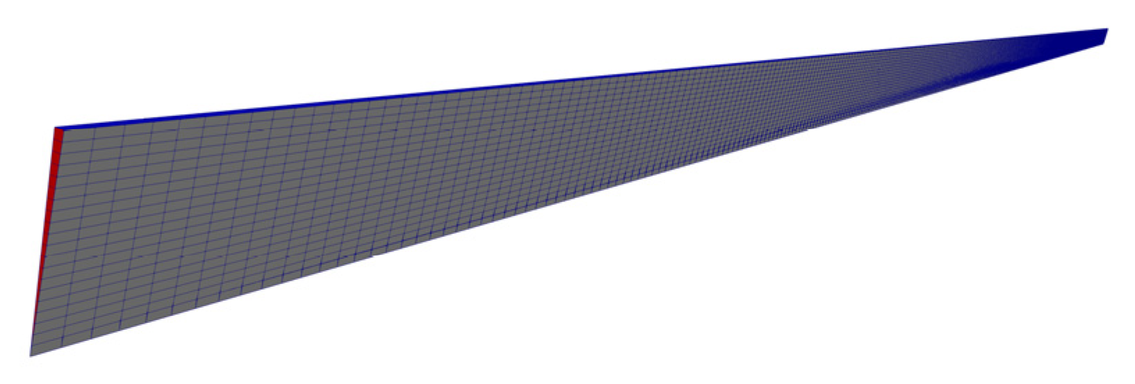
2.2. Geometry and Boundary Conditions

For axi-symmetric cases, the pipe is approximated by a wedge-shaped mesh with a small angle and a thickness of one cell, running along the centerline, straddling one of the coordinate planes, as shown in Figure 1. The axi-symmetric wedge planes must be specified as separate patches with a wedge shape. In this geometry, the x-coordinate represents the pipe axis, and the y-coordinate represents the pipe radius. The wedge boundary type is implemented using a 3D wedge-shaped mesh that mathematically represents axi-symmetric conditions, though it is not strictly a cylindrical-polar structured mesh in the traditional sense. A mesh diagram is shown in Figure 2.

The ratio of pipe length (L) to pipe diameter (D) is 50:1 to ensure fully developed flow conditions. x/D and y/D are the normalized x-coordinate and y-coordinate, respectively, and a uniform mesh is used in this geometry. The inlet is assigned a uniform velocity, the pipe wall is defined as a no-slip boundary condition, the center axis is treated as a symmetry condition, and the outlet is set at zero backpressure.

2.3. Numerical Method

The laminar pipe flow is simulated using OpenFOAM, along with RheoTool package. For non-Newtonian fluids, the polymer stresses undergo a substantial increase, resulting in significant numerical instability during simulations. This study proposes the utilization of the LCR method to enhance the numerical stability of the simulations. In a recent study, Mohanty et al. [26] used the OpenFOAM-based LCR method to investigate the influence of the solvent viscosity ratio and Deborah number on the creeping flow of an Oldroyd-B viscoelastic fluid past a channel-confined cylinder. The solution in this study differs from that of Mohanty’s study mainly in the discretization scheme used for the governing equations and the choice of solver. To enhance the convergence of iterations, a steady solution is achieved by obtaining a long-term solution to an unsteady problem, thereby retaining the time derivatives in the governing equations. The temporal derivative terms are discretized using the implicit Euler scheme. The convective terms in the momentum and constitutive equations are discretized with the CUBISTA (Convergent and Universally Bounded Interpolation Scheme for Treatment of Advection) [27] scheme for discretization, and the coupling of pressure and velocity is performed using the SIMPLE algorithm. Numerical relaxation of the governing equations is mainly used for the field relaxation by introducing relaxation factors to control variable updates. The numerical simulation focuses on field relaxation techniques specifically applied to pressure fields, velocity fields, stress fields, and tensors, and the relaxation factor for these fields is uniformly set to 1.

The pressure and velocity fields are solved using the smooth solver along with the GaussSeidel smoother which is an iterative solver but also as a widely used smoother. Its local error smoothing property makes it effective in eliminating high-frequency errors, particularly in elliptic partial differential equations. It is imperative to ensure that residuals vary smoothly during the solution process in order to enhance numerical stability. The residual dimensionless value of the pressure and velocity fields is 10⁻⁷. The stress field and conformation tensors are solved using the PBiCG (Preconditioned Bi-conjugate Gradient) solver along with the DILU (Diagonal-based Incomplete LU) preconditioner. This solver is utilized for the resolution of asymmetric coefficient matrices, yielding residual dimensionless values of 10⁻⁶.

The dimensionless parameters are defined as follows:

$$Re={\displaystyle \frac{\rho VD}{{\eta }_0}}$$

(13)

where $V$ is the average velocity of the fluid, and ${\eta }_0={\eta }_s+{\eta }_p$ is the solvent and polymer viscosities at the zero-shear rate.

$$Wi={\displaystyle \frac{\lambda V}{D}}$$

(14)

$$\beta ={\displaystyle \frac{{\eta }_s}{{\eta }_0}}$$

(15)

$$h_f={\lambda }_f{\displaystyle \frac{L}{D}}{\displaystyle \frac{V^2}{2g}}={\displaystyle \frac{\mathsf{\Delta }{p}_f}{\rho g}}$$

(16)

where $h_f$ is the friction head loss, ${\lambda }_f$ is the friction factor, $g$ is the gravitational acceleration which is typically taken to be 9.8 m/s², and $\mathsf{\Delta }{p}_f$ is the pressure drop due to fluid resistance.

3. Results

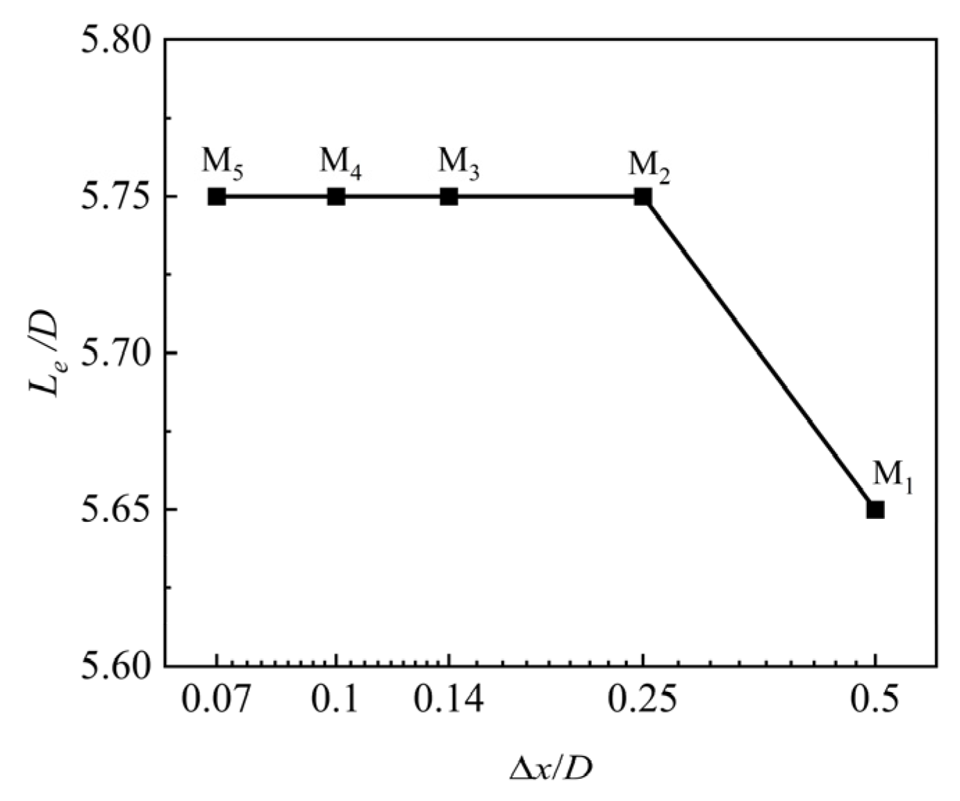
3.1. Grid Independence Verification

To ensure the stability of the computational grid and the accuracy of the present results, mesh independency is demonstrated. Numerical computations are performed using five grid resolutions, with the mesh characteristics tabulated in

Table 1. Characteristics of meshes for pipe flow.

Mesh	Number of Nodes	Δx/D	Δy/D
M1	100 × 5	0.5	0.1
M2	200 × 10	0.25	0.05
M3	350 × 15	0.1429	0.0333
M4	500 × 20	0.1	0.025
M5	700 × 30	0.0714	0.0167

. The numerical results for the entrance length of the Newtonian fluid at Re = 100 are verified using the dimensionless entrance length L_e/D = 0.0575 Re, as defined by Langhaar [2].

As shown in Figure 3, when Δx/D ≤ 0.25, the entrance length of the Newtonian fluid is consistent with Langhaar’s definitions [2] and remains essentially unchanged numerically. The use of 500 × 20 grid as the final computational grid is predicated on the necessity to ensure the stability of the results and calculation speed.

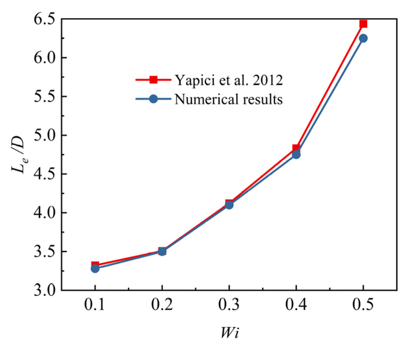
3.2. Accuracy Verification

To validate the LCR method, the results were compared with the entrance lengths of an Oldroyd-B fluid in a two-dimensional rectangular channel at Re = 0.001 and β = 0.1 [10]. The fundamental principles underpinning entrance length studies remain consistent, irrespective of the dimensionality of the geometric model employed. The dimensionality of the geometric model does not engender any difference in their numerical methods. In order to simplify the computational difficulty of reliability validation, the computational model is validated in comparison with that of Yapici et al. [10]. Dimensionless entrance lengths are, respectively, compared at Wi = 0.1–0.5, and the results are shown in Figure 4. The maximum deviation is 2.89%, while the minimum deviation is 0.21%. These findings indicate that both the computational model and process can be considered reliable.

3.3. Lower Reynolds Number

Prandtl’s boundary layer theory states that the viscous properties of fluids exert an influence on the flow within a very small thickness, denoted by δ, near the surface of the object. In the event that the characteristic dimension in the direction of fluid flow is denoted by l, the boundary layer thickness is denoted as ${\displaystyle \frac{\delta }{l}} ~{\displaystyle \frac{1}{\sqrt{{Re}_l}}}$. This theory applies to high-Reynolds-number flows where inertia dominates viscosity. Specifically, Re_l should satisfy Re_l ≫ 1 and δ ≪ l must hold. The hydrodynamic entrance length (L_e) demonstrates a linear proportionality to the Reynolds number (Re), as expressed by the relation L_e/D = C·Re, where C is the dimensionless development coefficient. However, under low-Reynolds-number conditions, the aforementioned theoretical relationship becomes invalid. Therefore, numerical simulations identify the range of Reynolds numbers that satisfy δ/l ≪ 1, ensuring the boundary layer differential equations’ validity.

The laminar flow characteristics of Newtonian fluid were examined in a pipe with different Reynolds numbers. The simulation results for a dimensionless entrance length were compared with L_e/D = 0.0575 Re, as defined by Langhaar [2]. Figure 5 reflects the effect of Re on the dimensionless entrance length of Newtonian fluid. Both simulations and theory show a linear growth of entrance length with increasing Re. For Re ≥ 40, the simulated and theoretical results agree closely. Below Re = 40, the results increasingly deviate from the theory as Re decreases. The deviation grows systematically with decreasing Re, consistently exceeding theoretical predictions. We identified a critical Reynolds number (Re_L = 40) below which Prandtl’s boundary layer conditions fail. This lower boundary, represented by Re_L = 40, signifies the point at which the condition of strict satisfaction is no longer met. Consequently, Prandtl boundary layer differential equations cannot be strictly established.

3.4. Influence of Dimensionless Entrance Length and Friction Factor

3.4.1. Reynolds Number

The Reynolds number directly affects laminar flow fields through inertial forces. We quantify inertia’s effect on entrance length and friction factor across Reynolds numbers. In Figure 6a–c, the dimensionless centerline velocities of the pipe are represented for various Reynolds numbers in the Newtonian and Oldroyd-B fluids with β = 0.5. The centerline velocities increase with x/D for both fluids, with Oldroyd-B showing more pronounced development. Newtonian fluids reach the expected maximum velocity (twice the average velocity), matching the analytical solutions. The Oldroyd-B fluids show a stronger velocity development before reaching a fully developed flow.

We analyzed the inertial effects on entrance lengths for Newtonian and Oldroyd-B fluids at Re = 50, 75, and 100. Figure 7 reveals that the dimensionless entrance length in Oldroyd-B model is found to be particularly influenced by Re. The entrance lengths in Oldroyd-B model grow with Re, consistent with Yapici et al. [10]. The Oldroyd-B model shows significantly longer entrance lengths than the Newtonian fluids. The dependence of entrance length on Re intensifies with higher Weissenberg numbers (Wi). L_e/D in the Oldroyd-B model exhibits minimal Re sensitivity at Wi < 1, but a strong dependence at Wi ≥ 1.

Oldroyd-B fluid’s properties affect both entrance length and friction factor λ_f. Figure 8 reflects λ_f for Newtonian and Oldroyd-B fluids at different Re values with β = 0.5. A close examination reveals that the slopes of curves for the Newtonian and Oldroyd-B fluids are essentially the same. λ_f in the Oldroyd-B model decreases more sharply with Re and remains lower than Newtonian values. At Wi = 0.2, λ_f nearly matches the Newtonian behavior, converging as elasticity decreases.

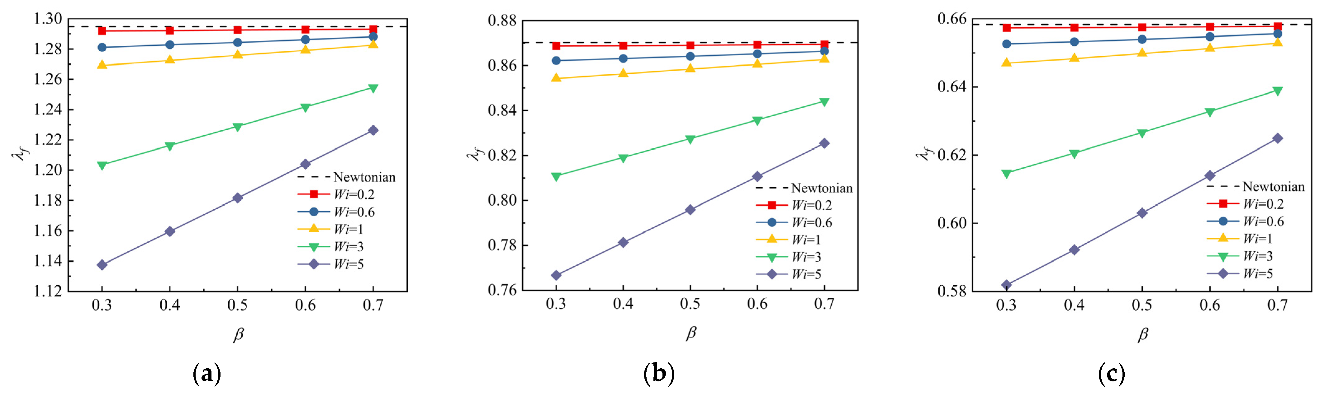
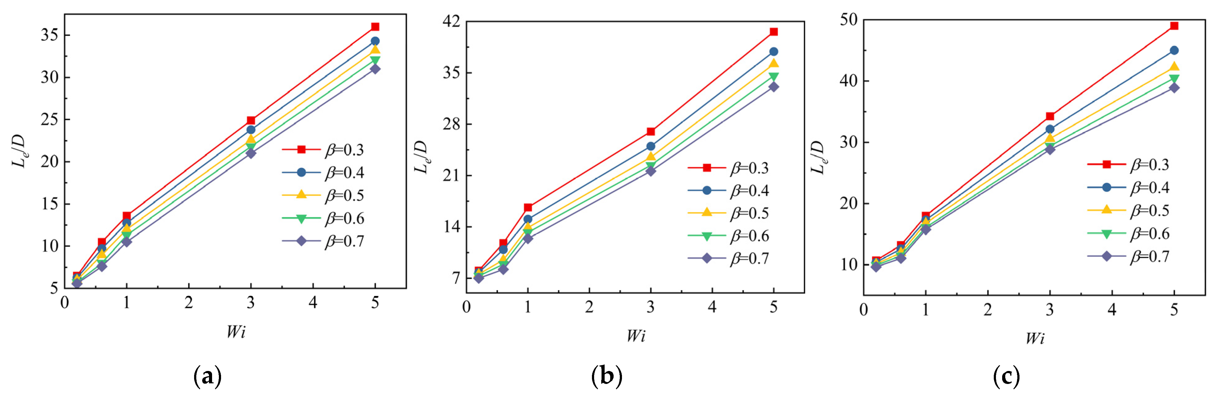
3.4.2. Solvent Viscosity Ratio

The solvent viscosity ratio β has been shown to reflect the contribution of a polymer to solution viscosity. It reveals an inverse relationship between β and the solute’s viscous contribution in the viscoelastic fluid. Figure 9 shows that decreasing β (increasing solute viscosity) augments L_e/D in Oldroyd-B fluids. The slope of the curve increases gradually as the contribution of solute viscosity increases. L_e/D exhibits a smoother curve and greater resistance to variation with β when Wi < 1. Conversely, under conditions of high Wi (Wi ≥ 1), the results are more susceptible to β, and the greater the Wi, the more pronounced the increase in L_e/D.

Additionally, the friction factor is influenced by the solvent viscosity ratio. Figure 10 shows the law of variation in an Oldroyd-B fluid’s λ_f for different β at Re = 50, 75, and 100. λ_f increases with β, but remains nearly constant for Wi = 0.2, matching Newtonian behavior. At Wi ≥ 1, the effect of solvent viscosity ratio intensifies with Wi, producing λ_f values substantially below Newtonian levels.

3.4.3. Weissenberg Numbers

The Weissenberg number is indicative of the extent to which the elastic properties of a fluid predominate during shear or tensile flow. The effect of varying Wi on the entrance length in Oldroyd-B fluid at Re = 50, 75, and 100 is demonstrated in Figure 11. As Wi increases, L_e/D in the Oldroyd-B fluid gradually increases. At Wi < 1, L_e/D changes minimally, especially at Re = 50, while Re = 100 shows dramatic increases. For Wi ≥ 1, L_e/D rises sharply with Wi, particularly at Re = 100, while Wi = 5 produces extreme elongation.

Figure 12 presents the friction factor curves in Oldroyd-B fluid across Wi values. At Wi = 0.2, β variations produce negligible changes in λ_f. Higher Wi values cause sharp λ_f reductions, with pronounced elastic effects dominating at elevated Wi. Strong elasticity and solute viscosity combine to dramatically reduce λ_f, demonstrating how viscoelastic properties govern pipe flow behavior.

4. Conclusions

This study employs OpenFOAM-based numerical simulations to systematically investigate the entrance length and friction factor in the Oldroyd-B model in a pipe flow. According to the Prandtl boundary layer theory, the condition for the establishment of boundary layer is δ/l ≪ 1. For Newtonian fluids, a lower limit Re_L (Re_L = 40) exists. Below this threshold Re < 40, the condition δ/l ≪ 1 is not strictly satisfied. This prevents the Prandtl’s boundary layer differential equation from being strictly established.

The entrance length and friction factor in the Oldroyd-B model are both affected by its fluid inertia effect. As the Reynolds number increases, the entrance length of the fluid tends to increase, but the friction factor shows a sharp decrease. Under identical conditions, the Oldroyd-B model exhibits a longer entrance length and a smaller friction factor in comparison to the Newtonian fluid.

As the solvent viscosity ratio β increases, the solvent viscosity’s contribution to the fluid increases, causing the entrance length in the Oldroyd-B model to decrease while its friction factor increases. The entrance length and friction factor are more affected by β in highly elastic (Wi ≥ 1) conditions relative to low-elastic (Wi < 1) conditions.

The entrance length in the Oldroyd-B model is subject to an increase proportional to the rise in the Weissenberg number of the fluid. Concurrently, the friction factor undergoes a decrease. Under identical conditions, the results of the Weissenberg number approximate those of the solvent viscosity ratio β. The entrance length and friction factor vary to a lesser extent for Wi < 1, and the effect is more drastic for Wi ≥ 1.

For fluid transport systems, heat exchange equipment, chemical reactors, and other engineering fields, the accurate calculation of entrance length directly impacts system performance, energy consumption, and operational safety. Although entrance length is a classic fluid mechanics problem, it remains highly relevant in emerging fields such as renewable energy and biomedical engineering.

References

1. Bird, R.B.; Curtiss, C.F.; Armstrong, R.C. Dynamics of Polymeric Liquids; John Wiley and Sons Inc.: Hoboken, NJ, USA, 1987. [Google Scholar]
2. Langhaar, H. Steady Flow in the Transition Length of a Straight Tube. J. Appl. Mech. 1942, 9, A55–A58. [Google Scholar] [CrossRef]
3. Campbell, W.D.; Slattery, J.C. Flow in the Entrance of a Tube. J. Basic Eng. 1963, 85, 41–45. [Google Scholar] [CrossRef]
4. Sparrow, E.M.; Lin, S.H.; Lundgren, T.S. Flow Development in the Hydrodynamic Entrance Region of Tubes and Ducts. Phys. Fluids 1964, 7, 338–347. [Google Scholar] [CrossRef]
5. Friedmann, M.; Gillis, J.; Liron, N. Laminar flow in a pipe at low and moderate Reynolds numbers. Appl. Sci. Res. 1968, 19, 426–438. [Google Scholar] [CrossRef]
6. Na, Y.; Yoo, J.Y. A finite volume technique to simulate the flow of a viscoelastic fluid. Comput. Mech. 1991, 8, 43–55. [Google Scholar] [CrossRef]
7. Alves, M.A.; Oliveira, P.J.; Pinho, F.T. Benchmark solutions for the flow of Oldroyd-B and PTT fluids in planar contractions. J. Non-Newton. Fluid Mech. 2003, 110, 45–75. [Google Scholar] [CrossRef]
8. Durst, F.; Ray, S.; Unsal, B. The Development Lengths of Laminar Pipe and Channel Flows. J. Fluids Eng. 2005, 127, 1154–1160. [Google Scholar] [CrossRef]
9. Poole, R.J.; Ridley, B.S. Development-Length Requirements for Fully Developed Laminar Pipe Flow of Inelastic Non-Newtonian Liquids. J. Fluids Eng. 2007, 129, 1281–1287. [Google Scholar] [CrossRef]
10. Yapici, K.; Karasozen, B.; Uludag, Y. Numerical Analysis of Viscoelastic Fluids in Steady Pressure-Driven Channel Flow. J. Fluids Eng. 2012, 134, 051206. [Google Scholar] [CrossRef]
11. Bertoco, J.; Leiva, R.T.; Ferrás, L.L. Development Length of Fluids Modelled by the gPTT Constitutive Differential Equation. Appl. Sci. 2021, 11, 10352. [Google Scholar] [CrossRef]
12. Mahdavi, M.; Sharifpur, M.; Abd, E.M. Mathematical Correlation Study of Nanofluid Flow Merging Points in Entrance Regions. Mathematics 2022, 10, 4148. [Google Scholar] [CrossRef]
13. Lavrov, A. Precision calculation of the entrance length for laminar flow of Bingham fluid between parallel plates with yield number from 0 to 1000. Chem. Eng. Sci. 2024, 297, 120292. [Google Scholar] [CrossRef]
14. Chen, R.Y. Flow in the Entrance Region at Low Reynolds Numbers. J. Fluids Eng. 1973, 95, 153–158. [Google Scholar] [CrossRef]
15. Everts, M.; Meyer, J.P. Laminar hydrodynamic and thermal entrance lengths for simultaneously hydrodynamically and thermally developing forced and mixed convective flows in horizontal tubes. Exp. Therm. Fluid Sci. 2020, 18, 11015. [Google Scholar] [CrossRef]
16. Favero, J.L.; Secchi, A.R.; Cardozo, N.S.M.; Jasak, H. Viscoelastic flow analysis using the software OpenFOAM and differential constitutive equations. J. Non-Newton. Fluid Mech. 2010, 165, 23–24. [Google Scholar] [CrossRef]
17. Pimenta, F.; Alves, M.A. Stabilization of an open-source finite-volume solver for viscoelastic fluid flows. J. Non-Newton. Fluid Mech. 2017, 239, 85–104. [Google Scholar] [CrossRef]
18. Fattal, R.; Kupferman, R. Constitutive laws for the matrix-logarithm of the conformation tensor. J. Non-Newton. Fluid Mech. 2004, 123, 281–285. [Google Scholar] [CrossRef]
19. Fattal, R.; Kupferman, R. Time-dependent simulation of viscoelastic flows at high Weissenberg number using the log-conformation representation. J. Non-Newton. Fluid Mech. 2005, 126, 23–37. [Google Scholar] [CrossRef]
20. Hulsen, M.A.; Fattal, R.; Kupferman, R. Flow of viscoelastic fluids past a cylinder at high Weissenberg number: Stabilized simulations using matrix logarithms. J. Non-Newton. Fluid Mech. 2005, 127, 27–39. [Google Scholar] [CrossRef]
21. Afonso, A.; Oliveira, P.; Pinho, F. The log-conformation tensor approach in the finite-volume method framework. J. Non-Newton. Fluid Mech. 2009, 157, 55–65. [Google Scholar] [CrossRef]
22. King, J.R.; Lind, S.J. High Weissenberg number simulations with incompressible Smoothed Particle Hydrodynamics and the log-conformation formulation. J. Non-Newton. Fluid Mech. 2021, 293, 104556. [Google Scholar] [CrossRef]
23. Rath, S.; Mahapatra, B. Low Reynolds Number Pulsatile Flow of a Viscoelastic Fluid Through a Channel: Effects of Fluid Rheology and Pulsation Parameters. J. Fluids Eng. 2022, 144, 021201. [Google Scholar] [CrossRef]
24. Chen, X.; Marschall, H.; Schäfer, M. A comparison of stabilisation approaches for finite-volume simulation of viscoelastic fluid flow. Int. J. Comput. Fluid Dyn. 2013, 27, 229–250. [Google Scholar] [CrossRef]
25. Habla, F.; Tan, M.W.; Haßlberger, J.; Hinrichsen, O. Numerical simulation of the viscoelastic flow in a three-dimensional lid-driven cavity using the log-conformation reformulation in OpenFOAM®. J. Non-Newton. Fluid Mech. 2014, 212, 47–62. [Google Scholar] [CrossRef]
26. Mohanty, P.K.; Bharti, R.P.; Sahu, A.K. CFD analysis of the influence of solvent viscosity ratio on the creeping flow of viscoelastic fluid over a channel- confined circular cylinder. Phys. Fluids 2024, 36, 073103. [Google Scholar] [CrossRef]
27. Alves, M.A.; Oliveira, P.J.; Pinho, F.T. Numerical Methods for Viscoelastic Fluid Flows. Annu. Rev. Fluid Mech. 2020, 53, 509–541. [Google Scholar] [CrossRef]
Figure 1. Geometry model diagram for pipe flow.
Mathematics 13 01234 g001
Figure 2. Mesh diagram.
Mathematics 13 01234 g002
Figure 3. Entrance length for Newtonian fluid at Re = 100 with different Δx/D.
Mathematics 13 01234 g003
Figure 4. Comparison of Le/D in the numerical results for the Oldroyd-B fluid and the results of Yapici et al. [10].
Mathematics 13 01234 g004
Figure 5. Comparison of Le/D in the Newtonian fluid between numerical results and Langhaar’s results [2].
Mathematics 13 01234 g005
Figure 6. The dimensionless centerline velocities of pipes in Newtonian and Oldroyd-B fluids with β = 0.5. (a) Re = 50; (b) Re = 75; (c) Re = 100.
Mathematics 13 01234 g006
Figure 7. Variation in Le/D in Newtonian and Oldroyd-B fluids at different Re values with β = 0.5.
Mathematics 13 01234 g007
Figure 8. Variation in λf in Newtonian and Oldroyd-B fluids at different Re values with β = 0.5.
Mathematics 13 01234 g008
Figure 9. Variation in Le/D in Newtonian and Oldroyd-B fluids at different β. (a) Re = 50; (b) Re = 75; (c) Re = 100.
Mathematics 13 01234 g009
Figure 10. Variation in λf in Newtonian and Oldroyd-B fluids at different β. (a) Re = 50; (b) Re = 75; (c) Re = 100.
Mathematics 13 01234 g010
Figure 11. Variation of Le/D in the Newtonian and Oldroyd-B fluid at different Wi. (a) Re = 50; (b) Re = 75; (c) Re = 100.
Mathematics 13 01234 g011
Figure 12. Variation in λf in the Newtonian and Oldroyd-B fluids at different Wi. (a) Re = 50; (b) Re = 75; (c) Re = 100.
Mathematics 13 01234 g012