A 2.5D Generalized Finite Difference Method for Elastic Wave Propagation Problems

Abstract

The analysis of elastic wave propagation is a critical problem in both science and engineering, with applications in structural health monitoring and seismic wave analysis. However, the efficient and accurate numerical simulation of large-scale three-dimensional structures has posed significant challenges to traditional methods, which often struggle with high computational costs and limitations. This paper presents a novel two-and-a-half-dimensional generalized finite difference method (2.5D GFDM) for efficient simulation of elastic wave propagation in longitudinally invariant structures. The proposed scheme integrates GFDM with 2.5D technology, reducing 3D problems to a series of 2D problems in the wavenumber domain via Fourier transforms. Subsequently, the solutions to the original 3D problems can be recovered by performing inverse Fourier transforms on the solutions obtained from the 2D problems. The 2.5D GFDM avoids the inherent challenge of mesh generation in traditional methods like FEM and FVM, offering a meshless solution for complex 3D problems. By employing sparse coefficient matrices, it offers significantly improved computational efficiency. The new approach achieves significant computational advantages while maintaining high accuracy, as validated through three representative examples, making it a promising tool for solving large-scale elastic wave propagation problems in longitudinally invariant structures.

1. Introduction

Numerical simulation of elastic wave propagation is a critical tool in various fields of science and engineering [1,2,3,4,5], with applications ranging from designing earthquake-resistant structures and ultrasonic testing to analyzing ground vibrations caused by subway operations. Commonly used numerical methods for addressing these challenges include the finite element method (FEM) [6,7,8,9], the finite difference method (FDM) [10,11], and the boundary element method (BEM) [12,13,14,15]. However, traditional mesh-based numerical methods face significant challenges when dealing with such problems. Specifically, to achieve reliable computational results, at least six degrees of freedom (DOFs) per wavelength are typically required along each coordinate axis. As the ratio of wavelength/frequency and the characteristic length increases, the computational cost of these mesh-based methods rises quadratically, leading to a rapid escalation in computational burden for high-frequency or large-scale problems. To address these limitations, researchers have developed more advanced techniques, such as plane-wave BEM [16], spectral FDM/FEM [17], wave-based FEM [18], and hybrid Trefftz FEM [19,20,21], to simulate elastic wave propagation more efficiently. Despite these advancements, these methods still depend on mesh discretization, and the quality of the mesh remains a critical factor influencing their computational accuracy and efficiency.

In order to simplify computations and enhance efficiency, numerous meshless/meshfree methods have been developed over the past two decades. These include the singular boundary method [22,23,24,25], the fundamental solution method [26,27], the LRBFCM [28], the boundary particle method [29], the Trefftz method [30,31], the radial integration method [32], the boundary knot method [33], the Spatio-temporal meshless method [34], the particular solution method [35,36], and the generalized finite difference method (GFDM) [37,38,39,40,41,42,43,44,45,46,47], among others. Meshless methods eliminate the need for mesh generation and numerical integration, significantly reducing computational time and resource requirements. Among these approaches, the GFDM stands out as one of the most promising domain-type mesh-free methods due to its robust performance and potential applications. The GFDM is an evolution of the classical finite difference method, built upon Taylor series expansion and the moving least squares method. This approach eliminates the dependency on meshes and does not require numerical integration. Its fundamental concept involves approximating the derivatives of unknown variables as a linear combination of values at neighboring nodes within a star. Moreover, the coefficient matrix generated by the GFDM is typically sparse, offering significant computational efficiency compared to the dense matrices produced by boundary-type meshless methods. In 1998, Orkisz [48] laid the theoretical foundation for the GFDM, introducing key techniques such as node generation, local approximation, and node star. Later, in 2001, Benito et al. [37] further advanced the GFDM by developing its explicit formulation and systematically investigating various factors affecting its computational accuracy [38]. As the theory behind the GFDM has gradually been refined, researchers have begun applying it to practical engineering problems. The GFDM has been successfully used to solve a range of complex issues, including the nonlinear heat conduction equation [43], the two-dimensional nonlinear obstacle problem [41], the three-dimensional inhomogeneous Helmholtz-type equation [45], thermoelastic wave propagation analysis [44], double-diffusive natural convection in fluid-saturated porous media [49], the stationary 2D and 3D Stokes equations with a mixed boundary condition [50], the surface PDEs [51], the bending equation of Reissner elastic plates [52], the nonlinear elliptic partial differential equations [43], and the long-term dynamic modeling of 3D coupled thermoelastic problems [53], among others. These studies demonstrate that the GFDM not only provides excellent computational efficiency when handling complex partial differential equations but also accurately addresses various practical engineering challenges, showcasing its broad applicability and significant potential for engineering applications.

For columnar three-dimensional structures of infinite longitudinal extent, where the geometry and material properties are approximately invariant along the longitudinal cross-section, directly applying the meshless methods in their three-dimensional (3D) form results in prohibitively high computational costs. This is even more challenging for mesh-based methods when applied to such problems. As a result, a so-called two-and-a-half-dimensional (2.5D) model has been proposed as a substitute for full 3D analysis. The 2.5D method demonstrates significant advantages in the computation of such columnar three-dimensional structures. The method begins by applying a spatial Fourier transform along the direction with invariant geometry, thereby converting the problem into the wavenumber domain. This transformation reduces the original 3D problem to a series of 2D problems, each corresponding to a specific wavenumber. Once the 2D problems are solved for their respective wavenumbers, the solutions to the 3D problem can be obtained by performing an inverse spatial Fourier transform on the 2D solutions. Numerous studies have integrated 2.5D methods with traditional approaches such as the finite element method (FEM). For instance, Ma et al. [54] proposed a 2.5D FEM-PML method for longitudinally bending viscoelastic structures, which relies on the perfectly matched layer (PML) to simulate infinite domains. In recent years, meshless methods, represented by the method of fundamental solutions (MFS) and the singular boundary method (SBM), have achieved significant breakthroughs by eliminating mesh dependency. The SBM, in particular, places source points directly on physical boundaries and introduces origin intensity factors (OIFs) to regularize singularities. For instance, in 2020, Sun et al. [55] applied the SBM to simulate elastic wave propagation in two-dimensional partially saturated poroelastic media. Later in 2022, Wei et al. [56] first extended the SBM to dynamic response analysis of saturated half-space soils for ground vibration prediction. Additionally, Gu et al. [57] pioneered the application of the SBM to orthotropic elastic problems. To address multiphysics and large-scale problems, hybrid strategies combining 2.5D methods with FEM, BEM, and meshless methods have gained traction. Liravi et al. [58] improved the efficiency of soil-structure interaction analysis by using FEM for structural modeling and SBM for soil media in 2022; later, in 2024, they combined the SBMs robustness for sharp boundaries with the MFSs accuracy for smooth boundaries, validating their approach in a cavity problem with a five-cusped hypocycloid cross-section [59]. Sun et al. [60] achieved efficient 3D elastic wave simulation by employing a localized collocation solver to sparsify dense matrices and reduce computational costs. Aubry et al. [61] utilized a 2.5D approach to study the response of an infinite beam and an elastic half-space under moving loads. Sheng et al. [62,63] applied this method to model infinite-layer beams coupled with a layered half-space for railway track systems. Zeng et al. [64] proposed a novel resistivity logging simulation scheme for anisotropic media based on the 2.5D finite difference method. Suchde [65] proposes a novel model-adaptive framework that dynamically couples 3D incompressible Navier-Stokes equations with a pseudo-2D thin film flow model (Discrete Droplet Method) to efficiently simulate complex free-surface flows involving both bulk and thin-film regimes. Yang et al. [66] proposed a generalized 2.5D time-domain seismic wave equation, compatible with acoustic, elastic isotropic/anisotropic media and complex topographic boundaries. Additionally, Amado-Mendes et al. [67] employed a 2.5D MFS-FEM model to analyze ground and tunnel vibrations induced by railway traffic. The above studies demonstrate that 2.5D methods significantly reduce both the time required to construct models and the computational costs needed. Compared to traditional 3D methods for addressing such problems, the 2.5D approach offers substantial advantages. In this context, considering the respective advantages of the meshless GFDM and 2.5D techniques, this paper combines the 2.5D technique with the GFDM, proposing a more advanced meshless method, namely, the 2.5D generalized finite difference method (2.5D GFDM).

This manuscript is structured as follows: the initial section outlines the relevant literature review and the objectives of this study. Section 2 details the streamlined derivation of the governing equations. Subsequently, Section 3 delineates the novel 2.5D meshless numerical approaches. Section 4 presents three numerical examples to assess the efficacy of the proposed methodology. Finally, Section 5 offers some discussions of the findings and conclusions drawn from the numerical outcomes and comparative analyses.

2. Elastic Wave Propagation Problems

For a homogeneous isotropic linear elastic medium, the source-free 3D wave equation is given by

$$\left\{\begin{array}{l}\rho {\partial }_{tt}{U}_x={\partial }_x{\sigma }_{xx}+{\partial }_y{\sigma }_{xy}+{\partial }_z{\sigma }_{zx}\\ \rho {\partial }_{tt}{U}_y={\partial }_x{\sigma }_{xy}+{\partial }_y{\sigma }_{yy}+{\partial }_z{\sigma }_{zy}\\ \rho {\partial }_{tt}{U}_z={\partial }_x{\sigma }_{xz}+{\partial }_y{\sigma }_{zy}+{\partial }_z{\sigma }_{zz}\end{array}\right.,$$

(1)

where $\rho$ is the mass density, $\left[U_x,U_y,U_z\right]=\mathbf{U}\left(x,y,z,t\right)$ stands for the displacements at a point $\mathbf{x}=\left(x,y,z\right)$ at time t, ${\sigma }_{ij}=\mathit{\sigma }\left(x,y,z,t\right),\left(i,j=x,y,z\right)$ are stress components. A contracted notation is adopted for representing derivatives: ${\partial }_{tt}={\partial }^2/\partial t^2,$ and ${\partial }_r=\partial /\partial r,\left(r=x,y,z\right).$ The stress and displacement components are related by the 3D Hooke’s law through the Lamé constants $\lambda$ and $\mu$ as follows:

$$\left\{\begin{array}{l}{\sigma }_{xx}=\left(\lambda +2\mu \right){\partial }_x{U}_x+\lambda \left({\partial }_y{U}_y+{\partial }_z{U}_z\right)\\ {\sigma }_{yy}=\left(\lambda +2\mu \right){\partial }_y{U}_y+\lambda \left({\partial }_z{U}_z+{\partial }_x{U}_x\right)\\ {\sigma }_{zz}=\left(\lambda +2\mu \right){\partial }_z{U}_z+\lambda \left({\partial }_x{U}_x+{\partial }_y{U}_y\right)\\ {\sigma }_{yz}={\sigma }_{zy}=\mu \left({\partial }_z{U}_y+{\partial }_y{U}_z\right)\\ {\sigma }_{xz}={\sigma }_{zx}=\mu \left({\partial }_x{U}_z+{\partial }_z{U}_x\right)\\ {\sigma }_{xy}={\sigma }_{yx}=\mu \left({\partial }_y{U}_x+{\partial }_x{U}_y\right)\end{array}\right.,$$

(2)

where the Lamé constants $\lambda$ and $\mu$ are defined as

$$\lambda ={\displaystyle \frac{\nu E}{\left(1+\nu \right)\left(1-2\nu \right)}},\mu ={\displaystyle \frac{E}{2\left(1+\nu \right)}},$$

(3)

in which $E$ and $\nu$ are the modulus of elasticity and Poisson’s ratio, respectively.

By performing a Fourier transform of Equation (1) with respect to t, we obtain the following source-free 3D elastodynamic equation in the frequency domain:

$$\left\{\begin{array}{l}-{\omega }^2\rho u_x={\partial }_x{\hat{\sigma }}_{xx}+{\partial }_y{\hat{\sigma }}_{xy}+{\partial }_z{\hat{\sigma }}_{zx}\\ -{\omega }^2\rho u_y={\partial }_x{\hat{\sigma }}_{xy}+{\partial }_y{\hat{\sigma }}_{yy}+{\partial }_z{\hat{\sigma }}_{zy}\\ -{\omega }^2\rho u_z={\partial }_x{\hat{\sigma }}_{xz}+{\partial }_y{\hat{\sigma }}_{zy}+{\partial }_z{\hat{\sigma }}_{zz}\end{array}\right.,$$

(4)

where $\left[u_x,u_y,u_z\right]=\mathbf{u}\left(x,y,z,\omega \right)$ and ${\hat{\sigma }}_{ij}\left(i,j=x,y,z\right)$ denote the Fourier transforms of $\left[U_x,U_y,U_z\right]$ and ${\sigma }_{ij}\left(i,j=x,y,z\right)$, respectively. By substituting Equation (3) into Equation (2), the frequency-domain elastic wave equation for linear isotropic homogeneous media with a 3D domain $\Omega$, enclosed by the boundary $\Gamma$, is derived as,

$${\alpha }^2\left(\nabla \nabla \cdot \mathbf{u}\right)-{\beta }^2\nabla \times \nabla \times \mathbf{u}+{\omega }^2\mathbf{u}=0,\mathbf{x}\in \Omega ,$$

(5)

where $\alpha =\sqrt{\left(\lambda +2\mu \right)/\rho }$ denotes the P wave velocity, $\beta =\sqrt{\mu /\rho }$ the S wave velocity, $\nabla =\left[{\displaystyle \frac{\partial }{\partial x}},{\displaystyle \frac{\partial }{\partial y}},{\displaystyle \frac{\partial }{\partial z}}\right]$ the gradient operator, $\omega =2\pi f$ the angular frequency, with $f$ being the frequency in Hertz. For this boundary value problem, Dirichlet or Neumann boundary conditions are typically imposed, as follows:

$$\mathbf{u}={\mathbf{u}}_b,x\in \Gamma ,$$

(6)

$$\mathrm{t}=\hat{\mathit{\sigma }}\cdot \mathbf{n}={\mathbf{t}}_b,\mathbf{x}\in \Gamma ,$$

(7)

where $\mathbf{n}=\left[n_x,n_y,n_z\right]$ denotes the outward normal unit vector at the boundary, three traction field components and nine stress components are represented by vectors $\mathbf{t}$ and $\hat{\mathit{\sigma }}$. The boundary conditions are defined by the prescribed displacement and traction values, which are denoted by vectors ${\mathbf{u}}_b$ and ${\mathbf{t}}_b$, respectively.

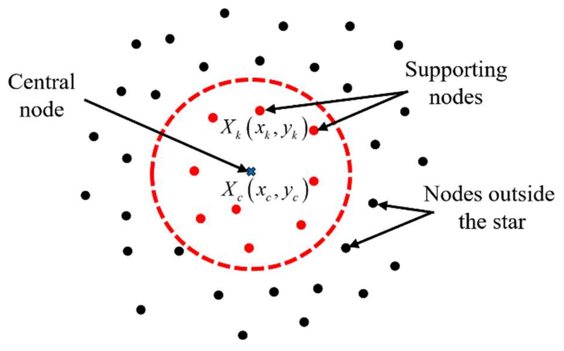
3. 2.5D GFDM for Elastic Wave Propagation Problems

Consider the model to be infinitely extended along the z-direction, with its mechanical and geometrical parameters invariant in this direction; that is, the material and geometry do not change along the z-axis. Therefore, it is convenient to solve the problem in the frequency-wavenumber domain, known as the 2.5D method. The problems described above are the type that the 2.5D method proposed in this paper aims to address. With z as the invariant direction, the governing equation and boundary conditions can be transformed to the frequency-wavenumber domain by applying the spatial Fourier transform to Equations (5)–(7) along the z-direction, as follows:

$${\alpha }^2\left(\tilde{\nabla }\tilde{\nabla }\cdot \tilde{\mathbf{u}}\right)-{\beta }^2\tilde{\nabla }\times \tilde{\nabla }\times \tilde{\mathbf{u}}+{\omega }^2\tilde{\mathbf{u}}=0,$$

(8)

$$\tilde{\mathbf{u}}={\tilde{\mathbf{u}}}_b,\tilde{\mathbf{x}}\in \tilde{\Gamma },$$

(9)

$$\tilde{\mathbf{t}}=\tilde{\mathit{\sigma }}\cdot \mathbf{n}={\tilde{\mathbf{t}}}_b\tilde{\mathbf{x}}\in \tilde{\Gamma },$$

(10)

where $\tilde{\nabla }=\left[{\displaystyle \frac{\partial }{\partial x}},{\displaystyle \frac{\partial }{\partial y}},\mathrm{i}{k}_z\right]$ is the Fourier transform of the gradient operator $\nabla =\left[{\displaystyle \frac{\partial }{\partial x}},{\displaystyle \frac{\partial }{\partial y}},{\displaystyle \frac{\partial }{\partial z}}\right]$,

$$\tilde{\mathbf{t}}\left(x,y,k_z\right)={\displaystyle {\int }_{-\infty }^{+\infty }\mathbf{t}\left(x,y,z\right)e^{-\mathrm{i}{k}_{z}z}dz},$$

(11)

$$\tilde{\mathbf{u}}\left(x,y,k_z\right)={\displaystyle {\int }_{-\infty }^{+\infty }\mathbf{u}\left(x,y,z\right)e^{-i{k}_{z}z}dz},$$

(12)

in which

$$\mathbf{u}\left(x,y,z\right)={\displaystyle \frac{1}{2\pi }}{\displaystyle {\int }_{-\infty }^{+\infty }\tilde{\mathbf{u}}\left(x,y,k_z\right)e^{\mathrm{i}{k}_{z}z}d{k}_z}.$$

(13)

It can be observed that the derivatives related to $z$ are replaced by $k_z$ which represents the spatial wavenumber associated with the longitudinal z-direction, $\mathrm{i}$ denotes the imaginary unit. The derivation detailed in [68] provides a comprehensive development of the described procedure; for the sake of conciseness, it is omitted from the present manuscript.

The integral resembling the inverse Fourier transform is computed using numerical methods. However, the approximate solution $\tilde{\mathbf{u}}$ exhibits singular behavior at $\left|k_z\right|=k_p$ or $\left|k_z\right|=k_s$. To circumvent the issue of singular values during the integration and to enhance the precision of the computation, a novel formulation for Equation (13) has been developed, which is as follows:

$$\mathbf{u}\left(x,y,z\right)={\mathbf{u}}_1\left(x,y,z\right)+{\mathbf{u}}_2\left(x,y,z\right)+{\mathbf{u}}_3\left(x,y,z\right)+{\mathbf{u}}_4\left(x,y,z\right)+{\mathbf{u}}_5\left(x,y,z\right),$$

(14)

in which

$$\begin{array}{l}{\mathbf{u}}_1\left(x,y,z\right)={\displaystyle \frac{1}{2\pi }}{\displaystyle {\int }_{-\infty }^{-{\beta }_2{k}_s}\tilde{\mathbf{u}}\left(x,y,k_z\right)e^{\mathrm{i}{k}_{z}z}d{k}_z}\\ +{\displaystyle \frac{1}{2\pi }}{\displaystyle {\int }_0^{-k_s\sqrt{{\beta }_2^2-1}}\tilde{\mathbf{u}}\left(x,y,w_{sl}\right)e^{\mathrm{i}\sqrt{k_s^2+w_{sl}^2}z}\frac{w_{sl}}{\sqrt{k_s^2-w_{sl}^2}}d{w}_{sl}},\end{array}$$

(15)

$$\begin{array}{l}{\mathbf{u}}_2\left(x,y,z\right)={\displaystyle \frac{1}{2\pi }}{\displaystyle {\int }_0^{-k_s\sqrt{1-{\beta }_1^2}}\tilde{\mathbf{u}}\left(x,y,v_{sl}\right)e^{\mathrm{i}\sqrt{k_s^2-v_{sl}^2}z}\frac{v_{sl}}{\sqrt{k_s^2-v_{sl}^2}}d{v}_{sl}}\\ +{\displaystyle \frac{1}{2\pi }}{\displaystyle {\int }_{-{\beta }_1{k}_s}^{-{\beta }_2{k}_p}\tilde{\mathbf{u}}\left(x,y,k_z\right)e^{\mathrm{i}{k}_{z}z}d{k}_z}\\ +{\displaystyle \frac{1}{2\pi }}{\displaystyle {\int }_0^{-k_p\sqrt{{\beta }_2^2-1}}\tilde{\mathbf{u}}\left(x,y,w_{pr}\right)e^{\mathrm{i}\sqrt{k_p^2+w_{pr}^2}z}\frac{w_{pr}}{\sqrt{k_p^2+w_{pr}^2}}d{w}_{pr}},\end{array}$$

(16)

$$\begin{array}{l}{\mathbf{u}}_3\left(x,y,z\right)={\displaystyle \frac{1}{2\pi }}{\displaystyle {\int }_0^{-k_p\sqrt{1-{\beta }_1^2}}\tilde{\mathbf{u}}\left(x,y,v_{pl}\right)e^{-\mathrm{i}\sqrt{k_p^2-v_{pl}^2}z}\frac{v_{pl}}{\sqrt{k_p^2-v_{pl}^2}}d{v}_{pl}}\\ +{\displaystyle \frac{1}{2\pi }}{\displaystyle {\int }_{-{\beta }_1{k}_p}^{{\beta }_1{k}_p}\tilde{\mathbf{u}}\left(x,y,k_z\right)e^{\mathrm{i}{k}_{z}z}d{k}_z}\\ +{\displaystyle \frac{1}{2\pi }}{\displaystyle {\int }_0^{k_p\sqrt{1-{\beta }_1^2}}\tilde{\mathbf{u}}\left(x,y,v_{pr}\right)e^{\mathrm{i}\sqrt{k_p^2-v_{pr}^2}z}\frac{v_{pr}}{\sqrt{k_p^2-v_{pr}^2}}d{v}_{pr}},\end{array}$$

(17)

$$\begin{array}{l}{\mathbf{u}}_4\left(x,y,z\right)={\displaystyle \frac{1}{2\pi }}{\displaystyle {\int }_0^{k_p\sqrt{{\beta }_2^2-1}}\tilde{\mathbf{u}}\left(x,y,w_{pl}\right)e^{\mathrm{i}\sqrt{k_p^2+w_{pl}^2}z}\frac{w_{pl}}{\sqrt{k_p^2+w_{pl}^2}}d{w}_{pl}}\\ +{\displaystyle \frac{1}{2\pi }}{\displaystyle {\int }_{{\beta }_2{k}_p}^{{\beta }_1{k}_s}\tilde{\mathbf{u}}\left(x,y,k_z\right)e^{\mathrm{i}{k}_{z}z}d{k}_z}\\ +{\displaystyle \frac{1}{2\pi }}{\displaystyle {\int }_{k_s}^{k_s\sqrt{1-{\beta }_1^2}}\tilde{\mathbf{u}}\left(x,y,v_{sr}\right)e^{\mathrm{i}\sqrt{k_s^2-v_{sr}^2}z}\frac{v_{sr}}{\sqrt{k_s^2-v_{sr}^2}}d{v}_{sr}},\end{array}$$

(18)

$$\begin{array}{l}{\mathbf{u}}_5\left(x,y,z\right)={\displaystyle \frac{1}{2\pi }}{\displaystyle {\int }_{k_s}^{k_s\sqrt{{\beta }_2^2-1}}\tilde{\mathbf{u}}\left(x,y,w_{sr}\right)e^{\mathrm{i}\sqrt{k_s^2+w_{sr}^2}z}\frac{w_{sr}}{\sqrt{k_s^2+w_{sr}^2}}d{w}_{sr}}\\ +{\displaystyle \frac{1}{2\pi }}{\displaystyle {\int }_{{\beta }_2{k}_s}^{+\infty }\tilde{\mathbf{u}}\left(x,y,k_z\right)e^{\mathrm{i}{k}_{z}z}d{k}_z},\end{array}$$

(19)

where $v_{pl}=-\sqrt{k_p^2-k_z^2},$ $v_{pr}=\sqrt{k_p^2-k_z^2},$ $v_{sl}=-\sqrt{k_s^2-k_z^2},$ $w_{pr}=-\sqrt{k_z^2-k_p^2},$ $w_{pl}=\sqrt{k_z^2-k_p^2},$ $v_{sr}=\sqrt{k_s^2-k_z^2},$ $w_{sl}=-\sqrt{k_z^2-k_s^2},$ $w_{sr}=\sqrt{k_z^2-k_s^2}$, $0<{\beta }_1<1$ and ${\beta }_2>1$. In this paper, the values of ${\beta }_1$ and ${\beta }_2$ are taken as 0.95 and 1.05. The integration limits are truncated at $\left|k_z\right|=k_p$ and $\left|k_z\right|=k_s$, being divided into five intervals. Each interval is further divided into singular integration limits, which are near singular points, and non-singular integration limits, which are away from singular points. For the integrals that fall within the singular limits, a variable substitution as shown in Equations (15)–(19) is applied, which enables the integration to bypass the singular points. It is noteworthy that during the calculation of the Fourier transform, the Hankel function experiences rapid decay when $\left|k_z\right|>k_s$. Consequently, to minimize computational resources, we have chosen the integration limits for Equation (14) to be $[-\gamma k_s,\gamma k_s]$.

For computational convenience, Equation (8) can be expressed in the following form:

$$\left\{\begin{array}{l}\left(\lambda +2\mu \right){\displaystyle \frac{{\partial }^2{\tilde{u}}_x}{\partial x^2}}+\mu {\displaystyle \frac{{\partial }^2{\tilde{u}}_x}{\partial y^2}}+\left({\omega }^2\rho -\mu k_z^2\right){\tilde{u}}_x+\left(\lambda +\mu \right){\displaystyle \frac{{\partial }^2{\tilde{u}}_y}{\partial x\partial y}}+\mathrm{i}{k}_z\left(\lambda +\mu \right){\displaystyle \frac{\partial {\tilde{u}}_z}{\partial x}}=0\\ \left(\lambda +2\mu \right){\displaystyle \frac{{\partial }^2{\tilde{u}}_y}{\partial y^2}}+\mu {\displaystyle \frac{{\partial }^2{\tilde{u}}_y}{\partial x^2}}+\left({\omega }^2\rho -\mu k_z^2\right){\tilde{u}}_y+\left(\lambda +\mu \right){\displaystyle \frac{{\partial }^2{\tilde{u}}_x}{\partial x\partial y}}+\mathrm{i}{k}_z\left(\lambda +\mu \right){\displaystyle \frac{\partial {\tilde{u}}_z}{\partial y}}=0\\ \mathrm{i}{k}_z\left(\lambda +\mu \right){\displaystyle \frac{\partial {\tilde{u}}_x}{\partial x}}+\mathrm{i}{k}_z\left(\lambda +\mu \right){\displaystyle \frac{\partial {\tilde{u}}_y}{\partial y}}+\mu {\displaystyle \frac{{\partial }^2{\tilde{u}}_z}{\partial x^2}}+\mu {\displaystyle \frac{{\partial }^2{\tilde{u}}_z}{\partial y^2}}+\left[{\omega }^2\rho -k_z^2\left(\lambda +2\mu \right)\right]{\tilde{u}}_z=0\end{array}\right..$$

(20)

The above equation can be defined as a 2D equation of $\left[{\tilde{u}}_x,{\tilde{u}}_y,{\tilde{u}}_z\right]=\tilde{\mathbf{u}}\left(x,y,k_z\right)$. By applying Equation (13), we can compute the 3D displacement field $\mathbf{u}\left(x,y,z\right)$ in the frequency domain by solving $\tilde{\mathbf{u}}\left(x,y,k_z\right)$ for every $k_z$.

The problem (5) will be solved by the 2.5D generalized finite difference method (2.5D GFDM), a meshless method developed from Taylor series expansion of multivariate functions and weighted moving least squares. The 2.5D approach enables the solution of 3D problems by utilizing a wavenumber-dependent 2D cross-sectional formulation. In this study, the z-direction is designated as the axis of geometrical invariance, allowing the reduction of the discretization domain from three dimensions to two. Within the 2.5D framework, the location of any given point is specified by a pair of values in a vector, which correspond to its Cartesian coordinates within the cross-sectional plane of the system. In contrast, displacements and tractions are represented by three-element vectors that capture their values along each of the three coordinate axes. Therefore, the mathematical procedures of the GFDM will be illustrated using the 2D case as an example.

In the GFDM, the derivative of an uncharted variable in the governing equation is estimated through a linear combination of the function values at its adjacent nodes. For numerical simulation, a set of $N_b$ boundary nodes and $N_i$ interior nodes are distributed uniformly or randomly along the boundary $\Gamma$ and in the computational domain $\Omega$, respectively. For a designated $i^{th}$ node $X_c\left(x_c,y_c\right)$ named the central node, the m surrounding nodes $X_k\left(x_k,y_k\right)\left(k=1,2,\dots ,m\right)$ within proximity, along with the central node, are enclosed within a circular perimeter to create a supporting domain star, as depicted in Figure 1. A review of prior research [45,49] suggests that the stability and precision of numerical solutions are ensured when the $m$ is greater than 10.

With the central node $X_c$ designated and its corresponding star established, the Taylor series expansion for each node within the star can be utilized to expand the function, as described subsequently:

$$u_k=u_c+h_k{\displaystyle \frac{\partial u_c}{\partial x}}+l_k{\displaystyle \frac{\partial u_c}{\partial y}}+{\displaystyle \frac{h_k^2}{2}}{\displaystyle \frac{{\partial }^2{u}_c}{\partial x^2}}+{\displaystyle \frac{l_k^2}{2}}{\displaystyle \frac{{\partial }^2{u}_c}{\partial y^2}}+h_k{l}_k{\displaystyle \frac{{\partial }^2{u}_c}{\partial x\partial y}}+\cdots ,k=1,2,\dots ,m.$$

(21)

where $h_k$ and $l_k$ denote the distance between the supporting node $X_k\left(x_k,y_k\right)\left(k=1,2,\dots ,m\right)$ and the central node $X_c\left(x_c,y_c\right)$ in x- and y-directions:

$$h_k=x_k-x_c,k=1,2,\dots ,m.$$

(22)

$$l_k=y_k-y_c,k=1,2,\dots ,m.$$

(23)

$u_k=u\left(x_k,y_k\right)$ and $u_c=u\left(x_c,y_c\right)$ denote the function value at the nodes $X_k\left(x_k,y_k\right)\left(k=1,2,\dots ,m\right)$ and $X_c\left(x_c,y_c\right)$, respectively. ${\displaystyle \frac{\partial u_c}{\partial x}},$ ${\displaystyle \frac{\partial u_c}{\partial y}},$ ${\displaystyle \frac{{\partial }^2{u}_c}{\partial x^2}},$ ${\displaystyle \frac{{\partial }^2{u}_c}{\partial y^2}},$ ${\displaystyle \frac{{\partial }^2{u}_c}{\partial x\partial y}},$ are the derivatives at the node $X_c\left(x_c,y_c\right)$. By limiting the Taylor series expansions to include only up to the second-order derivatives, the residual function $B(u)$ is defined in the subsequent manner:

$$B(u)={{\displaystyle \sum _{k=1}^m\left[\left(u_c-u_k+h_k\frac{\partial u_c}{\partial x}+l_k\frac{\partial u_c}{\partial x}+\frac{h_k^2}{2}\frac{{\partial }^2{u}_c}{\partial x^2}+\frac{l_k^2}{2}\frac{{\partial }^2{u}_c}{\partial y^2}+h_k{l}_k\frac{{\partial }^2{u}_c}{\partial x\partial y}\right)w_k\right]}}^2,$$

(24)

in which $w_k$ is the weighting coefficient at $X_k$ and represents the importance of the approximations by Taylor series expansion at different nodes in the star of the node $X_c$. The weighting coefficient suggests that the Taylor series approximation at a node $X_k$ is more influential if the node is in closer proximity to the central node $X_c$. With greater separation from a node $X_c$, the weight coefficient exhibits a corresponding reduction. A multitude of options for the weighting coefficient can be found in the extant literature [69], including potential functions and cubic splines, among others. In this study, the weighting coefficient is adopted in the following form:

$$w_k=\left\{\begin{array}{cc}1-6{\left({\displaystyle \frac{d_k}{d_m}}\right)}^2+8{\left({\displaystyle \frac{d_k}{d_m}}\right)}^3-3{\left({\displaystyle \frac{d_k}{d_m}}\right)}^4,& d_k\le d_m,\\ 0,& d_k>d_m,\end{array}\right.$$

(25)

in which $d_k=\sqrt{h_k^2+l_k^2}$ denotes the distance between nodes $X_k$ and $X_c$, and $d_m$ represents the distance between the farthest node and the node $X_c$ within the star. The partial derivatives at a node $X_c$ appeared in Equation (24) are represented by

$${\mathit{D}}_u={\left[{\left.{\displaystyle \frac{\partial u_c}{\partial x}}\right|}_{X_c},{\left.{\displaystyle \frac{\partial u_c}{\partial y}}\right|}_{X_c},{\left.{\displaystyle \frac{{\partial }^2{u}_c}{\partial x^2}}\right|}_{X_c},{\left.{\displaystyle \frac{{\partial }^2{u}_c}{\partial y^2}}\right|}_{X_c},{\left.{\displaystyle \frac{{\partial }^2{u}_c}{\partial x\partial y}}\right|}_{X_c}\right]}^{\mathbf{T}}.$$

(26)

In practical applications, it is preferable for the above residual function $B(u)$ to be minimized with respect to the partial derivatives ${\mathit{D}}_u$, i.e.,

$${\displaystyle \frac{\partial B(u)}{\partial \left\{{\mathit{D}}_u\right\}}}=0,$$

(27)

and the linear system of equations will be yielded as follows:

$$\mathit{A}{\mathit{D}}_{\mathit{u}}=\mathit{b},$$

(28)

in which

$$\mathit{A}=\left[\begin{array}{ccccc}{\displaystyle \sum _{k=1}^m{w}_k^2{h}_k^2}& {\displaystyle \sum _{k=1}^m{w}_k^2{h}_k{l}_k}& {\displaystyle \sum _{k=1}^m{w}_k^2\frac{h_k^3}{2}}& {\displaystyle \sum _{k=1}^m{w}_k^2\frac{h_k{l}_k^2}{2}}& {\displaystyle \sum _{k=1}^m{w}_k^2{h}_k^2{l}_k}\\ & {\displaystyle \sum _{k=1}^m{w}_k^2{l}_k^2}& {\displaystyle \sum _{k=1}^m{w}_k^2\frac{h_k^2{l}_k}{2}}& {\displaystyle \sum _{k=1}^m{w}_k^2\frac{l_k^3}{2}}& {\displaystyle \sum _{k=1}^m{w}_k^2{h}_k{l}_k^2}\\ & & {\displaystyle \sum _{k=1}^m{w}_k^2\frac{h_k^4}{4}}& {\displaystyle \sum _{k=1}^m{w}_k^2\frac{h_k^2{l}_k^2}{4}}& {\displaystyle \sum _{k=1}^m{w}_k^2\frac{h_k^3{l}_k}{2}}\\ & SYM& & {\displaystyle \sum _{k=1}^m{w}_k^2\frac{l_k^4}{4}}& {\displaystyle \sum _{k=1}^m{w}_k^2\frac{h_k{l}_k^3}{2}}\\ & & & & {\displaystyle \sum _{k=1}^m{w}_k^2{h}_k^2{l}_k^2}\end{array}\right],$$

(29)

is the symmetric coefficient matrix, and the elements of matrix $\mathit{A}$ are obtained based on the spatial coordinates of the node $X_c$ and its neighboring nodes $X_k$. In addition,

$$\mathit{b}=\left[\begin{array}{l}{\displaystyle \sum _{k=1}^m{u}_k{w}_k^2{h}_k-u_c{\displaystyle \sum _{k=1}^m{w}_k^2{h}_k}}\\ {\displaystyle \sum _{k=1}^m{u}_k{w}_k^2{l}_k-u_c{\displaystyle \sum _{k=1}^m{w}_k^2{l}_k}}\\ {\displaystyle \sum _{k=1}^m{u}_k{w}_k^2\frac{h_k^2}{2}-u_c{\displaystyle \sum _{k=1}^m{w}_k^2\frac{h_k^2}{2}}}\\ {\displaystyle \sum _{k=1}^m{u}_k{w}_k^2\frac{l_k^2}{2}-u_c{\displaystyle \sum _{k=1}^m{w}_k^2\frac{l_k^2}{2}}}\\ {\displaystyle \sum _{k=1}^m{u}_k{w}_k^2{h}_k{l}_k-u_c{\displaystyle \sum _{k=1}^m{w}_k^2{h}_k{l}_k}}\end{array}\right],$$

(30)

which depends on the numerical variables and spatial coordinates of nodes inside the star, moreover, can be decomposed as

$$\mathit{b}=\mathit{B}\mathit{U},$$

(31)

in which

$$\mathit{B}={\left(-{\displaystyle \sum _{k=1}^m{w}_k{\mathit{A}}_2^{(k)},w_1{\mathit{A}}_2^{(1)},w_2{\mathit{A}}_2^{(2)},\dots ,w_m{\mathit{A}}_2^{(m)}}\right)}_{5\times (m+1)},$$

(32)

$$\mathit{U}={\left[u_c,u_1,u_2,\dots ,u_m\right]}^{\mathbf{T}},$$

(33)

where

$${\mathit{A}}_2^{(k)}={\displaystyle \frac{w_k}{2}}{\left[2h_k,2l_k,h_k^2,l_k^2,2h_k{l}_k\right]}^{\mathbf{T}}.$$

(34)

$u_i(i=c,1,2,3,\dots ,m)$ represents the vector of function values at the node $X_c$ and the other nodes $X_k$ within the star. ${\mathit{D}}_u$ can be described in an alternative form by merging Equation (28) with Equation (31) as follows:

$${\mathit{D}}_u={\mathit{A}}^{-1}\mathit{b}={\mathit{A}}^{-1}\left(\mathit{B}\mathit{U}\right)={\mathit{E}}^c\mathit{U},$$

(35)

where

$${\mathit{E}}^c={\mathit{A}}^{-1}\mathit{B}.$$

(36)

Drawing from the mathematical analysis provided, it is evident that for each central node $X_c$ within the computational domain, the derivatives of the unknown function at point $X_c$ can be approximated using a linear combination of the function values at the supporting nodes. Consequently, the partial derivatives at a central node can be articulated as follows:

$${\mathit{D}}_u=\left[\begin{array}{l}{\left.{\displaystyle \frac{\partial u_c}{\partial x}}\right|}_{X_c}\\ {\left.{\displaystyle \frac{\partial u_c}{\partial y}}\right|}_{X_c}\\ {\left.{\displaystyle \frac{{\partial }^2{u}_c}{\partial x^2}}\right|}_{X_c}\\ {\left.{\displaystyle \frac{{\partial }^2{u}_c}{\partial y^2}}\right|}_{X_c}\\ {\left.{\displaystyle \frac{{\partial }^2{u}_c}{\partial x\partial y}}\right|}_{X_c}\end{array}\right]=\left[\begin{array}{ccccc}{e}_{1c}^c& e_{11}^c& e_{12}^c& \dots & e_{1m}^c\\ e_{2c}^c& e_{21}^c& e_{22}^c& \dots & e_{2m}^c\\ e_{3c}^c& e_{31}^c& e_{32}^c& \dots & e_{3m}^c\\ e_{4c}^c& e_{41}^c& e_{42}^c& \dots & e_{4m}^c\\ e_{5c}^c& e_{51}^c& e_{52}^c& \dots & e_{5m}^c\end{array}\right]\left[\begin{array}{c}{u}_c\\ u_1\\ u_2\\ ⋮\\ u_m\end{array}\right],$$

(37)

in which each element $e_{ji}^c\left(j=1,2,\dots ,5;i=c,1,2,\dots ,m\right)$ of the matrix ${\mathit{E}}^c$ can be derived by Equation (36). It is imperative to apply the above procedures at every node within the computational domain and along the boundary to develop equations that substitute for the spatial derivatives at each node. By ensuring compliance with boundary conditions at the boundary nodes and adherence to the governing equations at the interior nodes, a system of linear algebraic equations is derived as

$$\left[\begin{array}{ccc}{\mathit{E}}_{1x}& {\mathit{E}}_{1y}& {\mathit{E}}_{1z}\\ {\mathit{E}}_{2x}& {\mathit{E}}_{2y}& {\mathit{E}}_{2z}\\ {\mathit{E}}_{3x}& {\mathit{E}}_{3y}& {\mathit{E}}_{3z}\end{array}\right]\left[\begin{array}{c}{\mathit{U}}_x^{all}\\ {\mathit{U}}_y^{all}\\ {\mathit{U}}_z^{all}\end{array}\right]=\left[\begin{array}{c}{\mathit{F}}_1\\ {\mathit{F}}_2\\ {\mathit{F}}_3\end{array}\right],$$

(38)

and can be written in matrix form:

$$\mathit{E}{\mathit{U}}^{all}=\mathit{F}.$$

(39)

Each matrix block in Equation (38) can be obtained from the above mathematical procedures. The numerical determination of function values at each node within the domain is accomplished by solving ${\mathit{U}}^{all}$ in Equation (39).

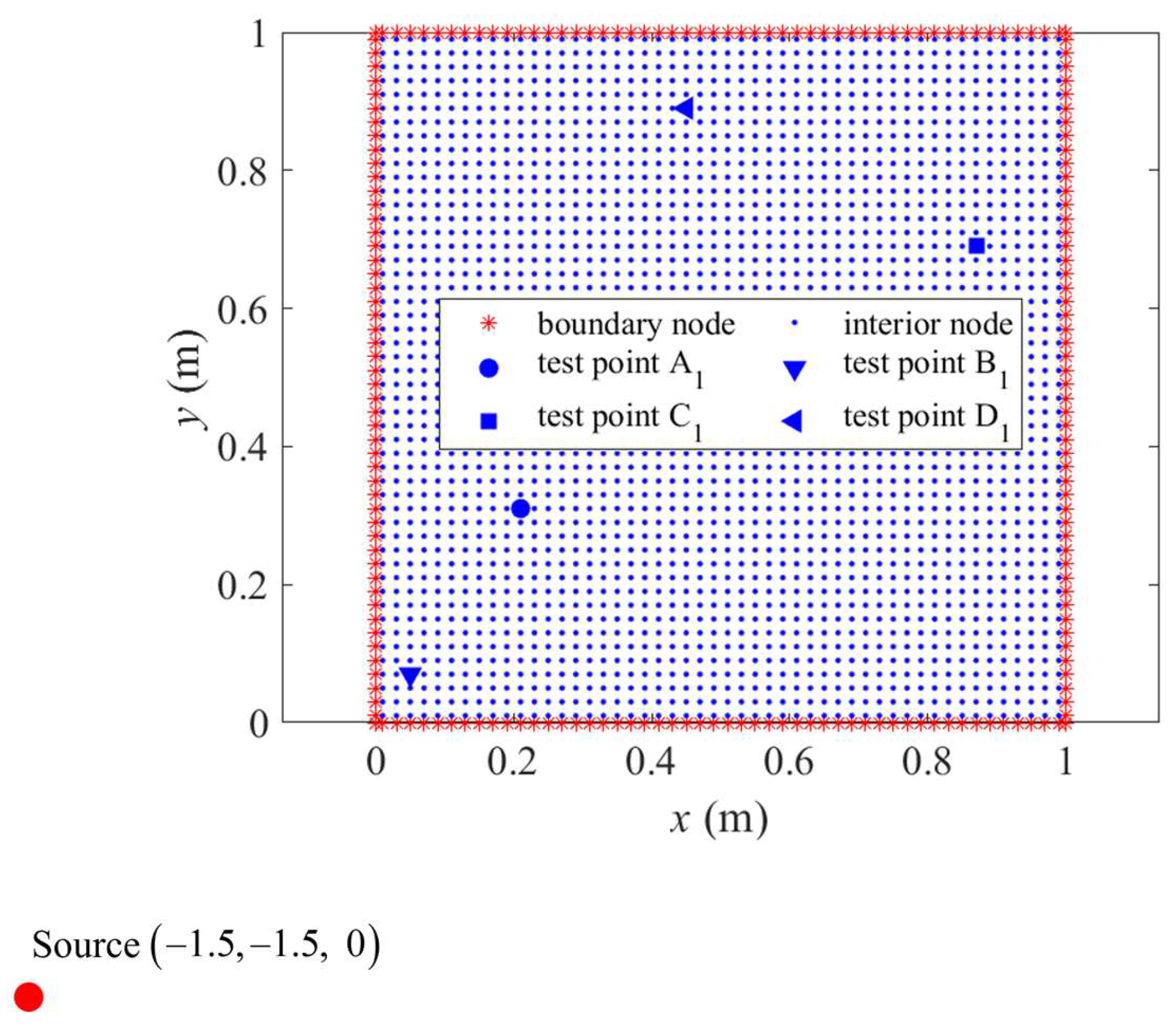
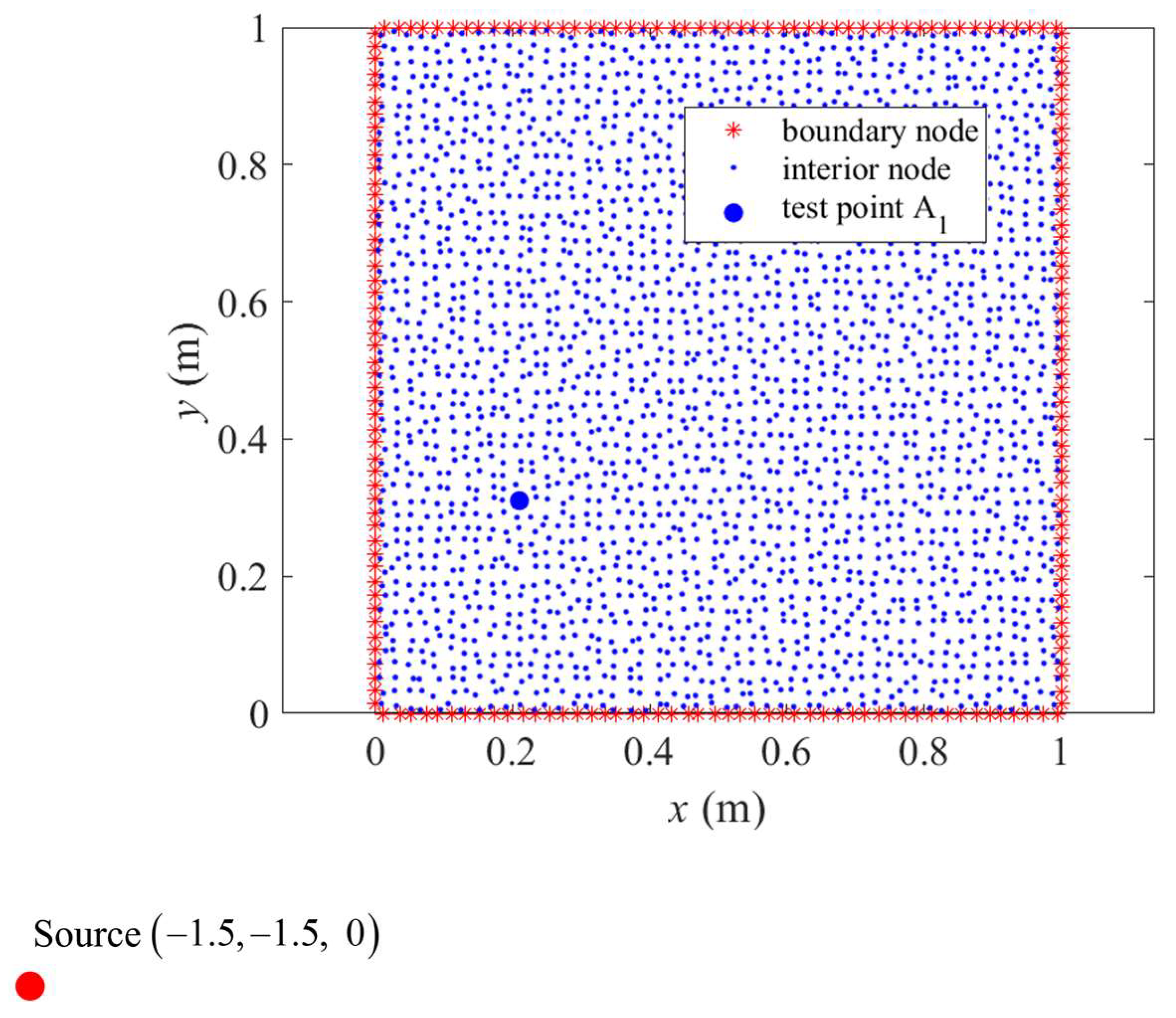
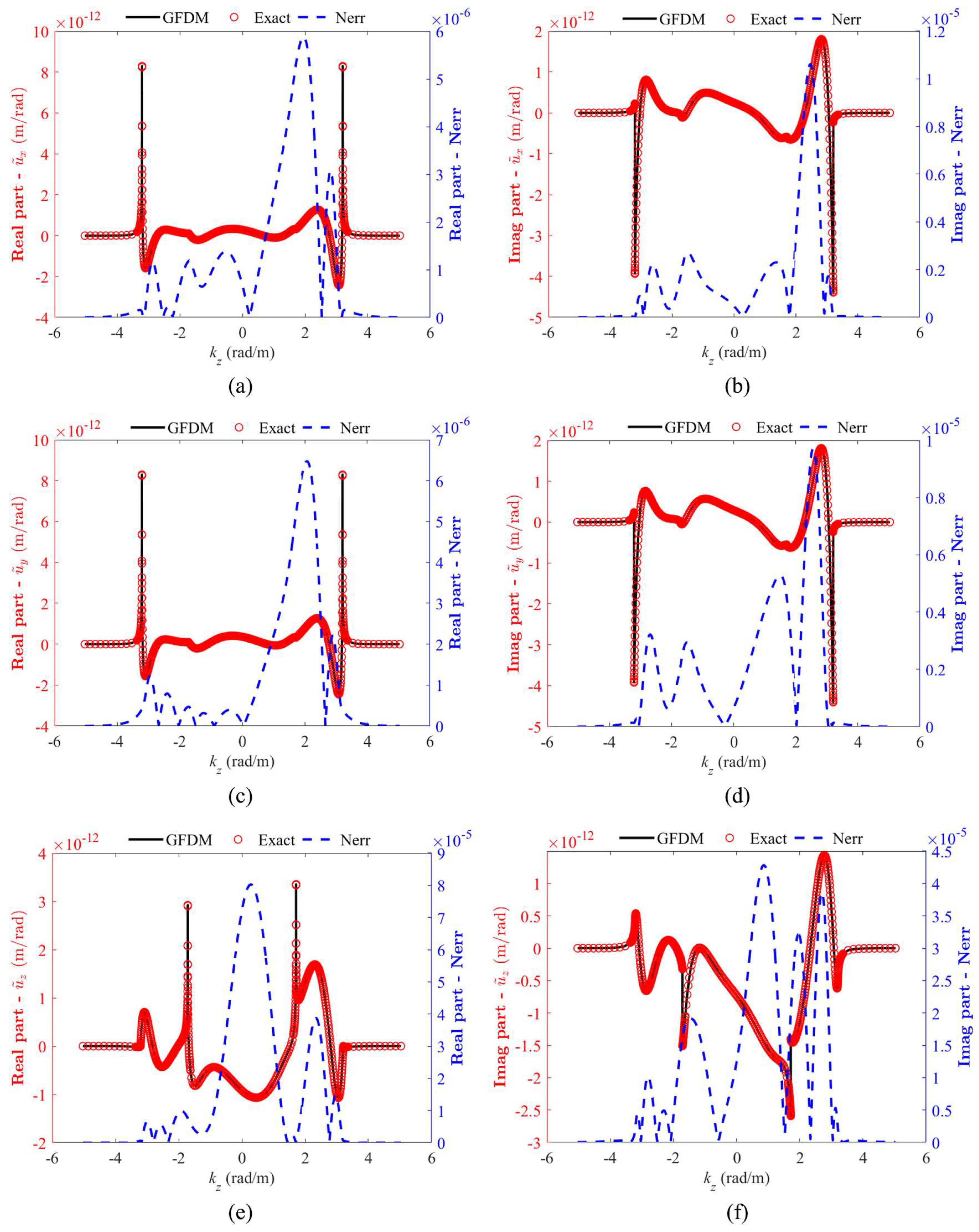
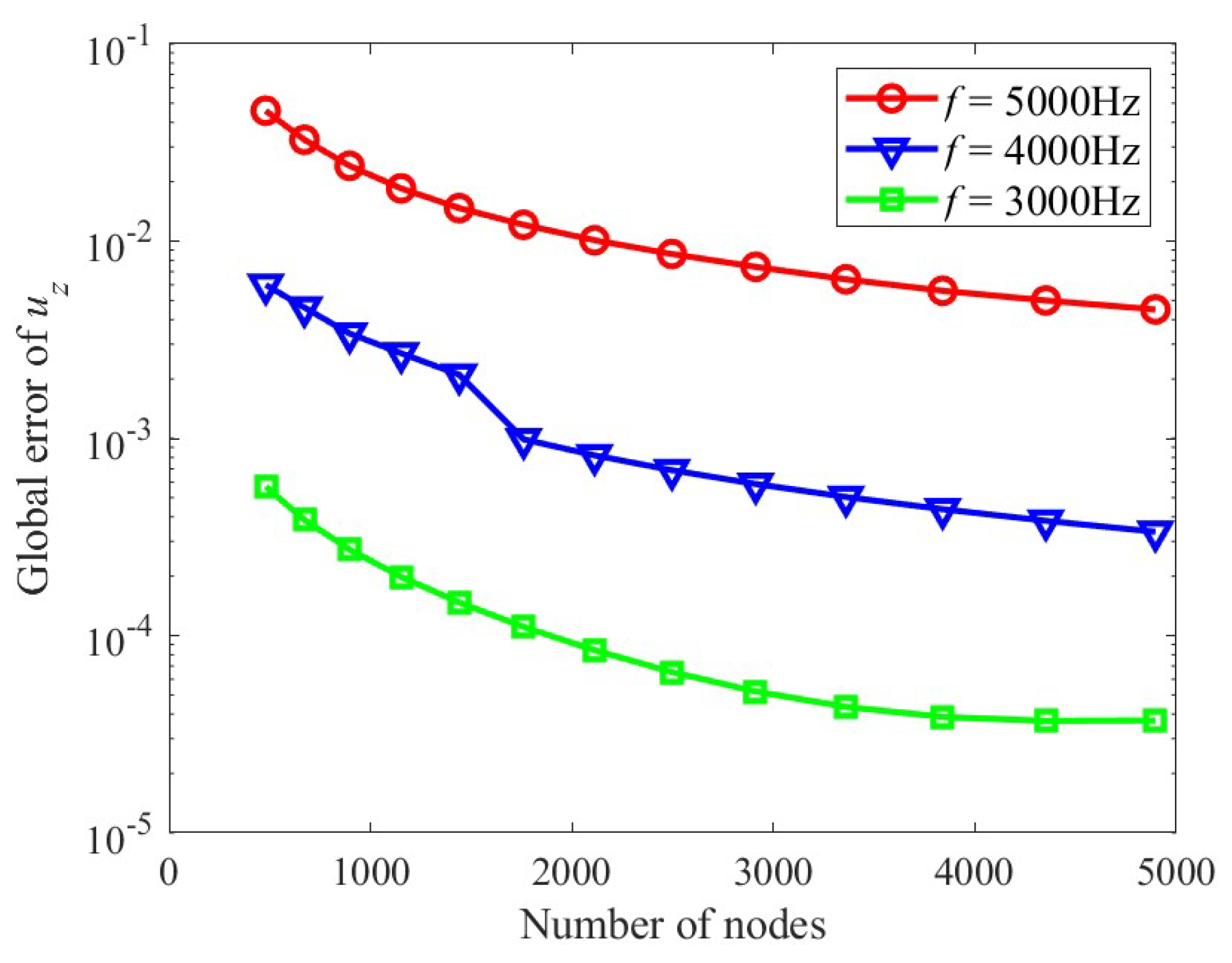
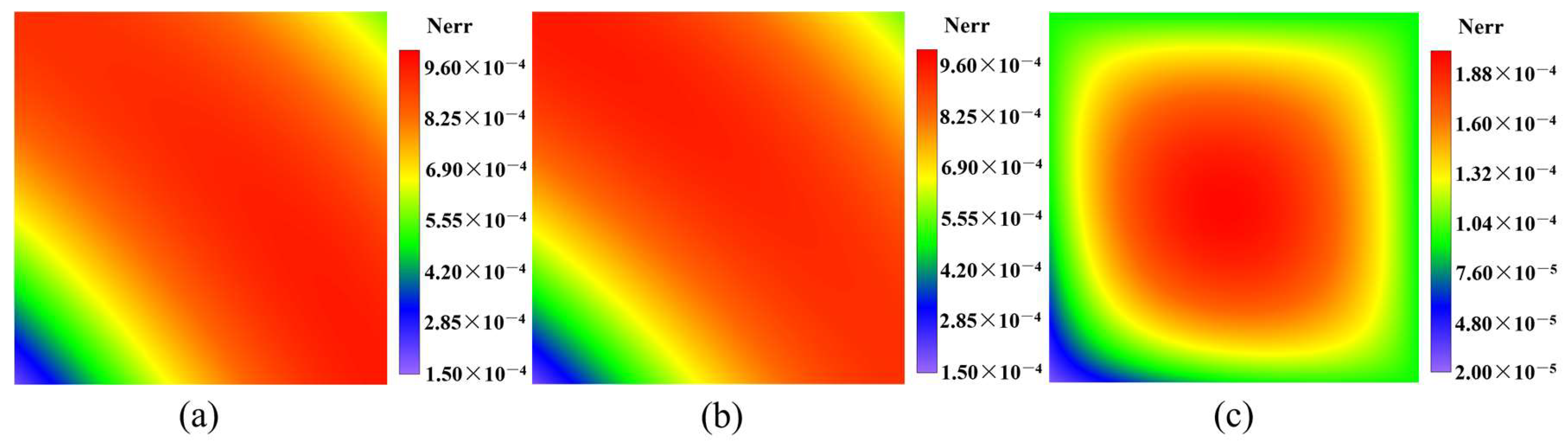
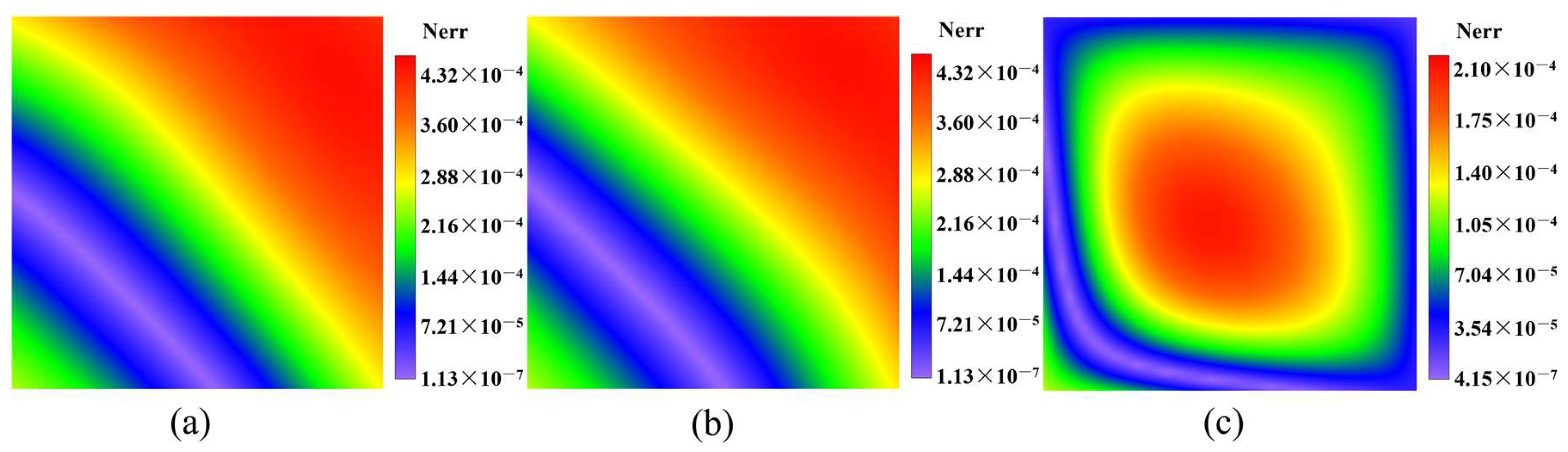
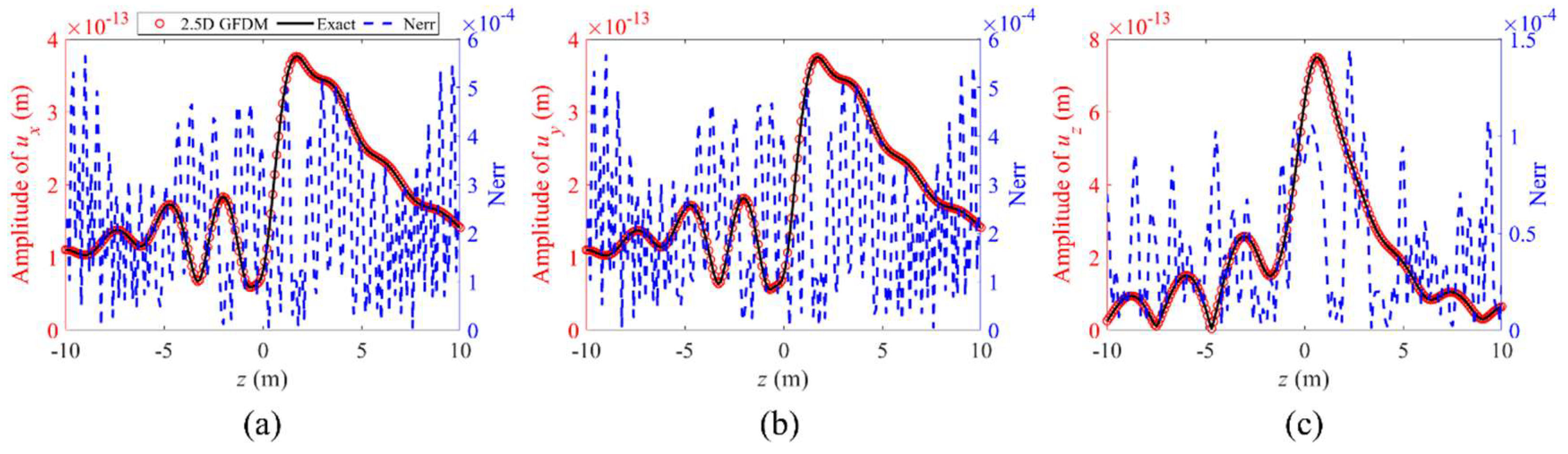
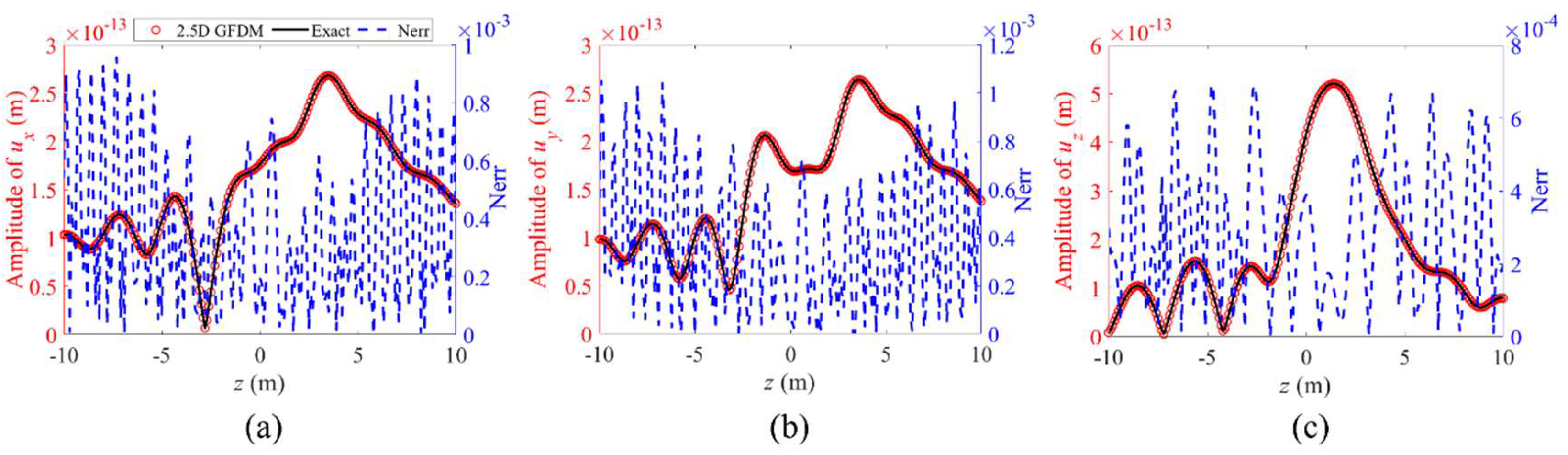
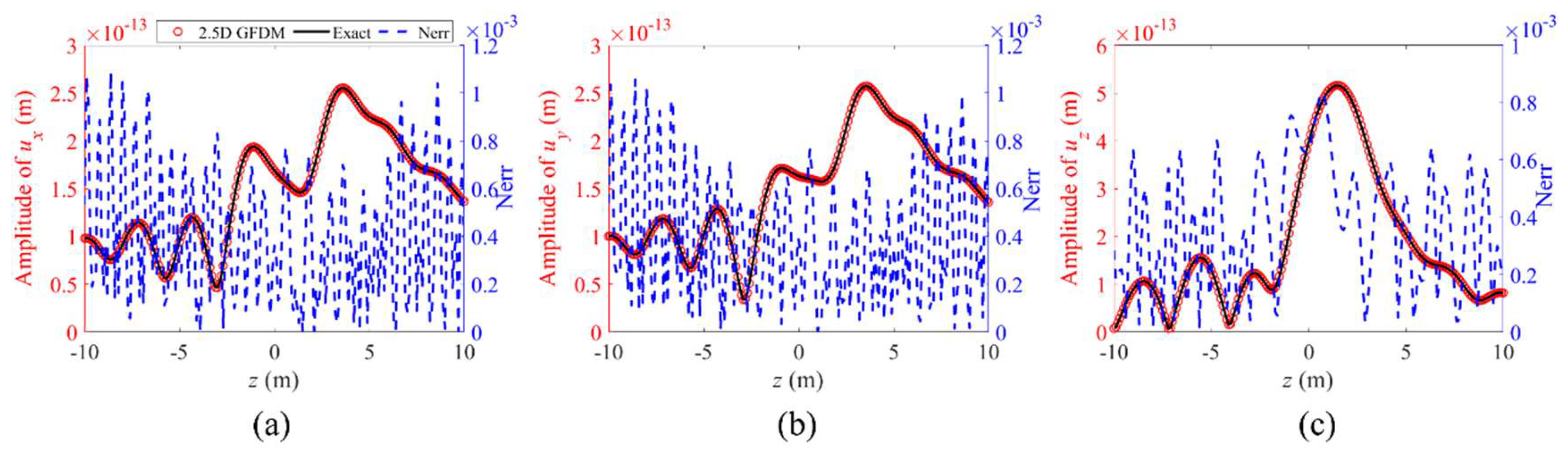
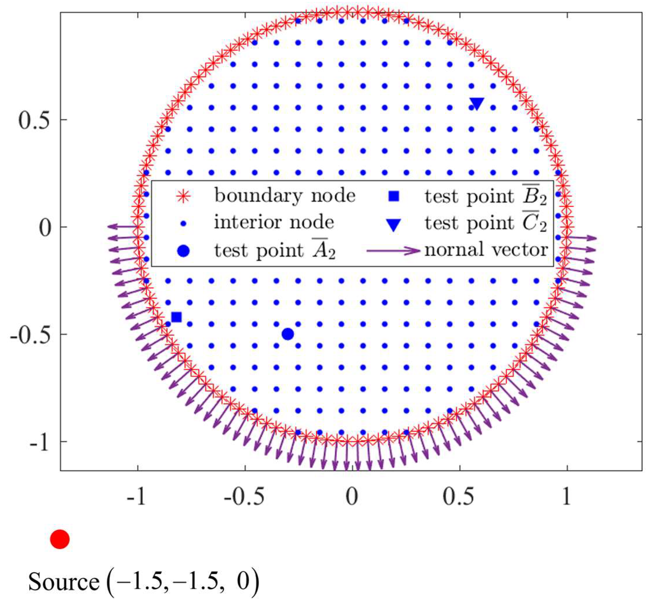
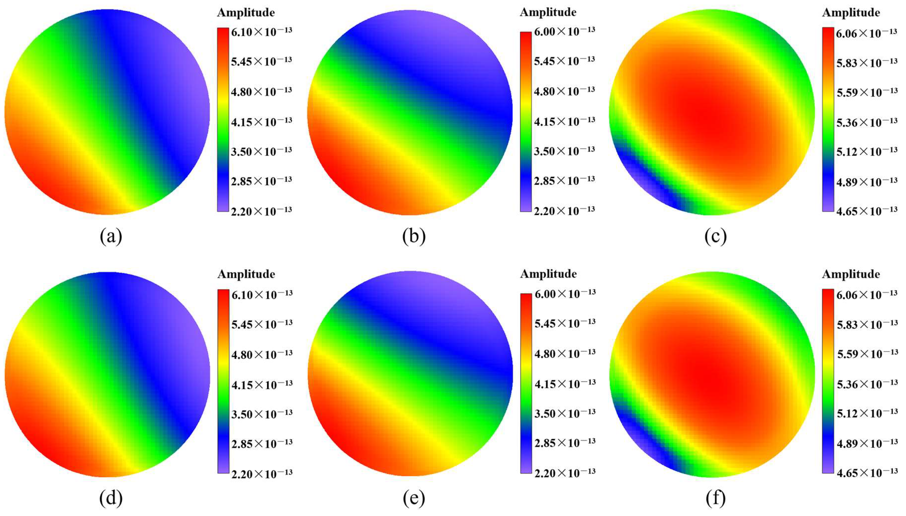
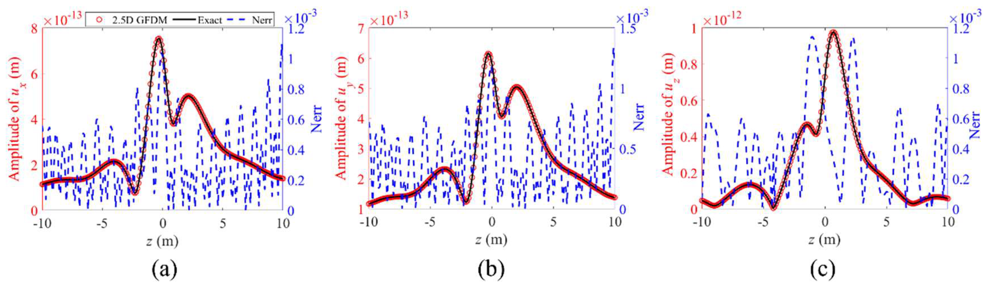
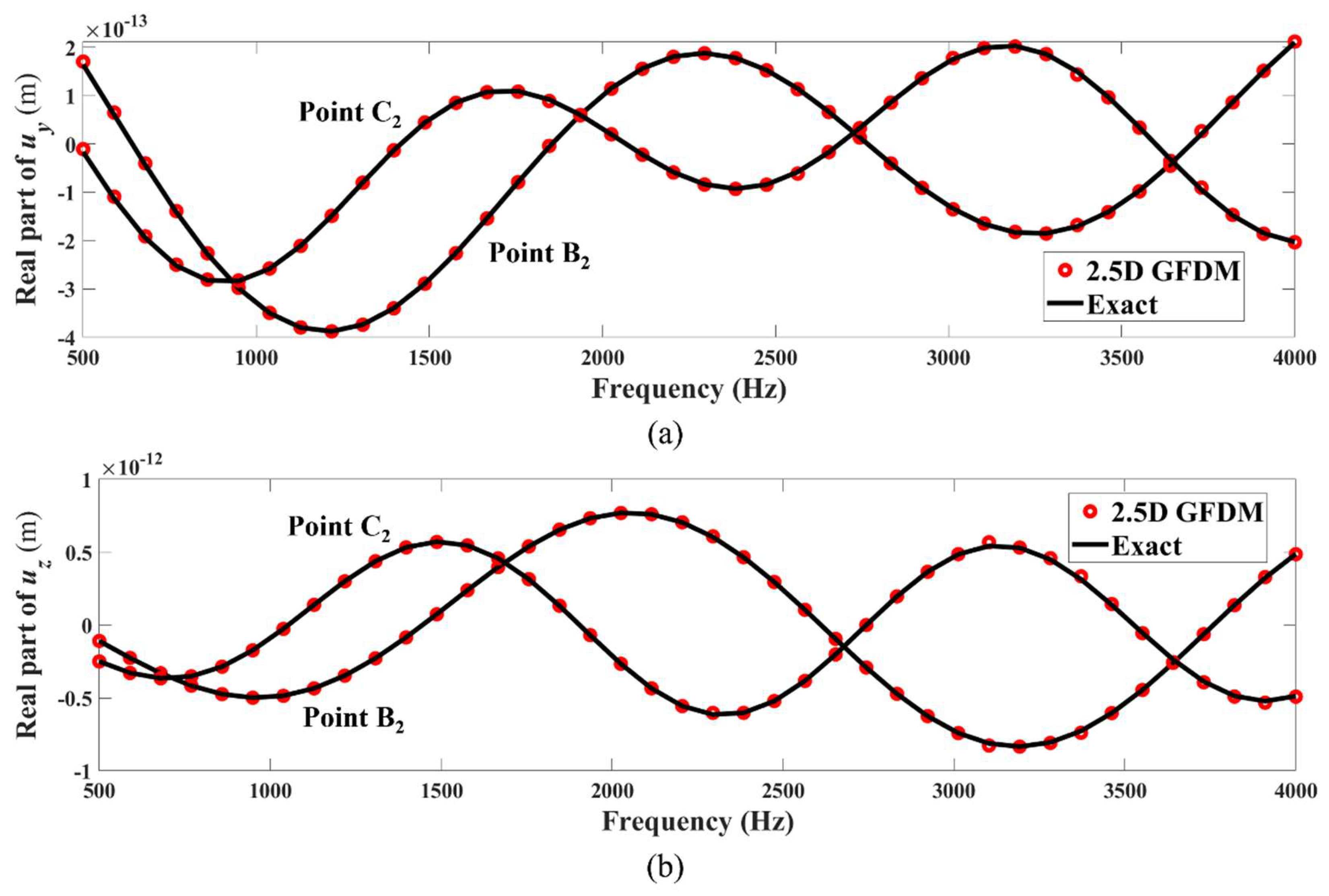
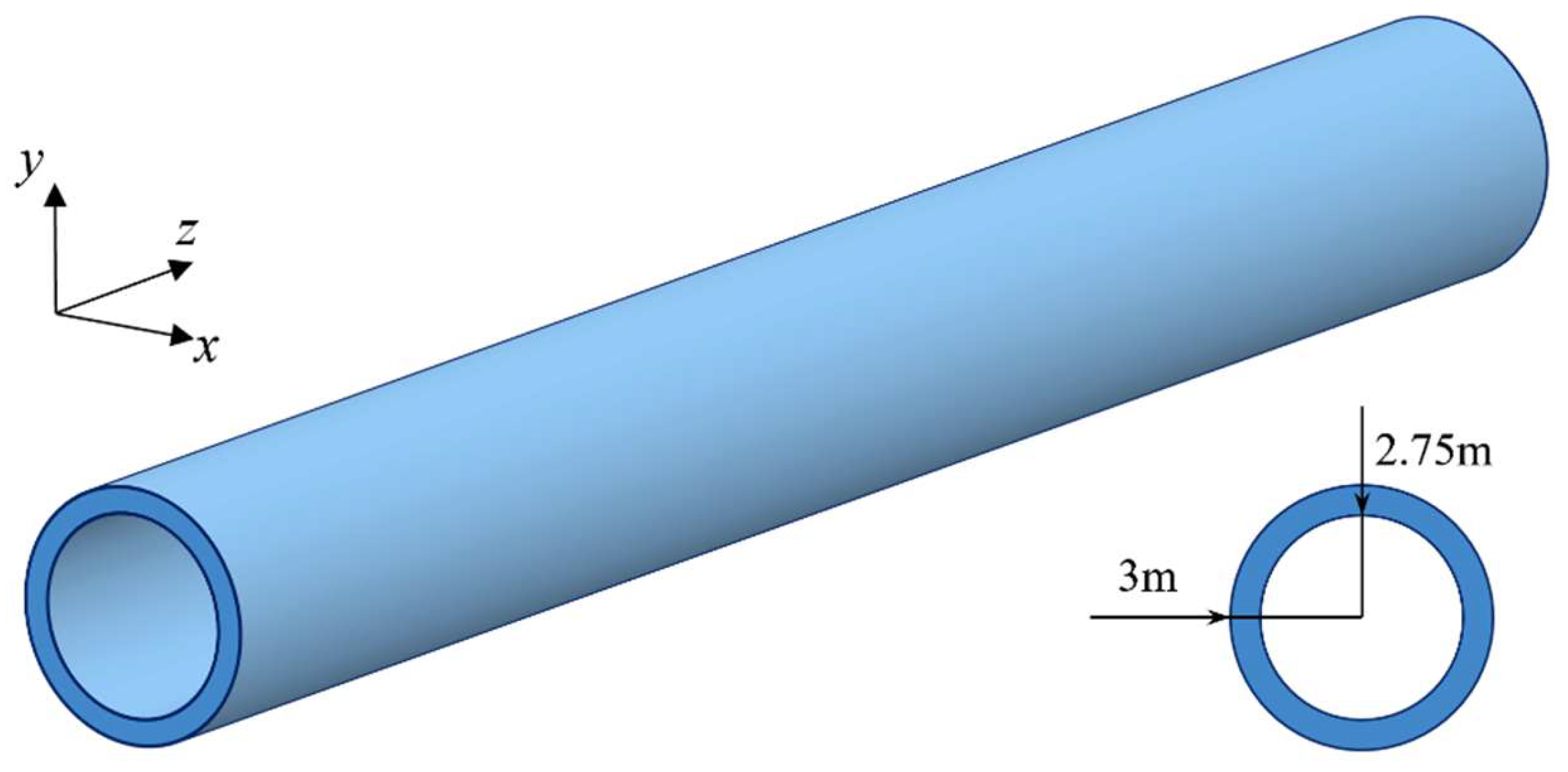
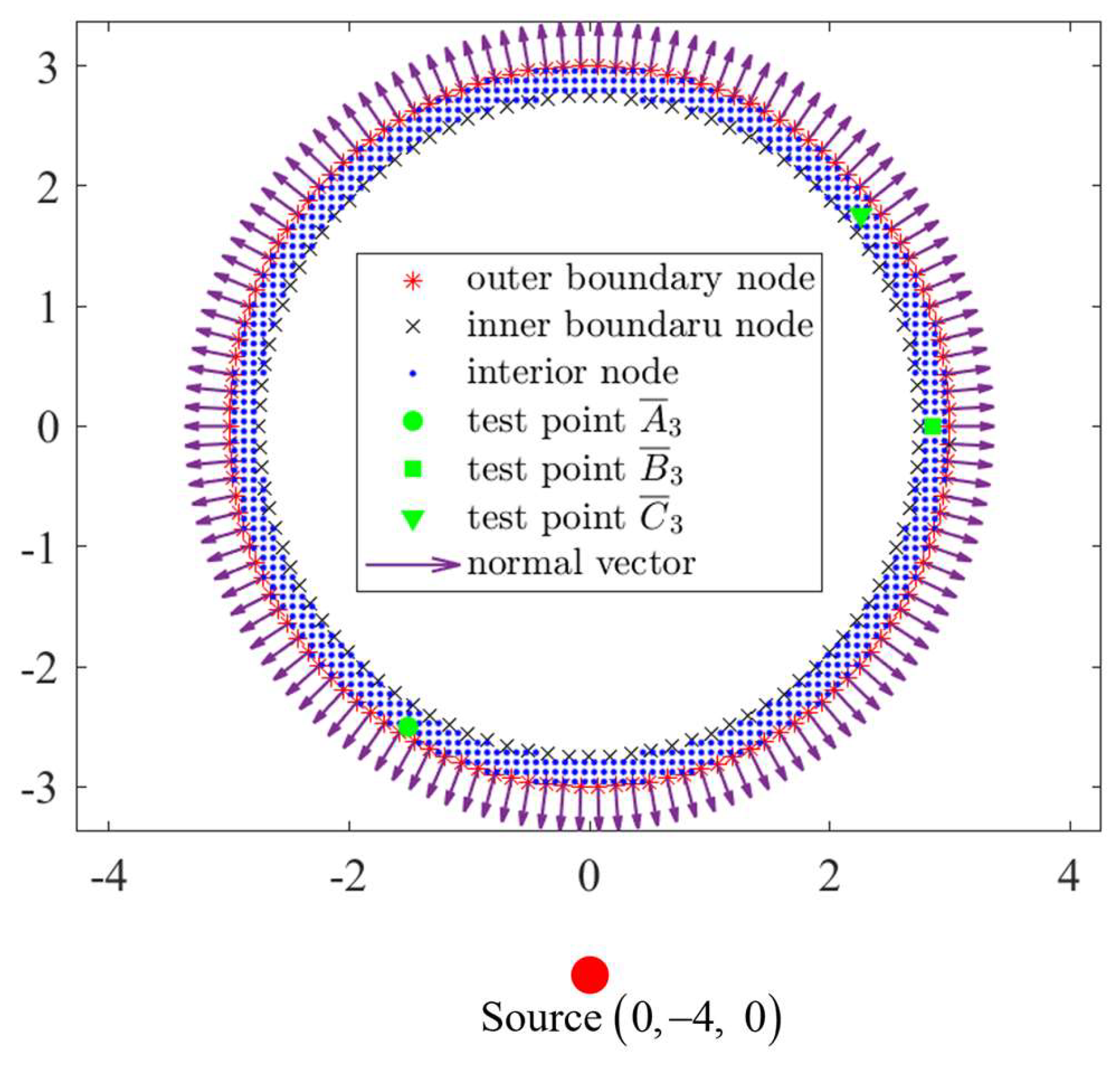
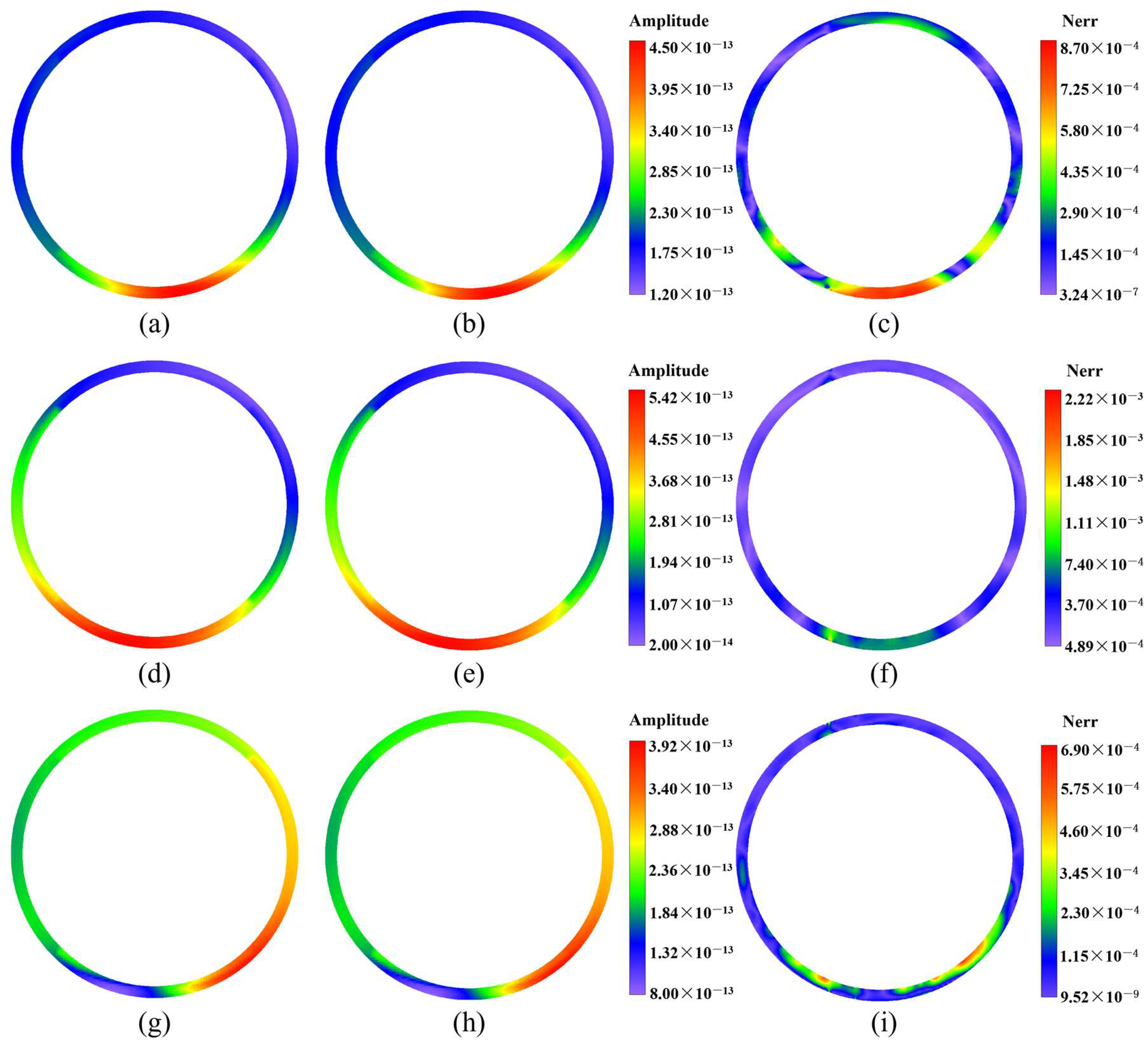
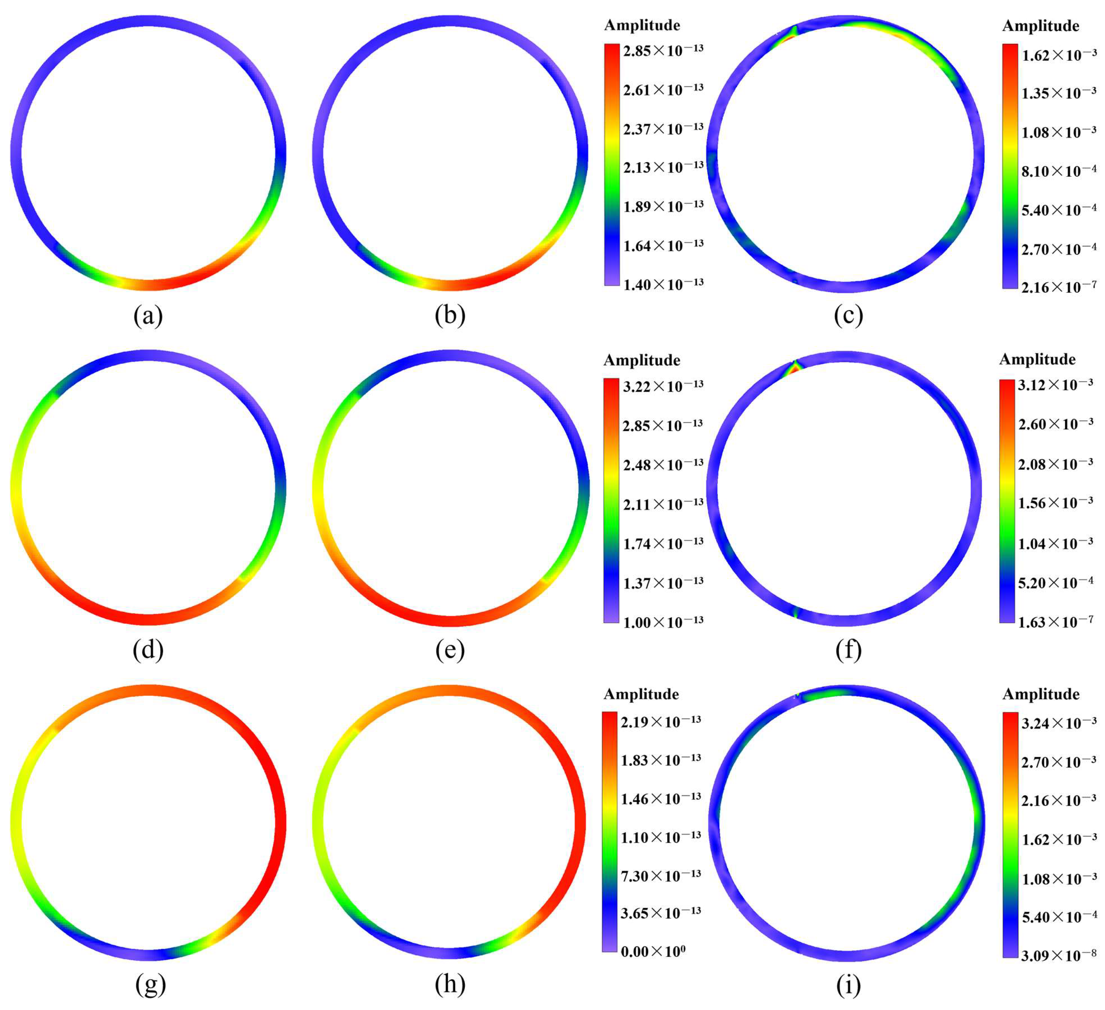
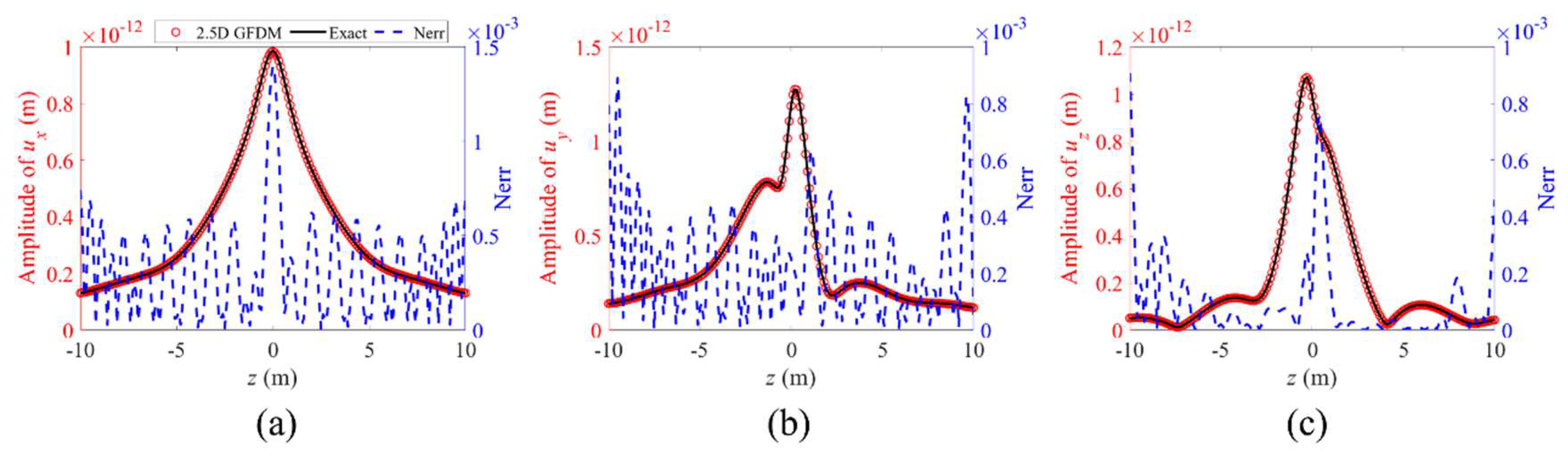
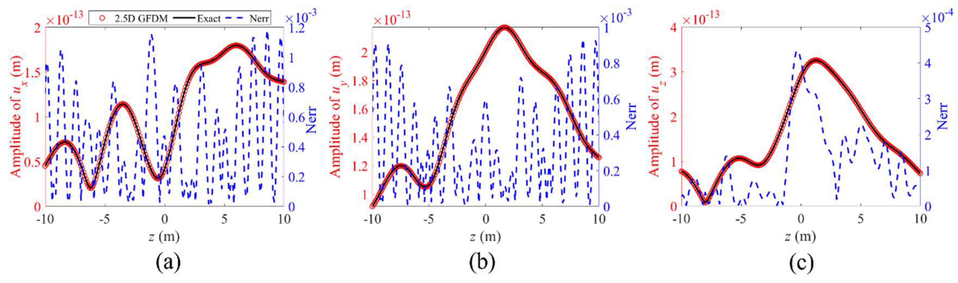
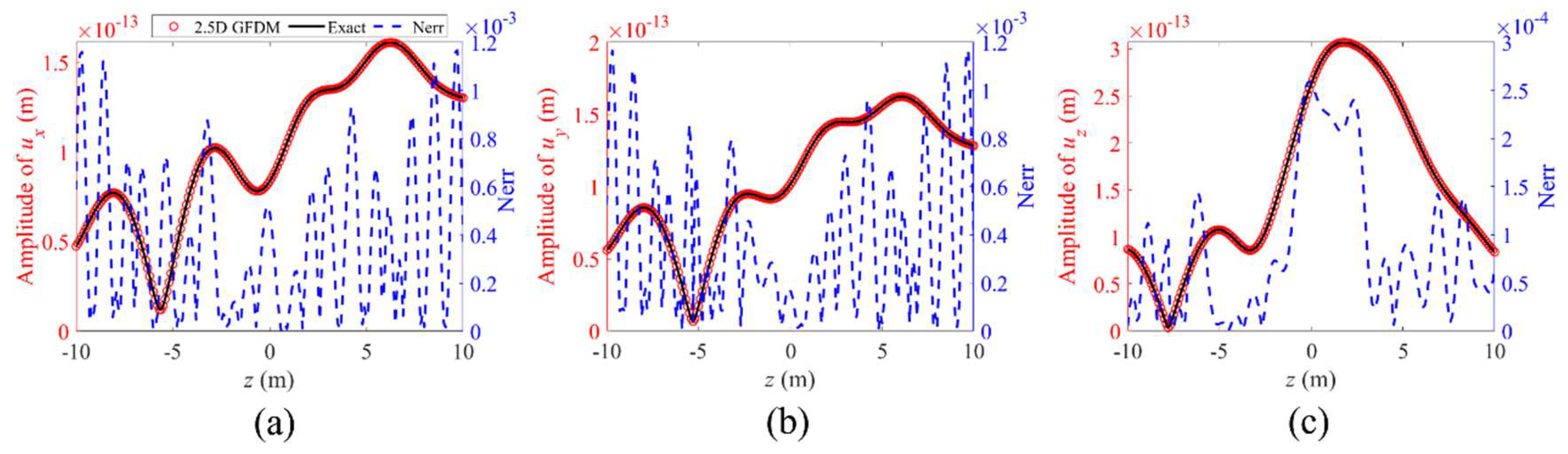
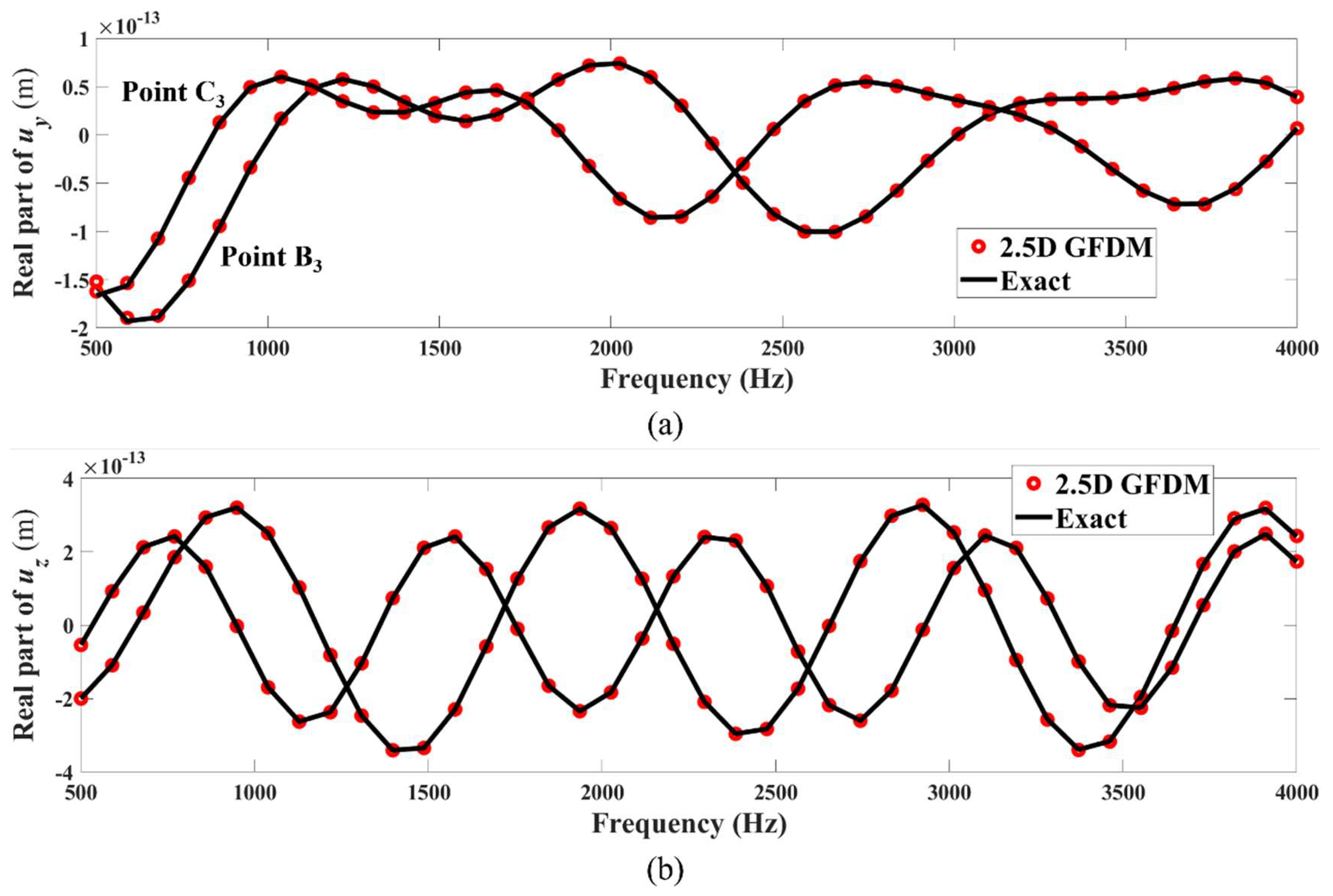
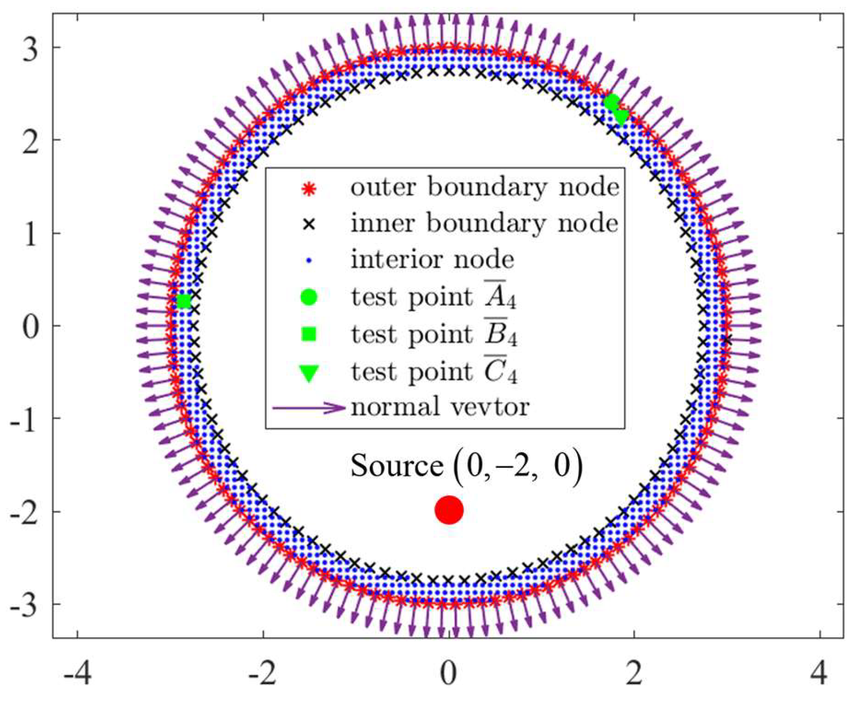
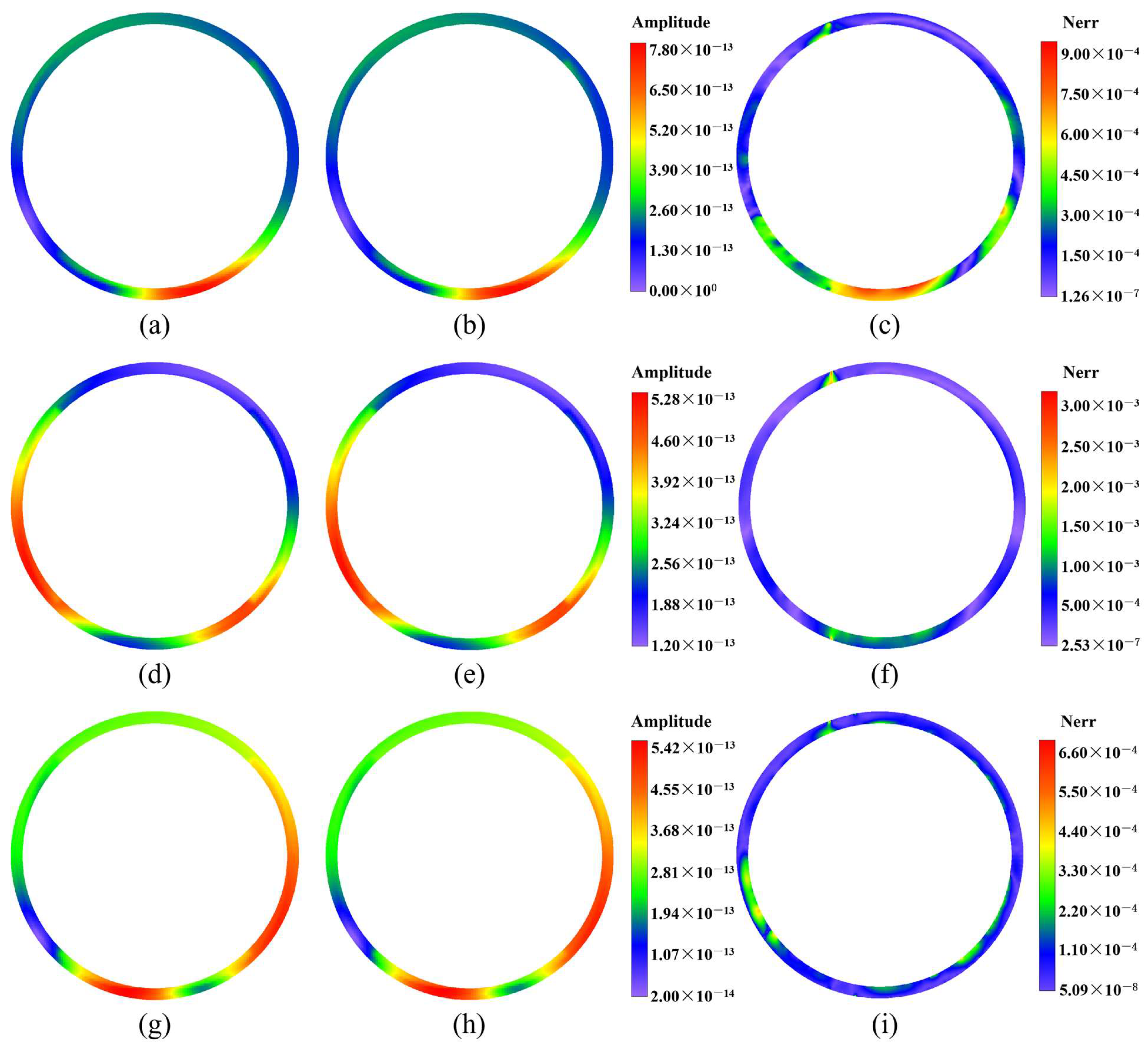
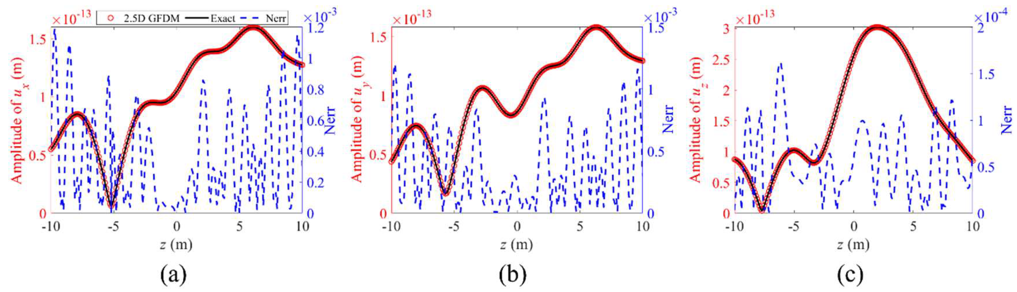
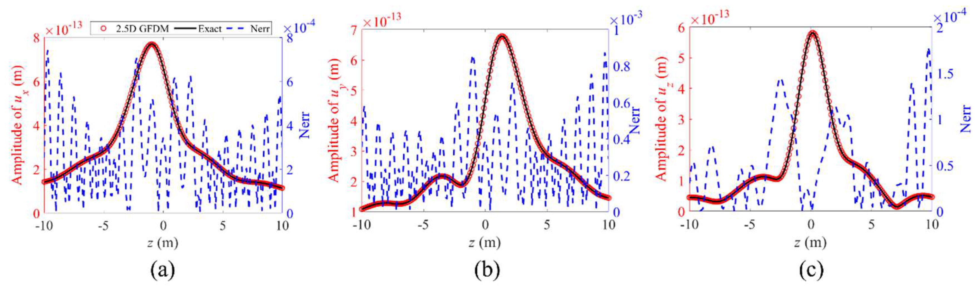
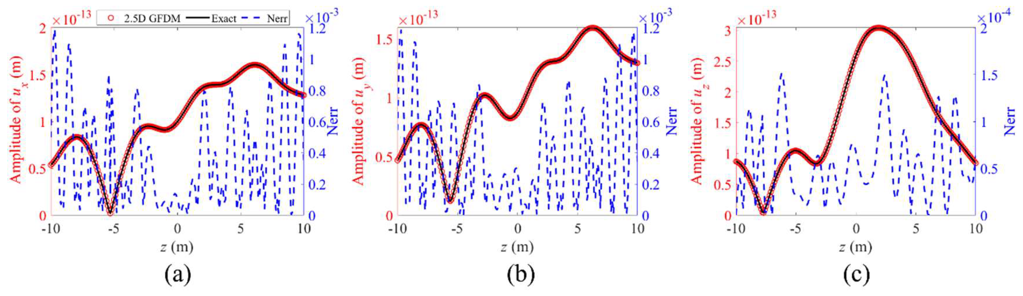
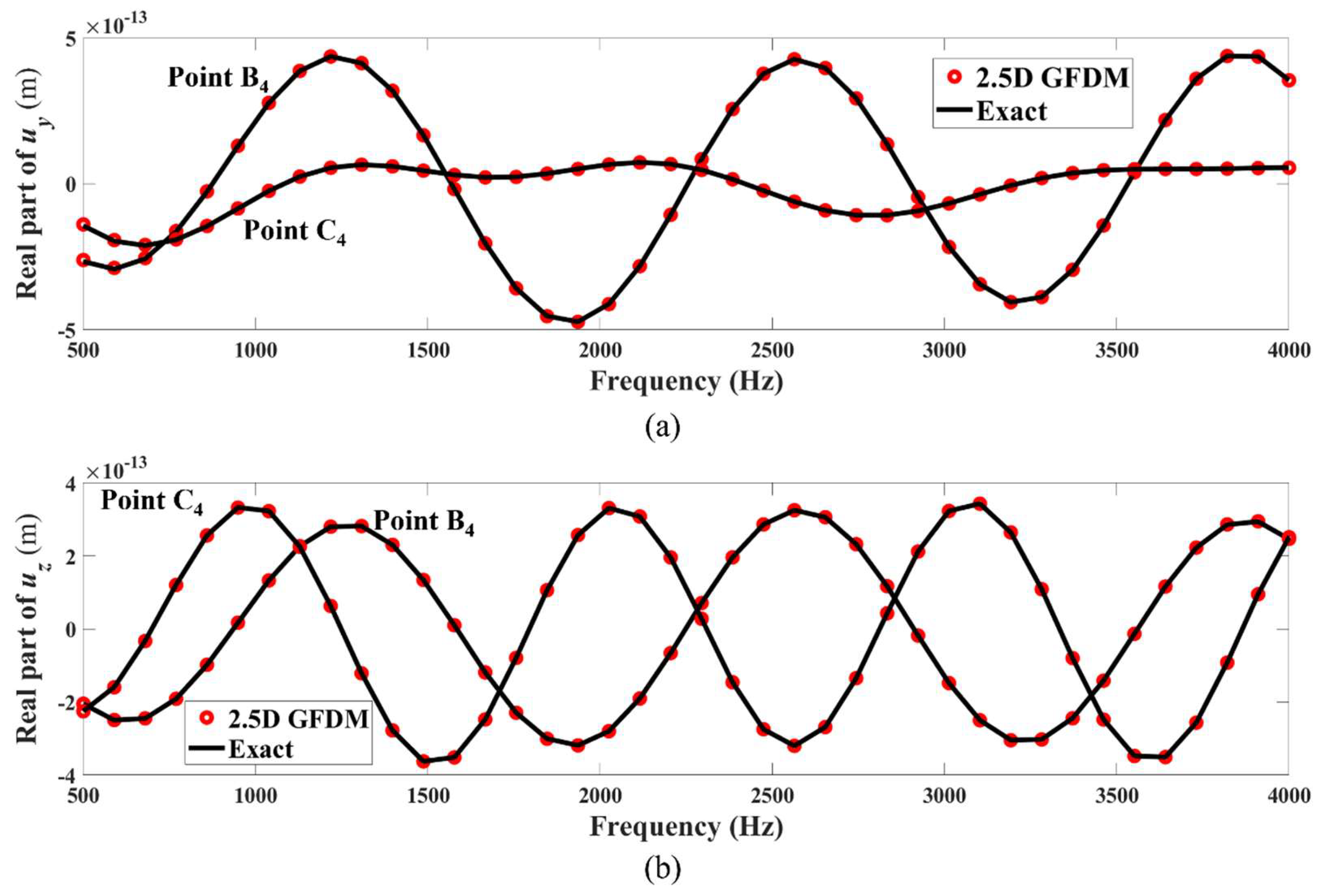
4. Numerical Examples

In this section, to evaluate the performance of the proposed 2.5D GFDM, elastic wave problems with three different domains are analyzed. For all examples consisting of longitudinally invariant medium, the mechanical properties of the material correspond to a Young Modulus $E$ of $156\times {10}^9\mathrm{Pa}$, a Poisson coefficient $\nu$ of 0.3, and a density $\rho$ of $2500{\mathrm{kg}/\mathrm{m}}^3$. The 3D approximations obtained using the 2.5D GFDM are contrasted with the exact solutions obtained from Green’s functions for displacement in the three-dimensional frequency domain. The requisite Green’s functions for various directionalities, as delineated by Lin [70], can be succinctly outlined as follows:

$$G_{xx}=A-B{\gamma }_x^2,$$

(40)

$$G_{yy}=A-B{\gamma }_y^2,$$

(41)

$$G_{zz}=A-B{\gamma }_z^2,$$

(42)

$$G_{xy}=G_{yx}=-B{\gamma }_x{\gamma }_y,$$

(43)

$$G_{xz}=G_{zx}=-B{\gamma }_x{\gamma }_z,$$

(44)

$$G_{yz}=G_{zy}=-B{\gamma }_y{\gamma }_z,$$

(45)

where

$$A={\displaystyle \frac{1}{4\pi {\omega }^2\rho }}\left(k_s^2{\displaystyle \frac{e^{-\mathrm{i}{k}_{s}r}}{r}}-\left(\mathrm{i}{k}_s+{\displaystyle \frac{1}{r}}\right){\displaystyle \frac{e^{-\mathrm{i}{k}_{s}r}}{r^2}}+\left(\mathrm{i}{k}_p+{\displaystyle \frac{1}{r}}\right){\displaystyle \frac{e^{-\mathrm{i}{k}_{p}r}}{r^2}}\right),$$

(46)

$$B={\displaystyle \frac{1}{4\pi {\omega }^2\rho }}\left(\left(k_s^2-{\displaystyle \frac{3}{r^2}}-{\displaystyle \frac{3\mathrm{i}{k}_s}{r}}\right){\displaystyle \frac{e^{-\mathrm{i}{k}_{s}r}}{r}}-\left(k_p^2-{\displaystyle \frac{3}{r^2}}-{\displaystyle \frac{3\mathrm{i}{k}_p}{r}}\right){\displaystyle \frac{e^{-\mathrm{i}{k}_{p}r}}{r}}\right),$$

(47)

in which $k_s=\sqrt{{\omega }^2\rho /\mu },$ $k_p=\sqrt{{\omega }^2\rho /\left(\lambda +2\mu \right)},$ ${\gamma }_j=\partial r/\partial x_j=x_j/r$ with $j=x,y,z,$ and $r$ stands for the three-dimensional distance between the source and field points. A point source is located at $\left(x_s,y_s,z_s\right)$. The analytical solutions of the problem in the frequency-wavenumber domain can be expressed in the subsequent format:

$${\overline{u}}_x=G_{xx}+G_{xy}+G_{xz},$$

(48)

$${\overline{u}}_y=G_{yx}+G_{yy}+G_{yz},$$

(49)

$${\overline{u}}_z=G_{zx}+G_{zy}+G_{zz}.$$

(50)

Furthermore, to assess the precision of the proposed methodology, the global error (Gerr) and the normalized error (Nerr) serve as pivotal metrics, employed as follows:

$$\mathrm{Gerr}(\varphi )=\sqrt{{\displaystyle \frac{{\displaystyle \sum _{i=1}^N{\left[{\varphi }_e\left(X_i\right)-{\varphi }_n\left(X_i\right)\right]}^2}}{{\displaystyle \sum _{i=1}^N{\left[{\varphi }_e\left(X_i\right)\right]}^2}}}},$$

(51)

$$\mathrm{Nerr}\left[{\varphi }_n\left(X_i\right)\right]={\displaystyle \frac{\left|{\varphi }_e\left(X_i\right)-{\varphi }_n\left(X_i\right)\right|}{\underset{x\in \Omega }{\max }\left|{\varphi }_e\left(X_i\right)\right|}},$$

(52)

where the variable $X_i$ denotes the $i^{th}$ calculation point, while $N$ represents the total count of calculation points, ${\varphi }_e\left(X_i\right)$ and ${\varphi }_n\left(X_i\right)$ correspond to the exact and numerical outcomes, respectively, at the $i^{th}$ calculation point.

Example 1. 

We first consider a three-dimensional model that is infinitely extended in the z-direction, featuring a square cross-section, covering 0 ≤ x, y ≤ 1. The geometry and parameters are invariant along the z-axis, as shown in Figure 2.

The interior nodes are uniformly distributed within the computational domain, and the same applies to the boundary nodes, as illustrated in Figure 3. The Dirichlet boundary conditions shown as Equation (6) are applied to the four edges of the square cross-section, where ${\mathbf{u}}_b$ is a vector comprising the components ${\overline{u}}_x$, ${\overline{u}}_y$, and ${\overline{u}}_z$. The boundary conditions will be transformed into 2.5D Dirichlet boundary conditions applicable to Equation (20) by performing the spatial Fourier transforms along the z-direction. In this case, the value of m is set to 12. The points source is located at $\left(-1.5,-1.5,0\right)$, oscillating with a frequency of f.

Before solving three-dimensional problems, it is essential to verify the applicability of the GFDM prior to applying the inverse spatial Fourier transform to the frequency-wavenumber domain results. The test point A₁ located at $\left(0.21,0.31\right)$ is selected to assess the accuracy of GFDM in the frequency-wavenumber domain. Figure 4 presents the real and imaginary parts of the displacement at the test point and the normalized error (Nerr) between numerical solutions and analytical solutions at the frequency of $1500\mathrm{Hz}$. This analysis covers a wavenumber range from $-10\mathrm{rad}/\mathrm{m}$ to $10\mathrm{rad}/\mathrm{m}$, sampled at linearly spaced intervals with increased density near $\pm k_p$ and $\pm k_s$, encompassing a total of 2704 points, including 204 boundary points and 2500 interior points. The analytical solutions of this problem can be expressed by

$$u_x^{2.5D}={\displaystyle \frac{1}{4\mathrm{i}\rho {\omega }^2}}\left[k_s^2{H}_{0\beta }-{\displaystyle \frac{1}{r_{2D}}}{B}_1+{\eta }_x^2{B}_2+{\eta }_x{\eta }_y{B}_2+\mathrm{i}{k}_z{\eta }_x{B}_1\right],$$

(53)

$$u_y^{2.5D}={\displaystyle \frac{1}{4\mathrm{i}\rho {\omega }^2}}\left[k_s^2{H}_{0\beta }-{\displaystyle \frac{1}{r_{2D}}}{B}_1+{\eta }_y^2{B}_2+{\eta }_x{\eta }_y{B}_2+\mathrm{i}{k}_z{\eta }_y{B}_1\right],$$

(54)

$$u_z^{2.5D}={\displaystyle \frac{1}{4\mathrm{i}\rho {\omega }^2}}\left[k_s^2{H}_{0\beta }-k_z^2{B}_0+\mathrm{i}{k}_z{\eta }_x{B}_1+\mathrm{i}{k}_z{\eta }_y{B}_1\right],$$

(55)

with $B_n=k_{\beta }^n{H}_{n\beta }-k_{\alpha }^n{H}_{n\alpha }$, $k_{\alpha }=\sqrt{k_p^2-k_z^2}$ with $\mathrm{Im}(k_{\alpha })<0$, $k_{\beta }=\sqrt{k_s^2-k_z^2}$ with $\mathrm{Im}(k_{\beta })<0$, ${\eta }_I=\partial r_{2D}/\partial x_I=x_I/r_{2D}$ with $I=x,y$, $H_{n\alpha }=H_n^{\left(2\right)}\left(k_{\alpha }{r}_{2D}\right)$, $H_{n\beta }=H_n^{\left(2\right)}\left(k_{\beta }{r}_{2D}\right)$, where the function $H_n^{\left(2\right)}$ represents the Hankel function of the second kind and of the $n^{th}$ order, while $r_{2D}$ denotes the two-dimensional distance between the source and the field points.

It can be observed that in the frequency-wavenumber domain, the numerical solutions obtained from the GFDM for displacements in three directions align well with the exact solutions. Consequently, the GFDM is capable of effectively addressing the propagation of elastic waves in the frequency-wavenumber domain.

To demonstrate the distinctive features of GFDM, the above problem was analyzed using non-uniformly distributed interior nodes and boundary nodes, as shown in Figure 5, specifically showcasing an instance of randomly arranged nodal points. Under identical parametric configurations, Figure 6 presents the real and imaginary parts of the displacement at the test point and Nerr between numerical solutions and analytical solutions with randomly distributed interior nodes and boundary nodes.

Comparative analysis of Figure 4 and Figure 6 reveals that while non-uniform nodal configurations induce a marginal elevation in normalized errors relative to uniform distributions, the accuracy remains acceptable.

In order to ascertain the integration limits for the inverse Fourier transform, the numerical results of the exact solution $u_y^{2.5D}$ are obtained by assigning values to the magnitude of $k_z$. Due to the presence of the Hankel function, $u_y^{2.5D}$ begins to decay rapidly at $\left|k_z\right|=k_s$. Specifically, when $k_z=-k_s$, $u_y^{2.5D}$ takes the value of $1.46\times {10}^{-14}-4.99\times {10}^{-13}\mathrm{i}$; when $k_z=k_s$, it takes the value of $3.97\times {10}^{-13}-7.96\times {10}^{-13}\mathrm{i}$. As $k_z$ is further extended to $-3k_s$ and $3k_s$, $u_y^{2.5D}$ exhibits a monotonic decrease to $1.82\times {10}^{-17}+5.43\times {10}^{-17}\mathrm{i}$. To achieve a balance between precision and efficiency, the integration limits were judiciously defined as $\left[-\gamma k_s,\gamma k_s\right]$, with $\gamma$ set to 4. Subsequent to performing the inverse Fourier transform on $u_y^{2.5D}$, the relative error between the computed outcome and ${\overline{u}}_y$ was meticulously calculated to be $2.16\times {10}^{-4}$, representing that the computational error associated with the chosen integration limits is adequate to satisfy the precision demands for subsequent computational analyses.

After applying an inverse spatial Fourier transform along the z-direction to the results in the frequency-wavenumber domain, we can obtain the 3D numerical solution for Example 1. Figure 7 shows the global error for the amplitude of three-dimensional displacements $u_z$, obtained from 2.5D GFDM, at different frequencies with respect to the total number of nodes. As it is illustrated in Figure 7, the 2.5D GFDM demonstrates stable convergence to the exact solutions.

Table 1. Global errors for $u_z$ obtained from different node distributions under varying numbers of nodes at 3000 Hz.

Number of Nodes	Global Errors
	Uniform Distribution	Non-Uniform Distribution
1020	2.3220 × 10−4	3.1495 × 10−4
1365	1.5837 × 10−4	1.9652 × 10−4
1760	1.1066 × 10−4	1.5055 × 10−4

presents the global errors for the amplitude of three-dimensional displacements $u_z$ obtained from different node distributions of 2.5D GFDM under varying numbers of nodes at 3000 Hz. Through comparative analysis, as the number of nodes increases, the errors generated by random node distribution converge with those from uniform distribution, demonstrating the robustness of 2.5D GFDM while indicating that stochastic nodal arrangements exert no significant influence on computational outcomes.

Table 2. Global errors and time costs for $u_z$ with varying m-values under 2704 nodes.

Frequency	Number of m	Global Errors	Time
3000 Hz	12	3.3319 × 10−4	316 s
	18	4.0470 × 10−4	330 s
	25	6.0844 × 10−4	342 s
4000 Hz	12	1.2688 × 10−3	320 s
	18	1.6112 × 10−3	331 s
	25	2.4420 × 10−3	358 s

presents the influence of different values of m (with a fixed node count of 2704) on the results of 2.5D GFDM at 3000 Hz and 4000 Hz. The data demonstrate that the numerical accuracy of the 2.5D GFDM exhibits low sensitivity to the variation of m-values. Notably, for a given number of nodes, arbitrarily increasing the values of m was found to adversely affect computational precision. Based on these findings, m = 12 was adopted for all subsequent analyses to balance efficiency and accuracy.

To validate the efficiency of the 2.5D GFDM method at the frequencies of 3000 Hz and 4000 Hz, we calculated the amplitude of 3D displacements $u_z$ on the $xy$ plane at $z=0\mathrm{m}$ using the 2.5D GFDM, recorded the computation time, and evaluated the global errors between the 2.5D GFDM results and the exact solution. The computation time and global error were then compared with those obtained from the 3D FEM combined with Perfectly Matched Layer (PML) in COMSOL Multiphysics^® 6.3, as shown in

Table 3. Global errors and computation time for $u_z$ obtained from 2.5D GFDM and 3D FEM-PML.

Frequency	2.5D GFDM			3D FEM-PML
	Number of Nodes	Global Errors	Time	Number of Units	Global Errors	Time
3000 Hz	1020	8.9959 × 10−4	46 s	187,322	2.4157 × 10−3	52 s
4000 Hz	2205	1.5428 × 10−4	243 s	784,280	5.7978 × 10−2	378 s

. The results demonstrate that the 2.5D GFDM outperforms traditional 3D numerical methods in both efficiency and accuracy.

In the following, to investigate the performance of the proposed method in calculating the $xy$ plane, we selected the plane at $z=5\mathrm{m}$ for frequencies of $2500\mathrm{Hz}$ and $3250\mathrm{Hz}$, another plane at $z=2\mathrm{m}$ for a frequency of $4000\mathrm{Hz}$, respectively. The normalized errors of these three cases are illustrated in Figure 8, Figure 9 and Figure 10. It can be observed that the 2.5D GFDM maintains a high level of accuracy when calculating the three-dimensional displacement fields on the $xy$ planes at various positions along the z-axis. Furthermore, the proposed method demonstrates higher accuracy in calculating the displacement fields $u_x$ and $u_y$ at lower frequencies.

Furthermore, we study the performance of the proposed method in calculating the propagation of displacements along the z-axis. In Example 1, we selected three test points located at B₁(0.05, 0.07), C₁(0.87, 0.69), and D₁(0.45, 0.89) within the computational domain, as shown in Figure 3, examining the propagation of displacement from $-10\mathrm{m}$ to $10\mathrm{m}$ along the z-axis at a frequency of $4000\mathrm{Hz}$. Figure 11, Figure 12 and Figure 13 illustrate the approximated solutions and exact solutions of $u_x$, $u_y$ and $u_z$ for this scenario, as well as their normalized errors, which demonstrate that the proposed method exhibits commendable accuracy in the computation of elastic wave propagation along the z-axis within the medium at higher frequencies.

Example 2. 

In this example, we consider a cylindrical model that is infinitely extended in the z-direction with a circular cross-section, where the circle is centered at the origin point (0, 0, 0) with a radius of 1 m, as depicted in Figure 14. The three-dimensional model parameters remain constant along the z-direction with the same point source as Example 1.

A total of 2116 nodes, including 148 boundary nodes and 1968 interior nodes, are uniformly distributed across both the interior and the boundary of the domain, as shown in Figure 15 (not to scale). Mixed boundary conditions are applied at the boundary nodes. For the upper half of the model’s boundary, Dirichlet boundary conditions are applied, whereas Neumann boundary conditions are imposed on the lower half of the boundary. ${\mathbf{t}}_b$ is a vector comprising the three components of traction. It is necessary to perform the spatial Fourier transforms along the z-direction on both Dirichlet boundary conditions and Neumann boundary conditions to derive their 2.5D form applicable to this example. The three-dimensional numerical solutions derived from the 2.5D GFDM are compared with the exact solutions given by Equations (48)–(50).

The performance of the proposed method is explored in calculating this example. Figure 16 depicts contour plots of the amplitude of displacement fields on the $xy$ plane $z=2\mathrm{m}$ for the problem at the frequency of $2500\mathrm{Hz}$. The upper part of the figure represents the computational results obtained utilizing the 2.5D GFDM introduced in this research. These results are compared with those on the lower part, which exhibits the displacement fields derived from the exact analytical solutions. It is apparent that there is an exact correspondence between the two parts of the figures.

Moreover, Figure 17 and Figure 18 display color maps calculated under conditions analogous to those in Figure 16, but for the $xy$ planes of $z=0.5\mathrm{m}$ and $z=1\mathrm{m}$ with excitation frequencies of $3250\mathrm{Hz}$ and $4000\mathrm{Hz}$, respectively. Consistent with the previous figure, a precise correspondence is observed between the outcomes yielded by the numerical method and exact solutions.

In the following, the accuracy of the method in calculating the propagation of displacements along the z-axis is assessed with respect to its application to Example 2. Figure 19, Figure 20 and Figure 21 exhibit the propagation of displacement in three directions and the normalized errors between the approximated solutions and the exact solutions of three test points from $-10\mathrm{m}$ to $10\mathrm{m}$ along the z-direction with a source frequency of $2250\mathrm{Hz}$. The test points are selected at ${\overline{\mathrm{A}}}_2$ (−0.3, −0.5), ${\overline{\mathrm{B}}}_2$ (−0.82, 0.42), and ${\overline{\mathrm{C}}}_2$ (0.58, 0.58), as shown in Figure 15, within the computational domain. From the figures, it can be observed that the normalized error primarily maintains an amplitude around 10⁻⁴, once again demonstrating that this method retains robustness when calculating the propagation of displacement in the z-direction, which indicates that this method is capable of accurately predicting the displacement fields at the frequency for this example.

In Figure 22 and Figure 23, the real and imaginary parts of displacements $u_y$ and $u_z$ against the frequencies ranging from $500$ to $4000\mathrm{Hz}$, as derived from both 2.5D GFDM and exact solutions at the receiving points B₂(−0.82, 0.42, 1) and C₂(0.58, 0.58, 1), are depicted. A close correspondence between the outcomes of the proposed method and analytical solutions at the considered frequencies can be evidently observed.

Example 3. 

To further validate the performance of the method related to engineering applications, a tunnel structure infinitely extended in the z-direction with an annular cross-section, centered at the origin, is examined, where the external radius is 3.0 m and the inner radius is 2.75 m, with a medium of 0.25 m thickness filling the space between the two radii. The medium of the tunnel and its cross-sectional geometry remain constant along the z-direction, as illustrated in Figure 24.

The nodes, consisting of 180 inner boundary points, 197 outer boundary points, and 1832 interior nodes between them, are uniformly distributed across both the interior and the boundary of the domain, as shown in Figure 25. The Dirichlet boundary conditions shown as Equation (6) are imposed on the entire inner boundary of the tunnel, while Neumann boundary conditions are applied to the outer boundary. Consistent with Example 2, a spatial Fourier transform along the z-direction shall be performed on both boundary conditions to derive their 2.5D form applicable to this example. In the first case of Example 3, we consider a source point positioned outside the entire tunnel structure, specifically at $\left(0,-4,0\right)$.

Figure 26 presents contour plots illustrating the amplitude of the displacement field on the $xy$ plane at $z=3\mathrm{m}$ for the problem at the frequency of $2250\mathrm{Hz}$. The left-hand section of the figure shows the outcomes of calculations using the 2.5D GFDM. These outcomes are juxtaposed with the central section, which displays displacement fields derived from analytical solutions. The right-hand section of the figure provides contour plots of the normalized errors between the left and central sections. Additionally, in the map of normalized errors, it is observable that for the displacement fields in three directions, only a very small portion of the normalized errors is on the order of 10⁻³, while the remaining normalized errors are on the order of 10⁻⁴, demonstrating a high level of agreement. This indicates that the 2.5D GFDM is effective in computing displacement fields for tunnel structures with thinner walls. In addition, Figure 27 and Figure 28 exhibit chromatic representations computed under conditions parallel to those in Figure 26, yet for the planes at $z=5\mathrm{m}$ and $z=1\mathrm{m}$, with excitation frequencies of 3250 Hz and 4000 Hz, respectively. Aligning with the preceding figure, a congruence is discerned between the numerical outcomes and the analytical solutions. It should be noted that the regions with higher errors in the map of normalized errors are results of the differences in the distribution of grid points between the computational domain and the boundaries during the discretization process.

Next, the propagation of displacement in three directions and the corresponding normalized errors for three test points, ranging from −10 m to 10 m along the z-direction as shown in Figure 29, Figure 30 and Figure 31, are explored, with the source point oscillating at the frequency of $2250\mathrm{Hz}$. The test points, as shown in Figure 25, designated as ${\overline{\mathrm{A}}}_3$ (−1.51, −2.50), ${\overline{\mathrm{B}}}_3$ (2.85, 0), and ${\overline{\mathrm{C}}}_3$ (2.26, 1.76), are located within the computational domain. Analysis of the figures reveals that the majority of normalized errors lie within the order of 10⁻⁴, thereby reaffirming the high accuracy of this method. This reiterates the method’s capability to accurately predict the response at the specified frequency for the tunnel structure affected by an external source point.

In Figure 32 and Figure 33, the real and imaginary components of the displacements $u_y$ and $u_z$ as determined at the receiving points ${\mathrm{B}}_3$ (2.85, 0, 1) and ${\mathrm{C}}_3$ (2.26, 1.76, 1) over a frequency range of 500 to $4000\mathrm{Hz}$ using both the 2.5D GFDM and exact solutions are illustrated. Again, the figures demonstrate a strong correlation between the outcomes yielded by the proposed method and the analytical solutions at the specified frequencies. This reaffirms that the 2.5D GFDM demonstrates a significant level of accuracy in calculating the frequency response of tunnel-like structures with thinner walls when subjected to the influence of an external point source.

In the subsequent illustrative case, we delve into the performance of 2.5D GFDM within the context of computational engineering models. Specifically, we situate the source point within the confines of a tunnel structure, designated at the coordinates (0, −2, 0), to emulate a simplified representation of a vibration source attributable to an underground train, as shown in Figure 34. The remaining parameters for this case are aligned with the conditions outlined in the first case of Example 3.

Figure 35, Figure 36 and Figure 37 display the contour plots of the displacement amplitude on the $xy$ plane at $z=2\mathrm{m}$, which is influenced by a point source situated at coordinates (0, −2, 0), for a frequency of $2250\mathrm{Hz}$. Consistent with the first case of Example 3, the left section of the figures illustrates the computational results from the 2.5D GFDM. These results are contrasted with the central section, which portrays the displacement fields obtained from rigorous analytical solutions. The right section presents the contour plots of the normalized errors between the computational and analytical results. It is evident from the map of normalized errors that for the displacements in three dimensions, the error distribution remains predominantly within the order of magnitude of 10⁻⁴ along most of the z-axis, indicating a substantial degree of concordance. Additionally, Figure 35 and Figure 36 present contour plots analogous to those in Figure 33, but for different planes at $z=5\mathrm{m}$ and $z=1\mathrm{m}$, with corresponding excitation frequencies of $3250\mathrm{Hz}$ and $4000\mathrm{Hz}$, respectively. These figures, again, demonstrate a correlation between the numerical model’s predictions and the accurate analytical results, echoing the findings from the earlier figures. Analogous to the first case in Example 3, the minor error oscillations in certain areas of the displacement fields across three directions, as shown in the figures, are caused by the distribution discrepancy between the computational interior nodes and boundary nodes. These fluctuations, including those mentioned in the previous examples, however, do not compromise the method’s accuracy.

Subsequently, this investigation delves into the propagation of displacement and the corresponding normalized errors in three directions for three test points along the z-axis, ranging from −10 m to 10 m, with the source point oscillating at a frequency of 2250 Hz, as shown in Figure 38, Figure 39 and Figure 40. The test points, designated as ${\overline{\mathrm{A}}}_4$ (1.76, 2.41), ${\overline{\mathrm{B}}}_4$ (−2.85, 0.27), and ${\overline{\mathrm{C}}}_4$ (1.86, 2.26), are positioned within the computational domain. A meticulous review of the graphical data reveals that the normalized errors generally lie within 10⁻⁴, except for a few localized peaks, thereby confirming the high accuracy of this method in ascertaining the propagation of displacement in the z-direction. This further underscores the capability of 2.5D GFDM not only to accurately predict the response of the tunnel structure affected by an external point source at the specified frequency but also to demonstrate good accuracy in forecasting the vibrations of the tunnel structure caused by internal vibration sources.

Figure 40, Figure 41 and Figure 42 present the real and imaginary parts of displacement components at points B₄(−2.85, 0.27, 1) and C₄(1.86, 2.26, 1) over a frequency range of 500 to 4000 $\mathrm{Hz}$, with results obtained through both the 2.5D GFDM and exact solutions. The strong agreement between the proposed method and the analytical solutions can be evidently observed, which confirms the reliability of the 2.5D GFDM. This highlights its capability to accurately predict the frequency response of the tunnel structure caused by internal vibration sources within the tunnel. In the second case of Example 3, the collective findings from the research affirm the efficacy of the method in question. This high level of consistency between 2.5D GFDM and exact solutions suggests that the 2.5D GFDM demonstrates potential in predicting the responses of tunnel structures to vibrations induced by underground railway trains.

5. Conclusions

This paper presents a method that combines 2.5D technology with the GFDM to solve the three-dimensional elastic wave propagation problem with an invariant cross-section in a certain direction. By employing the spatial Fourier transform, the complex three-dimensional problem is transformed into a more computationally convenient two-dimensional problem in the frequency-wavenumber domain. The resulting two-dimensional problem is then solved using the novel mesh-free numerical method GFDM, and the obtained solutions in the frequency-wave number domain are converted back into three-dimensional numerical solutions through the inverse Fourier transform. To investigate the performance of this method, three numerical examples were selected, and the numerical solutions of each example, including two cases in Example 3, were thoroughly compared with their corresponding exact solutions.

In Example 1, the two-dimensional numerical solutions in the frequency-wave number domain demonstrate the accuracy of the mesh-free numerical algorithm GFDM. Based on this, the three-dimensional numerical solutions obtained through the inverse Fourier transform, whether for the displacement field on the $xy$ planes or the displacement response in the z-direction, show the considerable accuracy and stability of the 2.5D GFDM. Example 2 demonstrates that the 2.5D GFDM not only calculates the displacement field on $xy$ planes and the displacement response in the z-direction but also demonstrates high precision in calculating the frequency response at each point. Example 3 indicates that the 2.5D GFDM can calculate engineering problems such as the impact of vibrations caused by subway trains on tunnel structures and also shows its excellent computational capability.

Given that this study primarily focuses on developing novel methodologies for addressing elastic wave propagation in axially infinite-extended structures, with a particular focus on underground engineering applications such as vibration wave propagation in tunnels, further research is required to determine whether the 2.5D GFDM (Generalized Finite Difference Method) can be extended to handle cross-sections with higher geometric complexity (e.g., star-shaped or gear-shaped profiles). Key challenges needing in-depth investigation include (i) the strategic placement of calculation points in regions with highly complex geometries and (ii) potential hybrid/coupling approaches with other 2.5D numerical methods to enable simulations of more intricate geometries. The applicability of the 2.5D methodology is constrained by two principal factors: First, the approach inherently requires invariance in both cross-sectional configuration and material properties of the medium along the axial extension direction, thereby precluding its implementation in scenarios involving geometric or material heterogeneity in the longitudinal dimension. Second, stringent geometric scaling criteria must be satisfied, specifically that the model’s longitudinal dimension should significantly exceed the characteristic wavelength to effectively mitigate boundary-induced elastic wave reflections, a critical prerequisite for maintaining numerical precision in semi-analytical simulation frameworks. Failing that, such issues necessitate the application of conventional 3D methodologies to achieve effective resolution.

In summary, the proposed 2.5D GFDM can solve the three-dimensional elastic wave propagation problem with an invariant cross-section, including practical engineering problems. More complex engineering problems, such as the impact of vibrations caused by subway rail transit on the ground, are still under study and will be presented in subsequent articles.

References

1. Bao, H.; Bielak, J.; Ghattas, O.; Kallivokas, L.F.; O’Hallaron, D.R.; Shewchuk, J.R.; Xu, J. Large-scale simulation of elastic wave propagation in heterogeneous media on parallel computers. Comput. Methods Appl. Mech. Eng. 1998, 152, 85–102. [Google Scholar] [CrossRef]
2. Ureña, F.; Benito, J.J.; Salete, E.; Gavete, L. A note on the application of the generalized finite difference method to seismic wave propagation in 2D. J. Comput. Appl. Math. 2012, 236, 3016–3025. [Google Scholar] [CrossRef]
3. Benito, J.; Ureña, F.; Salete, E.; Muelas, A.; Gavete, L.; Galindo, R. Wave propagation in soils problems using the Generalized Finite Difference Method. Soil Dyn. Earthq. Eng. 2015, 79, 190–198. [Google Scholar] [CrossRef]
4. Salete, E.; Benito, J.J.; Ureña, F.; Gavete, L.; Ureña, M.; García, A. Stability of perfectly matched layer regions in generalized finite difference method for wave problems. J. Comput. Appl. Math. 2017, 312, 231–239. [Google Scholar] [CrossRef]
5. Qu, W.; Gu, Y.; Fan, C.-M. A stable numerical framework for long-time dynamic crack analysis. Int. J. Solids Struct. 2024, 293, 112768. [Google Scholar] [CrossRef]
6. Moser, F.; Jacobs, L.J.; Qu, J. Modeling elastic wave propagation in waveguides with the finite element method. Ndt E Int. 1999, 32, 225–234. [Google Scholar] [CrossRef]
7. Serón, F.; Sanz, F.; Kindelan, M.; Badal, J. Finite-element method for elastic wave propagation. Commun. Appl. Numer. Methods 1990, 6, 359–368. [Google Scholar] [CrossRef]
8. Fu, Z.; Xi, Q.; Li, Y.; Huang, H.; Rabczuk, T. Hybrid FEM–SBM solver for structural vibration induced underwater acoustic radiation in shallow marine environment. Comput. Methods Appl. Mech. Eng. 2020, 369, 113236. [Google Scholar] [CrossRef]
9. Li, Y.; Dang, S.; Li, W.; Chai, Y. Free and forced vibration analysis of two-dimensional linear elastic solids using the finite element methods enriched by interpolation cover functions. Mathematics 2022, 10, 456. [Google Scholar] [CrossRef]
10. Jianfeng, Z. Quadrangle-grid velocity-stress finite-difference method for elastic-wave-propagation simulation. Geophys. J. Int. 1997, 131, 127–134. [Google Scholar] [CrossRef]
11. Zhang, W.; Zhang, Z.; Chen, X. Three-dimensional elastic wave numerical modelling in the presence of surface topography by a collocated-grid finite-difference method on curvilinear grids. Geophys. J. Int. 2012, 190, 358–378. [Google Scholar] [CrossRef]
12. Beskos, D.E. Boundary element methods in dynamic analysis. Appl. Mech. Rev. 1987, 40, 1–23. [Google Scholar] [CrossRef]
13. Liu, Y.; Rizzo, F. Hypersingular boundary integral equations for radiation and scattering of elastic waves in three dimensions. Comput. Methods Appl. Mech. Eng. 1993, 107, 131–144. [Google Scholar] [CrossRef]
14. Zou, M.-s.; Wu, Y.-s.; Liu, Y.-m.; Lin, C.-g. A three-dimensional hydroelasticity theory for ship structures in acoustic field of shallow sea. J. Hydrodyn. Ser. B 2013, 25, 929–937. [Google Scholar] [CrossRef]
15. Liu, Z.; Liu, L.; Liang, J.; Zhou, Y. An indirect boundary element method to model the 3-D scattering of elastic waves in a fluid-saturated poroelastic half-space. Eng. Anal. Bound. Elem. 2016, 66, 91–108. [Google Scholar] [CrossRef]
16. Perrey-Debain, E.; Trevelyan, J.; Bettess, P. Plane wave interpolation in direct collocation boundary element method for radiation and wave scattering: Numerical aspects and applications. J. Sound Vib. 2003, 261, 839–858. [Google Scholar] [CrossRef]
17. De Basabe, J.D.; Sen, M.K. A comparison of finite-difference and spectral-element methods for elastic wave propagation in media with a fluid-solid interface. Geophys. J. Int. 2015, 200, 278–298. [Google Scholar] [CrossRef]
18. Deckers, E.; Jonckheere, S.; Van Belle, L.; Claeys, C.; Desmet, W. Prediction of transmission, reflection and absorption coefficients of periodic structures using a hybrid wave based–finite element unit cell method. J. Comput. Phys. 2018, 356, 282–302. [Google Scholar] [CrossRef]
19. Moldovan, I.D.; de Freitas, J.A.T. Hybrid-Trefftz finite element models for bounded and unbounded elastodynamic problems. In Proceedings of III European Conference on Computational Mechanics: Solids, Structures and Coupled Problems in Engineering: Book of Abstracts; Springer: Dordrecht, The Netherlands, 2006; p. 400. [Google Scholar]
20. de Freitas, J.T. Hybrid finite element formulations for elastodynamic analysis in the frequency domain. Int. J. Solids Struct. 1999, 36, 1883–1923. [Google Scholar] [CrossRef]
21. Qin, Q.-H. Trefftz Finite Element Method and Its Applications. Appl. Mech. Rev. 2005, 58, 316–337. [Google Scholar] [CrossRef]
22. Fu, Z.-J.; Xi, Q.; Gu, Y.; Li, J.; Qu, W.; Sun, L.; Wei, X.; Wang, F.; Lin, J.; Li, W.; et al. Singular boundary method: A review and computer implementation aspects. Eng. Anal. Bound. Elem. 2023, 147, 231–266. [Google Scholar] [CrossRef]
23. Gu, Y.; Chen, W.; He, X.-Q. Singular boundary method for steady-state heat conduction in three dimensional general anisotropic media. Int. J. Heat Mass Transf. 2012, 55, 4837–4848. [Google Scholar] [CrossRef]
24. Liu, H.; Wang, F. A novel semi-analytical meshless method for the thickness optimization of porous material distributed on sound barriers. Appl. Math. Lett. 2024, 147, 108844. [Google Scholar] [CrossRef]
25. Wang, F.; Chen, W.; Tadeu, A.; Correia, C.G. Singular boundary method for transient convection–diffusion problems with time-dependent fundamental solution. Int. J. Heat Mass Transf. 2017, 114, 1126–1134. [Google Scholar] [CrossRef]
26. Liu, Q.; Šarler, B. Non-singular method of fundamental solutions for two-dimensional isotropic elasticity problems. Comput. Model. Eng. Sci. 2013, 91, 235–266. [Google Scholar]
27. Lan, L.; Zhou, Z.; Liu, H.; Wei, X.; Wang, F. An ACA-BM-SBM for 2D acoustic sensitivity analysis. AIMS Math. 2024, 9, 1939–1958. [Google Scholar] [CrossRef]
28. Fan, C.-M.; Chien, C.-S.; Chan, H.-F.; Chiu, C.-L. The local RBF collocation method for solving the double-diffusive natural convection in fluid-saturated porous media. Int. J. Heat Mass Transf. 2013, 57, 500–503. [Google Scholar] [CrossRef]
29. Fu, Z.-J.; Chen, W.; Yang, H.-T. Boundary particle method for Laplace transformed time fractional diffusion equations. J. Comput. Phys. 2013, 235, 52–66. [Google Scholar] [CrossRef]
30. Fan, C.; Liu, Y.; Chan, H.; Hsiao, S. Solutions of boundary detection problem for modified Helmholtz equation by Trefftz method. Inverse Probl. Sci. Eng. 2014, 22, 267–281. [Google Scholar] [CrossRef]
31. Liu, C.-S.; Kuo, C.-L.; Jhao, W.-S. The multiple-scale polynomial Trefftz method for solving inverse heat conduction problems. Int. J. Heat Mass Transf. 2016, 95, 936–943. [Google Scholar] [CrossRef]
32. Ju, B.; Gu, Y.; Wang, R. An enriched radial integration method for evaluating domain integrals in transient boundary element analysis. Appl. Math. Lett. 2024, 153, 109067. [Google Scholar] [CrossRef]
33. Wang, F.; Wang, C.; Chen, Z. Local knot method for 2D and 3D convection-diffusion-reaction equations in arbitrary domains. Appl. Math. Lett. 2020, 105, 106308. [Google Scholar] [CrossRef]
34. Qiu, X.; Yue, X. Solving time fractional partial differential equations with variable coefficients using a spatio-temporal meshless method. AIMS Math 2024, 9, 27150–27166. [Google Scholar] [CrossRef]
35. Chen, C.-S.; Fan, C.-M.; Wen, P. The method of approximate particular solutions for solving elliptic problems with variable coefficients. Int. J. Comput. Methods 2011, 8, 545–559. [Google Scholar] [CrossRef]
36. Chen, C.-S.; Fan, C.-M.; Wen, P. The method of approximate particular solutions for solving certain partial differential equations. Numer. Methods Partial Differ. Equ. 2012, 28, 506–522. [Google Scholar] [CrossRef]
37. Benito, J.; Urena, F.; Gavete, L. Influence of several factors in the generalized finite difference method. Appl. Math. Model. 2001, 25, 1039–1053. [Google Scholar] [CrossRef]
38. Gavete, L.; Gavete, M.; Benito, J. Improvements of generalized finite difference method and comparison with other meshless method. Appl. Math. Model. 2003, 27, 831–847. [Google Scholar] [CrossRef]
39. Prieto, F.U.; Muñoz, J.J.B.; Corvinos, L.G. Application of the generalized finite difference method to solve the advection–diffusion equation. J. Comput. Appl. Math. 2011, 235, 1849–1855. [Google Scholar] [CrossRef]
40. Chan, H.-F.; Fan, C.-M.; Kuo, C.-W. Generalized finite difference method for solving two-dimensional non-linear obstacle problems. Eng. Anal. Bound. Elem. 2013, 37, 1189–1196. [Google Scholar] [CrossRef]
41. Li, P.-W.; Fan, C.-M.; Chen, C.-Y.; Ku, C.-Y. Generalized finite difference method for numerical solutions of density-driven groundwater flows. Comput. Model. Eng. Sci. 2014, 101, 319–350. [Google Scholar]
42. Hosseini, S.M. Shock-induced two dimensional coupled non-Fickian diffusion–elasticity analysis using meshless generalized finite difference (GFD) method. Eng. Anal. Bound. Elem. 2015, 61, 232–240. [Google Scholar] [CrossRef]
43. Gavete, L.; Ureña, F.; Benito, J.J.; García, A.; Ureña, M.; Salete, E. Solving second order non-linear elliptic partial differential equations using generalized finite difference method. J. Comput. Appl. Math. 2017, 318, 378–387. [Google Scholar] [CrossRef]
44. Gu, Y.; Wang, L.; Chen, W.; Zhang, C.; He, X. Application of the meshless generalized finite difference method to inverse heat source problems. Int. J. Heat Mass Transf. 2017, 108, 721–729. [Google Scholar] [CrossRef]
45. Hua, Q.; Gu, Y.; Qu, W.; Chen, W.; Zhang, C. A meshless generalized finite difference method for inverse Cauchy problems associated with three-dimensional inhomogeneous Helmholtz-type equations. Eng. Anal. Bound. Elem. 2017, 82, 162–171. [Google Scholar] [CrossRef]
46. Sun, W.; Qu, W.; Gu, Y.; Zhao, S. Three-dimensional elastodynamic analysis employing the generalized finite difference method with arbitrary-order accuracy. Comput. Math. Appl. 2024, 174, 151–166. [Google Scholar] [CrossRef]
47. Zhang, F.; Li, P.-W.; Gu, Y.; Fan, C.-M. A space-time generalized finite difference scheme for long wave propagation based on high-order Korteweg-de Vries type equations. Math. Comput. Simul. 2025, 228, 298–312. [Google Scholar] [CrossRef]
48. Orkisz, J. Meshless finite difference method I. Basic approach. In Proceedings of the IACM-Fourth World Congress in Computational Mechanics, Buenos Aires, Argentina, 29 June–2 July 1998. [Google Scholar]
49. Li, P.-W.; Chen, W.; Fu, Z.-J.; Fan, C.-M. Generalized finite difference method for solving the double-diffusive natural convection in fluid-saturated porous media. Eng. Anal. Bound. Elem. 2018, 95, 175–186. [Google Scholar] [CrossRef]
50. Song, L.; Li, P.-W.; Gu, Y.; Fan, C.-M. Generalized finite difference method for solving stationary 2D and 3D Stokes equations with a mixed boundary condition. Comput. Math. Appl. 2020, 80, 1726–1743. [Google Scholar] [CrossRef]
51. Suchde, P.; Kuhnert, J. A meshfree generalized finite difference method for surface PDEs. Comput. Math. Appl. 2019, 78, 2789–2805. [Google Scholar] [CrossRef]
52. Ureña, F.; Salete, E.; Benito, J.J.; Gavete, L. Solving third-and fourth-order partial differential equations using GFDM: Application to solve problems of plates. Int. J. Comput. Math. 2012, 89, 366–376. [Google Scholar] [CrossRef]
53. Gu, Y.; Qu, W.; Chen, W.; Song, L.; Zhang, C. The generalized finite difference method for long-time dynamic modeling of three-dimensional coupled thermoelasticity problems. J. Comput. Phys. 2019, 384, 42–59. [Google Scholar] [CrossRef]
54. Ma, L.; Zhang, C.; Ouyang, H.; Yan, Q.; Yu, W. 2.5 D modelling of wave propagation in longitudinally curved viscoelastic structure using a coupled FEM-PML approach. Eng. Struct. 2021, 226, 111337. [Google Scholar] [CrossRef]
55. Sun, L.; Wei, X.; Chen, B. A meshless singular boundary method for elastic wave propagation in 2D partially saturated poroelastic media. Eng. Anal. Bound. Elem. 2020, 113, 82–98. [Google Scholar] [CrossRef]
56. Wei, X.; Liu, D.; Luo, W.; Chen, S.; Sun, L. A half-space singular boundary method for predicting ground-borne vibrations. Appl. Math. Model. 2022, 111, 630–643. [Google Scholar] [CrossRef]
57. Gu, Y.; Chen, W.; Fu, Z.-J.; Zhang, B. The singular boundary method: Mathematical background and application in orthotropic elastic problems. Eng. Anal. Bound. Elem. 2014, 44, 152–160. [Google Scholar] [CrossRef]
58. Liravi, H.; Arcos, R.; Clot, A.; Conto, K.F.; Romeu, J. A 2.5 D coupled FEM–SBM methodology for soil–structure dynamic interaction problems. Eng. Struct. 2022, 250, 113371. [Google Scholar] [CrossRef]
59. Liravi, H.; Clot, A.; Arcos, R.; Fakhraei, J.; Godinho, L.; Conto, K.F.; Romeu, J. A 2.5 D hybrid SBM-MFS methodology for elastic wave propagation problems. J. Sound Vib. 2024, 586, 118501. [Google Scholar] [CrossRef]
60. Sun, L.; Fu, Z.; Chen, Z. A localized collocation solver based on fundamental solutions for 3D time harmonic elastic wave propagation analysis. Appl. Math. Comput. 2023, 439, 127600. [Google Scholar] [CrossRef]
61. Aubry, D.; Clouteau, D.; Bonnet, G. Modelling of wave propagation due to fixed or mobile dynamic sources. In Proceedings of the Workshop Wave ’94, Wave Propagation and Reduction of Vibrations, Ruhr-Universität Bochum, Germany, 8 December 1994; pp. 109–121. [Google Scholar]
62. Sheng, X.; Jones, C.; Petyt, M. Ground vibration generated by a harmonic load acting on a railway track. J. Sound Vib. 1999, 225, 3–28. [Google Scholar] [CrossRef]
63. Sheng, X.-Z.; Jones, C.; Petyt, M. Ground vibration generated by a load moving along a railway track. J. Sound Vib. 1999, 228, 129–156. [Google Scholar] [CrossRef]
64. Zeng, S.; Chen, F.; Li, D.; Chen, J.; Chen, J. A novel 2.5 D finite difference scheme for simulations of resistivity logging in anisotropic media. J. Appl. Geophys. 2018, 150, 144–152. [Google Scholar] [CrossRef]
65. Suchde, P. Particle-based adaptive coupling of 3D and 2D fluid flow models. Comput. Methods Appl. Mech. Eng. 2024, 429, 117199. [Google Scholar] [CrossRef]
66. Yang, S.-b.; Zhou, B.; Bai, C.-y. A generalized 2.5-D time-domain seismic wave equation to accommodate various elastic media and boundary conditions. Pure Appl. Geophys. 2021, 178, 2999–3025. [Google Scholar] [CrossRef]
67. Amado-Mendes, P.; Costa, P.A.; Godinho, L.M.; Lopes, P. 2.5 D MFS–FEM model for the prediction of vibrations due to underground railway traffic. Eng. Struct. 2015, 104, 141–154. [Google Scholar] [CrossRef]
68. Tadeu, A.J.; Kausel, E. Green’s functions for two-and-a-half-dimensional elastodynamic problems. J. Eng. Mech. 2000, 126, 1093–1097. [Google Scholar] [CrossRef]
69. Xing, Y.; Song, L.; He, X.; Qiu, C. A generalized finite difference method for solving elliptic interface problems. Math. Comput. Simul. 2020, 178, 109–124. [Google Scholar] [CrossRef]
70. Lin, J.; Chen, W.; Sun, L. Simulation of elastic wave propagation in layered materials by the method of fundamental solutions. Eng. Anal. Bound. Elem. 2015, 57, 88–95. [Google Scholar] [CrossRef]
Figure 1. An irregular point cloud and the local GFDM star for a 2D case.
Mathematics 13 01249 g001
Figure 2. A three-dimensional model with a square cross-section and invariant geometry along the z-direction.
Mathematics 13 01249 g002
Figure 3. A schematic representation of uniform distribution of interior nodes and boundary nodes, along with a source point and test points for Example 1.
Mathematics 13 01249 g003
Figure 4. Solutions of displacements by the GFDM at the test point A1 with the frequency of 2500   Hz : (a,c,e) represent real parts of u ˜ x , u ˜ y , u ˜ z , respectively, and the normalized errors between numerical and analytical solutions; (b,d,f) represent imaginary parts of, u ˜ x   u ˜ y , u ˜ z , respectively, and the normalized errors between numerical and analytical solutions.
Mathematics 13 01249 g004
Figure 5. A schematic representation of non-uniform distribution of interior nodes and boundary nodes for Example 1.
Mathematics 13 01249 g005
Figure 6. Solutions of displacements by the GFDM, with non-uniformly distributed interior nodes and boundary nodes, at the test point A1 with the frequency of 2500   Hz : (a,c,e) represent real parts of u ˜ x , u ˜ y , u ˜ z , respectively, and the normalized errors between numerical and analytical solutions; (b,d,f) represent imaginary parts of, u ˜ x , u ˜ y , u ˜ z , respectively, and the normalized errors between numerical and analytical solutions.
Mathematics 13 01249 g006
Figure 7. Global errors for the amplitude of three-dimensional displacement u z at different frequencies of 3000   Hz , 4000   Hz and 5000   Hz with respect to the total number of nodes.
Mathematics 13 01249 g007
Figure 8. The normalized errors of the amplitude of displacement fields (a) u x , (b) u y , and (c) u z on the x y plane at z = 5   m for Example 1 with a frequency of 2500   Hz .
Mathematics 13 01249 g008
Figure 9. The normalized errors of the amplitude of displacement fields (a) u x , (b) u y , and (c) u z on the x y plane at z = 5   m for Example 1 with a frequency of 3250   Hz .
Mathematics 13 01249 g009
Figure 10. The normalized errors of the amplitude of displacement fields (a) u x , (b) u y , and (c) u z on the x y plane at z = 2   m for Example 1 with a frequency of 4000   Hz .
Mathematics 13 01249 g010
Figure 11. The propagation of displacements (a) u x , (b) u y , and (c) u z , and normalized errors between numerical solutions and exact solutions for point B1(0.05, 0.07) from 10   m to 10   m along the z-axis at a frequency of 4000   Hz , in Example 1.
Mathematics 13 01249 g011
Figure 12. The propagation of displacements (a) u x , (b) u y , and (c) u z and normalized errors between numerical solutions and exact solutions for point C1(0.87, 0.69) from 10   m to 10   m along the z-axis at a frequency of 4000   Hz , in Example 1.
Mathematics 13 01249 g012
Figure 13. The propagation of displacements (a) u x , (b) u y , and (c) u z and normalized errors between numerical solutions and exact solutions for point D1(0.45, 0.89) from 10   m to 10   m along the z-axis at a frequency of 4000   Hz , in Example 1.
Mathematics 13 01249 g013
Figure 14. A cylindrical model with a circular cross-section and invariant geometry along the z-direction.
Mathematics 13 01249 g014
Figure 15. A schematic representation of uniform distribution of interior nodes, boundary nodes, along with a source point and test points for Example 2.
Mathematics 13 01249 g015
Figure 16. The contour plots of displacement fields at 2250   Hz on the plane z = 2   m in Example 2 computed by the 2.5D GFDM and the exact solutions: (ac) represent numerical solutions of amplitude of displacement u x , u y , and u z , respectively; (df) represent exact solutions of amplitude of displacement u x , u y , and u z , respectively.
Mathematics 13 01249 g016
Figure 17. The contour plots of displacement fields at 3250   Hz on the plane z = 0.5   m for Example 2, computed by the 2.5D GFDM and the exact solutions: (ac) represent numerical solutions of amplitude of displacement u x , u y , and u z , respectively; (df) represent exact solutions of amplitude of displacement u x , u y , and u z , respectively.
Mathematics 13 01249 g017
Figure 18. The contour plots of displacement fields at 4000   Hz on the plane z = 1   m for Example 2, computed by the 2.5D GFDM and the exact solutions: (ac) represent numerical solutions of amplitude of displacement u x , u y , and u z , respectively; (df) represent exact solutions of amplitude of displacement u x , u y , and u z , respectively.
Mathematics 13 01249 g018
Figure 19. The propagation of displacements (a) u x , (b) u y , and (c) u z , and normalized errors between numerical solutions and exact solutions for point A ¯ 2 (−0.3, −0.5) from 10   m to 10   m along the z-axis at a frequency of 2250   Hz , in Example 2.
Mathematics 13 01249 g019
Figure 20. The propagation of displacements (a) u x , (b) u y , and (c) u z , and normalized errors between numerical solutions and exact solutions for point B ¯ 2 (−0.82, 0.42) from 10   m to 10   m along the z-axis at a frequency of 2250   Hz , in Example 2.
Mathematics 13 01249 g020
Figure 21. The propagation of displacements (a) u x , (b) u y , and (c) u z , and normalized errors between numerical solutions and exact solutions for point C ¯ 2 (0.58, 0.58) from 10   m to 10   m along the z-axis at a frequency of 2250   Hz , in Example 2.
Mathematics 13 01249 g021
Figure 22. Real parts of frequency response of displacements (a) u y and (b) u z at test points B2(−0.82, 0.42, 1) and C2(0.58, 0.58, 1) in Example 2, computed by 2.5D GFDM and analytical solutions.
Mathematics 13 01249 g022
Figure 23. Imaginary parts of frequency response of displacements (a) u y and (b) u z at test points B2(−0.82, 0.42, 1) and C2(0.58, 0.58, 1) in Example 2, computed by 2.5D GFDM and analytical solutions.
Mathematics 13 01249 g023
Figure 24. An infinitely long tunnel structure with an annular cross-section and invariant geometry along the z-direction.
Mathematics 13 01249 g024
Figure 25. A schematic representation of uniform distribution of interior nodes and boundary nodes, along with an outer source point and test points for Example 3.
Mathematics 13 01249 g025
Figure 26. The contour plots of displacement fields at 2250   Hz on the plane z = 3   m for the first case of Example 3 computed by the 2.5D GFDM and the exact solutions, and the normalized errors between 2.5D GFDM and analytical solutions: (a,d,g) represent numerical solutions of amplitude of displacements u x , u y , and u z , respectively; (b,e,h) represent exact solutions of amplitude of displacement u x , u y , and u z , respectively; (c,f,i) represent the normalized errors between numerical solutions and exact solutions.
Mathematics 13 01249 g026
Figure 27. The contour plots of displacement fields at 3250   Hz on the plane z = 5   m for the first case of Example 3 computed by the 2.5D GFDM and the exact solutions, and the normalized errors between 2.5D GFDM and analytical solutions: (a,d,g) represent numerical solutions of amplitude of displacements u x , u y , and u z , respectively; (b,e,h) represent exact solutions of amplitude of displacement u x , u y , and u z , respectively; (c,f,i) represent the normalized errors between numerical solutions and exact solutions.
Mathematics 13 01249 g027
Figure 28. The contour plots of displacement fields at 4000   Hz on the plane z = 1   m for the first case of Example 3, computed by the 2.5D GFDM and the exact solutions, and the normalized errors between 2.5D GFDM and analytical solutions: (a,d,g) represent numerical solutions of amplitude of displacements u x , u y , and u z , respectively; (b,e,h) represent exact solutions of amplitude of displacement u x , u y , and u z , respectively; (c,f,i) represent the normalized errors between numerical solutions and exact solutions.
Mathematics 13 01249 g028
Figure 29. The propagation of amplitude of displacements (a) u x , (b) u y , and (c) u z , and normalized errors between numerical solutions and exact solutions for point A ¯ 3 (−1.51, −2.50) from −10 m to 10 m along the z-axis at a frequency of 2250   Hz , in the first case of Example 3.
Mathematics 13 01249 g029
Figure 30. The propagation of amplitude of displacements (a) u x , (b) u y , and (c) u z , and normalized errors between numerical solutions and exact solutions for point B ¯ 3 (2.85, 0) from −10 m to 10 m along the z-axis at a frequency of 2250   Hz , in the first case of Example 3.
Mathematics 13 01249 g030
Figure 31. The propagation of amplitude of displacements (a) u x , (b) u y , and (c) u z , and normalized errors between numerical solutions and exact solutions for point C ¯ 3 (2.26, 1.76) from −10 m to 10 m along the z-axis at a frequency of 2250   Hz , in the first case of Example 3.
Mathematics 13 01249 g031
Figure 32. Real parts of frequency response of displacements (a) u y and (b) u z at test points B 3 (2.85, 0, 1) and C 3 (2.26, 1.76, 1), in the first case of Example 3, computed by 2.5D GFDM and analytical solutions.
Mathematics 13 01249 g032
Figure 33. Imaginary parts of frequency response of displacements (a) u y and (b) u z at test points B 3 (2.85, 0, 1) and C 3 (2.26, 1.76, 1), in the first case of Example 3, computed by 2.5D GFDM and analytical solutions.
Mathematics 13 01249 g033
Figure 34. A schematic representation of uniform distribution of interior nodes and boundary nodes, along with an inner source point and test points for Example 3.
Mathematics 13 01249 g034
Figure 35. The contour plots of displacement fields at 2250   Hz on the plane z = 2   m for the second case of Example 1, computed by the 2.5D GFDM and the exact solutions, and the normalized errors between the proposed method and analytical solutions: (a,d,g) represent numerical solutions of amplitude of displacements u x , u y , and u z , respectively; (b,e,h) represent exact solutions of amplitude of displacement u x , u y , and u z , respectively; (c,f,i) represent the normalized errors between numerical solutions and exact solutions.
Mathematics 13 01249 g035
Figure 36. The contour plots of displacement fields at 2250   Hz on the plane z = 5   m for the second case of Example 1, computed by the 2.5D GFDM and the exact solutions, and the normalized errors between the proposed method and analytical solutions: (a,d,g) represent numerical solutions of amplitude of displacements u x , u y , and u z , respectively; (b,e,h) represent exact solutions of amplitude of displacement u x , u y , and u z , respectively; (c,f,i) represent the normalized errors between numerical solutions and exact solutions.
Mathematics 13 01249 g036
Figure 37. The contour plots of displacement fields at 4000   Hz on the plane z = 1   m for the second case of Example 1, computed by the 2.5D GFDM and the exact solutions, and the normalized errors between the proposed method and analytical solutions: (a,d,g) represent numerical solutions of amplitude of displacements u x , u y , and u z , respectively; (b,e,h) represent exact solutions of amplitude of displacement u x , u y , and u z , respectively; (c,f,i) represent the normalized errors between numerical solutions and exact solutions.
Mathematics 13 01249 g037
Figure 38. The propagation of amplitude of displacements (a) u x , (b) u y , and (c) u z , and normalized errors between numerical solutions and exact solutions for point A ¯ 4 (1.76, 2.41) from −10 m to 10 m along the z-axis at a frequency of 2250   Hz , in the second case of Example 3.
Mathematics 13 01249 g038
Figure 39. The propagation of amplitude of displacements (a) u x , (b) u y , and (c) u z , and normalized errors between numerical solutions and exact solutions for point B ¯ 4 (−2.85, 0.27) from −10 m to 10 m along the z-axis at a frequency of 2250   Hz , in the second case of Example 3.
Mathematics 13 01249 g039
Figure 40. The propagation of amplitude of displacements (a) u x , (b) u y , and (c) u z , and normalized errors between numerical solutions and exact solutions for point C ¯ 4 (1.86, 2.26) from −10 m to 10 m along the z-axis at a frequency of 2250   Hz , in the second case of Example 3.
Mathematics 13 01249 g040
Figure 41. Real parts of frequency response of displacements (a) u y and (b) u z at test points B4(−2.85, 0.27, 1) and C4(1.86, 2.26, 1), in the second case of Example 3, computed by 2.5D GFDM and analytical solutions.
Mathematics 13 01249 g041
Figure 42. Imaginary parts of frequency response of displacements (a) u y and (b) u z at test points B4(−2.85, 0.27, 1) and C4(1.86, 2.26, 1), in the second case of Example 3, computed by 2.5D GFDM and analytical solutions.
Mathematics 13 01249 g042