Robustness and Efficiency Considerations When Testing Process Reliability with a Limit of Detection

Abstract

Processes in biotechnology are considered reliable if they produce samples satisfying regulatory benchmarks. For example, laboratories may be required to show that levels of an undesirable analyte rarely (e.g., in less than 5% of samples) exceed a tolerance threshold. This can be challenging when measurement systems feature a lower limit of detection, rendering some observations left-censored. We investigate the implications of detection limits on location-scale model-based inference in reliability studies, including their impact on large and finite sample properties of various estimators and the sensitivity of results to model misspecification. To address the need for robust methods, we introduce a flexible weakly parametric model in which the right tail of the response distribution is approximated using a piecewise-constant hazard model. Simulation studies are reported that investigate the performance of the established and proposed methods, and an illustrative application is given to a study of drinking can weights. We conclude with a discussion of areas warranting future work.

1. Introduction

Testing and manufacturing processes in biotechnology are considered reliable if they produce samples satisfying regulatory benchmarks. For example, laboratories separating blood into transfusable components are required to show that levels of an undesirable analyte in the blood units produced rarely (e.g., in less than 5% of samples) exceed a tolerance threshold [1]. Likewise, the United States Food and Drug Administration stipulates maximum allowable levels of residual chemicals and bacterial toxins for medical devices labelled as sterile [2], and of various ingredients for food products labelled as allergen- or gluten-free [3]. Similar situations arise in environmental science, where sites such as nuclear and waste disposal plants must demonstrate that the concentration of a contaminant in the surrounding soil, air, or water is sufficiently low [4].

In these scientific settings, measurement systems often feature a lower limit of detection (LLD), rendering some observations left-censored. Two common ad hoc approaches for dealing with such data are “deletion”, in which samples yielding values below the LLD are discarded, and “substitution”, in which values are taken to be zero, the LLD itself, or some intermediate value (such as half the LLD) [5,6]. While these methods continue to be widely used [7], much of the literature in environmental science has focused on characterizing their limitations and investigating improved techniques for left-censored data (e.g., [8,9,10,11,12,13,14]). These techniques include Kaplan–Meier estimation [15], maximum likelihood estimation for parametric models [16], and “regression on order statistics” [11], the latter of which involves conducting least squares regression on the quantiles of the log-transformed observations. The targets of inference in this work have mostly been central features of the measurement distribution, such as the mean, variance, median, and interquartile range. Our interest lies in the impact of an LLD in studies aiming to demonstrate process reliability, which inherently aims at inferences regarding the upper tail of the distribution. For example, demonstrating that the levels of an analyte are “low enough” (i.e., below some specified threshold) in at least 95% of blood samples requires inferences regarding the 95th percentile of the response distribution. Huynh et al. [17] investigated a fully parametric Bayesian approach to estimating various quantities but found that this method performed comparably to or worse than substitution methods when estimating the 95th percentile. The impact of an LLD on frequentist inference in the upper tail of a distribution has been less studied and motivates our work.

In Section 2, we introduce some notation, specify the hypothesis test of interest, and discuss analysis in the setting without an LLD, and in Section 3, we examine the large sample impacts of an LLD on estimation and inferences from a (possibly misspecified) normal model. Tests of reliability based on misspecified models will often not control rejection rates at the desired levels. Moreover, the power of goodness of fit tests for detecting model misspecification is generally low for typical sample sizes, particularly in the presence of an LLD. In Section 4, we address these issues by introducing a flexible weakly parametric method in which the right tail of the measurement distribution is approximated using a piecewise-constant hazard model. In Section 5, we use simulation studies to investigate finite sample settings with sample sizes commonly encountered in laboratory research. We also report on findings from simulation studies which can help guide piecewise-constant hazard-based model selection as well as sample size specification under various models, and an R function is available for custom investigations. An application to a study of drinking can weights is given for illustration in Section 6. We conclude in Section 7 with some recommendations for the design of future studies and discuss areas for future work.

2. Background on Methods

Let Y denote the real-valued response with cumulative distribution function (c.d.f.) F and density function f. Suppose n independent observations $y_1,\dots ,y_n$ are available from the distribution. For $i=1,\dots ,n$, suppose observation $y_i$ is subject to LLD $d_i$ such that the measurement $y_i$ is available if $y_i>d_i$, but otherwise, we only know $I(y_i<d_i)$. One could consider settings with different LLDs for different subsets of observations; this may be suitable in studies involving multiple laboratories or measurement devices. One may also view the LLD as a quantity that varies randomly depending on environmental factors such as ambient temperature or humidity. For simplicity, we consider the setting of a study with a single measurement device and set $d_i=d$ for all i.

We consider the goal of demonstrating that a process produces satisfactory measurements defined by a desired percentage of values below some threshold $\tau$. We therefore aim to show $F\left(\tau \right)=P(Y<\tau )>p_0$ at the $\alpha$ significance level (i.e., with “100$(1-\alpha )\%$ confidence”) for some probability $p_0$. Letting $p_1=F\left(\tau \right)$ denote the true value of the c.d.f. at $\tau$, this entails a test of reliability:

$$H_0:p_1=p_0\mathrm{vs}.H_A:p_1>p_0.$$

(1)

To carry out a test of this null hypothesis, we focus on the broadly applicable and mathematically convenient family of parametric location-scale models [18]. By convention, we work with the real-valued forms of these distributions (e.g., normal, logistic, extreme value) rather than the non-negative analogs (e.g., log-normal, log-logistic, Weibull); as a result, when measurements take non-negative values (e.g., concentrations), it may be necessary to re-map the original measurements (and the original threshold), say using the log transform, in order to obtain real-valued Y and $\tau$.

We now consider the hypothesis test of interest in (1) based on parametric location-scale models. Suppose Y is in the location-scale family with location parameter ${\theta }_1$ and scale parameter ${\theta }_2$ with $\theta ={({\theta }_1,{\theta }_2)}^{\prime }$. We write

$$p_1=F(\tau ;\theta )=F_0\left({\displaystyle \frac{\tau -{\theta }_1}{{\theta }_2}}\right)$$

where $F_0\left(·\right)$ is the c.d.f. for the standardized random variable $(Y-{\theta }_1)/{\theta }_2$, so that the hypotheses of interest can be expressed equivalently as

$$H_0:F_0\left({\displaystyle \frac{\tau -{\theta }_1}{{\theta }_2}}\right)=p_0\mathrm{vs}.H_A:F_0\left({\displaystyle \frac{\tau -{\theta }_1}{{\theta }_2}}\right)>p_0.$$

With a lower limit of detection, the data for a sample of n independent observations are $\{(x_i,{\delta }_i),i=1,\dots ,n\}$, where $x_i=max(y_i,d)$ and ${\delta }_i=I(x_i=y_i)$, $i=1,\dots ,n$. The central idea in constructing the testing procedure is to exploit the assumption of the parametric model to learn about the shape of the distribution and enhance inference (i.e., increase the precision and power of tests) regarding the upper tail of the distribution. Under a working model defined by the error distribution $F_0\left(·\right)$, the likelihood is

$$\mathcal{L}(\theta ;x,\delta )=\prod _{i=1}^n\left\{f_0{\left({\displaystyle \frac{x_i-{\theta }_1}{{\theta }_2}}\right)}^{{\delta }_i}{F}_0{\left({\displaystyle \frac{x_i-{\theta }_1}{{\theta }_2}}\right)}^{1-{\delta }_i}\right\}$$

where $x={(x_1,\dots ,x_n)}^{\prime }$ and $\delta ={({\delta }_1,\dots ,{\delta }_n)}^{\prime }$. Such a model can be fitted to left-censored data via maximum likelihood [16] using the survreg function in R version 4.3.2 [19] or using Parametric Distribution Analysis (Arbitrary Censoring) in Minitab^® version 21.4.0. To get a $100p\%$ confidence interval (CI) for

$$F(\tau ;\theta )=F_0\left({\displaystyle \frac{\tau -{\theta }_1}{{\theta }_2}}\right)=F_0({\psi }_1+{\psi }_2\tau )$$

where ${\psi }_1=-{\theta }_1/{\theta }_2$ and ${\psi }_2=1/{\theta }_2$, we first use the delta method [20] to obtain a $100p\%$ CI for ${\psi }_1+{\psi }_2\tau$, then apply $F_0$ to the endpoints of this CI. We reject $H_0$ if the lower limit of the CI exceeds $p_0$ and fail to reject $H_0$ otherwise.

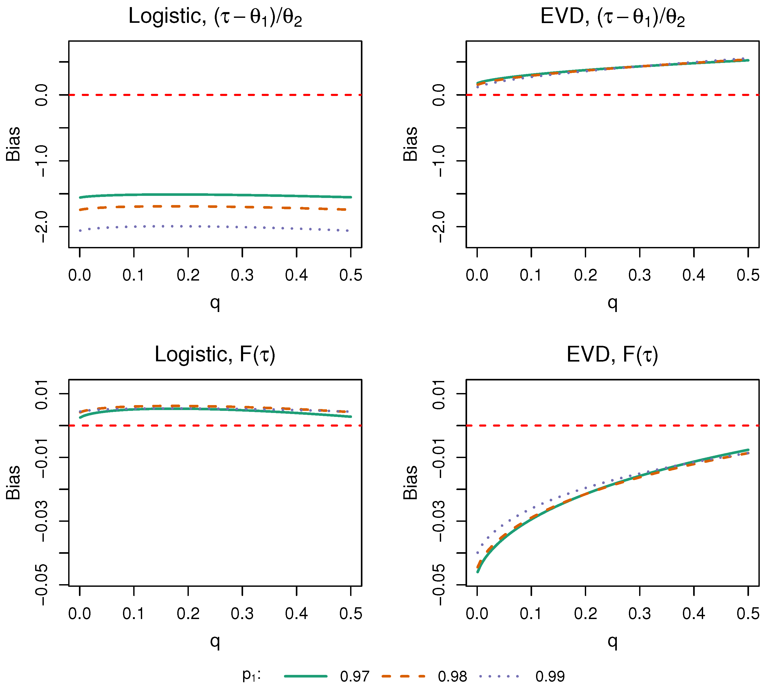
3. Inference Under Model Misspecification

The normal distribution is often the default model for responses in applications, so we next consider properties of estimators and inference procedures when one assumes $Y_1,\dots ,Y_n$ are (independently) generated from a normal distribution with mean ${\theta }_{1a}$ and variance ${\theta }_{2a}^2$ and the data-generating distribution may differ. As illustrations, we consider the cases where Y is generated from (i) a logistic distribution with c.d.f.

$$F_T(y;\theta )={\left\{1+exp\left(-{\displaystyle \frac{y-{\theta }_1}{{\theta }_2}}\right)\right\}}^{-1},$$

(2)

and (ii) an extreme value distribution with c.d.f.

$$F_T(y;\theta )=1-exp\left\{-exp\left({\displaystyle \frac{y-{\theta }_1}{{\theta }_2}}\right)\right\}.$$

(3)

Here, we use subscript T to emphasize that $F_T$ is the true (not assumed) c.d.f. of Y.

Now let $X_i=max(Y_i,d)$ with ${\Delta }_i=I(X_i=Y_i)$, and fix the left-censoring rate $q=P(Y_i\le d)=\mathrm{E}\{1-{\Delta }_i\}$. Then, the observed data likelihood for the assumed normal model is

$$\mathcal{L}({\theta }_a;x,\delta )=\prod _{i=1}^n\left\{{\left[{\displaystyle \frac{1}{{\theta }_{2a}}}exp\left(-{\displaystyle \frac{1}{2}}{\left({\displaystyle \frac{x_i-{\theta }_{1a}}{{\theta }_{2a}}}\right)}^2\right)\right]}^{{\delta }_i}{F}_{a,0}{\left({\displaystyle \frac{x_i-{\theta }_{1a}}{{\theta }_{2a}}}\right)}^{1-{\delta }_i}\right\},$$

or, equivalently,

$$\mathcal{L}({\psi }_a;x,\delta )=\prod _{i=1}^n\left\{{\left[{\psi }_{2a}exp\left(-{\displaystyle \frac{1}{2}}{({\psi }_{1a}+{\psi }_{2a}{x}_i)}^2\right)\right]}^{{\delta }_i}{F}_{a,0}{({\psi }_{1a}+{\psi }_{2a}{x}_i)}^{1-{\delta }_i}\right\}$$

where $F_{a,0}$ denotes the c.d.f. of $N(0,1)$, and ${\psi }_a={({\psi }_{1a},{\psi }_{2a})}^{\prime }={(-{\theta }_{1a}/{\theta }_{2a},1/{\theta }_{2a})}^{\prime }$ such that

$${\psi }_{1a}+{\psi }_{2a}x={\displaystyle \frac{x-{\theta }_{1a}}{{\theta }_{2a}}}.$$

Since ${\delta }_i=I(x_i=y_i)$, we can also write this as

$$\mathcal{L}({\psi }_a;y,\delta )=\prod _{i=1}^n\left\{{\left[{\psi }_{2a}exp\left(-{\displaystyle \frac{1}{2}}{({\psi }_{1a}+{\psi }_{2a}{y}_i)}^2\right)\right]}^{{\delta }_i}{F}_{a,0}{({\psi }_{1a}+{\psi }_{2a}d)}^{1-{\delta }_i}\right\}.$$

(4)

As shown by White [21], the estimator ${\widehat{\psi }}_a$ solves the score equations $S({\psi }_a;y,\delta )={\sum }_{i=1}^n{S}_i({\psi }_a;y_i,{\delta }_i)=0$ corresponding to (4) and satisfies

$$\sqrt{n}({\widehat{\psi }}_a-{\psi }_a^{*})\sim MVN(\mathbf{0},{\mathcal{A}}^{-1}\left({\psi }_a^{*}\right)\mathcal{B}\left({\psi }_a^{*}\right){\mathcal{A}}^{-1}\left({\psi }_a^{*}\right))$$

where

• ${\psi }_a^{*}$ solves ${\mathrm{E}}_T\left\{S_i({\psi }_a;Y_i,{\Delta }_i)\right\}=\int S_i({\psi }_a;y_i,{\delta }_i)d{F}_T(y_i;\psi )=0,$
• $\mathcal{A}\left({\psi }_a^{*}\right)={\mathrm{E}}_T\left\{-{\displaystyle \frac{\partial }{\partial {\psi }_a^{\prime }}}{S}_i({\psi }_a;Y_i,{\Delta }_i)\right\}{|}_{{\psi }_a={\psi }_a^{*}},$ and
• $\mathcal{B}\left({\psi }_a^{*}\right)={\mathrm{E}}_T\left\{S_i({\psi }_a;Y_i,{\Delta }_i)S_i^{\prime }({\psi }_a;Y_i,{\Delta }_i)\right\}{|}_{{\psi }_a={\psi }_a^{*}}$

and ${\mathrm{E}}_T\left\{·\right\}$ denotes the expectation under the true data-generating model; see also Gourieroux, Monfort, and Trognon [22] and Qin and Lawless [23]. Appendix A shows how to compute the limiting values and implicit estimands ${\psi }_a^{*}$ when the true distribution is logistic or extreme value (case (i) or (ii) above, respectively). Recall that ${\psi }_1=-{\theta }_1/{\theta }_2$ and ${\psi }_2=1/{\theta }_2$, so to recover the limiting values of estimates for ${\theta }_1$, $log\left({\theta }_2\right)$, ${\psi }_1+{\psi }_2\tau$, and $F_T(\tau ;\psi )$, we, respectively, use the following:

• $-{\psi }_{1a}^{*}/{\psi }_{2a}^{*}$;
• $-log\left({\psi }_{2a}^{*}\right)$;
• ${\psi }_{1a}^{*}+{\psi }_{2a}^{*}\tau$;
• $F_{a,0}({\psi }_{1a}^{*}+{\psi }_{2a}^{*}\tau )$.

The bias of an estimator is defined as its estimand based on the assumed model minus its intended estimand (e.g., $\mathrm{bias}\left({\widehat{\theta }}_{1a}\right)=-{\psi }_{1a}^{*}/{\psi }_{2a}^{*}-{\theta }_1$). Plots of bias as a function of the left-censoring rate q for the first two estimands listed above are displayed in Figure 1; here, we use scale ${\theta }_2=1$ (i.e., $log\left({\theta }_2\right)=0$), and location ${\theta }_1$, chosen to align the 95th percentile of the data-generating distribution with that of the standard normal, resulting in ${\theta }_1=-1.30$ for the logistic distribution and ${\theta }_1=0.55$ for the extreme value distribution. Examining these plots at $q=0$ shows that, in the absence of an LLD, model misspecification may lead to substantial bias. Note that larger LLDs may or may not be associated with less absolute bias, indicating that a loss of information in the lower tail of the distribution may, in some cases, improve performance in terms of bias but the LLD cannot be relied upon for this purpose.

The bias curves for the second two estimands, displayed in Figure 2, further demonstrate the meaningful bias that may result from model misspecification in the absence of an LLD, even at high reliability levels. As before, increasing the left-censoring rate may or may not reduce bias here, although the reliability estimator under the extreme value error distribution shows marked reduction in asymptotic bias with a larger LLD.

In order to investigate the relationship between the LLD and rejection rates for tests of the hypotheses in Section 2, we next examine the asymptotic rejection rate as a function of the left-censoring rate. We begin by reformulating our hypothesis test in terms of the quantity

$$c^{\prime }\psi ={\displaystyle \frac{\tau -{\theta }_1}{{\theta }_2}}$$

where $c={(1,\tau )}^{\prime }$ and $\psi ={({\psi }_1,{\psi }_2)}^{\prime }={(-{\theta }_1/{\theta }_2,1/{\theta }_2)}^{\prime }$; in particular, since $F_a(\tau ;\psi )=F_{a,0}\left(c^{\prime }\psi \right)$, where $F_{a,0}$ is again the standardized c.d.f. under the assumed model, and we wish to test

$$H_0:F_a(\tau ;\psi )=p_0\mathrm{vs}.H_A:F_a(\tau ;\psi )>p_0,$$

we apply $F_{a,0}^{-1}$ to both sides of each hypothesis to get

$$H_0:c^{\prime }\psi =F_{a,0}^{-1}\left(p_0\right)\mathrm{vs}.H_A:c^{\prime }\psi >F_{a,0}^{-1}\left(p_0\right).$$

Now, let ${\widehat{\psi }}_a$ be the estimate of $\psi$ under the assumed model with limiting value ${\psi }_a^{*}$. Given the robust (“true”) variance ${\mathrm{Var}}_T\left({\widehat{\psi }}_a\right)$ of White [21] and the corresponding variance ${\mathrm{Var}}_a\left({\widehat{\psi }}_a\right)$ under the assumed model, we can compute the asymptotic rejection rate (at the 0.025 one-sided significance level) for our reformulated hypothesis test using

$$P\left({\displaystyle \frac{c^{\prime }{\widehat{\psi }}_a-F_{a,0}^{-1}\left(p_0\right)}{\sqrt{{\mathrm{Var}}_a\left(c^{\prime }{\widehat{\psi }}_a\right)}}}>1.96\right)=1-P\left({\displaystyle \frac{F_{a,0}^{-1}\left(p_0\right)-c^{\prime }{\psi }_a^{*}+1.96\sqrt{c^{\prime }{\mathrm{Var}}_a\left({\widehat{\psi }}_a\right)c}}{\sqrt{c^{\prime }{\mathrm{Var}}_T\left({\widehat{\psi }}_a\right)c}}}\right).$$

(5)

Explicit expressions for ${\mathrm{Var}}_T\left({\widehat{\psi }}_a\right)$ and ${\mathrm{Var}}_a\left({\widehat{\psi }}_a\right)$ are derived under an assumed normal model in Appendix B and Appendix C.

In a statistical hypothesis test, the “type I error rate” refers to the probability of rejecting $H_0$ when it is true (i.e., incorrectly concluding that $p_1>p_0$ when the truth is $p_1=p_0$ in this case), while “power” refers to the probability of rejecting $H_0$ when it is false (i.e., correctly concluding that $p_1>p_0$) across multiple samples from the same population. An illustration of the rejection rates resulting from (5) is shown in Figure 3 (type I error; $p_1=0.95$) and Figure 4 (power; $p_1=0.97,0.98,0.99$), respectively; here, we use $p_0=0.95$, $n=80$, scale ${\theta }_2=1$, and location ${\theta }_1$, chosen to align the $p_1$ quantile of the data-generating distribution with that of the standard normal.

As expected, when the error distribution is normal (and thus matches the assumed model), the type I error rate is at the nominal level of 0.025 (red dashed line in Figure 3) and power is a strictly decreasing function of the left-censoring rate q (Figure 4). When the error distribution is logistic, we see an elevated false positive rate relative to the normal data case (Figure 3) as well as increased power (Figure 4); by contrast, when it is extreme value, the false positive rate is very low and power is also greatly diminished. Inference is invalid in both of these cases due to poor control of the type I error rate. Interestingly, the impact of q on asymptotic power does not depend much on the true reliability level $p_1$ in the normal and logistic error settings but increases substantially as a function of $p_1$ with extreme value errors (Figure 4).

4. A Piecewise-Constant Hazard-Based Model

In Appendix D, we investigate the performance of the Shapiro–Francia test [24] of normality under an LLD and find that some location-scale distributions that differ greatly in their tails (and, therefore, differ greatly in their reliability estimates) may be indistinguishable to whole-distribution goodness of fit tests. Based on this finding, we now introduce a flexible class of models based on piecewise-constant hazard models from the field of survival analysis [18]. This approach requires fewer parametric assumptions and intentionally discards observations in the lower tail of the measurement distribution to improve the robustness of inference in the upper tail.

We first consider non-negative values $V_i=exp\left(Y_i\right)$, $i=1,\dots ,n$, and corresponding threshold value ${\tau }_V=exp\left(\tau \right)$. To limit the influence of observations in the lower tail on inference in the upper tail, we next restrict attention to values of $v>{\tau }_V-ϵ$ for some tolerance $ϵ\ge 0$. In particular, we take $v_0={\tau }_V-ϵ$ and simply assign a mass to the event $V<v_0$ given by $p=P(V<v_0)$. Letting $\eta =\mathrm{logit}\left(p\right)$ yields

$$F_V(v_0;\eta )=P(V<v_0;\eta )={\displaystyle \frac{exp\left(\eta \right)}{1+exp\left(\eta \right)}}=\mathrm{expit}\left(\eta \right).$$

Then, to model ${\mathcal{F}}_V\left(v\right)=1-F_V\left(v\right)$ for $v>v_0$, we partition $(v_0,\infty )$ into K intervals using cut-points $v_0=b_0<b_1<\cdots <b_K=\infty$ and let ${\mathcal{B}}_k=[b_{k-1},b_k)$ for $k=1,\dots ,K$. We then use the model

$${\mathcal{F}}_V(v;p,\rho )=P(V>v;p,\rho )=(1-p)e^{-\Lambda (v_0,v;\rho )}$$

where the following apply:

• $\Lambda (v_0,v;\rho )={\sum }_{k=1}^K{W}_k(v_0,v){\rho }_k$ is the “cumulative hazard”;
• $W_k(v_0,v)={\int }_{v_0}^{v}I(u\in {\mathcal{B}}_k)du$ is the “time at risk” in ${\mathcal{B}}_k$ over the interval $[v_0,v)$.

Letting ${\beta }_k=log{\rho }_k$ for $k=1,\dots ,K$ and $\beta ={({\beta }_1,\dots ,{\beta }_K)}^{\prime }$, we can write

$${\mathcal{F}}_V(v;\eta ,\beta )=(1-\mathrm{expit}\left(\eta \right))exp\left\{-\sum _{k=1}^K{W}_k(v_0,v)e^{{\beta }_k}\right\}.$$

4.1. Maximum Likelihood Estimation

In what follows, we suppress the subscript V on density $f_V$, c.d.f. $F_V$, and survivor function ${\mathcal{F}}_V$ of V, for ease of notation. Since $d{W}_k(v_0,v)/dy=I(v\in {\mathcal{B}}_k)$, then the corresponding density (assuming $v\ge v_0$ so that $I(v\in {\mathcal{B}}_k)=1$ for some $k\in \{1,\dots ,K\}$) is given by

$$f(v;\eta ,\beta )=(1-\mathrm{expit}\left(\eta \right))exp\left\{-\sum _{k=1}^K{W}_k(v_0,v)e^{{\beta }_k}\right\}\sum _{k=1}^{K}I(v\in {\mathcal{B}}_k)e^{{\beta }_k}.$$

(6)

Now, for a sample of n observations from independent units, let ${\delta }_i=I(v_i\ge v_0)$ with ${\delta }_{·}={\sum }_{i=1}^n{\delta }_i$ for $i=1,\dots ,n$. Further, let $S_{ik}=W_k(v_0,v_i)$ with $S_{·k}={\sum }_{i=1}^n{S}_{ik}$ and ${\delta }_{ik}=I(v_i\in {\mathcal{B}}_k)$ with ${\delta }_{·k}={\sum }_{i=1}^n{\delta }_{ik}$ for $k=1,\dots ,K$. Note that since v can only fall in interval ${\mathcal{B}}_k$ if $v\ge v_0$, then ${\delta }_i{\delta }_{ik}={\delta }_{ik}$, and since $S_{ik}=0$ when ${\delta }_i=0$, then ${\delta }_i{S}_{ik}=S_{ik}$. Lastly, we replace ${\sum }_{k=1}^{K}I(v\in {\mathcal{B}}_k)e^{{\beta }_k}$ with ${\prod }_{k=1}^K{e}^{I(v\in {\mathcal{B}}_k){\beta }_k}$ in (6). Then, accounting for both $v\in (0,v_0)$ and $v\in (v_0,\infty )$, the likelihood is

$$\begin{array}{cc}\hfill \mathcal{L}(\eta ,\beta ;v)& =\prod _{i=1}^{n}F{(v_0;\eta )}^{1-{\delta }_i}f{(v_i;\eta ,\beta )}^{{\delta }_i}\hfill \\ \hfill & =\prod _{i=1}^n\left\{{\left[\mathrm{expit}\left(\eta \right)\right]}^{1-{\delta }_i}{\left[(1-\mathrm{expit}\left(\eta \right))exp\left\{-\sum _{k=1}^K{W}_k(v_0,v_i)e^{{\beta }_k}\right\}\prod _{k=1}^K{e}^{I(v_i\in {\mathcal{B}}_k){\beta }_k}\right]}^{{\delta }_i}\right\}\hfill \\ \hfill & ={\left[\mathrm{expit}\left(\eta \right)\right]}^{n-{\delta }_{·}}{(1-\mathrm{expit}\left(\eta \right))}^{{\delta }_{·}}exp\left\{-\sum _{i=1}^n\sum _{k=1}^K{\delta }_i{S}_{ik}{e}^{{\beta }_k}\right\}\left(\prod _{i=1}^n\prod _{k=1}^K{e}^{{\delta }_i{\delta }_{ik}{\beta }_k}\right)\hfill \\ \hfill & ={\left[\mathrm{expit}\left(\eta \right)\right]}^n{\left({\displaystyle \frac{1-\mathrm{expit}\left(\eta \right)}{\mathrm{expit}\left(\eta \right)}}\right)}^{{\delta }_{·}}exp\left\{\sum _{k=1}^K\left({\beta }_k{\delta }_{·k}-S_{·k}{e}^{{\beta }_k}\right)\right\}.\hfill \end{array}$$

(7)

Now, let $\theta ={(\eta ,{\beta }^{\prime })}^{\prime }$. We have

$$\ell \left(\theta \right)=log\mathcal{L}\left(\theta \right)=nlog\left(\mathrm{expit}\left(\eta \right)\right)-\eta {\delta }_{·}+\sum _{k=1}^K\left({\beta }_k{\delta }_{·k}-S_{·k}{e}^{{\beta }_k}\right).$$

Taking the first partial derivatives of $\ell \left(\theta \right)$ and solving the resulting estimating equations readily yields maximum likelihood estimates of

$$\widehat{\eta }=\mathrm{logit}\left(1-{\displaystyle \frac{{\delta }_{·}}{n}}\right)\mathrm{and}{\widehat{\beta }}_k=log\left({\displaystyle \frac{{\delta }_{·k}}{S_{·k}}}\right),k=1,\dots ,K.$$

4.2. Profile Likelihood Ratio Test

To test process reliability using this model, we use a profile likelihood ratio test [16], which is conducted as follows:

• Write $\mathcal{L}(\gamma ,\beta )$ where $\gamma =\gamma \left(\theta \right)=\mathcal{F}({\tau }_V;\theta )$: letting

  $${\mathcal{F}}_1(\tau ;\beta )=exp\left\{-\sum _{k=1}^K{W}_k(v_0,\tau )e^{{\beta }_k}\right\},$$

  we have $\gamma =(1-\mathrm{expit}\left(\eta \right)){\mathcal{F}}_1({\tau }_V;\beta )$, so

  $$\mathrm{expit}\left(\eta \right)={\displaystyle \frac{{\mathcal{F}}_1({\tau }_V;\beta )-\gamma }{{\mathcal{F}}_1({\tau }_V;\beta )}}\mathrm{and}{\displaystyle \frac{1-\mathrm{expit}\left(\eta \right)}{\mathrm{expit}\left(\eta \right)}}={\displaystyle \frac{\gamma }{{\mathcal{F}}_1({\tau }_V;\beta )-\gamma }}.$$

  Hence, continuing from the likelihood function (7) above, we have

  $$\mathcal{L}(\gamma ,\beta )={\gamma }^{{\delta }_{·}}{[{\mathcal{F}}_1({\tau }_V;\beta )-\gamma ]}^{n-{\delta }_{·}}{\mathcal{F}}_1{({\tau }_V;\beta )}^{-n}exp\left\{\sum _{k=1}^K\left({\beta }_k{\delta }_{·k}-S_{·k}{e}^{{\beta }_k}\right)\right\}.$$
• Compute the profile likelihood estimate $\widehat{\beta }\left(\gamma \right)$: We can optimize the log-likelihood

  $$\begin{array}{cc}\hfill \ell (\gamma ,\beta )& ={\delta }_{·}log\gamma +(n-{\delta }_{·})log({\mathcal{F}}_1({\tau }_V;\beta )-\gamma )\hfill \\ \hfill & -nlog{\mathcal{F}}_1({\tau }_V;\beta )+\sum _{k=1}^K\left({\beta }_k{\delta }_{·k}-S_{·k}{e}^{{\beta }_k}\right)\hfill \\ \hfill & ={\delta }_{·}log\gamma +(n-{\delta }_{·})log\left(exp\left\{-\sum _{k=1}^K{W}_k(v_0,{\tau }_V)e^{{\beta }_k}\right\}-\gamma \right)\hfill \\ \hfill & +n\sum _{k=1}^K{W}_k(v_0,{\tau }_V)e^{{\beta }_k}+\sum _{k=1}^K\left({\beta }_k{\delta }_{·k}-S_{·k}{e}^{{\beta }_k}\right).\hfill \end{array}$$

  numerically for a given value of $\gamma$ to get $\widehat{\beta }\left(\gamma \right)$.
• Under $H_0:\gamma ={\gamma }_0$, we have

  $$-2\left[\ell ({\gamma }_0,\widehat{\beta }\left({\gamma }_0\right))-\ell (\tilde{\gamma },\tilde{\beta })\right]\sim {\chi }_{\left(1\right)}^2,$$

  where $\tilde{\eta }$ and $\tilde{\beta }$ are the (non-profile) MLEs derived in Section 4.1, and $\tilde{\gamma }=\tilde{\gamma }(\tilde{\eta },\tilde{\beta })$. Thus, a $100(1-\alpha )\%$ profile likelihood interval for $\gamma$ is given by

  $$\ell (\gamma ,\widehat{\beta }\left(\gamma \right))-\ell (\tilde{\gamma },\tilde{\beta })\ge -{\chi }_{(1,1-\alpha )}^2/2$$

  where ${\chi }_{(1,1-\alpha )}^2$ is the $1-\alpha$ quantile of ${\chi }_{\left(1\right)}^2$.
• Reject $H_0$ if ${\gamma }_0=1-p_0$ falls outside the profile likelihood interval computed in step (3). This constitutes a hypothesis test at significance level $\alpha$.

5. Empirical Studies

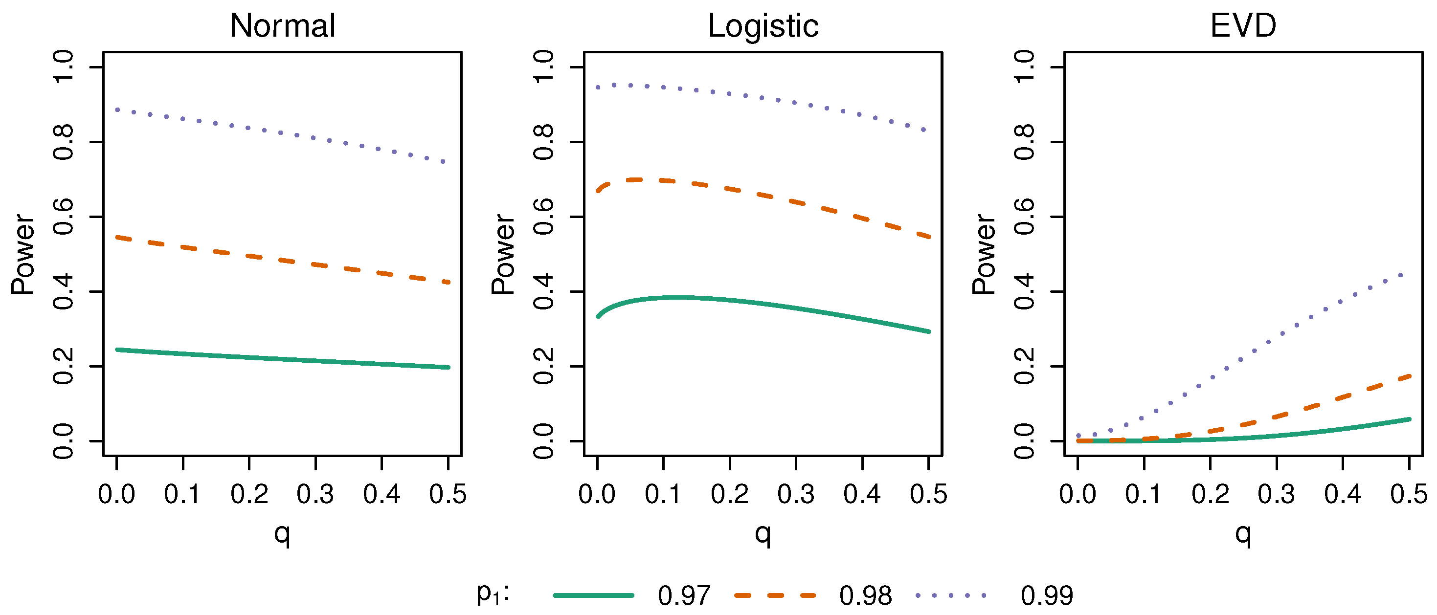
5.1. Bias, Power, Robustness, and Efficiency

To assess the bias and efficiency of estimation and the power of reliability tests for these methods, and to assess their robustness to model misspecification, we consider several simulation studies. In each of the simulations detailed below, two thousand simulation iterations are run and we conduct one-sided tests for $p_0=0.95$ reliability at both the 0.025 and 0.05 significance levels.

For each of the methods, we run a simulation for each combination of (a) sample size n; (b) true reliability $p_1$; (c) true data-generating distribution; (d) fitted model; and (e) LLD value d. Possible sample sizes n include 20, 40, 60, and 80, while possible values for $p_1$ include 0.95 (representing the null hypothesis), 0.97, and 0.99. All true data-generating distributions are set to have scale parameter ${\theta }_2=1$; under this constraint, the possible true distributions include the standard normal, as well as logistic and extreme value distributions, with location parameter ${\theta }_1$ chosen to align the $p_1$ quantile of the true distribution with that of the standard normal. See Equations (2) and (3) for the specification of the logistic and extreme value distributions. Possible fitted models vary depending on the modelling method. In the case of the fully parametric models of Section 2, we fit normal models, so the fitted model is correctly specified when the true data-generating distribution is standard normal but misspecified otherwise. In the case of the piecewise-constant hazard-based models, we let $Q_p$ denote the pth percentile of the true data-generating distribution and consider models with interval cut-points at $b_0=Q_{90}$; $b_0=Q_{85}$, $b_1=Q_{90}$, and $b_2=Q_{95}$; and $b_0=Q_{85}$, $b_1=Q_{89}$, and $b_2=Q_{93}$; as well as models with cut-points at the corresponding empirical percentiles. We focus here on cut-points $Q_p$ with $p\ge 85$ to ensure robustness in approximating the upper tail of the measurement distribution near the critical reliability threshold $\tau$. Varying the LLD only affects the fully parametric method since the other models deliberately avoid distinguishing between observations above and below the LLD for sufficiently small values in $y_1,\dots ,y_n$. For this method, one possible value of the LLD is $d=Q_{10}^N$ where $Q_p^N$ denotes the pth percentile of the standard normal distribution. Under this LLD, the asymptotic percentage of left-censored observations is 10% when fitting a normal model but greater than 10% when fitting logistic or extreme value models. Thus, to disentangle the effects of these differing left-censoring rates from the effects of model misspecification itself, we also consider an LLD of $d=Q_{10}$, based on the true data-generating distribution.

In order to more extensively explore the spectrum of models from fully parametric to fully non-parametric, we compare the results of the normal and piecewise-constant hazard-based models to those obtained using a non-parametric method, where p-values and smoothed “mid-p” values are computed according to a one-sided exact binomial test [25].

A selection of simulation results is shown in

Table 1. Estimates of $F\left(\tau \right)$ obtained under 10% left-censoring based on 2000 simulated samples of size n.

$\mathit{F}\left(\mathit{\tau }\right)$	Data-Generating Model	n	Normal	Piecewise-Constant 1			Exact Test
				${\widehat{Q}}_{90}$	${\widehat{Q}}_{85,90,95}$	${\widehat{Q}}_{85,89,93}$
0.95	Normal	20	0.949	0.957	0.955		0.949
		40	0.950	0.951	0.951	0.950	0.949
		60	0.950	0.949	0.950	0.946	0.949
		80	0.949	0.947	0.950	0.947	0.949
	Logistic	20	0.951	0.953	0.955		0.950
		40	0.950	0.943	0.949	0.945	0.949
		60	0.951	0.938	0.948	0.940	0.950
		80	0.951	0.935	0.947	0.941	0.950
	Extreme Value	20	0.925	0.959	0.957		0.951
		40	0.923	0.954	0.952	0.952	0.950
		60	0.923	0.952	0.951	0.948	0.949
		80	0.923	0.952	0.951	0.949	0.949
0.97	Normal	20	0.968	0.972	0.972		0.969
		40	0.969	0.970	0.970	0.970	0.969
		60	0.969	0.969	0.969	0.968	0.969
		80	0.969	0.968	0.969	0.968	0.969
	Logistic	20	0.973	0.969	0.973		0.970
		40	0.973	0.962	0.968	0.966	0.969
		60	0.974	0.958	0.966	0.961	0.969
		80	0.974	0.956	0.965	0.960	0.970
	Extreme Value	20	0.942	0.974	0.974		0.970
		40	0.941	0.972	0.971	0.972	0.969
		60	0.941	0.971	0.970	0.971	0.969
		80	0.941	0.971	0.970	0.971	0.969
0.99	Normal	20	0.988	0.990	0.990		0.990
		40	0.989	0.990	0.989	0.990	0.990
		60	0.989	0.990	0.989	0.991	0.990
		80	0.989	0.990	0.989	0.990	0.989
	Logistic	20	0.993	0.989	0.991		0.990
		40	0.994	0.987	0.989	0.988	0.990
		60	0.994	0.986	0.988	0.987	0.990
		80	0.995	0.986	0.987	0.986	0.990
	Extreme Value	20	0.964	0.989	0.990		0.991
		40	0.964	0.989	0.990	0.990	0.990
		60	0.964	0.989	0.990	0.991	0.990
		80	0.964	0.990	0.990	0.990	0.990

¹ Column heading indicates the $p_1,\dots ,p_K$ empirical percentiles ${\widehat{Q}}_{p_1,\dots ,p_K}$ defining the interval cut-points of the fitted piecewise-constant hazard-based model.

and

Table 2. Empirical null hypothesis rejection rates at the $\alpha =0.025$ significance level, testing for 95% reliability under 10% left-censoring, based on 2000 simulated samples of size n.

$\mathit{F}\left(\mathit{\tau }\right)$	Data-Generating Model	n	Normal	Piecewise-Constant 1			Exact Test
				${\widehat{Q}}_{90}$	${\widehat{Q}}_{85,90,95}$	${\widehat{Q}}_{85,89,93}$	p-Value	mid-p
0.95	Normal	20	0.039	0.035	0.015		0.000	0.000
		40	0.029	0.031	0.042	0.048	0.000	0.000
		60	0.031	0.026	0.035	0.053	0.000	0.045
		80	0.026	0.023	0.032	0.037	0.020	0.020
	Logistic	20	0.048	0.059	0.017		0.000	0.000
		40	0.049	0.047	0.044	0.056	0.000	0.000
		60	0.050	0.042	0.042	0.058	0.000	0.050
		80	0.058	0.028	0.030	0.033	0.021	0.021
	Extreme Value	20	0.002	0.027	0.018		0.000	0.000
		40	0.000	0.022	0.030	0.039	0.000	0.000
		60	0.001	0.023	0.029	0.044	0.000	0.048
		80	0.000	0.019	0.029	0.034	0.017	0.017
0.97	Normal	20	0.100	0.072	0.032		0.000	0.000
		40	0.124	0.087	0.077	0.090	0.000	0.000
		60	0.177	0.113	0.085	0.137	0.000	0.153
		80	0.225	0.125	0.111	0.128	0.090	0.090
	Logistic	20	0.167	0.132	0.037		0.000	0.000
		40	0.241	0.169	0.110	0.159	0.000	0.000
		60	0.340	0.155	0.119	0.166	0.000	0.164
		80	0.405	0.154	0.120	0.144	0.093	0.093
	Extreme Value	20	0.005	0.059	0.023		0.000	0.000
		40	0.003	0.064	0.062	0.080	0.000	0.000
		60	0.002	0.089	0.076	0.129	0.000	0.156
		80	0.000	0.108	0.098	0.116	0.078	0.078
0.99	Normal	20	0.355	0.192	0.055		0.000	0.000
		40	0.639	0.374	0.253	0.364	0.000	0.000
		60	0.848	0.524	0.406	0.557	0.000	0.538
		80	0.924	0.620	0.524	0.604	0.429	0.429
	Logistic	20	0.583	0.339	0.112		0.000	0.000
		40	0.846	0.539	0.383	0.486	0.000	0.000
		60	0.958	0.603	0.474	0.580	0.000	0.538
		80	0.989	0.648	0.541	0.608	0.448	0.448
	Extreme Value	20	0.029	0.132	0.044		0.000	0.000
		40	0.035	0.273	0.200	0.277	0.000	0.000
		60	0.048	0.435	0.364	0.515	0.000	0.557
		80	0.072	0.590	0.542	0.603	0.459	0.459

¹ Column heading indicates the $p_1,\dots ,p_K$ empirical percentiles ${\widehat{Q}}_{p_1,\dots ,p_K}$ defining the interval cut-points of the fitted piecewise-constant hazard-based model.

(full results can be found in the Supplementary Materials online). Table 1 shows the estimates of $F\left(\tau \right)$ obtained using each of the models described above, while Table 2 shows the corresponding rejection rates for testing $H_0:F\left(\tau \right)=p_0$ vs. $H_A:F\left(\tau \right)>p_0$ where $p_0=0.95$. In each table, the first section of twelve lines shows the results of simulating data under the null hypothesis that reliability is at the nominal level of $p_0=0.95$, while in the second and third sections, the reliability exceeds $p_0$. Note that each column heading for the piecewise-constant hazard-based models indicates the $p_1,\dots ,p_K$ empirical percentiles ${\widehat{Q}}_{p_1,\dots ,p_K}$ defining the interval cut-points of the fitted model; the model with cut-points at ${\widehat{Q}}_{85}$, ${\widehat{Q}}_{89}$, and ${\widehat{Q}}_{93}$ is omitted when $n=20$ since no observations would fall in the interval $[{\widehat{Q}}_{85},{\widehat{Q}}_{89})$, and such a model would, therefore, not be used in this case.

The leftmost column of Table 1 shows that while fitting a normal model leads to accurate estimates of $F\left(\tau \right)$ when the data are truly normal, bias becomes appreciable under the logistic and, particularly, the extreme value error distribution; this matches the asymptotic results shown in Figure 2. Similarly, Table 2 shows that type I error is well controlled and power reasonably high for larger sample sizes under correct model specification, but (as expected based on Figure 3 and Figure 4) these rejection rates are inflated and severely depressed, respectively, for the logistic and extreme value error distributions. The last column of Table 1 and the last two columns of Table 2 show that the exact tests address the bias issue and perform roughly the same across all settings since they do not rely on distributional assumptions; both p-values and mid-p-values here result in very low rejection rates, however, even when the true reliability of $F\left(\tau \right)=0.99$ far exceeds the nominal reliability of 0.95 that we aim to demonstrate. Prohibitively large sample sizes would be required to achieve acceptable levels of power using exact tests.

The piecewise-constant hazard-based models generally outperform the normal model in terms of both bias in the reliability estimate (Table 1) and power (Table 2) when the data are extreme value, while at the same time, they perform comparably to the normal model when data are generated under a normal or logistic distribution. Bias is least for larger values of $F\left(\tau \right)$ where down-weighted values in the left tail become less relevant for estimation (Table 1). Type I error is relatively well controlled for all simulation settings, particularly at larger sample sizes, which is a notable improvement in the cases of logistic and extreme value data generation (Table 2). Overall, the piecewise-constant hazard-based method provides a balance between the power obtained by correctly specified parametric models and the robustness of non-parametric methods. While the small sample sizes we have focused on here are typical in reliability studies, the performance of these piecewise-constant models is highly scalable as larger samples would allow one to increase the number of cut-points (thereby increasing flexibility and robustness) without sacrificing power.

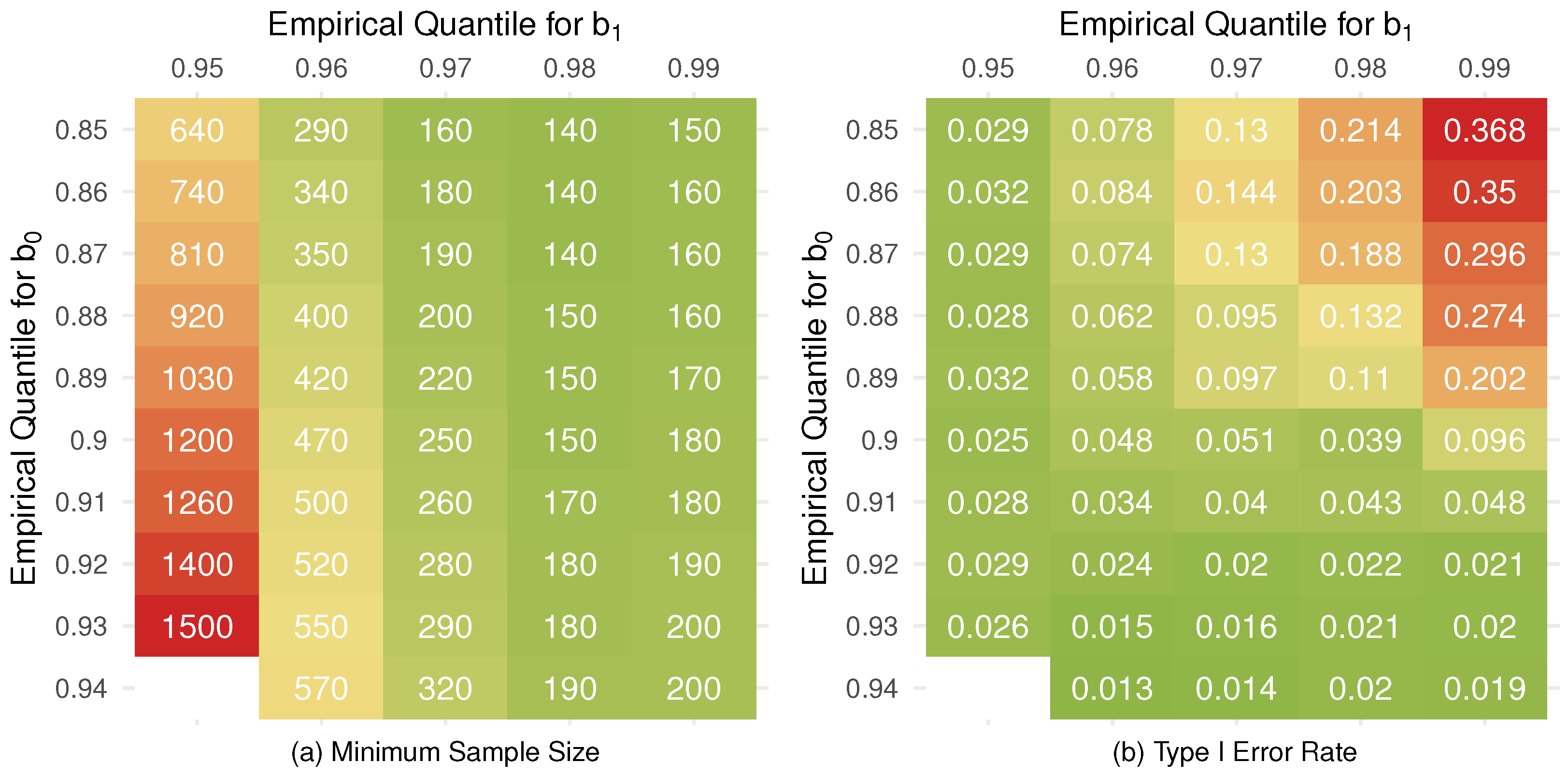
5.2. Model Selection

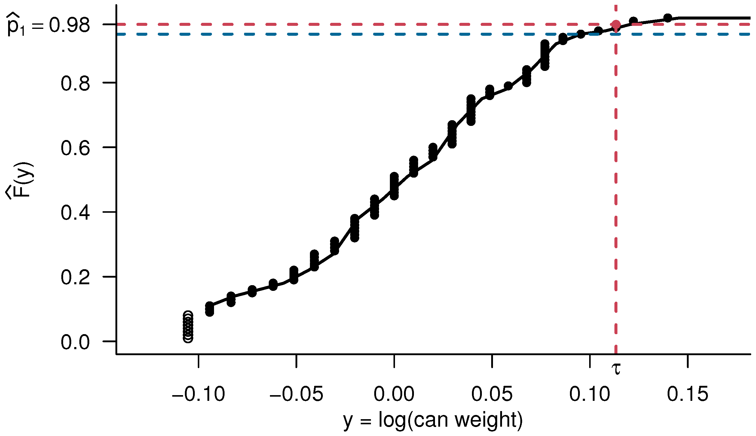
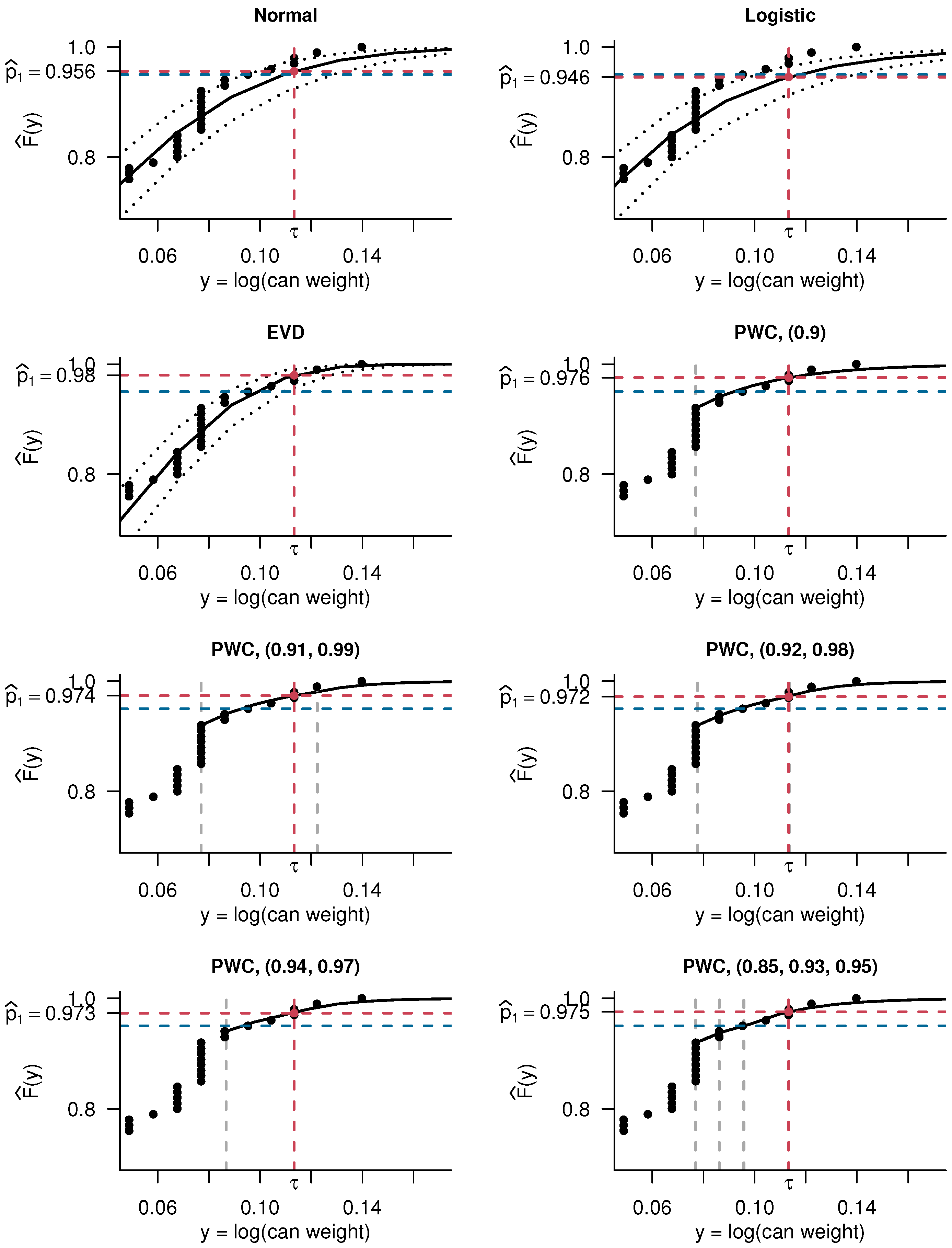
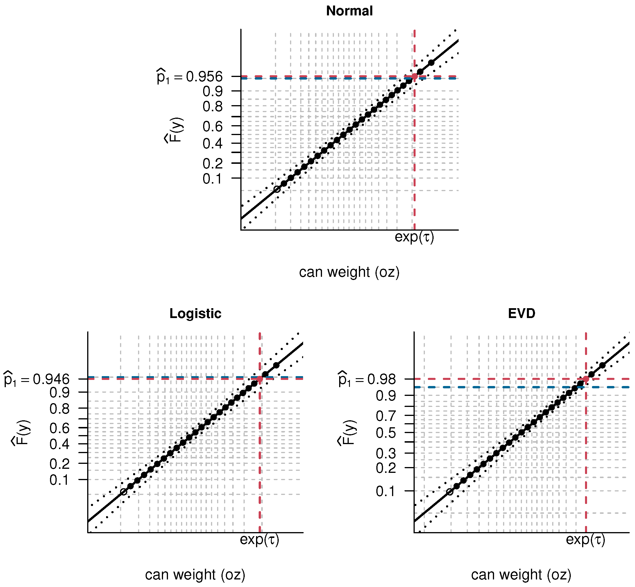
Although Table 1 and Table 2 show that no one piecewise-constant hazard-based model uniformly outperforms the others, model cut-points may be chosen by optimizing the worst possible outcome across all simulation settings. Figure 5 shows the minimum sample size needed to achieve the worst-case empirical power of 90% across normal, logistic, and extreme value data-generating distributions, using a piecewise-constant hazard-based model with two cut-points $b_0$ and $b_1$, as well as the largest possible empirical type I error rate across those distributions when the sample size is fixed at this optimal value. As before, each of these distributions has ${\theta }_2=1$ and a 95th percentile equal to that of a standard normal.

Here, we see that when testing for $p_0=0.95$ and the true reliability is $p_1=0.99$, the two-cut-point model that best balances power and the type I error rate appears to have its cut-points at the 90th and 98th percentiles of the observed data (Figure 5). It is important to note that even in this optimal case, we require a sample size of 150 to achieve the desired power of 90%, and the corresponding type I error rate is slightly inflated at 0.039. If controlling the type I error rate is of greater importance, one may prefer a model with cut-points at the 92nd and 98th percentiles, where we see a required sample size of 180 and a worst-case type I error rate of 0.022.

Figure 5 illustrates the trade-off between type I error rates and the sample sizes required to achieve the specified power level using two-cut-point models (for particular values of $p_0$, $p_1$, threshold $\tau$, significance level $\alpha$, and worst-case empirical power), and similar analyses could be conducted for different choices of tolerance $ϵ$ and number of intervals K (as well as other specifications of the reliability test). Piecewise-constant hazard-based models do not typically require many cut-points to accurately capture the shape of the target distribution [26], and in the context of reliability studies, we recommend using two to four cut-points ($1\le K\le 3$). Moreover, the smaller the tolerance $ϵ$, the closer the first cut-point $b_0$ will be to the exponentiated threshold ${\tau }_V$ and the closer the piecewise-constant hazard-based reliability test will be to the exact binomial test from Section 5.1; smaller $ϵ$ values, therefore, result in greater robustness but worse efficiency, as seen by the larger sample sizes and better-controlled type I error rates at the lower ends of Figure 5a and Figure 5b, respectively. The effects of changing the number and spacing of the other cut-points are more difficult to characterize, and fitting multiple models is recommended in practice to assess the sensitivity of results to a given choice.

6. Application

In this section, we apply the piecewise-constant hazard-based models introduced in Section 4 to a study of drink can weights, used as an example in the documentation for the PROC CAPABILITY statement in SAS^® version 9.4 [27], and we compare the results to those obtained using the fully parametric models of Section 2. The corresponding dataset consists of 100 can weights that we suppose were measured using an industrial scale with an LLD of 0.9 oz; eight of these measurements fall below the LLD, while 98 fall below the threshold $exp\left(\tau \right)=1.12$. Here, interest may lie in demonstrating that at least 95% of cans weigh at most 1.12 oz (say, in order to meet freight shipment weight limits). We therefore aim to test $H_0:F\left(\tau \right)=p_0$ vs. $H_A:F\left(\tau \right)>p_0$ where $\tau =log\left(1.12\right)$, $p_0=0.95$, and F is the c.d.f. of the distribution of log-can weights. We perform analysis on the log scale, as indicated in Section 2.

Figure 6 shows the empirical c.d.f. of the data for observations above the LLD. Non-parametric methods yield $\widehat{F}\left(\tau \right)=98/100=0.98$, with exact binomial tests resulting in

$$p\text{-}\mathrm{value}=\sum _{u=98}^{100}\left({\displaystyle \genfrac{}{}{0pt}{}{100}{u}}\right)·0.{95}^u·{(1-0.95)}^{100-u}=0.118$$

and

$$\mathrm{mid}\text{-}p\text{-}\mathrm{value}=p\text{-}\mathrm{value}-{\displaystyle \frac{1}{2}}\left[\left({\displaystyle \genfrac{}{}{0pt}{}{100}{98}}\right)·0.{95}^{98}·{(1-0.95)}^{100-98}\right]=0.078.$$

While the estimate $\widehat{F}\left(\tau \right)$ is above $p_0=0.95$, neither the p-value nor the mid-p-value provides evidence of process reliability at the 0.025 significance level.

The upper tails of various fitted fully parametric (Section 2) and piecewise-constant hazard-based (Section 4) models are shown in Figure 7, with corresponding reliability estimates and p-values shown in

Table 3. Reliability estimates at threshold $\tau =log\left(1.12\right)$ and corresponding confidence/likelihood intervals obtained for the distribution of log-can weights using fully parametric and piecewise-constant hazard-based models.

Model 1	$\widehat{\mathit{F}}\left(\mathit{\tau }\right)$	Confidence/Likelihood Interval 2
Normal	0.961	$(0.920,0.983)$
Logistic	0.951	$(0.839,0.986)$
Extreme Value	0.982	$(0.965,0.992)$
$\left({\widehat{Q}}_{90}\right)$	0.976	$(0.952,1.000)$
$({\widehat{Q}}_{91},{\widehat{Q}}_{99})$	0.974	$(0.949,1.000)$
$({\widehat{Q}}_{92},{\widehat{Q}}_{98})$	0.972	$(0.922,0.994)$
$({\widehat{Q}}_{94},{\widehat{Q}}_{97})$	0.973	$(0.881,0.993)$
$({\widehat{Q}}_{85},{\widehat{Q}}_{93},{\widehat{Q}}_{95})$	0.975	$(0.929,1.000)$

¹ Each piecewise-constant hazard-based model (last five rows) is specified by the vector of empirical pth percentiles ${\widehat{Q}}_p$ used as its cut-points. ² This is a two-sided 95% confidence interval for the fully parametric models (first three rows) and a one-sided 97.5% likelihood interval for the piecewise-constant hazard-based models (last five rows).

. Here, we fit logistic and extreme value models in addition to the normal models examined in the derivations of Appendix A–Appendix C and the simulation study of Section 5.1. Each piecewise-constant hazard-based model is specified by either the vector of empirical pth percentiles ${\widehat{Q}}_p$ used as its cut-points (Table 3) or, for ease of plotting, the corresponding vector of probabilities p (Figure 7); these models are chosen as follows:

• $\left({\widehat{Q}}_{90}\right)$ is one of the models considered in the simulation study of Section 5.1;
• $({\widehat{Q}}_{85},{\widehat{Q}}_{93},{\widehat{Q}}_{95})$ is an adaptation of another model $({\widehat{Q}}_{85},{\widehat{Q}}_{90},{\widehat{Q}}_{95})$ from the simulation study, with the middle cut-point adjusted upward to ensure that each interval of the resulting model strictly contains at least one observation;
• $({\widehat{Q}}_{92},{\widehat{Q}}_{98})$ is suggested by the simulation from Section 5.2;
• $({\widehat{Q}}_{91},{\widehat{Q}}_{99})$ and $({\widehat{Q}}_{94},{\widehat{Q}}_{97})$ are the models that are, respectively, the closest to and farthest from demonstrating reliability from a grid search of two-cut-point models whose first cut-point is in $\{{\widehat{Q}}_{91},{\widehat{Q}}_{92},{\widehat{Q}}_{93},{\widehat{Q}}_{94}\}$ and whose second cut-point is in $\{{\widehat{Q}}_{95},{\widehat{Q}}_{96},\dots ,{\widehat{Q}}_{99}\}$.

Note that the third model $({\widehat{Q}}_{85},{\widehat{Q}}_{89},{\widehat{Q}}_{93})$ from the simulation study is omitted because ${\widehat{Q}}_{85}={\widehat{Q}}_{89}$ for this dataset, meaning that it is effectively a two-cut-point model.

Table 3 shows that, as with the non-parametric method, each of these eight model-based reliability estimates falls above the desired level of $p_0=0.95$. Unlike the exact binomial test, however, some of the corresponding confidence and likelihood intervals have lower limits above 0.95 and, therefore, suggest that the drink can manufacturing process is reliable. We also see that likelihood intervals based on the piecewise-constant hazard-based models are much less variable than the confidence intervals based on their fully parametric counterparts.

Practitioners often use so-called probability plots to visualize the outcomes of fully parametric model fitting, and these are shown in Figure 8. Here, we plot the log-can weights y on the horizontal axis and ${\widehat{\psi }}_1+{\widehat{\psi }}_{2}y$ on the vertical axis but label these axes with can weights $exp\left(y\right)$ and reliability estimates $F_{a,0}({\widehat{\psi }}_1+{\widehat{\psi }}_{2}y)$, respectively, where $F_{a,0}$ is the c.d.f. of the assumed standard error distribution; see Section 2 for the definition of $\psi$.

7. Conclusions

The impact of an LLD on inference in the centre of a distribution has been well studied in the environmental science literature. In this paper, we show that when interest lies in the right tail of the distribution and parametric models are misspecified, an LLD can attenuate bias and even slightly increase the power of tests for reliability, but these modest benefits are not guaranteed and, critically, come at the cost of invalid inference due to poor control of type I error rates. Moreover, the power of goodness of fit tests can be limited even with larger sample sizes, and the presence of an LLD exacerbates this issue; selection of an appropriate fully parametric model, therefore, presents a substantial challenge. In order to circumvent this challenge, we introduce a weakly parametric method of testing process reliability based on piecewise-constant hazard models that de-emphasizes observations in the lower tail of the measurement distribution and successfully balances efficiency with robustness to model misspecification. We use simulations to identify two two-cut-point piecewise-constant hazard-based models that may provide good asymptotic results for particular values of the true and required reliability levels, and apply the methods discussed in this paper to a study of drinking can weights.

While the methods proposed here provide a basic framework for right-tail inference under an LLD, one limitation is that (as seen by Figure 5) the results from piecewise-constant hazard-based models are somewhat sensitive to one’s choice of cut-points. To address this issue, one could consider using splines (say, using survPen in R version 4.3.2 [28]), which may offer more robustness at a modest price in terms of efficiency and power. Practical considerations can also complicate analysis. One such issue is that LLDs may vary between subsets of observations; for example, systematic variation might occur if technological advancements decrease an LLD over time by improving measurement device precision [5,9], while random variation might occur if environmental factors such as wind speed or ambient temperature affect device performance [29]. In other settings involving multiple laboratories, different devices may be used to measure concentrations of analytes, so device-to-device variation in detection limits can also raise challenges. Models for the LLD may be helpful in these situations. Other practical issues that merit attention occur when multiple different LLDs are present (e.g., due to use of multiple measurement devices) and when measurements between the LLD and a so-called “limit of quantification” are said by the device manufacturer to be observed with some uncertainty. More work is required to develop methods suited to these more complicated settings.

Finally, one reviewer raised the notion of Bayesian reliability testing. As noted in Section 1, when one uses fully parametric models of the form presented in Section 2, Bayesian methods have been found to estimate the 95th percentile comparably (at best) to substitution methods [17]. A Bayesian approach could also be compatible, however, with the piecewise-constant hazard-based models that we have proposed here. In particular, one would need to specify a prior for each parameter in the model (e.g., a gamma prior for the exponential hazard rate in each piece [30] and a beta prior for the probability p), calculate the posterior distribution for the true reliability $p_1$, and stipulate a decision rule for using this posterior to conduct the test of reliability given by (1). Such a test could be done by constructing a $100(1-\alpha )\%$ credible interval for $p_1$ and checking whether it covers $p_0$ [31]. This is an interesting possible direction for future research.

References

1. United States Food and Drug Administration. Considerations for the Development of Dried Plasma Products Intended for Transfusion: Guidance for Industry; Docket Number FDA-2018-D-3759; United States Food and Drug Administration: Silver Spring, MD, USA, 2019. Available online: https://www.fda.gov/regulatory-information/search-fda-guidance-documents/considerations-development-dried-plasma-products-intended-transfusion (accessed on 17 October 2024).
2. United States Food and Drug Administration. Submission and Review of Sterility Information in Premarket Notification (510(k)) Submissions for Devices Labeled as Sterile: Guidance for Industry and Food and Drug Administration Staff; Docket Number FDA-2008-D-0611; United States Food and Drug Administration: Silver Spring, MD, USA, 2024. Available online: https://www.fda.gov/regulatory-information/search-fda-guidance-documents/submission-and-review-sterility-information-premarket-notification-510k-submissions-devices-labeled (accessed on 17 October 2024).
3. United States Food and Drug Administration. Approaches to Establish Thresholds for Major Food Allergens and for Gluten in Food; United States Food and Drug Administration: Silver Spring, MD, USA, 2006. Available online: https://www.fda.gov/food/food-labeling-nutrition/approaches-establish-thresholds-major-food-allergens-and-gluten-food (accessed on 17 October 2024).
4. Government of Ontario. R.R.O. 1990, Reg. 347: General—Waste Management. In Environmental Protection Act; Government of Ontario: Toronto, ON, Canada, 2024. Available online: https://www.ontario.ca/laws/regulation/900347 (accessed on 17 October 2024).
5. Newman, M.C.; Dixon, P.M.; Looney, B.B.; Pinder, J.E., III. Estimating Mean and Variance for Environmental Samples with Below Detection Limit Observations. JAWRA J. Am. Water Resour. Assoc. 1989, 25, 905–916. [Google Scholar] [CrossRef]
6. Helsel, D.R. Much Ado About Next to Nothing: Incorporating Nondetects in Science. Ann. Occup. Hyg. 2010, 54, 257–262. [Google Scholar] [CrossRef] [PubMed]
7. Hwang, M.; Lee, S.C.; Park, J.-H.; Choi, J.; Lee, H.-J. Statistical methods for handling nondetected results in food chemical monitoring data to improve food risk assessments. Food Sci. Nutr. 2023, 11, 5223–5235. [Google Scholar] [CrossRef] [PubMed]
8. Gilliom, R.J.; Helsel, D.R. Estimation of Distributional Parameters for Censored Trace Level Water Quality Data: 1. Estimation Techniques. Water Resour. Res. 1986, 22, 135–146. [Google Scholar] [CrossRef]
9. Helsel, D.R.; Cohn, T.A. Estimation of Descriptive Statistics for Multiply Censored Water Quality Data. Water Resour. Res. 1988, 24, 1997–2004. [Google Scholar] [CrossRef]
10. Farewell, V.T. Some comments on analysis techniques for censored water quality data. Environ. Monit. Assess. 1989, 13, 285–294. [Google Scholar] [CrossRef]
11. Shumway, R.H.; Azari, R.S.; Kayhanian, M. Statistical Approaches to Estimating Mean Water Quality Concentrations with Detection Limits. Environ. Sci. Technol. 2002, 36, 3345–3353. [Google Scholar] [CrossRef]
12. Antweiler, R.C.; Taylor, H.E. Evaluation of statistical treatments of left-censored environmental data using coincident uncensored data sets: I. Summary statistics. Environ. Sci. Technol. 2008, 42, 3732–3738. [Google Scholar] [CrossRef]
13. Shoari, N.; Dubé, J.-S.; Chenouri, S. On the use of the substitution method in left-censored environmental data. Hum. Ecol. Risk Assess. Int. J. 2015, 22, 435–446. [Google Scholar] [CrossRef]
14. Tekindal, M.A.; Erdoğan, B.D.; Yavuz, Y. Evaluating Left-Censored Data Through Substitution, Parametric, Semi-parametric, and Nonparametric Methods: A Simulation Study. Interdiscip. Sci. Comput. Life Sci. 2017, 9, 153–172. [Google Scholar] [CrossRef]
15. Kaplan, E.L.; Meier, P. Nonparametric Estimation from Incomplete Observations. J. Am. Stat. Assoc. 1958, 53, 457–481. [Google Scholar] [CrossRef]
16. Sprott, D.A. Statistical Inference in Science; Springer: New York, NY, USA, 2000. [Google Scholar] [CrossRef]
17. Huynh, T.; Quick, H.; Ramachandran, G.; Banerjee, S.; Stenzel, M.; Sandler, D.P.; Engel, L.S.; Kwok, R.K.; Blair, A.; Stewart, P.A. A Comparison of the β-Substitution Method and a Bayesian Method for Analyzing Left-Censored Data. Ann. Occup. Hyg. 2016, 60, 56–73. [Google Scholar] [CrossRef]
18. Lawless, J.F. Statistical Models and Methods for Lifetime Data, 2nd ed.; John Wiley & Sons: Hoboken, NJ, USA, 2003. [Google Scholar] [CrossRef]
19. Therneau, T.M.; Grambsch, P.M. Modeling Survival Data: Extending the Cox Model; Springer: New York, NY, USA, 2000. [Google Scholar]
20. Casella, G.; Berger, R.L. Statistical Inference, 2nd ed.; Duxbury: Pacific Grove, CA, USA, 2002. [Google Scholar]
21. White, H. Maximum likelihood estimation of misspecified models. Econometrica 1982, 50, 1–25. [Google Scholar] [CrossRef]
22. Gourieroux, C.; Monfort, A.; Trognon, A. Pseudo Maximum Likelihood Methods: Theory. Econometrica 1984, 52, 681–700. [Google Scholar] [CrossRef]
23. Qin, J.; Lawless, J. Empirical Likelihood and General Estimating Equations. Ann. Stat. 1994, 22, 300–325. [Google Scholar] [CrossRef]
24. Shapiro, S.S.; Francia, R.S. An Approximate Analysis of Variance Test for Normality. J. Am. Stat. Assoc. 1972, 67, 215–216. [Google Scholar] [CrossRef]
25. Berry, G.; Armitage, P. Mid-P confidence intervals: A brief review. J. R. Stat. Soc. Ser. D Stat. 1995, 44, 417–423. [Google Scholar] [CrossRef]
26. Lawless, J.F.; Zhan, M. Analysis of interval-grouped recurrent event data using piecewise-constant rate functions. Can. J. Stat. 1998, 26, 549–565. [Google Scholar] [CrossRef]
27. SAS Institute Inc. Reading Spec Limits from an Input Data Set; SAS Institute Inc.: Cary, NC, USA, n.d.; Available online: https://documentation.sas.com/doc/en/pgmsascdc/9.4_3.4/qcug/qcug_code_capspec2.htm (accessed on 11 January 2025).
28. Fauvernier, M.; Remontet, L.; Uhry, Z.; Bossard, N.; Roche, L. survPen: An R package for hazard and excess hazard modelling with multidimensional penalized splines. J. Open Source Softw. 2019, 4, 1434. [Google Scholar] [CrossRef]
29. Wigle, A.; Béliveau, A.; Blackmore, D.; Lapeyre, P.; Osadetz, K.; Lemieux, C.; Daun, K.J. Estimation and Applications of Uncertainty in Methane Emissions Quantification Technologies: A Bayesian Approach. ACS ES T Air 2024, 1, 1000–1014. [Google Scholar] [CrossRef]
30. Arjas, E.; Gasbarra, D. Nonparametric Bayesian Inference from Right Censored Survival Data, Using the Gibbs Sampler. Stat. Sin. 1994, 4, 505–524. [Google Scholar]
31. Ghosh, J.K.; Delampady, M.; Samanta, T. An Introduction to Bayesian Analysis: Theory and Methods, 1st ed.; Springer: New York, NY, USA, 2006. [Google Scholar]
32. Millard, S.P. EnvStats: An R Package for Environmental Statistics; Springer: New York, NY, USA, 2013. [Google Scholar]
33. Blom, G. Statistical Estimates and Transformed Beta-Variables; John Wiley & Sons: Hoboken, NJ, USA, 1958. [Google Scholar]
34. Weisberg, S.; Bingham, C. An Approximate Analysis of Variance Test for Non-Normality Suitable for Machine Calculation. Technometrics 1975, 17, 133–134. [Google Scholar] [CrossRef]
35. Royston, P. A Toolkit for Testing for Non-Normality in Complete and Censored Samples. J. R. Stat. Soc. Ser. D Stat. 1993, 42, 37–43. [Google Scholar] [CrossRef]
36. Verrill, S.; Johnson, R.A. Tables and Large-Sample Distribution Theory for Censored-Data Correlation Statistics for Testing Normality. J. Am. Stat. Assoc. 1988, 83, 1192–1197. [Google Scholar] [CrossRef]
Figure 1. Asymptotic bias of estimates for location parameter θ 1 and log-scale parameter log ( θ 2 ) as a function of the left-censoring rate q under logistic (left panels) and extreme value (right panels) error distributions. The red dashed line represents the reference value of zero asymptotic bias.
Mathematics 13 01274 g001
Figure 2. Asymptotic bias of estimates for standardized threshold value ( τ θ 1 ) / θ 2 and reliability F ( τ ) as a function of the left-censoring rate q under logistic (left panels) and extreme value (right panels) error distributions. The red dashed line represents the reference value of zero asymptotic bias.
Mathematics 13 01274 g002
Figure 3. Asymptotic type I error rate for a hypothesis test of H 0 : p 1 = 0.95 vs. H A : p 1 > 0.95 as a function of the left-censoring rate q under logistic and extreme value (EVD) data generation. The red dashed lines indicate the nominal type I error rate of α = 0.025 . Sample size is n = 80 .
Mathematics 13 01274 g003
Figure 4. Asymptotic power for hypothesis tests of H 0 : p 1 = 0.95 vs. H A : p 1 > 0.95 as a function of the left-censoring rate q under normal, logistic, and extreme value (EVD) data generation. Sample size is n = 80 .
Mathematics 13 01274 g004
Figure 5. (a) Minimum sample size n needed to achieve worst-case empirical power of 90% across normal, logistic, and extreme value data-generating distributions, using a piecewise-constant hazard-based model with two cut-points b 0 and b 1 at the specified empirical quantiles; and (b) worst-case empirical type I error rate across those distributions when the sample size in each case is the value n shown in (a). Tests are conducted at the 0.025 significance level with p 0 = 0.95 and p 1 = 0.99 , and each empirical rejection rate is obtained using 2000 simulations. Green cells indicate more desirable configurations of sample size and control of type I error while red cells indicate configurations with impractically large sample sizes or unacceptably elevated type I error rates.
Mathematics 13 01274 g005
Figure 6. Empirical c.d.f. of the log-can weight distribution. Open and closed circles, respectively, denote observations below and above the LLD. The dashed blue line shows the target reliability level of p 0 = 0.95 , while the dashed red lines show the non-parametric reliability estimate p ^ 1 .
Mathematics 13 01274 g006
Figure 7. Fitted c.d.f.s of the log-can weight distribution based on fully parametric and piecewise-constant hazard-based models. Dotted black lines show 95% CIs for the fully parametric models. Each piecewise-constant hazard-based model is specified by the vector of probabilities p defining the empirical percentiles Q ^ p used as its cut-points; the vertical dashed grey lines show the values of these cut-points. The horizontal dashed blue lines show the target reliability level of p 0 = 0.95 , while the dashed red lines show the reliability estimates p ^ 1 based on the fitted models.
Mathematics 13 01274 g007
Figure 8. Probability plots of the log-can weight distribution based on fully parametric models. Dashed grey lines show the estimated 5th through 95th percentiles of the distribution (horizontal) and the corresponding can weights (vertical). Dotted black lines show 95% CIs. The dashed blue line shows the target reliability level of p 0 = 0.95 , while the dashed red lines show the reliability estimates p ^ 1 .
Mathematics 13 01274 g008