
Optimizing Scheduled Train Service for Seaport-Hinterland Corridors: A Time-Space-State Network Approach


Abstract
1. Introduction
- We introduce a Networked Scheduled Train Planning (NSTP) model that employs a time-space-state network to formulate the SSND-ST problem. By extending the state network to incorporate stop patterns, load volume, and frequency, our approach provides a more comprehensive representation of real-world operational constraints. Compared to conventional modeling methods, this formulation significantly reduces the number of decision variables and complexity, enhancing both efficiency and scalability. To solve the model efficiently, we develop a tailored adaptive large neighborhood search algorithm (ALNS) to ensure computational efficiency.
- Demonstrating the application of our solution to the New Western Land–Sea Corridor (NWLSC), we validate its practicality and effectiveness. Our approach, which includes both the TSS framework and the ALNS algorithm, has led to substantial improvements in operational efficiency, reductions in transportation costs, and optimization of travel times, directly benefiting the involved stakeholders. Although our study is based primarily on the NWLSC, the principles and challenges addressed may resonate in similar contexts worldwide [14,16,17,18].
2. Literature Review
2.1. Seaport-Hinterland Corridor
2.2. Service Network Design for Scheduled Trains
2.3. Time-Space-State Networks in the SSND Problem
2.4. Research Gaps and Focus
3. Problem Definition and Notation
3.1. General Problem Statement
- Rail network: A rail network connects inland rail stations and the seaport terminal along the corridor, with capacity limits specified for each segment.
- Potential train service patterns: Each train service pattern is defined by its origin/destination (OD) stations, capacity, mode (stopping patterns), and earliest and last departure times. In this context, the term mode refers to a series of stations and segments, as well as to the station at which a train must stop. To ensure service efficiency, two modes—direct train and step train—are predetermined in this study. Direct trains [40] do not stop between the origin and destination, whereas step trains include one intermediate stop.
- Transport demands: This dataset includes the initial volume of transport demand for each inland city, together with the corresponding OD stations.
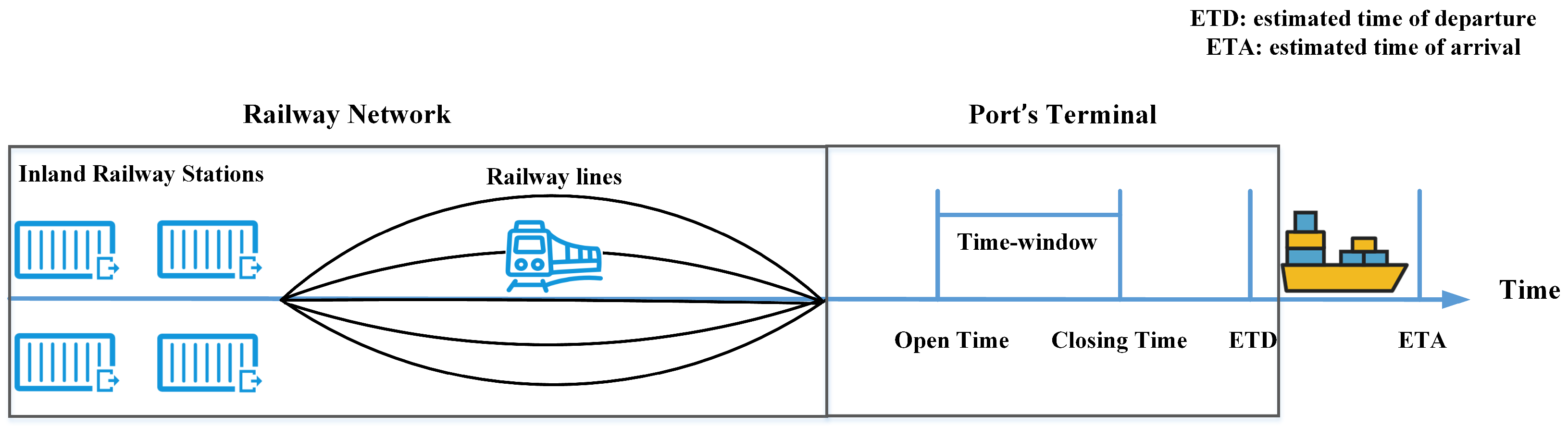
- Seaport’s collection time window: As rail-sea intermodal integration is a key feature of the corridor, a time window constraint is imposed at the seaport. All demands terminate at the seaport and must meet this constraint. On one hand, the port provides a certain amount of free storage time, typically related to the shipping schedule [41]. On the other hand, the railway arrival times must be coordinated as closely as possible with the shipping schedule [7]. As shown in Figure 2, if a train arrives within the designated time window, no storage cost is incurred; otherwise, additional storage waiting time is required. This constraint is unique to intermodal-based train operations in SHCs.
- Selecting a service from the set of potential train service patterns for each city.
- Defining each train’s arrival and departure timings, as well as its route, in accordance with its service pattern. Note that the departure time in this study is focused on coordinating operations between rail and sea transport; it serves as a macro-level outline rather than a detailed timetable.
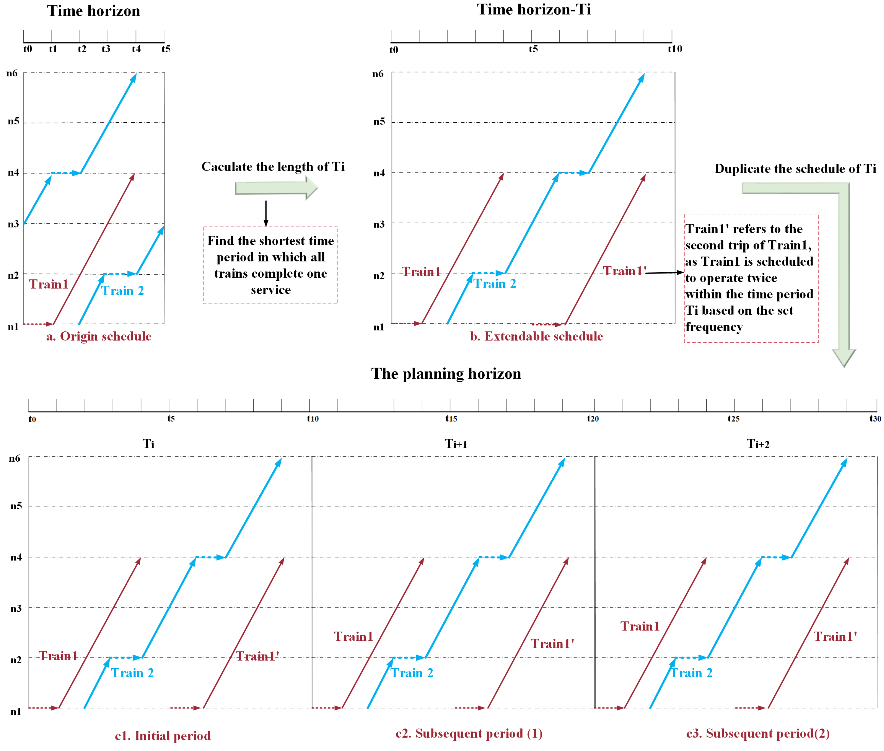
- Specifying the frequency of each train service within the planning horizon. Due to this frequency requirement, identical trains must be scheduled at evenly spaced intervals throughout the planning horizon.
3.2. Notation and Definition
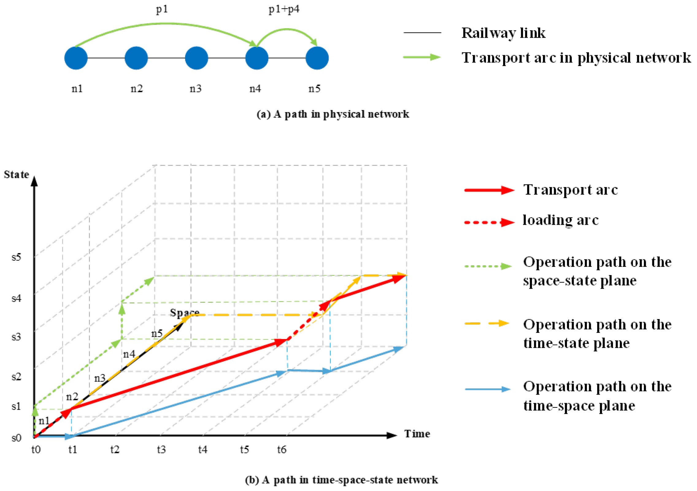
3.3. Time-Space-State Network Formulation
4. Model Formulation
4.1. Modeling Approach
4.2. Modeling Assumptions
- Assume that the time, space, and quantity of demands are known. In this context, demands refer to customer cargo transport requirements, calculated by containers. This is a common assumption in deterministic rail service planning studies, as these data represent key parameters.
- To maintain competitive advantage, it is assumed that each train service makes no more than one stop during its journey, as additional stops increase travel time [40].
- To simplify the work of rail operators, we assume that the planning horizon is a week and the time step is an hour. When demand fluctuates weekly or seasonally, this fixed planning horizon can be handled using a rolling or periodic approach, where the model is updated regularly to reflect the latest demand patterns.
- The scheduled train services are planned to operate at regular intervals [44].
- Given the ongoing infrastructure improvements, we assume that the capacity of the rail track, station, and port infrastructure will meet the operational requirements of the proposed train services.
4.3. Objective Function
- if arc is selected by train a in the initial period; otherwise, .
- if arc is selected by train a in subsequent periods; otherwise, .
- represents the frequency of the train a, indicating the number of times the train a operates within the planning horizon.
- denotes the departure time of the train a, specifying when the train a begins its journey on the schedule.
4.4. Constraints
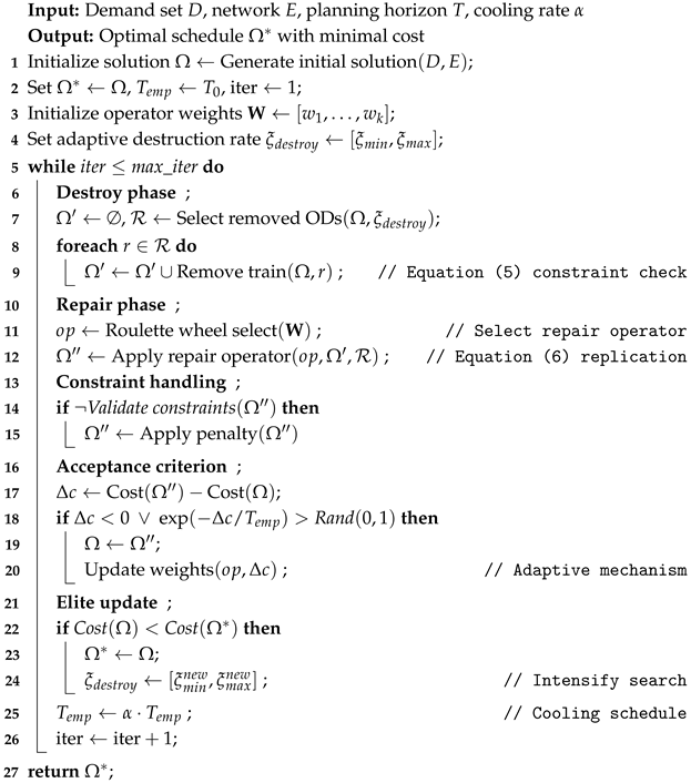
5. Solution Algorithm
| Algorithm 1: Adaptive large neighborhood search for SSND-ST problem |
 |
6. Results and Discussion
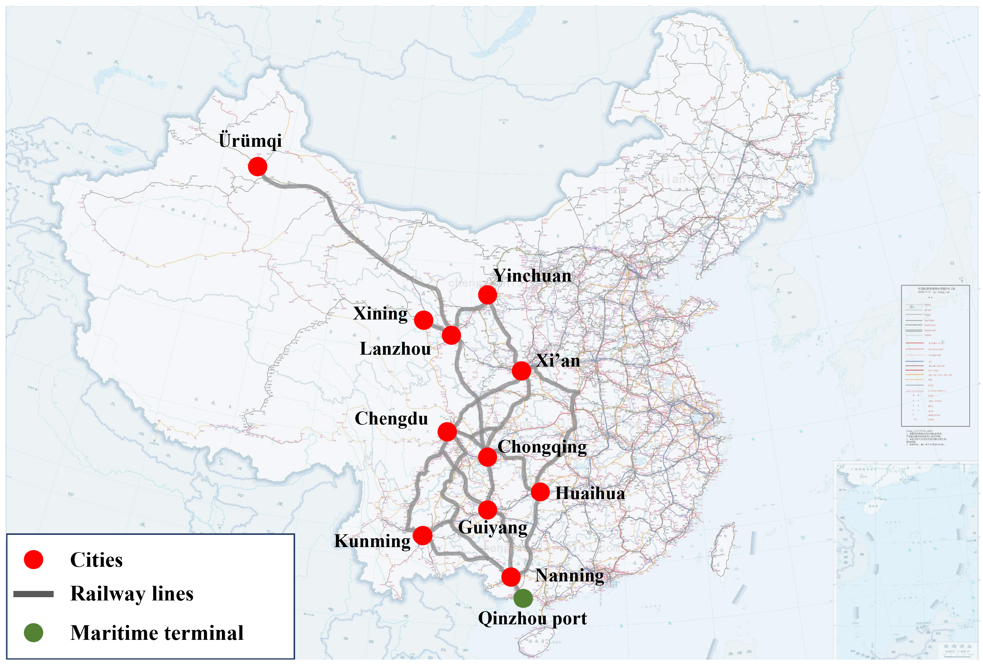
6.1. Case Study
6.2. Result
6.3. Discussion
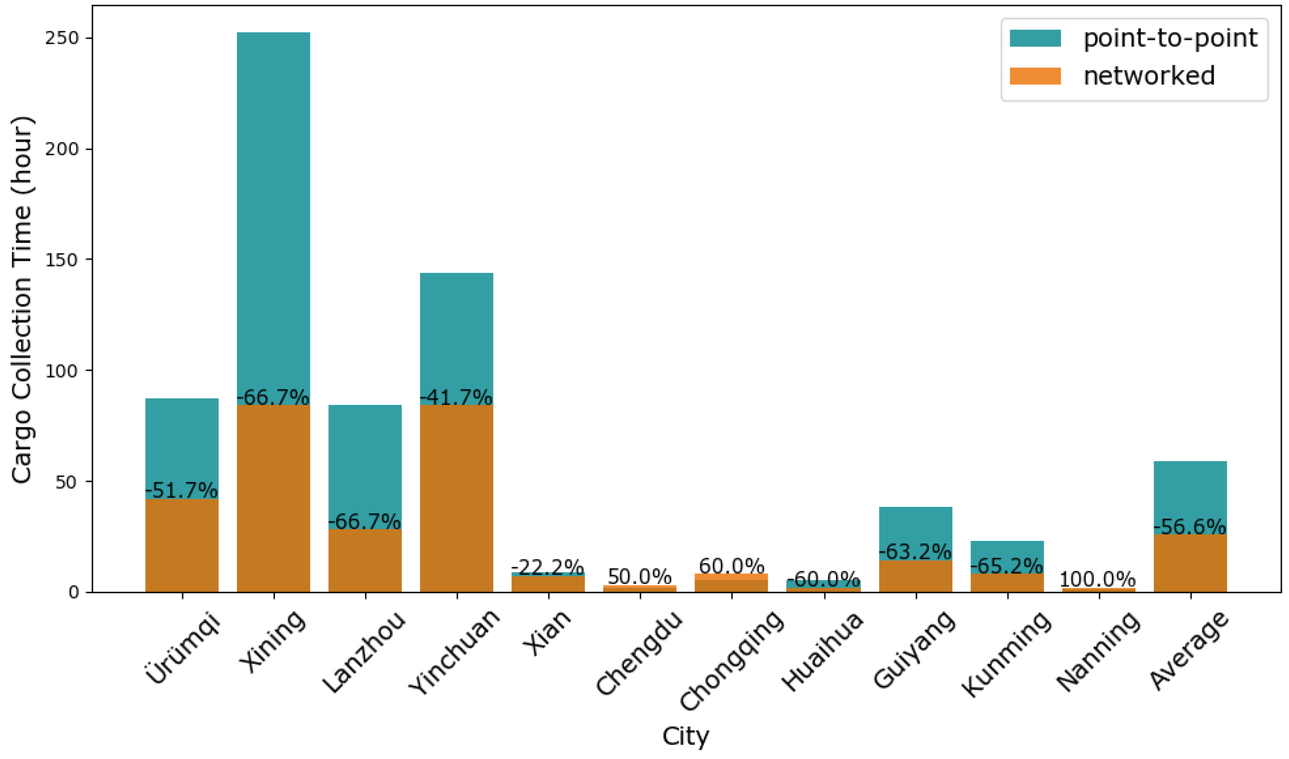
6.3.1. Results Improvement
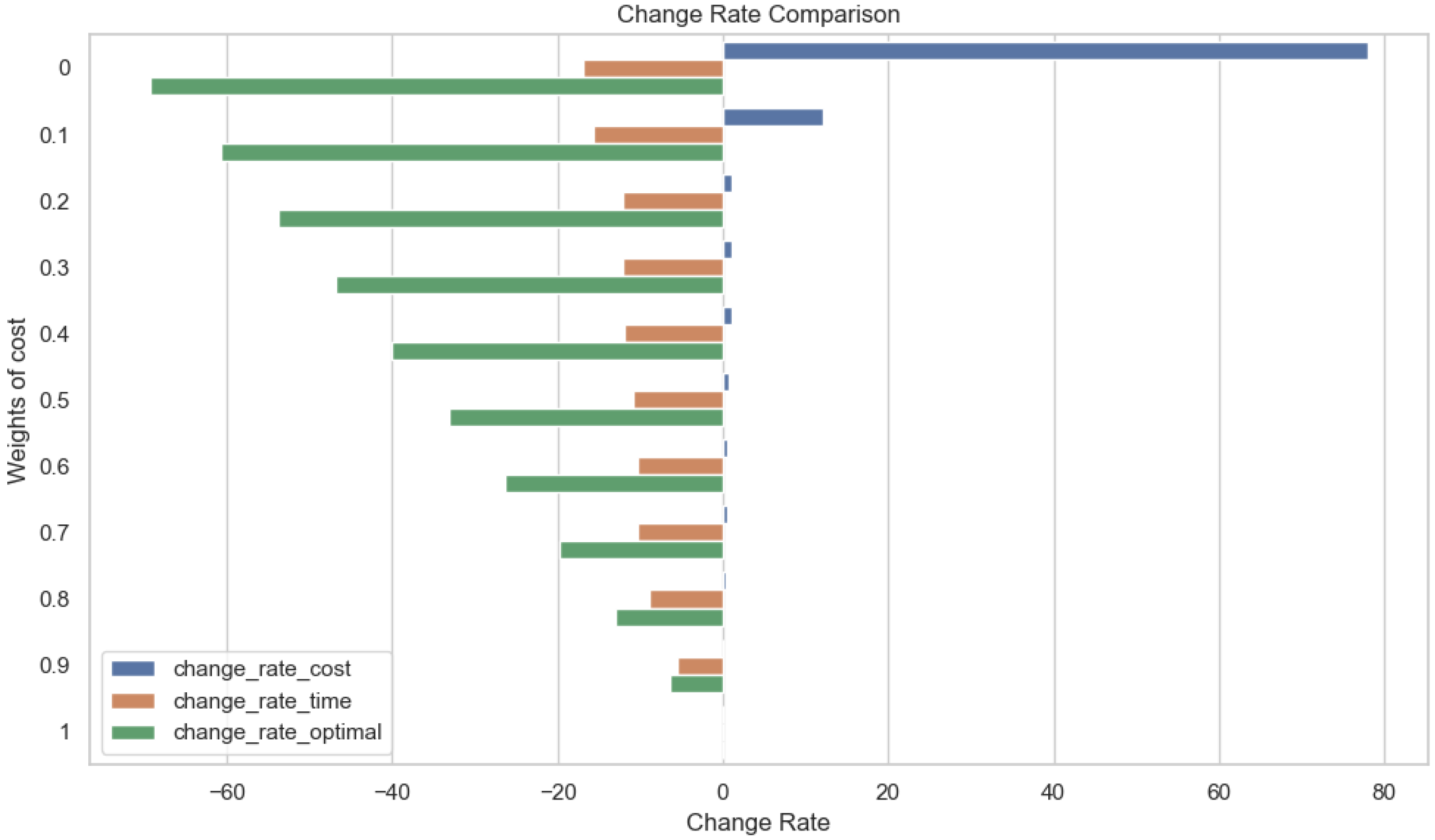
6.3.2. Cost and Time Object
6.3.3. Demand and Capacity Limits
7. Conclusions
Author Contributions
Funding
Data Availability Statement
Conflicts of Interest
References
- Parola, F.; Risitano, M.; Ferretti, M.; Panetti, E. The drivers of port competitiveness: A critical review. Transp. Rev. 2017, 37, 116–138. [Google Scholar] [CrossRef]
- Dalivand, A.A.; Torabi, S.A. Sustainable-resilient seaport-dry port network design considering inter-modal transportation. J. Clean. Prod. 2024, 452, 141944. [Google Scholar] [CrossRef]
- Deng, P.; Song, L.; Xiao, R.; Huang, C. Evaluation of logistics and port connectivity in the Yangtze River Economic Belt of China. Transp. Policy 2022, 126, 249–267. [Google Scholar] [CrossRef]
- Yin, C.; Zhang, Z.; Zhang, X.; Chen, J.; Tao, X.; Yang, L. Hub seaport multimodal freight transport network design: Perspective of regional integration development. Ocean Coast. Manag. 2023, 242, 106675. [Google Scholar] [CrossRef]
- Li, X.; Xie, C.; Bao, Z. A multimodal multicommodity network equilibrium model with service capacity and bottleneck congestion for China-Europe containerized freight flows. Transp. Res. Part E Logist. Transp. Rev. 2022, 164, 102786. [Google Scholar] [CrossRef]
- Kurtuluş, E. Optimizing inland container logistics through dry ports: A two-stage stochastic mixed-integer programming approach considering volume discounts and consolidation in rail transport. Comput. Ind. Eng. 2022, 174, 108768. [Google Scholar] [CrossRef]
- Gao, T.; Tian, J.; Huang, C.; Wu, H.; Xu, X.; Liu, C. The impact of new western land and sea corridor development on port deep hinterland transport service and route selection. Ocean Coast. Manag. 2024, 247, 106910. [Google Scholar] [CrossRef]
- Talley, W.K.; Ng, M. Note: Determinants of cargo port, hinterland cargo transport and port hinterland cargo transport service chain choices by service providers. Transp. Res. Part E Logist. Transp. Rev. 2020, 137, 101921. [Google Scholar] [CrossRef]
- Wang, G.W.; Zeng, Q.; Li, K.; Yang, J. Port connectivity in a logistic network: The case of Bohai Bay, China. Transp. Res. Part E Logist. Transp. Rev. 2016, 95, 341–354. [Google Scholar] [CrossRef]
- Wei, H.; Dong, M. Import-export freight organization and optimization in the dry-port-based cross-border logistics network under the Belt and Road Initiative. Comput. Ind. Eng. 2019, 130, 472–484. [Google Scholar] [CrossRef]
- Wang, L.; Lau, Y.y.; Su, H.; Zhu, Y.; Kanrak, M. Dynamics of the Asian shipping network in adjacent ports: Comparative case studies of Shanghai-Ningbo and Hong Kong-Shenzhen. Ocean Coast. Manag. 2022, 221, 106127. [Google Scholar] [CrossRef]
- Yan, B.; Jin, J.G.; Zhu, X.; Lee, D.H.; Wang, L.; Wang, H. Integrated planning of train schedule template and container transshipment operation in seaport railway terminals. Transp. Res. Part E Logist. Transp. Rev. 2020, 142, 102061. [Google Scholar] [CrossRef]
- Yin, C.; Ke, Y.; Chen, J.; Liu, M. Interrelations between sea hub ports and inland hinterlands: Perspectives of multimodal freight transport organization and low carbon emissions. Ocean Coast. Manag. 2021, 214, 105919. [Google Scholar] [CrossRef]
- Kawachi, K.; Shibasaki, R. How do corridor development and border facilitation policies impact future container transport in inland South Asia?–A network simulation approach. Asian J. Shipp. Logist. 2024, 40, 61–81. [Google Scholar] [CrossRef]
- Sdoukopoulos, E.; Boile, M. Port-hinterland concept evolution: A critical review. J. Transp. Geogr. 2020, 86, 102775. [Google Scholar] [CrossRef]
- El Yaagoubi, A.; Ferjani, A.; Essaghir, Y.; Sheikhahmadi, F.; Abourraja, M.N.; Boukachour, J.; Baron, M.L.; Duvallet, C.; Khodadad-Saryazdi, A. A logistic model for a french intermodal rail/road freight transportation system. Transp. Res. Part E Logist. Transp. Rev. 2022, 164, 102819. [Google Scholar] [CrossRef]
- Saha, R.C. Inland Container Terminal Development to Increase Seaport’s Competitiveness in Bangladesh. J. Marit. Res. 2023, 20, 8–19. [Google Scholar]
- Kawasaki, T.; Loh, Z.T.; Hanaoka, S. Geospatial Transition of Port Hinterland Considering Intermodal Service Frequency: A Case Study in Bangladesh. J. Transp. Geogr. 2023, 108, 103549. [Google Scholar] [CrossRef]
- Mayer, H.M. Some geographic aspects of technological change in maritime transportation. Econ. Geogr. 1973, 49, 145–155. [Google Scholar] [CrossRef]
- Van Klink, H.A.; van Den Berg, G.C. Gateways and intermodalism. J. Transp. Geogr. 1998, 6, 1–9. [Google Scholar] [CrossRef]
- Khaslavskaya, A.; Roso, V. Dry ports: Research outcomes, trends, and future implications. Marit. Econ. Logist. 2020, 22, 265–292. [Google Scholar] [CrossRef]
- Tsao, Y.C.; Thanh, V.V. A multi-objective mixed robust possibilistic flexible programming approach for sustainable seaport-dry port network design under an uncertain environment. Transp. Res. Part E Logist. Transp. Rev. 2019, 124, 13–39. [Google Scholar] [CrossRef]
- Facchini, F.; Digiesi, S.; Mossa, G. Optimal dry port configuration for container terminals: A non-linear model for sustainable decision making. Int. J. Prod. Econ. 2020, 219, 164–178. [Google Scholar] [CrossRef]
- Bedoya-Maya, F.; Calatayud, A. Enhanced port-city interface through infrastructure investment: Evidence from Buenos Aires. Marit. Econ. Logist. 2023, 25, 249–271. [Google Scholar] [CrossRef]
- Behdani, B.; Wiegmans, B.; Roso, V.; Haralambides, H. Port-hinterland transport and logistics: Emerging trends and frontier research. Marit. Econ. Logist. 2020, 22, 1–25. [Google Scholar] [CrossRef]
- Yıldırım, M.S.; Karaşahin, M.; Gökkuş, Ü. Scheduling of the shuttle freight train services for dry ports using multimethod simulation–optimization approach. Int. J. Civ. Eng. 2021, 19, 67–83. [Google Scholar] [CrossRef]
- Gendreau, M. Network Design with Applications to Transportation and Logistics; Routledge: London, UK, 2023. [Google Scholar]
- Meng, L.; Zhou, X. An integrated train service plan optimization model with variable demand: A team-based scheduling approach with dual cost information in a layered network. Transp. Res. Part B Methodol. 2019, 125, 1–28. [Google Scholar] [CrossRef]
- Müller, J.P.; Elbert, R.; Emde, S. Intermodal service network design with stochastic demand and short-term schedule modifications. Comput. Ind. Eng. 2021, 159, 107514. [Google Scholar] [CrossRef]
- Zhu, E.; Crainic, T.G.; Gendreau, M. Scheduled service network design for freight rail transportation. Oper. Res. 2014, 62, 383–400. [Google Scholar] [CrossRef]
- Ford, L.R. Flows in Networks; Princeton University Press: Princeton, NJ, USA, 2015. [Google Scholar]
- Belieres, S.; Hewitt, M.; Jozefowiez, N.; Semet, F. A time-expanded network reduction matheuristic for the logistics service network design problem. Transp. Res. Part E Logist. Transp. Rev. 2021, 147, 102203. [Google Scholar] [CrossRef]
- Yao, Z.; Nie, L.; Yue, Y.; He, Z.; Ke, Y.; Mo, Y.; Wang, H. Network periodic train timetabling with integrated stop planning and passenger routing: A periodic time–space network construct and ADMM algorithm. Transp. Res. Part C Emerg. Technol. 2023, 153, 104201. [Google Scholar] [CrossRef]
- Yin, J.; Pu, F.; Yang, L.; D’ariano, A.; Wang, Z. Integrated optimization of rolling stock allocation and train timetables for urban rail transit networks: A benders decomposition approach. Transp. Res. Part B Methodol. 2023, 176, 102815. [Google Scholar] [CrossRef]
- Ambrosino, D.; Asta, V. An innovative operation-time-space network for solving different logistic problems with capacity and time constraints. Networks 2021, 78, 350–367. [Google Scholar] [CrossRef]
- Wang, X.; Tang, T.; Su, S.; Yin, J.; Gao, Z.; Lv, N. An integrated energy-efficient train operation approach based on the space-time-speed network methodology. Transp. Res. Part E Logist. Transp. Rev. 2021, 150, 102323. [Google Scholar] [CrossRef]
- Zhang, Y.; Peng, Q.; Yao, Y.; Zhang, X.; Zhou, X. Solving Cyclic Train Timetabling Problem through Model Reformulation: Extended Time-Space Network Construct and Alternating Direction Method of Multipliers Methods. Transp. Res. Part B Methodol. 2019, 128, 344–379. [Google Scholar] [CrossRef]
- Mahmoudi, M.; Zhou, X. Finding optimal solutions for vehicle routing problem with pickup and delivery services with time windows: A dynamic programming approach based on state–space–time network representations. Transp. Res. Part B Methodol. 2016, 89, 19–42. [Google Scholar] [CrossRef]
- Guan, Y.; Xiang, W.; Wang, Y.; Yan, X.; Zhao, Y. Bi-level optimization for customized bus routing serving passengers with multiple-trips based on state–space–time network. Phys. A Stat. Mech. Its Appl. 2023, 614, 128517. [Google Scholar] [CrossRef]
- Dong, X.; Li, D.; Yin, Y.; Ding, S.; Cao, Z. Integrated optimization of train stop planning and timetabling for commuter railways with an extended adaptive large neighborhood search metaheuristic approach. Transp. Res. Part C Emerg. Technol. 2020, 117, 102681. [Google Scholar] [CrossRef]
- Leviäkangas, P. Who paid for COVID-19? Income distribution analysis of Finnish seaports. Case Stud. Transp. Policy 2024, 16, 101192. [Google Scholar] [CrossRef]
- Guo, Q.; Yin, C.; Zheng, S. An intermodal transport network planning scheme considering carbon emissions. Energy 2025, 13, 135564. [Google Scholar] [CrossRef]
- Hu, Z.; Wei, Y.; Xu, Y.; Wang, H.; Li, Y.; Xia, Y. Optimization of ticket pricing for high-speed railway considering full competitive environment. Meas. Control 2024, 57, 1358–1369. [Google Scholar] [CrossRef]
- Giusti, R.; Manerba, D.; Crainic, T.G.; Tadei, R. The synchronized multi-commodity multi-service Transshipment-Hub Location Problem with cyclic schedules. Comput. Oper. Res. 2023, 158, 106282. [Google Scholar] [CrossRef]
- Zheng, H.; Sun, H.; Wu, J.; Kang, L. Alternative Service Network Design for Bus Systems Responding to Time-Varying Road Disruptions. Transp. Res. Part B Methodol. 2024, 188, 103042. [Google Scholar] [CrossRef]
- Canca, D.; De-Los-Santos, A.; Laporte, G.; Mesa, J.A. Integrated Railway Rapid Transit Network Design and Line Planning problem with maximum profit. Transp. Res. Part E Logist. Transp. Rev. 2019, 127, 1–30. [Google Scholar] [CrossRef]
- National Development and Reform Commission. Land-Sea Corridor Work in Western Region to Shift into Higher Gear. 2021. Available online: https://english.www.gov.cn/statecouncil/ministries/202109/03/content_WS613159a5c6d0df57f98df946.html (accessed on 7 April 2025).
- Oruangke, P. The impact of international logistics performance on ASEAN trade. Chiang Mai Univ. J. Econ. 2021, 25, 1–16. [Google Scholar]
- Kreutzberger, E.; Konings, R. The challenge of appropriate hub terminal and hub-and-spoke network development for seaports and intermodal rail transport in Europe. Res. Transp. Bus. Manag. 2016, 19, 83–96. [Google Scholar] [CrossRef]
- Muñuzuri, J.; Lorenzo-Espejo, A.; Pegado-Bardayo, A.; Escudero-Santana, A. Integrated Scheduling of Vessels, Cranes and Trains to Minimize Delays in a Seaport Container Terminal. J. Mar. Sci. Eng. 2022, 10, 1506. [Google Scholar] [CrossRef]


| Type | Symbol | Definition |
|---|---|---|
| Sets | N | Set of nodes in the physic network |
| R | Set of links in the physic network | |
| T | Set of time horizon in the network | |
| S | Set of states corresponds to demands and trains in the network | |
| V | Set of TSS vertexes | |
| E | Set of arcs in the TSS network | |
| A | Set of trains | |
| P | Set of demands, denoted by origin and destination nodes, in terms of OD pairs | |
| L | Set of links in space dimension | |
| Set of arcs correspond to train a, | ||
| Set of arcs denoted train a is selected by OD pair p, | ||
| Indexes | i | Index of nodes, |
| t | Index of times, | |
| Index of times in subsequent periods, | ||
| s | Index of state, | |
| a | Index of trains, | |
| p | Index of OD pairs | |
| Initial volume of OD pair p | ||
| Index of time-space-state vertex | ||
| Index of time-space-state arcs, | ||
| Parameters | Origin station of OD pair p | |
| Destination station of OD pair p | ||
| Arrival time of train a at node i | ||
| Departure time of train a at node i | ||
| Storage time of train a at destination | ||
| State of train a when arriving at node i | ||
| State of train a when departing from node i | ||
| The first train a in the initial period | ||
| The order of train a with the same schedule | ||
| Cost of link , | ||
| Transport time of link , | ||
| Capacity of train a | ||
| Time windows of the destination node | ||
| Length of the planning horizon | ||
| Length of the initial period | ||
| Length of the subsequent period | ||
| H | Number of plan periods | |
| Order of subsequent period, | ||
| Variables | =1 if arc is selected, =0 otherwise | |
| =1 if arc is selected, =0 otherwise | ||
| Frequency of train a | ||
| The departure time of train a |
| Instances | GUROBI | ALNS | ||||
|---|---|---|---|---|---|---|
| Weighted Obj. | CPU (s) | Gap | Weighted Obj. | CPU (s) | Gap | |
| 3 cities | 1654 | 52.06 | 0.00% | 1654 | 23.35 | 0.00% |
| 4 cities | 4335 | 368.08 | 0.00% | 4335 | 56.88 | 0.00% |
| 5 cities | 25,145 | 919.86 | 0.00% | 25,159 | 68.56 | 0.06% |
| City | Number | City | Number | City | Number |
|---|---|---|---|---|---|
| Ürümqi | 1 | Chengdu | 6 | Nanning | 11 |
| Xining | 2 | Chongqing | 7 | Qinzhou Port | 12 |
| Lanzhou | 3 | Huaihua | 8 | ||
| Yinchuan | 4 | Guiyang | 9 | ||
| Xi’an | 5 | Kunming | 10 |
| City Number (O–D) | Origin City | Weekly Container Shipping Volume (TEU) |
|---|---|---|
| 1→12 | Ürümqi | 58 |
| 2→12 | Xining | 20 |
| 3→12 | Lanzhou | 60 |
| 4→12 | Yinchuan | 35 |
| 5→12 | Xi’an | 580 |
| 6→12 | Chengdu | 2657 |
| 7→12 | Chongqing | 1017 |
| 8→12 | Huaihua | 936 |
| 9→12 | Guiyang | 133 |
| 10→12 | Kunming | 218 |
| 11→12 | Nanning | 3886 |
| City Number (O–D) | City (OD) | Distance (km) | City Number (O–D) | City (OD) | Distance (km) |
|---|---|---|---|---|---|
| 1–2 | Ürümqi–Lanzhou | 1926 | 5–8 | Xi’an–Huaihua | 837 |
| 2–3 | Xining–Lanzhou | 216 | 5–6 | Xi’an–Chengdu | 842 |
| 3–6 | Lanzhou–Chengdu | 1172 | 6–10 | Chengdu–Kunming | 1100 |
| 3–7 | Lanzhou–Chongqing | 1676 | 6–7 | Chengdu–Chongqing | 504 |
| 4–3 | Yinchuan–Lanzhou | 468 | 7–8 | Chongqing–Huaihua | 708 |
| 4–5 | Yinchuan–Xi’an | 1144 | 9–11 | Guiyang–Nanning | 865 |
| 5–7 | Xi’an–Chongqing | 1346 | 11–12 | Nanning–Qinzhou Port | 173 |
| Parameter | [ET_d, LT_d] | [, ] | |
|---|---|---|---|
| Unit | hour | / | TEU |
| Value | 168 | 12:00–16:00 everyday | [20, 100] |
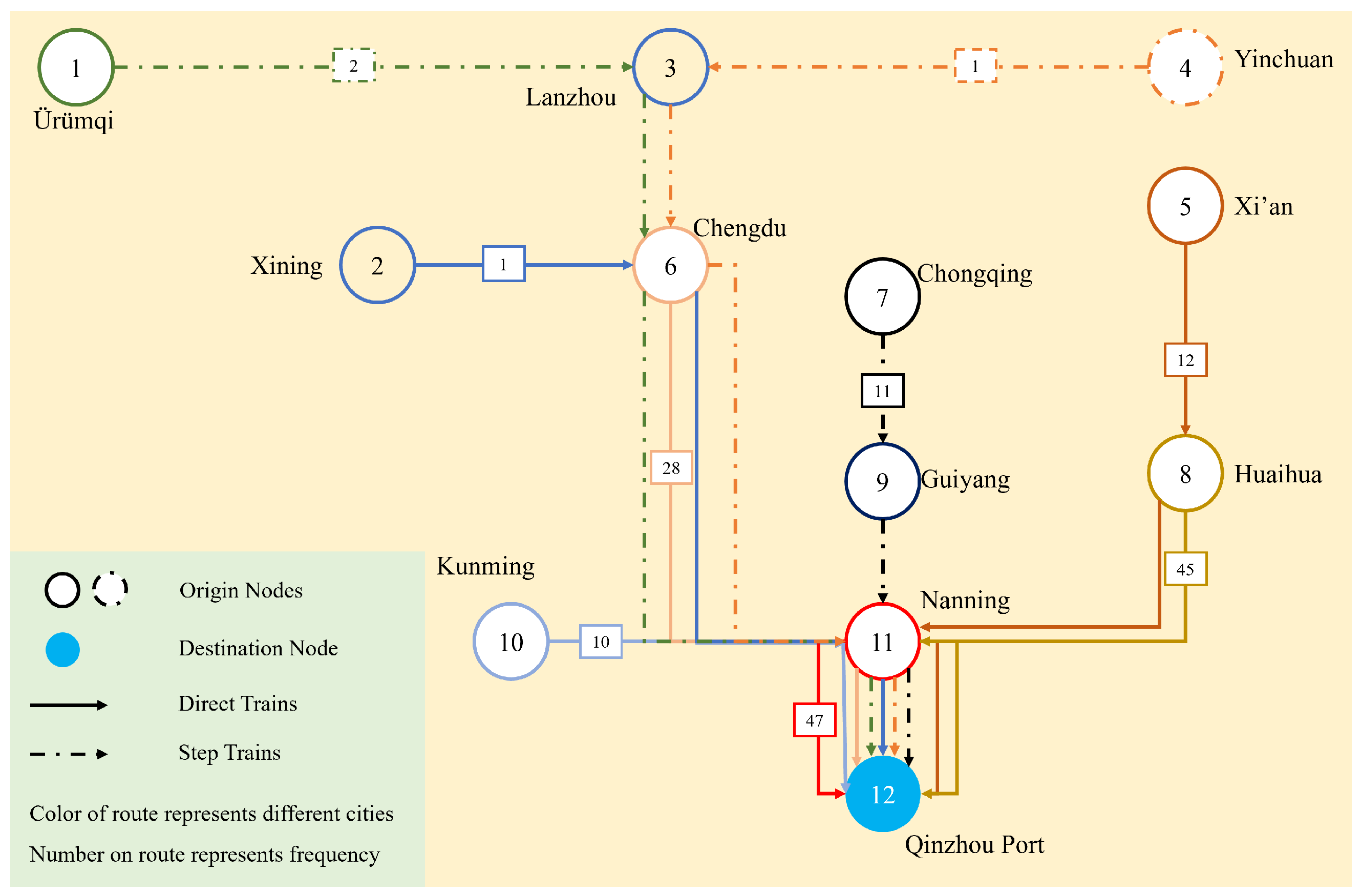
| Type | Original | Departure Day of the First Train | Departure Time of the First Train | Stop City | Frequency |
|---|---|---|---|---|---|
| Direct trains | Xining | Saturday | 10:00 | — | 1 |
| Xi’an | Monday | 14:00 | — | 12 | |
| Chengdu | Monday | 06:00 | — | 28 | |
| Kunming | Monday | 04:00 | — | 10 | |
| Huaihua | Monday | 01:00 | — | 45 | |
| Nanning | Monday | 00:00 | — | 47 | |
| Step trains | Ürümqi | Thursday | 05:00 | Lanzhou | 2 |
| Yinchuan | Thursday | 02:00 | Lanzhou | 1 | |
| Chongqing | Monday | 15:00 | Guiyang | 11 |
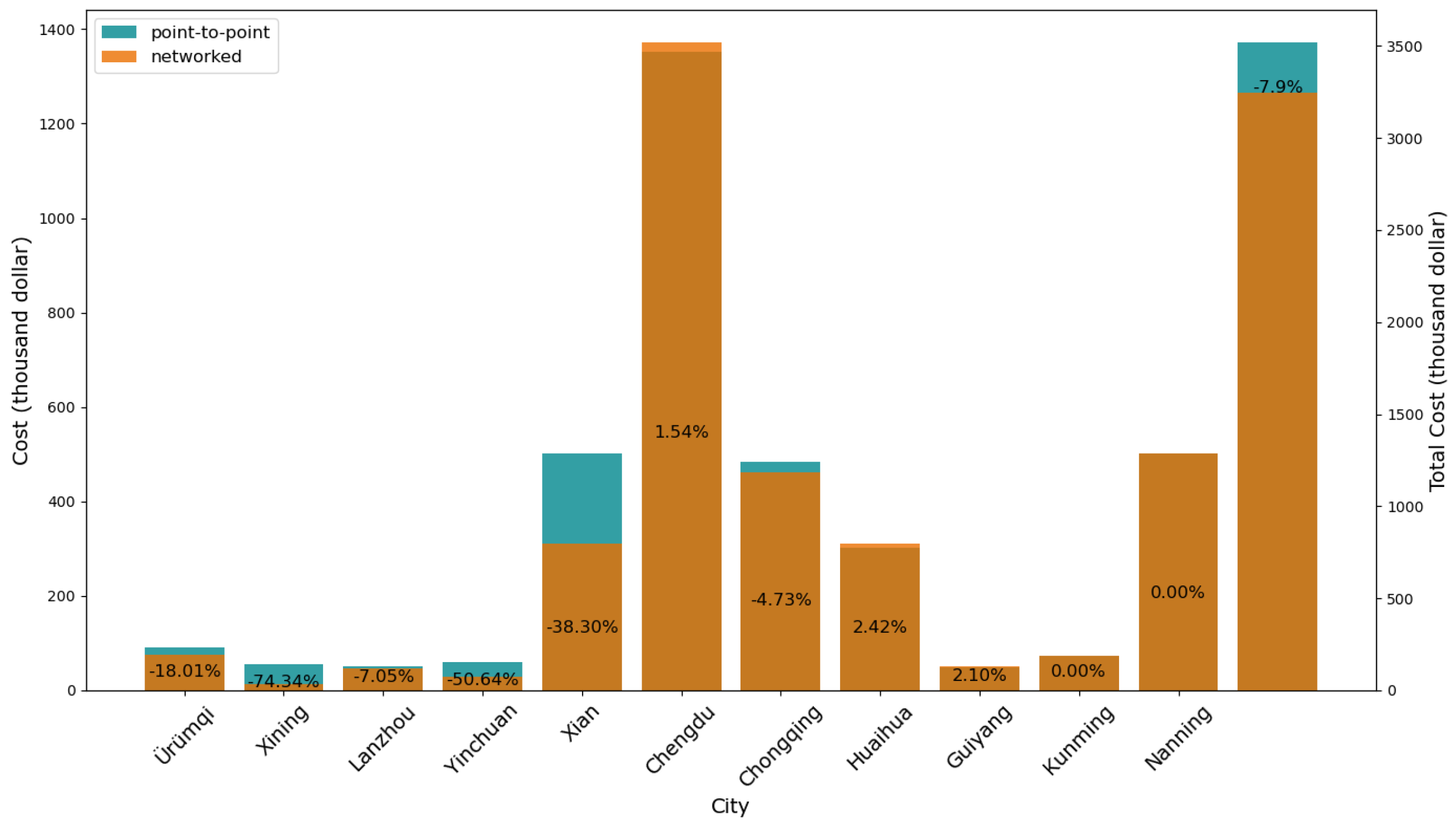
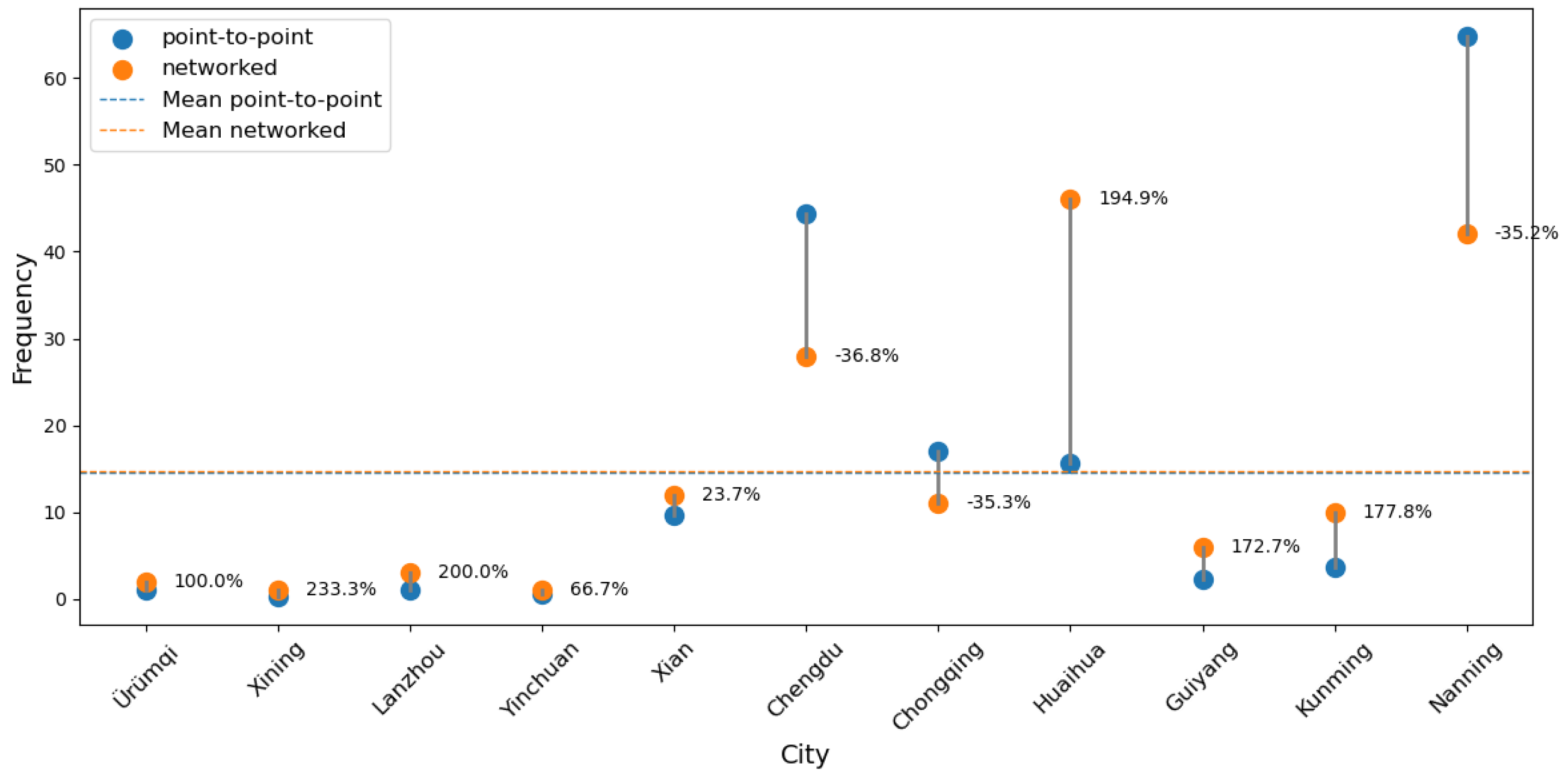
| City | Transport Cost (USD) | Travel Time (h) | Service Frequency | |||
|---|---|---|---|---|---|---|
| Point-to-Point | Networked | Point-to-Point | Networked | Point-to-Point | Networked | |
| Ürümqi | 91,347 | 74,900 | 156 | 91 | 0.5 | 2 |
| Xining | 54,668 | 14,025 | 300 | 103 | 0.3 | 1 |
| Lanzhou | 50,909 | 47,321 | 132 | 57 | 1 | 3 |
| Yinchuan | 59,053 | 29,148 | 183 | 109 | 0.5 | 1 |
| Xi’an | 502,216 | 309,844 | 60 | 27 | 9 | 12 |
| Chengdu | 1,351,377 | 1,372,181 | 36 | 33 | 44 | 28 |
| Chongqing | 486,364 | 460,744 | 36 | 26 | 16 | 11 |
| Huaihua | 302,337 | 309,666 | 16 | 13 | 15 | 45 |
| Guiyang | 49,479 | 50,520 | 60 | 27 | 2 | 11 |
| Kunming | 72,945 | 72,945 | 36 | 20 | 3 | 10 |
| Nanning | 501,294 | 501,294 | 12 | 10 | 64 | 47 |
| Average | 319,933 | 294,781 | 93 | 47 | 14 | 16 |
| City | Networked Service | Point-to-Point Service | Reduction Rate | ||
|---|---|---|---|---|---|
| Arrival Time | Storage Time | Arrival Time | Storage Time | ||
| Chengdu | 31.275 | 4.725 | 23.9 | 12.1 | 61.0% |
| Chongqing | 33.775 | 2.225 | 18.77 | 17.23 | 87.1% |
| Kunming | 15.365 | 0 | 1.28 | 10.72 | 100% |
| Weight of Cost | 0 | 0.1 | 0.2 | 0.3 | 0.4 | 0.5–0.9 | 1.0 |
|---|---|---|---|---|---|---|---|
| Ürümqi | step | step | step | step | step | direct | step |
| Xining | step | step | step | direct | direct | direct | step |
| Lanzhou | step | step | step | step | step | direct | step |
| Yinchuan | step | step | step | step | step | direct | step |
| Xi’an | direct | direct | direct | direct | direct | direct | step |
| Chengdu | step + direct | direct | direct | direct | direct | direct | step |
| Chongqing | step + direct | step + direct | step + direct | step + direct | direct | direct | step |
| Huaihua | direct | direct | direct | direct | direct | direct | step |
| Guiyang | step | step | step | step | direct | direct | step |
| Kunming | direct | direct | direct | direct | direct | direct | step |
| Nanning | direct | direct | direct | direct | direct | direct | step |
Disclaimer/Publisher’s Note: The statements, opinions and data contained in all publications are solely those of the individual author(s) and contributor(s) and not of MDPI and/or the editor(s). MDPI and/or the editor(s) disclaim responsibility for any injury to people or property resulting from any ideas, methods, instructions or products referred to in the content. |
© 2025 by the authors. Licensee MDPI, Basel, Switzerland. This article is an open access article distributed under the terms and conditions of the Creative Commons Attribution (CC BY) license (https://creativecommons.org/licenses/by/4.0/).
Share and Cite
Li, Y.; Zhang, X. Optimizing Scheduled Train Service for Seaport-Hinterland Corridors: A Time-Space-State Network Approach. Mathematics 2025, 13, 1302. https://doi.org/10.3390/math13081302
Li Y, Zhang X. Optimizing Scheduled Train Service for Seaport-Hinterland Corridors: A Time-Space-State Network Approach. Mathematics. 2025; 13(8):1302. https://doi.org/10.3390/math13081302
Chicago/Turabian StyleLi, Yueyi, and Xiaodong Zhang. 2025. "Optimizing Scheduled Train Service for Seaport-Hinterland Corridors: A Time-Space-State Network Approach" Mathematics 13, no. 8: 1302. https://doi.org/10.3390/math13081302
APA StyleLi, Y., & Zhang, X. (2025). Optimizing Scheduled Train Service for Seaport-Hinterland Corridors: A Time-Space-State Network Approach. Mathematics, 13(8), 1302. https://doi.org/10.3390/math13081302