Federated-Learning-Based Strategy for Enhancing Orbit Prediction of Satellites

Abstract

As the primary public source of satellite trajectory data, the Two-Line Element (TLE) dataset offers fundamental orbital parameters for space missions. However, for satellites with poor data quality, traditional neural network models often underperform, hindering accurate orbit predictions and meeting demands in satellite operation and space mission planning. To address this, a federated-learning-based trajectory prediction enhancement strategy is proposed. Satellites with low training efficiency and similar orbits are grouped for collaborative learning. Each satellite uses a Convolutional Neural Network (CNN) model to extract features from historical prediction error data. The server optimizes the global model through the Federated Averaging algorithm, learning more orbital patterns and enhancing accuracy. Experimental results confirm the method’s effectiveness, with a marked increase in prediction accuracy compared to traditional methods, validating federated learning’s advantage. Moreover, the combination of federated learning with basic neural network models like the Multi-Layer Perceptron (MLP), Long Short-Term Memory (LSTM), Recurrent Neural Network (RNN), and Gated Recurrent Unit (GRU) is explored. The results indicate that integrating federated learning can greatly enhance satellite prediction, opening new possibilities for future orbital prediction and space technology development.

1. Introduction

In today’s space environment, the surging number of resident space objects (RSOs) has complicated the space situation. In February 2009, an American Iridium Compass collided with a Russian Cosmos 2251 Compass [1], creating a lot of space debris. In 2021, two SpaceX “Starlink” satellites successively neared the Chinese space station, prompting the Chinese space station complex to conduct emergency collision avoidance maneuvers on 1 July and 21 October. These incidents highlight that with the RSO boom, the risk of satellite conflicts and those involving other space objects has soared. Thus, the global need for effective SSA technology has become more urgent than ever, and enhancing effective space situational awareness (SSA) technology is urgently needed. At the heart of this technology lies the accurate prediction of space object trajectories. Traditional orbit prediction methods, which are based on physical models [2,3], require extensive information about space objects and are costly, often resulting in unsatisfactory predictions. In contrast, machine learning has shown significant potential in many fields, offering a promising solution to the challenge of satellite orbit prediction. By leveraging data-driven models, machine learning can extract patterns from vast datasets and optimize decision-making processes, thereby improving prediction accuracy and reducing costs [4].

Machine learning has recently achieved notable breakthroughs in orbit prediction for space objects based on the TLE dataset, significantly enhancing the accuracy of predictions. Peng et al. conducted extensive research in the field of artificial neural networks, explored the application of SVM in satellite orbit prediction, and confirmed the substantial potential of machine learning for orbit prediction. Their work also demonstrated the generalization capability of this approach in three key areas: time, cross-task, and future predictions [4,5]. Li et al. highlighted the limitation that the accuracy of orbit predictions using TLE and Simplified General Perturbations 4 (SGP4) propagators rapidly decreases over time. They proposed the use of two state-of-the-art learning methods, Gradient-Enhanced Decision Trees (GBDT) and CNN, to model error patterns and use the learned models as error correctors for future orbital predictions. This led to a more than 75% improvement in track prediction accuracy, showcasing the significant potential of machine learning to enhance SSA capabilities [6]. Ferrer et al. developed supervised learning models based on Kepler and SGP4 orbital models to predict Inter-Satellite Links. Their study demonstrates how orbital data can improve Inter-Satellite Link (ISL) prediction accuracy, thus optimizing link management and space resource utilization in satellite networks [7].

The first two studies propose static prediction models that depend on predefined parameters and assumptions, leading to unstable prediction results as the parameters and assumptions may not accurately capture the complex dynamics of RSO orbits. Li et al. identified a research gap in methods for dynamically adjusting prediction models using real-time orbital data. They proposed a method for dynamically adjusting the loss function during training. By integrating a dynamic loss function into the existing TLE-ML orbit prediction framework, they were able to update model parameters based on real-time data, improving the accuracy and adaptability of RSO orbit predictions over time. Their approach increased the accuracy of predictions for the next 14 days by more than 90% [8], which is of significant importance for applications that depend on accurate RSO orbit predictions.

Although the accuracy of orbit prediction methods has been continuously improving, it is evident that these methods are not universally applicable to all satellites. Certain satellites still pose challenges for accurate orbit prediction due to the presence of anomalies in their data or the high complexity of their orbits. This paper introduces a distributed machine learning technology, federated learning, which captures shared characteristics of multi-party data through model migration. In the federated learning process, a central server coordinates the joint training of multiple clients. Each client conducts personalized training based on its local data to generate a local model. Upon completion of training, each client sends updates to the central server, and the server applies the client parameters to the global model using the Federated Averaging algorithm (FedAvg). The updated global model is then distributed back to each client for further local training combined with their respective data. This iterative process is repeated multiple times, ultimately yielding a global model that generalizes well across all clients, learning the unique characteristics of each while maintaining global adaptability [9]. McMahan et al. proposed the FedAvg algorithm, demonstrating how efficient deep learning training can be conducted on decentralized data without transmitting raw data, significantly reducing communication overhead [10]. Simultaneously, this method has shown promising results in terms of model accuracy and convergence speed. In recent years, federated learning has been widely applied in fields such as intelligent transportation [11], manufacturing [12], and healthcare [13,14]. Yang et al. used federated learning to train a model to improve the search suggestion function of a virtual keyboard, keeping the user’s data on the local device while ensuring privacy and improving the accuracy and quality of search suggestions [15]. By combining decentralized federated learning (DFL) for satellite image super-resolution (SR), which improves data quality, Zhao et al. used personalized federated learning (PFL) to process heterogeneous data features and adopted model pruning to reduce complexity, significantly improving the in-orbit training efficiency and model adaptability of low-orbit satellite constellations [16]. These studies demonstrate the feasibility of federated learning in multiple fields. Leveraging the unique characteristics of federated learning, we apply it to satellite orbit prediction, aiming to drive innovation and breakthroughs in this field.

Compared with previous studies, our research focuses on satellites with low prediction accuracy caused by data deficiency or data redundancy. Since data from different sources are not shared in real scenarios, we hope to use data from diverse sources to conduct collaborative modeling so as to improve the prediction accuracy. In the following sections, Section 2 will provide a detailed overview of the experimental data and model, with a focus on explaining the algorithmic details of the organic integration of CNN and federated learning. Section 3 presents the experimental results of the FL–CNN model. Section 4 discusses the practical effects of combining federated learning with models such as MLP, LSTM, RNN, and GRU, and explores the feasibility boundaries of federated learning in satellite orbit prediction research. Finally, in the Section 5, we summarize the research findings, candidly analyze the limitations and shortcomings of the study, and propose directions for future research.

2. Materials and Methods

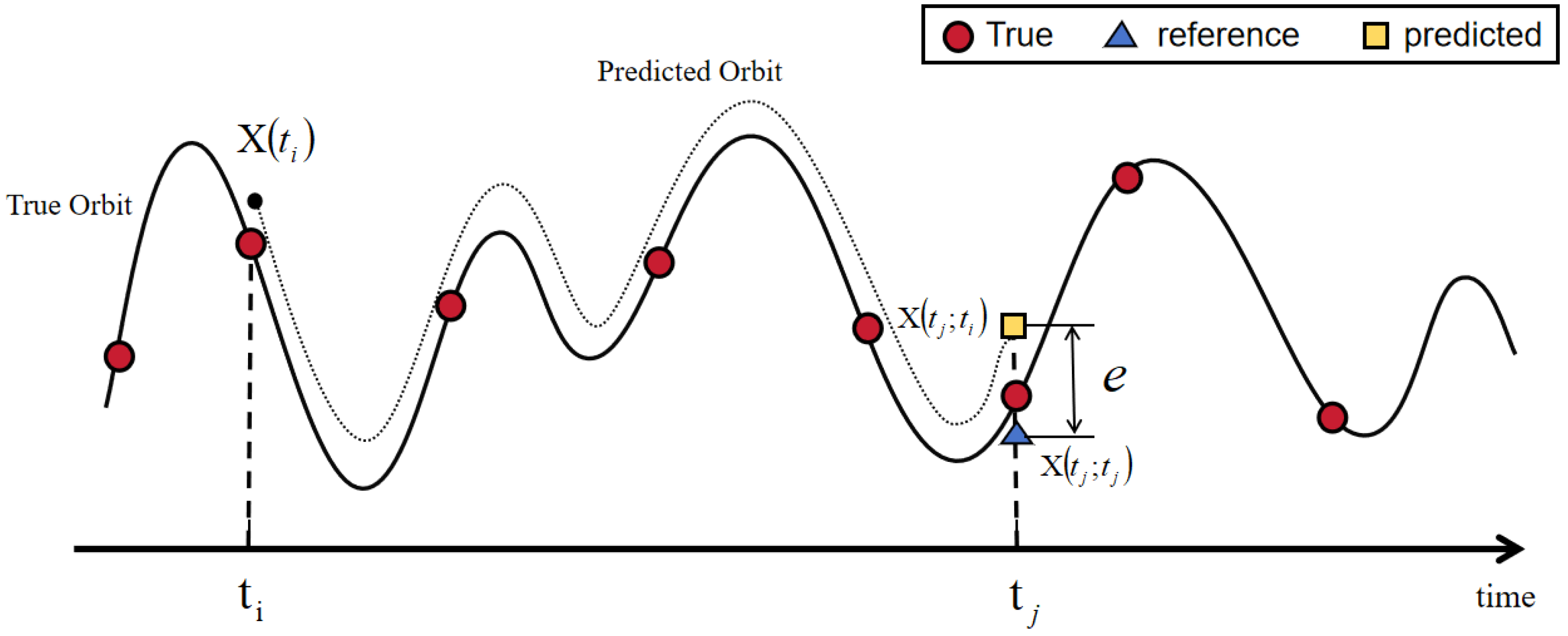
2.1. Data Description

In deep learning, input data serve as the foundation for model learning and prediction. High-quality input data not only enhance the accuracy of the model, but also improve its stability and generalization capabilities.

Satellite orbit prediction involves calculating the future position and velocity of a satellite in orbit based on known orbital data and physical laws. In this paper, we adopt the TLE data processing method proposed by LiBin [6], utilizing publicly available Two-Line Element (TLE) data provided by the North American Aerospace Defense Command (NORAD) as the orbital dataset (data source: http://www.space-track.org/ (accessed on 9 November 2024)). The SGP4 propagator is employed to compute and predict the orbits of space objects. The SGP4 model incorporates perturbation factors such as atmospheric density, solar radiation pressure, and atmospheric drag, and processes TLE data using simplified perturbation theory to calculate the satellite’s orbital position at a specific time. This approach yields highly accurate results with low computational and time costs. Using existing observational data, this method provides more accurate short-term orbit predictions. In orbit prediction, the reference epoch is a specific moment used in Two-Line Element (TLE) data to determine the orbital parameters of a satellite. Orbital elements such as the semi-major axis, eccentricity, and the atmospheric drag coefficient in TLE data are determined based on this moment. Since the orbit prediction errors obtained around the reference epoch are relatively small (this is mainly because the orbital state is directly fitted based on the observation data at this moment, and the extrapolation time approaches zero. The cumulative effects of atmospheric drag, errors in the perturbation force model, and residuals of data fitting have not yet been significant [17]), the predicted state within the orbital period centered on the epoch can be regarded as an approximate value of the precise orbit [18]. Therefore, the prediction error can be considered as the difference between the predicted orbital state quantity and the reference orbital state quantity within a specific epoch.

$$e={\widehat{X}}_{pred}-X_{true}.$$

(1)

According to this important property of TLE-OP, we select the TLE data of the jth epoch as the reference epoch and obtain the predicted state vector of this epoch as an approximation of the true state vector, and the error set is obtained within a prediction time range of length T (T is the orbital period) centered on the corresponding calendar element of this data.

Divide this time into n parts, corresponding to n + 1 time points and TLE data

$$t_{j,k}=t_j-{\displaystyle \frac{T}{2}}+k{\displaystyle \frac{T}{n}},k=0,1,2,\dots ,n.$$

(2)

The prediction state vector is obtained by taking the ith TLE data (i < j, $i\in [t_j-{\displaystyle \frac{T}{2}},t_j+{\displaystyle \frac{T}{2}}]$) and extrapolating it to all time points in the prediction time range one by one and comparing it with the state vector obtained from the j-th TLE data to obtain the prediction error

$$e={\widehat{X}}_{(j;i)}-X_{\left(j\right)}={\widehat{X}}_{(j,k;i)}-{\widehat{X}}_{(j,,k;j)}.$$

(3)

To better understand the generation of errors, we have drawn a schematic diagram of error generation and summarized the important variables to be used in

Table 1. Satellite orbital parameters.

NORAD ID	Object Type	Year	Eccentricity	Inclination [deg]	Period [min]	Perigee [km]
17717	DEBRIS	1970	0.9786	99.98	712	600
17795	DEBRIS	1982	0.1059	65.84	1084	989
17806	DEBRIS	1982	0.1043	65.83	1005	919
17588	ROCKET BODY	1987	0.1147	82.57	1471	1410
23233	PAYLOAD	1994	0.1017	98.83	847	832
30035	DEBRIS	1999	0.1003	99.36	853	689
29980	DEBRIS	1999	0.1025	98.57	940	811
45863	PAYLOAD	2020	0.0011	0.06	35,800	35,773
38922	DEBRIS	2012	0.1227	50.05	3340	260

Data source: http://www.space-track.org/ (accessed on 9 November 2024).

. In Figure 1, the j-th moment is the reference epoch. The curve where the red dots are located represents the true orbit of the satellite (True Orbit), which is the actual running trajectory of the satellite. However, it is very difficult to accurately obtain its state in practice. Therefore, we use the reference value to approximate the true value, that is, $X(t_j;t_j)$ marked by the blue triangle. It is the orbital state obtained at the moment $t_j$ based on the corresponding TLE data at that moment (its reference epoch). The point $X(t_j;t_i)$ marked by the yellow square is on the predicted orbit (Predicted Orbit). It is the prediction result of the satellite’s orbital state at the moment $t_j$ obtained by using the orbital information at the moment $t_i$ (based on the TLE data) and calculation methods such as the SGP4 propagator, that is, the predicted state vector. The prediction error corresponds to the difference between the yellow square and the blue triangle. In this figure, the graphs of the reference value and the true value do not coincide. This is because there is indeed a certain degree of error between the two. In order to clearly distinguish these two key concepts and prevent users from having visual cognitive confusion, we deliberately presented the two graphs in a staggered position when drawing the figure.

Based on the above process, and considering that the goal of deep learning in this paper is to learn the mapping relationship between orbital eigenvalues and prediction errors, as well as to correct orbital predictions at future times by capturing potential error patterns [8], it can be determined that the output variable of the model is the orbital prediction error at moment i versus moment j (the error is transformed from the geocentric inertial coordinate system to the UNW coordinate system based on the stationary space object). The corresponding input variables are $[\Delta t,x\left(t_i\right),v\left(t_i\right),x(t_j;t_i),v(t_j;t_i),B^{\ast }],$

• $\Delta t$ indicates the difference between the start time and the end time;
• $x\left(t_i\right)$ denotes the initial position vector in ECI coordinates with three directions, $x\left(t_i\right)=[r{i}_x,r{i}_y,r{i}_z]$;
• $v\left(t_i\right)$ denotes the initial velocity vector in ECI coordinates with three directions, $v\left(t_i\right)=[v{i}_x,v{i}_y,v{i}_z]$;
• $x(t_j;t_i)$ denotes the predicted position vector of j obtained based on i, which can also be expressed as $x(t_j;t_i)=[r{(j;i)}_x,r{(j;i)}_y,r{(j;i)}_z]$;
• $x(t_j;t_i)$ denotes the predicted velocity vector of j obtained based on i, which can also be expressed as $x(t_j;t_i)=[v{(j;i)}_x,v{(j;i)}_y,v{(j;i)}_z]$;
• $B^{\ast }$ represents the damping coefficient, taking into account the effect of atmospheric drag effect.

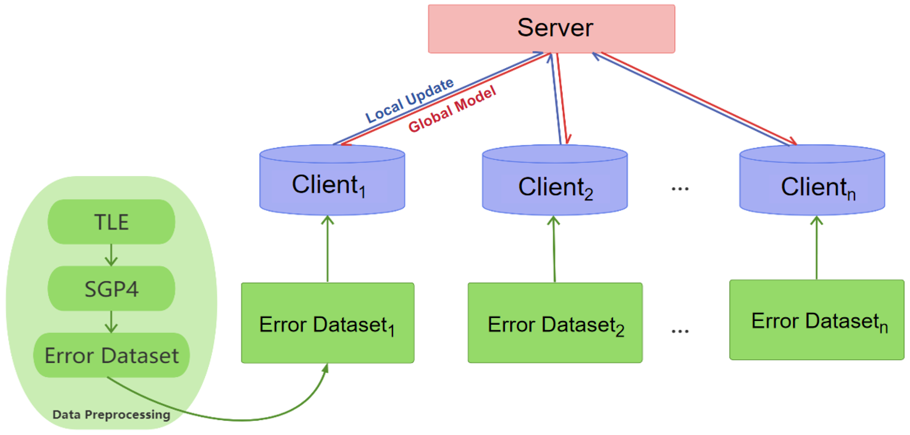
From this, the composition of the dataset can be determined as:

$$D=\{(x_1,y_1),(x_2,y_2),\dots ,(x_n,y_n)\},$$

where $x_i$ is a 14-dimensional vector and $y_i$ is a 3-dimensional vector, corresponding to the input variables at n time points and the target orbital error, respectively.

Due to observation errors and external factors, there may be outliers in the TLE data, which can also lead to outliers in the TLE-OP dataset, necessitating data cleaning. Considering the error growth characteristics of TLE-OP over time, a data cleaning strategy based on the boxplot method is employed to identify outliers [19]. After separating the data points in one-day intervals over the entire prediction time span, the boxplot displays five representative values for each group of data, including the minimum, first quartile ($Q_1$), median ($Q_2$), third quartile ($Q_3$), and maximum. The interquartile range (IQR) is defined as: $IQR=Q_3-Q_1$ is called the interquartile range. An outlier is determined as the data point beyond the outer fence $[Q_1-3\ast IQR,Q_3+3\ast IQR].$ After removing all outliers, the remaining labeled data pairs are considered normal and used for error pattern modeling within the designed Deep Learning (DL) framework.

2.2. Method

A key feature of federated learning is the global adaptability of the global model, meaning that after training, the global model can comprehensively capture the features of each client’s data. During the data analysis phase, we observed that the orbital state vector (input data described in Section 2.1) directly determines the satellite’s orbital dynamics characteristics and, consequently, the results of orbit prediction. For satellites that exhibit poor training performance with ordinary neural network models, we combine an inefficient satellite with several satellites exhibiting similar orbital state vectors for federated learning. This approach enables the global model to better capture the orbital data features of inefficient satellites while leveraging the data from similar satellites to improve prediction accuracy. As a result, the overall performance of orbit prediction is enhanced.

Orbit prediction is intrinsically a regression problem. Its core objective is to leverage models to learn from historical prediction error datasets, thereby enabling accurate assessment of errors at future time points. In the context of federated learning, overly complex network architectures often negatively impact the convergence efficiency of the learning process [20]. In this study, a CNN model based on one-dimensional convolution is proposed. The model is structured sequentially with three convolutional layers, three activation layers, three pooling layers, and two fully connected layers. This well-designed architecture ensures that the model possesses sufficient learning capacity while avoiding efficiency issues associated with excessive complexity. The model effectively extracts key features from historical prediction error data and accurately captures local patterns and temporal characteristics in time-series data, laying a robust foundation for subsequent precise prediction tasks.

In this paper, we adopt the Stochastic Gradient Descent (SGD) method for model [21]. In this approach, only a single batch gradient calculation is performed during each round of client–server communication. To ensure that each global model update incorporates comprehensive data from all participating clients, a synchronization algorithm is used.

In the federated learning setup, n denotes the number of clients, which corresponds to the number of satellites participating in the training process. Each client’s local dataset consists of the data specific to a particular satellite. During training, each client inputs its dataset into the local CNN model to compute the predicted values and the Mean Squared Error. The error gradient is then calculated and propagated backward layer-by-layer to update the weights and biases. Each client model updates the model parameters locally using SGD to complete a step of gradient descent, and then the server weights and averages all the obtained client models and combines the knowledge learned by all clients in their local data to obtain a new global model. The mathematical formula for this process is as follows:

$$g_k={\displaystyle \frac{1}{n}}\nabla F_k\left(w_t\right),$$

(4)

$$w_{t+1}\leftarrow w_t-\eta \sum _{k=1}^K{\displaystyle \frac{n_k}{n}}{g}_k,$$

(5)

where $w_t$ is the parameter of the t-th iteration of the global model, $F_k$ is the loss function corresponding to client K, $g_k$ is the gradient of the loss function $F_k\left(w_t\right)$ with respect to the global model parameter $w_t$ on client K, $\eta$ is the fixed learning rate, and $n_k$ is the number of data pairs in the K-th client.

Before proceeding to the weighted average step, the local update can be iterated several times to optimize the local model based on the client’s local data, allowing the client to better fit its data to improve the local model.The flowchart is shown in Figure 2.

3. Results

In this experiment, a total of four RSOs were selected as experimental subjects. Each of these four satellites was jointly trained through personalized federated learning with two satellites in similar states. A total of nine satellites were used in the experiment. The relevant information is shown in Table 1. The table contains the average values of orbital inclination, eccentricity, and orbital period for a given year obtained from all TLE data. The first 60 days of TLE data are used to create the error dataset for training purposes. The TLE data from day 61 were then used to make updated orbit predictions for the following 14 days (days 61 to 74). These updated predictions were used as new inputs to assess the performance of the trained deep learning model in improving future orbit predictions.

We divided the satellites into four groups, each group consisting of three satellites (30035, 29980, 38922), (30035, 29980, 23233), (17588, 17806, 45863), and (17795, 17806, 17717). The satellites within the same group participated in the federated learning process as clients. For example, the group (30035, 29980, 38922) included satellites 30035, 29980, and 38922, which acted as the first, second, and third clients, respectively. The three satellites jointly optimize the global model parameters. The satellites marked in bold are those whose prediction performance was poor under the ordinary neural network but have significantly improved prediction accuracy after federated learning. This is because when the model was trained on the other two satellites with similar states, it learned the favorable patterns for this satellite, thereby achieving an improvement in prediction accuracy. During the grouping process, we carefully considered both the similarities and differences in satellite orbital parameters. For instance, in some groups, key orbital indicators such as inclination, eccentricity, and perigee height were highly similar between two satellites (e.g., 30035 and 29980, 17806 and 17795). This similarity allowed the model to quickly grasp typical orbital characteristics and establish a foundational understanding based on shared features. Meanwhile, some groups intentionally included one satellite with distinct differences in certain parameters (e.g., 38922 and 45863, which exhibit variations in orbital period or inclination). This design helped prevent model homogenization, enabling the model to better capture the complex and dynamic nature of satellite orbital patterns, thereby enhancing its adaptability and generalization capability across diverse orbital states.

3.1. Experimental Evaluation Metrics

When it comes to evaluating the accuracy of orbital regression predictions, common metrics each have their drawbacks. Mean Squared Error (MSE) is significantly affected by outliers. Mean Absolute Error (MAE) struggles to emphasize large-magnitude errors. Root Mean Squared Error (RMSE) is likewise sensitive to outliers. Furthermore, Mean Absolute Percentage Error (MAPE) becomes unstable when true values approach zero. In order to intuitively evaluate the performance of the error model trained by the machine learning method, this paper uses a model metric. The output of the model in this paper is a predicted value $\widehat{e}$ of the orbital error, so the residual can be expressed as:

$$\Delta e=e-\widehat{e}.$$

(6)

Performance Metric (PM) is used to measure the performance of the ML method in improving OP, and the formula is as follows:

$$PM=\left(1-{\displaystyle \frac{RM{S}_{\Delta e}}{RM{S}_e}}\right)\times 100\%,$$

(7)

where $RM{S}_e=\sqrt{{\displaystyle \frac{1}{n}}{\sum }_{k=1}^n{e}_k^2}$, $RM{S}_{\Delta e}=\sqrt{{\displaystyle \frac{1}{n}}{\sum }_{k=1}^n\Delta e_k^2}$, $RM{S}_{\Delta e}$ represents the Root Mean Square of the error variation, and $RM{S}_e$ represents the Root Mean Square of the original error. This formula measures the accuracy in terms of relative proportion, which can avoid the influence caused by the difference in parameter magnitudes, and is suitable for tasks of different scales. Moreover, based on the root-mean-square calculation, it takes into account both the sensitivity to large errors and the consideration of error distribution, achieving a more refined examination of error characteristics and providing a more effective and stable solution for the accuracy evaluation of orbital regression prediction. If $RM{S}_{\Delta e}$ is much smaller than $RM{S}_e$, it indicates that the error variation is small, that is, the machine learning method has effectively reduced the error. Then, the value of $PM$ will approach 100%, indicating that the model performs well to improve the OP. The PM value ranges from $(-\infty ,1]$, where $PM=1$ indicates perfect prediction accuracy, and $PM<1$ indicates the presence of prediction errors. A lower PM value corresponds to poorer model performance. This design ensures that the PM value comprehensively and intuitively reflects the model’s predictive capability in practical applications.

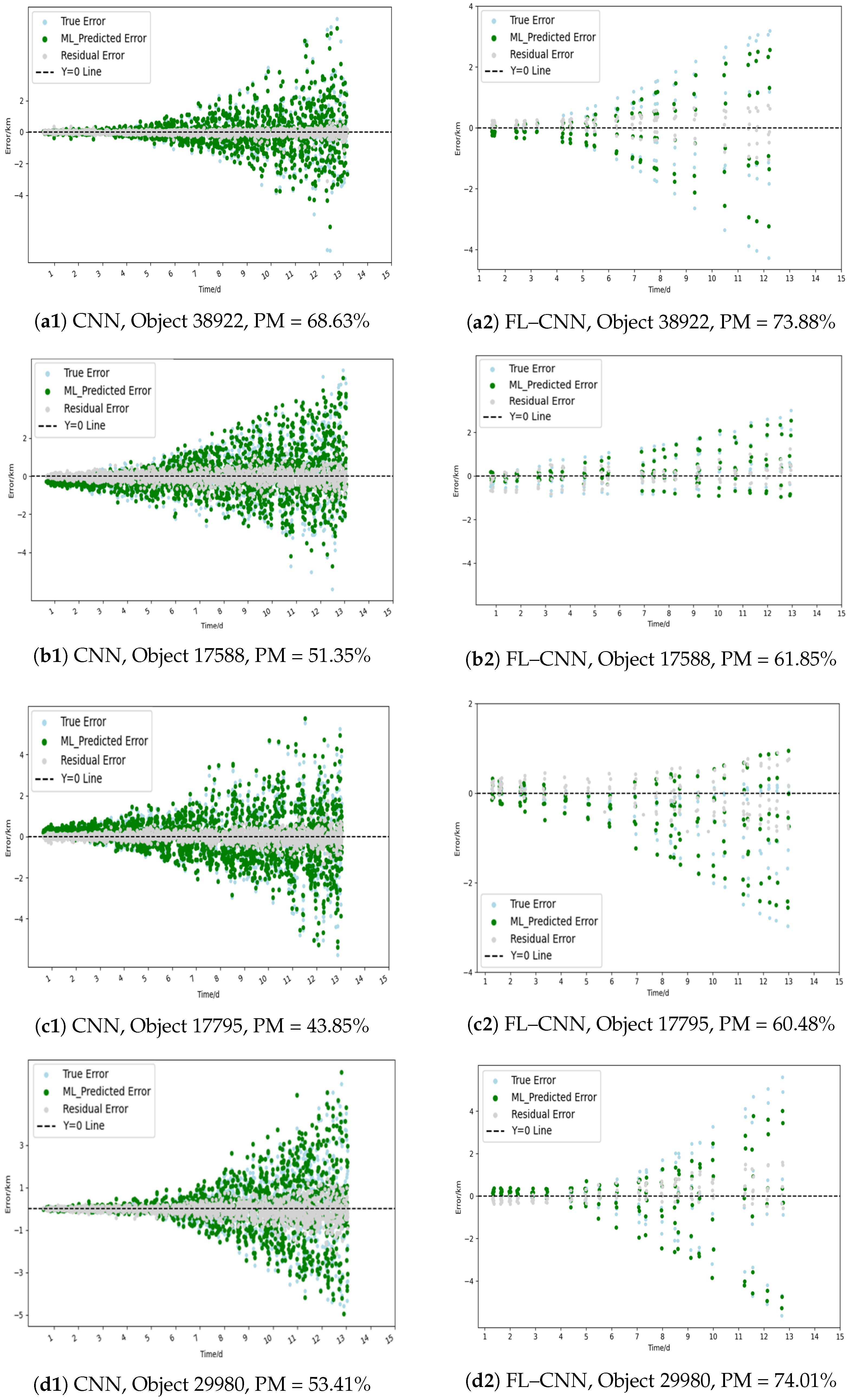
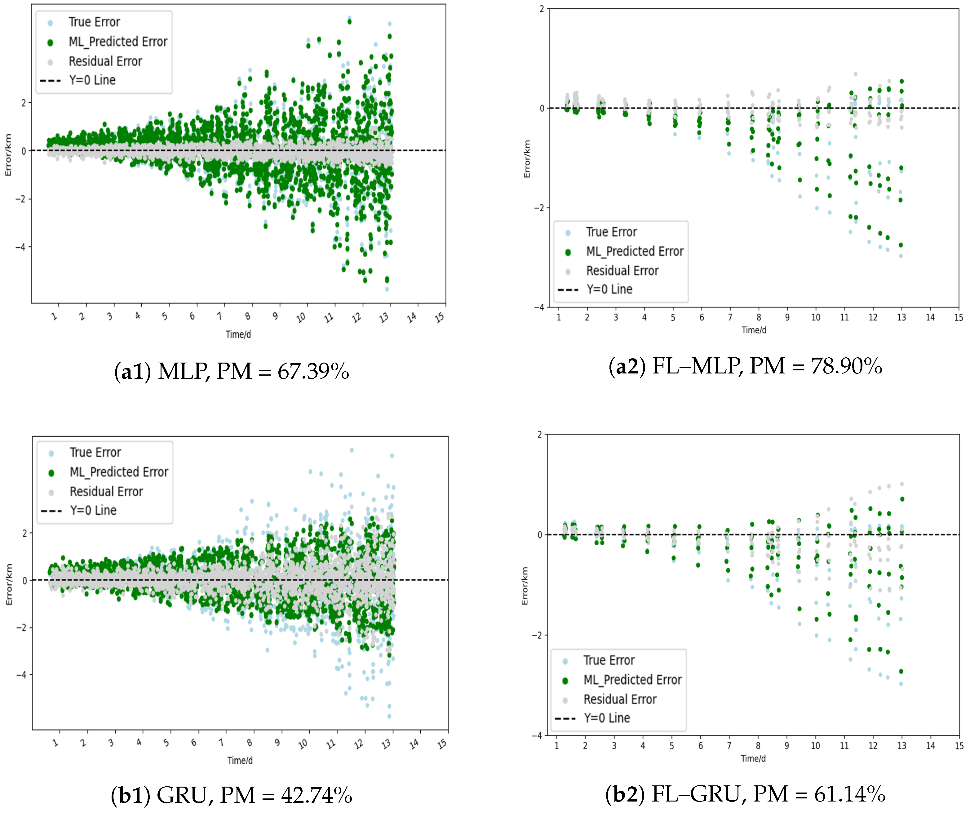
3.2. Performance Comparison

Our approach aims to improve the accuracy and robustness of orbit prediction by integrating CNN models with federated learning to leverage data from similar satellites while training the target satellite model. To validate our methodology, we selected orbital data from four real-world RSOs for experimentation. We conducted 100 rounds of federated learning and compared the performance of the standalone CNN model with the FL–CNN method. The experimental results show that our method improves the accuracy of orbit prediction for satellites with poor performance in the past, especially in the case of complex or unstable satellite orbits, and can achieve more accurate and reliable RSO orbit prediction.

To demonstrate the training effectiveness of the CNN and FL–CNN models, we present time scatter plots of the prediction errors in the W direction for four satellites, visually illustrating the performance differences between the two methods. As shown in Figure 3, each graph has the X-axis representing the forecast time and the Y-axis representing the error. The blue dots represent the real error e (the same as e in Equation (6)), the green dots stand for the prediction error output by the CNN model, and the gray dots indicate the difference between the two, that is, the residual. When the CNN model captures the prediction error effectively, the prediction error aligns closely with the true error, and the residuals approach zero. For these four RSOs, the CNN model struggled to capture the underlying TLE error pattern effectively, resulting in a low PM value. After training, the FL–CNN model demonstrated an improvement of almost 10% over the single model.

The PM values of satellite orbit prediction in other directions are shown in

Table 2. Performance comparison across CNN and FL–CNN.

NORAD ID	${\mathit{PM}}_{\mathit{U}}$		${\mathit{PM}}_{\mathit{N}}$		${\mathit{PM}}_{\mathit{W}}$
	CNN	FL–CNN	CNN	FL–CNN	CNN	FL–CNN
29980	50.45	74.26	68.33	80.43	53.41	85.72
17588	62.00	62.13	51.00	61.85	90.00	76.82
17795	65.54	65.82	65.38	44.21	83.90	85.39
38922	64.22	80.74	73.24	75.10	68.81	74.91

. Across all the satellites tested, the FL–CNN model generally demonstrates better prediction accuracy. Specifically, for satellite 29980, FL–CNN significantly outperforms CNN in all indicators, leading to a marked improvement in prediction accuracy.

4. Discussion

After observing the excellent performance of federated learning (FL) within the CNN framework, we further evaluated its effectiveness by testing it on five other commonly used deep learning models, including MLP, LSTM, and others. Using the orbital data of satellite 17795 in the W direction as an example, we present the scatter plot of its orbital prediction error, as shown in Figure 4. The experimental results for other satellites are summarized in

Table 3. Comparison of satellite prediction accuracy results.

Direction		NORAD ID	29980		17588		17795		38922
	Model
N	MLP/FL–MLP		43.95	83.32	55.05	59.38	67.39	78.90	74.05	77.23
	RNN/FL–RNN		20.41	68.18	61.00	51.17	58.50	65.78	66.24	68.98
	GRU/FL–GRU		22.50	23.54	31.29	45.85	42.74	61.14	9.68	81.58
	LSTM/FL–LSTM		19.24	61.51	53.01	61.15	45.70	58.31	72.01	63.60
	Trans/FL–Trans		35.60	62.79	49.40	45.62	41.73	77.35	40.49	52.27
W	MLP/FL–MLP		41.69	72.37	89.76	49.47	68.47	79.40	77.07	79.59
	RNN/FL–RNN		15.09	69.12	62.78	48.82	75.98	67.95	62.50	65.94
	GRU/FL–GRU		29.98	74.83	61.71	66.15	34.70	76.72	11.49	75.53
	LSTM/FL–LSTM		34.38	72.11	77.09	43.31	76.68	80.52	67.06	81.78
	Trans/FL–Trans		39.97	70.11	70.25	45.52	64.28	47.72	44.17	52.20
U	MLP/FL–MLP		45.68	88.33	68.95	55.93	72.00	50.97	68.73	75.86
	RNN/FL–RNN		23.15	69.94	60.35	71.76	53.08	74.35	67.41	70.18
	GRU/FL–GRU		24.03	28.85	41.82	68.86	23.26	86.19	32.36	84.55
	LSTM/FL–LSTM		34.43	46.18	60.68	53.44	52.85	67.59	72.77	58.93
	Trans/FL–Trans		38.46	54.86	53.91	54.15	28.65	58.48	36.78	68.05

Note: Bold indicates a better training effect for the corresponding model. Trans: Transformer.

.

Through comparative observation, the results show that although the improvement effects of different satellites vary, each model demonstrates performance improvements to varying degrees after personalized federated learning. In addition, while enhancing the model’s performance, this method incurs a relatively low time cost, making it highly efficient.

In this study, a federated learning framework is introduced to optimize the orbit prediction of space targets, successfully improving the prediction accuracy for satellites. Compared with traditional methods, federated learning enhances the adaptability of the model by integrating multi-source data, enabling it to learn more abundant orbital patterns, thus improving prediction efficiency. However, differences in orbital design and satellite types still pose challenges to the model’s performance, especially when data sources and satellite environments vary widely. Future research can further integrate federated fairness to ensure that all data sources contribute fairly to model training and enhance the robustness of federated learning [22], ensuring the model maintains stable and efficient performance in complex environments [23]. It is noteworthy that even with multiple training iterations in the model, a single satellite cannot achieve ideal accuracy levels. However, federated learning enables the satellite to effectively capture favorable patterns when collaborating with other satellites during the federated learning process, thereby improving accuracy. Considering that the time required for neural networks to predict satellite orbits is relatively short, the time cost incurred by iterations remains within an acceptable range. Nevertheless, our experiments revealed that not all collaborative training among seemingly similar satellites yields satisfactory results. While the approach of collaborative training among satellites with orbital similarities is fundamentally viable, the precise methodology for quantifying orbital similarity requires in-depth investigation. To address this challenge, we plan to develop more refined metrics in subsequent experiments to accurately quantify orbital similarity between satellites. Our objective is to better clarify the specific conditions under which collaborative training can effectively optimize the model and maximize prediction accuracy.

In summary, this study advances RSO orbit prediction by introducing a federated learning framework, providing a more accurate and adaptable method for satellites that previously performed poorly. Although challenges remain to adapt to diverse types of satellite, the proposed method lays the foundation for future advancements in orbit prediction technology, with significant potential applications in space security, satellite navigation, and related fields.

5. Conclusions

This paper presents a novel RSO orbit prediction method by integrating personalized federated learning into the traditional TLE-based framework. The method improves the accuracy and adaptability of orbit prediction for inefficient satellites. Experimental results show it outperforms the traditional single-neural-network model, with about a 10% improvement in orbital-direction prediction accuracy for inefficient satellites through error correction. These findings benefit applications relying on precise RSO orbit prediction, such as space debris monitoring and collision avoidance systems. Our study optimizes existing methods and offers a new framework for future satellite orbit prediction. However, the current method has limitations in adapting to different satellite types. Future research could explore more efficient adaptive models to adjust algorithm parameters in various orbital environments. Overall, this research contributes to the RSO orbit prediction methodology and may enhance future prediction accuracy and reliability.

References

1. Kelso, T. Iridium 33/Cosmos 2251 Collision. 2012. Available online: http://celestrak.com/events/collision/ (accessed on 15 February 2017).
2. Montenbruck, O. Numerical integration methods for orbital motion. Celest. Mech. Dyn. Astron. 1992, 53, 59–69. [Google Scholar] [CrossRef]
3. Wang, Y.; Li, M.; Jiang, K.; Li, W.; Zhao, Q.; Fang, R.; Wei, N.; Mu, R. Improving Precise Orbit Determination of LEO Satellites Using Enhanced Solar Radiation Pressure Modeling. Space Weather 2023, 21, e2022SW003292. [Google Scholar] [CrossRef]
4. Peng, H.; Bai, X. Machine Learning Approach to Improve Satellite Orbit Prediction Accuracy Using Publicly Available Data. J. Astronaut. Sci. 2020, 67, 762–793. [Google Scholar] [CrossRef]
5. Peng, H.; Bai, X. Improving orbit prediction accuracy through supervised machine learning. Adv. Space Res. 2018, 61, 2628–2646. [Google Scholar] [CrossRef]
6. Li, B.; Zhang, Y.; Huang, J.; Sang, J. Improved orbit predictions using two-line elements through error pattern mining and transferring. Acta Astronaut. 2021, 188, 405–415. [Google Scholar] [CrossRef]
7. Ferrer, E.; Ruiz-De-Azua, J.A.; Betorz, F.; Escrig, J. Inter-Satellite Link Prediction with Supervised Learning Based on Kepler and SGP4 Orbits. Int. J. Comput. Intell. Syst. 2024, 17, 217. [Google Scholar] [CrossRef]
8. Li, W.; Tao, Y.; Deng, H. Improved Orbit Prediction Method Based on Two-Line Elements with Dynamic Loss Function. EasyChair Prepr. 2025, 15676. [Google Scholar]
9. Chen, X.; Wang, H.; Lu, S.; Yan, R. ALC-PFL: Bearing remaining useful life prediction method based on personalized federated learning. Chin. J. Sci. Instrum. 2023, 44, 69–78. [Google Scholar]
10. McMahan, H.B.; Moore, E.; Ramage, D.; Hampson, S.; y Arcas, B.A. Communication-Efficient Learning of Deep Networks from Decentralized Data. In Proceedings of the 19th International Conference on Artificial Intelligence and Statistics (AISTATS 2016), Cadiz, Spain, 9–11 May 2016; pp. 1273–1282. [Google Scholar]
11. Zhang, R.; Wang, H.; Li, B.; Cheng, X.; Yang, L. A Survey on Federated Learning in Intelligent Transportation Systems. arXiv 2024, arXiv:2403.07444. [Google Scholar] [CrossRef]
12. Pruckovskaja, V.; Weissenfeld, A.; Heistracher, C.; Graser, A.; Kafka, J.; Leputsch, P.; Schall, D.; Kemnitz, J. Federated Learning for Predictive Maintenance and Quality Inspection in Industrial Applications. In Proceedings of the 2023 Prognostics and Health Management Conference (PHM), Salt Lake City, UT, USA, 28 October–2 November 2023; pp. 312–317. [Google Scholar]
13. Teo, Z.L.; Jin, L.; Liu, N.; Li, S.; Miao, D.; Zhang, X.; Ng, W.Y.; Tan, T.F.; Lee, D.M.; Chua, K.J.; et al. Federated machine learning in healthcare: A systematic review on clinical applications and technical architecture. Cell Rep. Med. 2024, 5, 101419. [Google Scholar] [CrossRef] [PubMed]
14. Kairouz, P.; McMahan, H.B.; Avent, B.; Bellet, A.; Bennis, M.; Bhagoji, A.N.; Bonawitz, K.; Charles, Z.B.; Cormode, G.; Cummings, R.; et al. Advances and Open Problems in Federated Learning. Found. Trends Mach. Learn. 2019, 14, 1–210. [Google Scholar] [CrossRef]
15. Yang, T.; Andrew, G.; Eichner, H.; Sun, H.; Li, W.; Kong, N.; Ramage, D.; Beaufays, F. Applied federated learning: Improving google keyboard query suggestions. arXiv 2018, arXiv:1812.02903. [Google Scholar]
16. Zhao, L.; Geng, S.; Tang, X.; Hawbani, A.; Sun, Y.; Xu, L.; Tarchi, D. ALANINE: A Novel Decentralized Personalized Federated Learning For Heterogeneous LEO Satellite Constellation. arXiv 2024, arXiv:2411.07752. [Google Scholar] [CrossRef]
17. Vallado, D.A. Fundamentals of Astrodynamics and Applications, 2nd ed.; Microcosm Press: Torrance, CA, USA, 2001. [Google Scholar]
18. Levit, C.; Marshall, W. Improved orbit predictions using two-line elements. Adv. Space Res. 2011, 47, 1107–1115. [Google Scholar] [CrossRef]
19. Chambers, J. Graphical Methods for Data Analysis: 0; Chapman and Hall/CRC Press: Boca Raton, FL, USA, 2017. [Google Scholar]
20. Wang, J.; Kong, L.; Huang, Z.; Chen, L.; Liu, Y.; He, A.; Xiao, J. Research review of federated learning algorithms. Big Data Res. 2020, 6, 2020055. [Google Scholar] [CrossRef]
21. Tian, Y.; Zhang, Y.; Zhang, H. Recent Advances in Stochastic Gradient Descent in Deep Learning. Mathematics 2023, 11, 682. [Google Scholar] [CrossRef]
22. Huang, W.; Ye, M.; Shi, Z.; Wan, G.; Li, H.; Du, B.; Yang, Q. Federated Learning for Generalization, Robustness, Fairness: A Survey and Benchmark. IEEE Trans. Pattern Anal. Mach. Intell. 2023, 46, 9387–9406. [Google Scholar] [CrossRef] [PubMed]
23. Zhang, F.; Kuang, K.; Liu, Y.; Chen, L.; Lu, J.; Shao, Y.; Wu, F.; Wu, C.; Xiao, J. Towards Multi-level Fairness and Robustness on Federated Learning. In Proceedings of the ICML 2022 Workshop on Spurious Correlations, Invariance and Stability, Baltimore, MD, USA, 22 July 2022. [Google Scholar]
Figure 1. Generation of TLE orbit prediction error.
Mathematics 13 01312 g001
Figure 2. Training flowchart (each error dataset is preprocessed by data from different satellites—for emphasis, only one data preprocessing process is drawn).
Mathematics 13 01312 g002
Figure 3. Comparison of CNN and FL–CNN performance on satellite objects 38922, 17588, 17795, and 29980.
Mathematics 13 01312 g003
Figure 4. Comparison of different models prediction results (object 17795 in W direction).
Mathematics 13 01312 g004aMathematics 13 01312 g004b