Stability and Optimal Control Analysis for a Fractional-Order Industrial Virus-Propagation Model Based on SCADA System

Abstract

The increasing reliance on and remote accessibility of automated industrial systems have shifted SCADA networks from being strictly isolated to becoming highly interconnected systems. The growing interconnectivity among systems enhances operational efficiency and also increases network security threats, especially attacks from industrial viruses. This paper focuses on the stability analysis and optimal control analysis for a fractional-order industrial virus-propagation model based on a SCADA system. Firstly, we prove the existence, uniqueness, non-negativity and boundedness of the solutions for the proposed model. Secondly, the basic reproduction number ${\mathcal{R}}_0^{\alpha }$ is determined, which suggests the conditions for ensuring the persistence and elimination of the virus. Moreover, we investigate the local and global asymptotic stability of the derived virus-free and virus-present equilibrium points. As is known to all, there is no unified method to establish a Lyapunov function. In this paper, by constructing an appropriate Lyapunov function and applying the method of undetermined coefficients, we prove the global asymptotic stability for all possible equilibrium points. Thirdly, we formulate our system as an optimal control problem by introducing appropriate control variables and derive the corresponding optimality conditions. Lastly, a set of numerical simulations are conducted to validate the findings, followed by a summary of the overall study.

1. Introduction

The supervisory control and date acquisition (SCADA) system is widely used in industrial processes such as power systems, the petroleum industry, medicine, metallurgy, the chemical industry, transportation and other industries [1]. With the continuous evolution of SCADA systems, modern versions have adopted standard network protocols, enabling access to networked SCADA systems via Ethernet. Unfortunately, this has also led to a heightened risk of computer network viruses. It would cause an unimaginable disaster if SCADA systems were attacked by hackers since they are mainly used to monitor critical national infrastructure [2]. For example, a notable example is the Stuxnet virus, which spread in Iran in 2010 and exploited vulnerabilities in Microsoft and Sciences industrial systems, particularly targeting Siemens SCADA systems. The Stuxnet malware was capable of altering the Programmable Logical Controller (PLC) code based on the specific features of the target system, leading to the abnormal acceleration of the centrifuge until it became inoperable [3]. To better understand the behavior of industrial viruses and control their spread, developing mathematical models is crucial. Kephart and White (1991) pointed out notable parallels between the propagation of biological viruses and computer viruses [4]. Since then, numerous researchers have explored computer viruses in depth, applying biological models and analytical methods to this field. Z. Masood et al. in [3] analyzed the fractional-order Stuxnet virus model. Zhu et al. in [5] established an integer-order mathematical model to derive the dynamical behavior of industrial viruses in the SCADA system. Sheng et al. in [6] proposed a cyber-physical model to estimate the potential damage degree of the attack on the SCADA system. Wu et al. in [7] investigated the dynamical behavior of a worm spread model named SIHQR with time delay. Thirthar et al. in [8] studied a fractional-order epidemic model to investigate the fear effect in a vaccination procedure and pathogenic environment. Zakirh et al. [9] established analytical solutions for the fractional Rayleigh–Stokes problem in viscoelastic fluid dynamics, addressing long-standing computational challenges in non-Newtonian flow characterization. Murugesan et al. [10] developed a novel numerical scheme for the fractional discrete Bloch equation, significantly improving convergence rates in quantum spin system simulations. Alqahtani et al. [11] formulated a fractional-order epidemiological model for chlamydia transmission, incorporating time-dependent control strategies with memory effects.

Like biological population models, computer virus models often demonstrate ecological memory: the capacity of a community to respond in the present or future is shaped by its previous states or experiences [12]. This characteristic coincides with that of fractional calculus. Fractional differentiation offers a more effective representation of a system’s biological memory compared to integer differentiation [13]. Although the fractional-order model was originally introduced in foundational mathematical research, its application remained limited for a considerable time due to the challenges associated with its computation [14]. Thanks to advancements in computer technology, researchers can perform complex calculations using various software packages, and fractional models have re-entered the attention of many scholars. For instance, the Lyapunov direct method was employed to analyze the stability of fractional-order dynamical systems in [15]. The global stability of a fractional-order SIR model is studied in [16]. A fractional-order HIV/AIDS model is proposed and the necessary conditions for effective disease control are established in [17]. In fractional calculus, a wide variety of fractional derivatives are employed, the most used fractional operators are Grünwald–Letnikov, Riemann–Liouville and Caputo derivates [18]. For practical applications, the Caputo derivative has particular advantages as it accommodates conventional initial and boundary conditions and ensures that the derivative of a constant is zero [19]—a property not shared by the Riemann–Liouville derivative. The present work aims to analyze the corresponding model via the Caputo fractional derivative.

The optimal control approach has proven to be highly effective in model development, focusing on identifying controls that maximize system performance within specific constraints [20,21]. These constraints are described by a dynamic system of differential equations. An integer or classic optimal control problem (OCPs) is the dynamic system governed by ordinary differential equations (ODEs) where academics have identified certain gaps and limitations in their formulation. To overcome these challenges, fractional optimal control problems (FOCPs) have been introduced as a generalization of the classical OCPs, addressing some of these shortcomings. FOCPs may include either the objective functional, the dynamic system or both, incorporating at least one fractional-order term [22,23]. In recent years, numerous researchers have explored various optimization problems related to FOCPs in fields such as biology, ecology and epidemiology. For example, optimal control strategies have been successfully applied to wilt disease [24], mosaic disease [25], Zika virus [26], malaria disease [27], COVID-19 [28] and malware propagation [29]. In the present study, optimal control is applied to the model to effectively manage limited resources for controlling the spread of computer viruses.

In light of the discussion above, we propose a fractional industrial virus model based on the Caputo derivative. This model is an extension of the integer-order industrial virus model without memory effects, originally developed by Zhu et al. [5]. The first purpose of this paper is to analyze the dynamics of the proposed model. Although the positivity and boundedness of the solutions can be demonstrated using standard comparison techniques, establishing the stability properties has proven to be a challenging and nontrivial endeavor. It is widely recognized that establishing the asymptotic stability of dynamic systems is crucial in both theoretical and practical contexts, yet it is generally a challenging task. Among the most effective and robust methods for addressing this issue is the Lyapunov stability theory [30,31]. Nevertheless, constructing suitable Lyapunov functions for a specific dynamical system remains a challenging task. In contrast to previous studies, this paper introduces a novel Lyapunov function to prove the global stability of the virus-present equilibrium point, simplifying the sufficient conditions. Another purpose in this work is to formulate the FOCP depending on the suggested fractional-order model. In this framework, to more effectively control the spread of computer viruses, we have added a new control function in addition to installing antivirus software. Specifically, this involves raising people’s safety awareness. Therefore, improvement and treatment strategies are incorporated as two distinct control efforts within the FOCP. The formulated optimal control problem is designed not only to manage the spread of viruses but also to do so cost-effectively. The objectives of this work are:

(i)

The existence conditions and the locally asymptotic stability criterion are established for virus-free and virus-present equilibrium points in the proposed model.

(ii)

Through the construction of an appropriate Lyapunov function, we analyze the global stability of the system’s virus-free and virus-present equilibrium states.

(iii)

The model system is subjected to an optimal control analysis by incorporating two control efforts.

(iv)

We employ the Adams–Bashforth–Moulton predictor-corrector technique to obtain a numerical solution.

The structure of the paper is as follows: Section 2 introduces the fundamental properties of the Caputo fractional derivative operator and the Mittag–Leffler function. Section 3 presents a fractional-order industrial virus model. Section 4 discusses the well-posedness of the solutions. Section 5 analyzes the stability of both the virus-free and virus-present equilibrium points. Section 6 focuses on FOCP. Section 7 provides numerical simulations to demonstrate the results. Finally, the conclusion is summarized in Section 8.

2. Preliminaries

In this section, we present some definitions, notions and theorems that will be used in the next sections.

Definition 1

([13]). The Riemann–Liouville fractional integral of order $\alpha >0$ is given by

$$\left(Left\right){}_{a}I_t^{\alpha }f\left(t\right)={\displaystyle \frac{1}{\Gamma \left(\alpha \right)}}{\int }_a^t{(t-\xi )}^{\alpha -1}f\left(\xi \right)d\xi ,$$

$$\left(Right\right){}_{t}I_b^{\alpha }f\left(t\right)={\displaystyle \frac{1}{\Gamma \left(\alpha \right)}}{\int }_t^b{(\xi -t)}^{\alpha -1}f\left(\xi \right)d\xi .$$

where Γ (.) is the well-known gamma function.

Definition 2

([13]). The Riemann–Liouville fractional derivative of order $\alpha \in (n-1,n];n\in \mathbb{N},$ is defined by

$$\left(Left\right){}_{a}D_t^{\alpha }f\left(t\right)={\displaystyle \frac{d^n}{d{t}^n}}{(}_a{I}_t^{n-\alpha }f\left(t\right))={\displaystyle \frac{1}{\Gamma (n-\alpha )}}{\left({\displaystyle \frac{d}{dt}}\right)}^n{\int }_a^t{(t-\xi )}^{n-\alpha -1}f\left(\xi \right)d\xi ,$$

$$\left(Right\right){}_{t}D_b^{\alpha }f\left(t\right)={\left(-{\displaystyle \frac{d}{dt}}\right)}^n{(}_t{I}_b^{n-\alpha }f\left(t\right))={\displaystyle \frac{1}{\Gamma (n-\alpha )}}{\left(-{\displaystyle \frac{d}{dt}}\right)}^n{\int }_t^b(\xi -t)f\left(\xi \right)d\xi .$$

Definition 3

([13]). The Caputo fractional derivative of order $\alpha \in (n-1,n];n\in \mathbb{N}$ is defined as follows:

$$\left(Left\right){}_a{}^{c}D_t^{\alpha }f\left(t\right){=}_a{I}_t^{n-\alpha }{\displaystyle \frac{d^n}{d{t}^n}}f\left(t\right)={\displaystyle \frac{1}{\Gamma (n-\alpha )}}{\int }_a^t{(t-\xi )}^{n-\alpha -1}{f}^{\left(n\right)}\left(\xi \right)d\xi ,$$

$$\left(Right\right){}_t{}^{c}D_b^{\alpha }f\left(t\right){=}_t{I}_b^{n-\alpha }{\left(-{\displaystyle \frac{d}{dt}}\right)}^{n}f\left(t\right)={\displaystyle \frac{{(-1)}^n}{\Gamma (n-\alpha )}}{\int }_t^b{(\xi -t)}^{n-\alpha -1}{f}^{\left(n\right)}\left(\xi \right)d\xi ,$$

where $f(.)$ is a given function in the interval $[a,b]$.

Theorem 1

([13]). Suppose that $t>0$ and α∈$(n-1,n]$; n $\in \mathbb{N}.$ Then, we have

$${}_{a}D_t^{\alpha }f\left(t\right){=}_a^c{D}_t^{\alpha }f\left(t\right)+\sum _{j=0}^{n-1}{\displaystyle \frac{f^{\left(j\right)}\left(a\right)}{\Gamma (j-\alpha +1)}}{(t-a)}^{(j-\alpha )},$$

$${}_{t}D_b^{\alpha }f\left(t\right){=}_t^c{D}_b^{\alpha }f\left(t\right)+\sum _{j=0}^{n-1}{\displaystyle \frac{f^{\left(j\right)}\left(b\right)}{\Gamma (j-\alpha +1)}}{(b-t)}^{(j-\alpha )}.$$

Therefore,

$$iff\left(a\right)=f^{\prime }\left(a\right)=\dots =f^{(n-1)}\left(a\right)=0,then\hspace{1em}{}_{a}D_t^{\alpha }f\left(t\right){=}_a^c{D}_t^{\alpha }f\left(t\right),$$

$$iff\left(b\right)=f^{\prime }\left(b\right)=\dots =f^{(n-1)}\left(b\right)=0,then\hspace{1em}{}_{t}D_b^{\alpha }f\left(t\right){=}_t^c{D}_b^{\alpha }f\left(t\right).$$

Lemma 1.

For $0<\alpha \le 1,t\in [a,b].$ Then, the left and right Caputo fractional derivative satisfies

$${}_t{}^{c}D_b^{\alpha }f\left(t\right){=}_a^c{D}_t^{\alpha }f(b-t).$$

The proof of this Lemma can be found in [32,33].

Definition 4.

The Mittag–Leffler function $E_{l,m}\left(x\right)$ is given by

$$E_{l,m}\left(x\right)=\sum _{n=0}^{\infty }{\displaystyle \frac{x^n}{\Gamma (ln+m)}},x\in \mathbb{R},l>0,m>0,$$

and satisfies:

(1) The property (see [19])

$$E_{l,m}\left(x\right)=x{E}_{l,l+m}\left(x\right)+{\displaystyle \frac{1}{\Gamma \left(m\right)}},$$

(2) The Laplace transform of $t^{m-1}{E}_{l,m}(\pm \lambda t^l),$ as follows:

$$\mathcal{L}\left[t^{m-1}{E}_{l,m}(\pm \lambda t^l)\right]={\displaystyle \frac{s^{l-m}}{s^l\mp \lambda }}.$$

To prove the existence and uniqueness of the solution for fractional system, we need the following Lemma.

Lemma 2

([15]). Consider the system

$$\begin{array}{c}\hfill D^{q}x\left(t\right)=f(t,x),x\left(t_0\right)=x_0,t_0>0\end{array}$$

(1)

where $q\in (0,1],f:[t_0,\infty )\times \Delta \to {\mathbb{R}}^n,$ the prerequisite for finding individualized solutions to the system (1) on $[t_0,\infty )\times \Delta$ is that the function $f(t,x)$ satisfies the criteria of Lipschitz condition concerning x, that is, there exists a constant $K\ge 0$ such that $|f(t,x_1)-f(t,x_2)|\le K|x_1-x_2|$ for any $(t,x_1)$ and $(t,x_2)$, then for the system exist a unique solution in $[t_0,\infty )\times \Delta$.

The following lemma proved in Vargas-De-León, which describes the Volterra-type Lyapunov function for the fractional-order epidemic systems.

Lemma 3

([34]). Let $0<\alpha <1,$ and $\varsigma \in [0,T]$ be positive valued function. Then, for all $t\in [0,T)$, one has ${}_0{}^{c}D_t^{\alpha }\left(\varsigma \left(t\right)-{\varsigma }^{\ast }-{\varsigma }^{\ast }ln{\displaystyle \frac{\varsigma \left(t\right)}{{\varsigma }^{\ast }}}\right)\le \left(1-{\displaystyle \frac{{\varsigma }^{\ast }}{\varsigma \left(t\right)}}\right){}_0{}^{c}D_t^{\alpha }\varsigma \left(t\right),$ for all ${\varsigma }^{\ast }\in {\mathbb{R}}_{+}.$

In order to prove the global stability of all possible equilibrium problems, we now state the following Lemma.

Lemma 4

([35]. Fractional LaSalle’s invariance principle). Let Π be a positively invariant subset of D where $D\subseteq {\mathbb{R}}^n,U:D\to \mathbb{R}$ be continuously differentiable function such that $U\left(x\right)>0$ and ${}^{c}D_t^{\alpha }U\left(x\left(t\right)\right)\le 0$ in Π for the solutions $x\left(t\right).$ Let ϝ be the set contains all points in Π where ${}^{c}D_t^{\alpha }U\left(x\left(t\right)\right)=0$ and Υ the largest invariant set in ϝ, then every bounded solution starting in Π approaches Υ as $t\to \infty .$

3. Model Formulation

The SCADA system primarily consists of communication devices, a remote terminal unit (RTU), a main terminal unit (MTU) and a human–machine interface (HMI). The RTU’s primary role is to gather real-time data from the field and transmit it to the master station for processing. Based on the analysis results, the master station then issues corresponding commands back to the RTU. In this scenario, a virus could manipulate the RTU to transmit data inconsistent with the actual field data to the master station, potentially prompting the MTU to issue incorrect commands to the RTU. Due to the virus’s self-replicating nature, an infected RTU might spread the infection to other susceptible RTUs, potentially resulting in severe and unforeseeable consequences [6]. To precisely characterize the propagation behavior of industrial viruses in SCADA systems, Zhu et al. [5] presents the following integer-order model to illustrate their spread.

$$\left\{\begin{array}{c}{\displaystyle \frac{\mathrm{d}S}{\mathrm{d}t}}=b-\beta S(L+B)-\mu S,\hfill \\ {\displaystyle \frac{\mathrm{d}L}{\mathrm{d}t}}=(1-p)\beta (L+B)S-\gamma L+\epsilon B-\mu \mathrm{L},\hfill \\ {\displaystyle \frac{\mathrm{d}B}{\mathrm{d}t}}=p\beta (L+B)S+\gamma L-\epsilon B-aB-\mu B,\hfill \\ {\displaystyle \frac{\mathrm{d}R}{\mathrm{d}t}}=aB-\mu R,\hfill \end{array}\right.$$

(2)

Both B and L classes contributes equally to the transmission process, the rationale for separating them into two compartments based on the assumption that suppression or clearance of the virus can occur only in stage B. $S\left(t\right),L\left(t\right),B\left(t\right)$ and $R\left(t\right)$ denote the susceptible compartments, latent compartments, breaking compartments and recovered compartments, respectively. This model is based on the following assumptions:

(A1) All RTUs newly connected to the SCADA system are assigned a constant access rate b.

(A2) RTUs will be disconnected from the SCADA system upon malfunction, where the parameter $\mu$ represents the per-unit failure rate of RTUs.

(A3) $\beta$ represents a transmission rate, $\beta S(L+B)$ represents a time-varying infection force.

(A4) p and $1-p$ are the probability.

(A5) $\gamma$ represents the per-unit progression rate from the latent class to the infection class.

(A6) a represents the per-unit recovery rate of infected RTUs.

(A7) The spread of the virus is suppressed at a per-unit inhibition rate $\epsilon$ when the outbreak reaches a certain threshold level.

To the best of our knowledge, some researchers have explored certain aspects of model (2) (refer to [7,36] and the citations within). However, the system described by its fractional-order form has not yet been examined. Compared to conventional integer-order differential equations, fractional differential equations offer several distinctive advantages, outlined below:

• Traditional integer-order differential equations typically consider only the system’s current state, without accounting for its prior states. In contrast, fractional differential equations incorporate fractional derivatives, enabling the model to capture historical behaviors and reflect memory effects.
• By introducing fractional derivatives, fractional differential equations allow greater flexibility, which facilitates the representation of more diverse phenomena and the modeling of systems across varying scales and complexities. For example, please refer to [37,38] and most of the reference cited therein.
• Fractional-order systems often exhibit more complex and varied dynamics, providing deeper insights into nonlinear behaviors such as chaos, bifurcation and oscillation. For instance, bifurcations are discussed comprehensively in [39].
• In certain real-world scenarios, integer-order differential equations might fail to adequately capture the dynamics of actual systems. Conversely, fractional-order differential equations offer a more precise representation, achieving a higher level of accuracy and explanatory capability. Studies [40,41] demonstrate that numerical simulations based on fractional-order models align more closely with observed phenomena.
• In the context of fractional differential equations, the control of the basic reproduction number ${\mathcal{R}}_0^{\alpha }$ is better than the classical integer-order model. This conclusion is corroborated by findings in [42].

This motives us to study model (2) in the context of the Caputo fractional derivative. More precisely, we consider the following SLBR model

$$\left\{\begin{array}{c}{}_0{}^{c}D_t^{\alpha }S=b-\beta S(L+B)-\mu S,\hfill \\ {}_0{}^{c}D_t^{\alpha }L=(1-p)\beta (L+B)S-\gamma L+\epsilon B-\mu L,\hfill \\ {}_0{}^{c}D_t^{\alpha }B=p\beta (L+B)S+\gamma L-\epsilon B-aB-\mu B,\hfill \\ {}_0{}^{c}D_t^{\alpha }R=aB-\mu R,\hfill \end{array}\right.$$

(3)

where ${}_0{}^{c}D_t^{\alpha }\omega \left(t\right)$ with $0<\alpha <1$ stands for the Caputo derivative of a given function $\omega \left(t\right)$. Apparently, model (3) degenerates to system (2) when $\alpha =1$.

4. Well-Posedness

In this section, we investigate the dynamics of the existence, uniqueness, non-negativity and uniform boundedness of the solutions for the proposed SLBR model (3).

4.1. Existence and Uniqueness of Solutions

In this subsection, we show the existence and uniqueness for the solutions of SLBR model (3) in the region:

$$\Omega =\left\{(S,L,B,R)\in {\mathbb{R}}^4:max\left\{\left|S\right|,\left|L\right|,\left|B\right|,\left|R\right|\right\}\le G_2\right\},0<G_2<\infty .$$

Theorem 2.

There always exists a unique solution $X\left(t\right)=\left(S\left(t\right),L\left(t\right),B\left(t\right),R\left(t\right)\right)\in \Omega$ for any initial condition $X\left(t_0\right)=\left(S\left(t_0\right),L\left(t_0\right),B\left(t_0\right),R\left(t_0\right)\right)$ and $\forall t>t_0$, in the SLBR model (3).

Proof. 

Consider the region $[t_0,G_1)\times \Omega$, $0<G_1<\infty$. We use the approach in [15] to prove the existence and uniqueness. We indicate $X\left(t\right)=\left(S\right(t),L(t),B(t),R(t\left)\right)$, $\widehat{X}\left(t\right)=(\widehat{S}\left(t\right),\widehat{L}\left(t\right),\widehat{B}\left(t\right),\widehat{R}\left(t\right))$, abbreviated as $X\left(t\right)=X$ and $\widehat{X}\left(t\right)=\widehat{X}$. Then, we take a map $F:\Omega \to {\mathbb{R}}^4$, where $F\left(X\right)=(F_1\left(X\right),F_2\left(X\right),F_3\left(X\right),F_4\left(X\right))$, with

$$\begin{array}{ccc}\hfill F_1\left(X\right)& =& b-\beta S(L+B)-\mu S,\hfill \end{array}$$

(4)

$$\begin{array}{ccc}\hfill F_2\left(X\right)& =& (1-p)\beta (L+B)S-\gamma L+\epsilon B-\mu L,\hfill \end{array}$$

(5)

$$\begin{array}{ccc}\hfill F_3\left(X\right)& =& p\beta (L+B)S+\gamma L-\epsilon B-aB-\mu B,\hfill \end{array}$$

(6)

$$\begin{array}{ccc}\hfill F_4\left(X\right)& =& aB-\mu R.\hfill \end{array}$$

(7)

For any $X,\widehat{X}\in \Omega$, it follows from (4)–(7) that

$$\begin{array}{ccc}\hfill \parallel F\left(X\right)-F(\widehat{X})\parallel & =& \left|F_1\left(X\right)-F_1\left(\widehat{X}\right)\right|+\left|F_2\left(X\right)-F_2\left(\widehat{X}\right)\right|+\left|F_3\left(X\right)-F_3\left(\widehat{X}\right)\right|\hfill \\ & & +\left|F_4\left(X\right)-F_4\left(\widehat{X}\right)\right|\hfill \\ & =& |b-\beta S(L+B)-\mu S-b+\beta \widehat{S}(\widehat{L}+\widehat{B})+\mu \widehat{S}|\hfill \\ & & +\left|\right(1-p\left)\beta \right(L+B)S-\gamma L+\epsilon B-\mu L\hfill \\ & & -(1-p)\beta (\widehat{L}+\widehat{B})\widehat{S}+\gamma \widehat{L}-\epsilon \widehat{B}+\mu \widehat{L}|\hfill \\ & & +\left|p\beta \right(L+B)S+\gamma L-\epsilon B-aB-\mu B\hfill \\ & & -p\beta (\widehat{L}+\widehat{B})\widehat{S}-\gamma \widehat{L}+\epsilon \widehat{B}+a\widehat{B}+\mu \widehat{B}|\hfill \\ & & +|aB-\mu R-a\widehat{B}+\mu \widehat{R}|\hfill \\ & \le & l_1|S-\widehat{S}|+l_2|L-\widehat{L}|+l_3|B-\widehat{B}|+l_4|R-\widehat{R}|\hfill \\ & \le & K|X-\widehat{X}|,\hfill \\ \hfill where,\\ \hfill K& =& max\left\{l_1,l_2,l_3,l_4\right\},\hfill \\ \hfill l_1& =& 4\beta G_2+\mu ,\hfill \\ \hfill l_2& =& 2\beta G_2+\mu +2\gamma ,\hfill \\ \hfill l_3& =& 2\beta G_2+\mu +2\epsilon +2a,\hfill \\ \hfill l_4& =& \mu .\hfill \end{array}$$

Hence, $F\left(X\right)$ satisfies the Lipschitz condition. Therefore, Lemma 2 confirms that there exists a unique solution $X\left(t\right)=\left(S\left(t\right),L\left(t\right),B\left(t\right),R\left(t\right)\right)$ of system (3). And that is what we proved. □

4.2. Non-Negativity and Uniform Boundedness

Consider the set ${\Omega }^{+}$ = $\left\{(S,L,B,R)\in \Omega :S,L,B,R\in {\mathbb{R}}^{+}\right\}$ where ${\mathbb{R}}^{+}$ is the set of non-negative real numbers. To prove that each solution of SLBR model (3) is non-negative and belong to ${\Omega }^{+}$, we need the following generalized mean value theorem [43] and corollary.

Lemma 5

(Generalized Mean Value Theorem). Let $f\left(x\right)\in C[a,b]$ and ${}_a{}^{c}D_x^{\alpha }f\left(x\right)\in C(a,b]$ for $0<\alpha \le 1$, then

$$f\left(x\right)=f\left(a\right)+{\displaystyle \frac{1}{\Gamma \left(\alpha \right)}}\left({}_a{}^{c}D_x^{\alpha }f\right)\left(\xi \right){(x-a)}^{\alpha }$$

with $a\le \xi \le x,\forall x\in (a,b].$

Corollary 1.

Suppose that $f\left(x\right)\in C[a,b]$ and ${}_a{}^{c}D_x^{\alpha }f\left(x\right)\in C(a,b]$, for $0<\alpha \le 1$. If ${}_a{}^{c}D_x^{\alpha }f\left(x\right)\ge 0,\forall x\in (a,b)$, then $f\left(x\right)$ is non-decreasing for each $x\in [a,b]$. If ${}_a{}^{c}D_x^{\alpha }f\left(x\right)\le 0,\forall x\in (a,b)$, then $f\left(x\right)$ is non-increasing for each $x\in [a,b].$

Proof. 

This is clear from Lemma 5. □

Theorem 3.

The solution of SLBR model (3) is a positive invariant set and belongs to ${\Omega }^{+}$ for all $t\ge 0.$

Proof. 

To substantiate our conclusion, we assume that the SLBR model (3) attains an equilibrium state at $X\left(t_0\right)=\left(S\left(t_0\right),L\left(t_0\right),B\left(t_0\right),R\left(t_0\right)\right)\in {\Omega }^{+}$ at the initial time, we can obtain

$$\begin{array}{ccc}\hfill D^{\alpha }S{|}_{S\left(t_0\right)=0}& =& b,\hfill \\ \hfill D^{\alpha }L{|}_{L\left(t_0\right)=0}& =& (1-p)\beta B\left(t_0\right)S\left(t_0\right)+\epsilon B\left(t_0\right)\ge 0,\hfill \\ \hfill D^{\alpha }B{|}_{B\left(t_0\right)=0}& =& p\beta L\left(t_0\right)S\left(t_0\right)+\gamma L\left(t_0\right)\ge 0,\hfill \\ \hfill D^{\alpha }R{|}_{R\left(t_0\right)=0}& =& aB\left(t_0\right)\ge 0.\hfill \end{array}$$

By Corollary 1, for $t\ge t_0$, we obtain $S\left(t\right),L\left(t\right),B\left(t\right),R\left(t\right)\ge 0.$ Therefore, all the solutions to the system with its initial condition are finally in ${\Omega }^{+}.$

Now, we are going to prove that each solution of the SLBR model (3) is uniformly bounded. □

Theorem 4.

Each solution of SLBR model (3) starting in ${\Omega }^{+}$ is uniformly bounded.

Proof. 

Adding all equations in system (3), we obtain

$$\begin{array}{cc}\hfill D^{\alpha }(S\left(t\right)+L\left(t\right)+B\left(t\right)+R\left(t\right))& =D^{\alpha }S\left(t\right)+D^{\alpha }L\left(t\right)+D^{\alpha }B\left(t\right)+D^{\alpha }R\left(t\right)\hfill \\ \hfill & =b-\mu \left(S\right(t)+L(t)+B(t)+R(t\left)\right).\hfill \end{array}$$

Since $N\left(t\right)=S\left(t\right)+L\left(t\right)+B\left(t\right)+R\left(t\right)$, then $D^{\alpha }N\left(t\right)+\mu N\left(t\right)\le b$.

By Lemma 3 in [44], it follows that

$$N\left(t\right)\le (N\left(t_0\right)-{\displaystyle \frac{b}{\mu }})E_{\alpha }\left(-\mu {(t-t_0)}^{\alpha }\right)+{\displaystyle \frac{b}{\mu }},$$

where ${\displaystyle E_{\alpha }\left(z\right)=\sum _{k=0}^{\infty }\frac{z^k}{\Gamma (\alpha k+1)}}$ is the Mittag–Leffler function of parameter $\alpha$ [19]. Thus, ${\displaystyle \underset{t\to \infty }{lim\; sup}N\left(t\right)\le \frac{b}{\mu },}$ which implies that $S\left(t\right),L\left(t\right),B\left(t\right)$ and $R\left(t\right)$ are uniformly bounded.

The last equation of recovered compartments $R\left(t\right)$ in system (3) is independent of other equations. With this in mind, we focus on the reduced system as follows:

$$\left\{\begin{array}{c}{}_0{}^{c}D_t^{\alpha }S=b-\beta S(L+B)-\mu S,\hfill \\ {}_0{}^{c}D_t^{\alpha }L=(1-p)\beta (L+B)S-\gamma L+\epsilon B-\mu L,\hfill \\ {}_0{}^{c}D_t^{\alpha }B=p\beta (L+B)S+\gamma L-\epsilon B-aB-\mu B.\hfill \end{array}\right.$$

(8)

□

5. Stability of the Equilibrium Points

The stability theory of the FDEs was introduced by Petras [14], which can be summarized as:

Lemma 6.

Consider the fractional-order system

$$D^{\alpha }x\left(t\right)=h\left(x\left(t\right)\right),x\left(0\right)=x_0,$$

where $\alpha \in (0,1],x\left(t\right)\in {\mathbb{R}}^n$ and $h:{\mathbb{R}}^n\to {\mathbb{R}}^n$ is a $C^1$ function. The equilibrium points of the above system are solutions to equation $h\left(x\right)=0.$ An equilibrium point is locally asymptocially stable if all the eigenvalues ${\xi }_j(j=1,2,\cdots ,n)$ of the Jacobian matrix $J={\displaystyle \frac{\partial h}{\partial x}}$ evaluated at the equilibrium satisfy $|arg\left({\xi }_j\right)|>{\displaystyle \frac{\alpha \pi }{2}},$ and unstable if there exist an eigenvalue ${\xi }_j$ such that $|arg\left({\xi }_j\right)|<{\displaystyle \frac{\alpha \pi }{2}}.$

We now discuss the existence of equilibria of system (8). To evaluate equilibrium points, we set,

$$\left\{\begin{array}{c}{}_0{}^{c}D_t^{\alpha }S=0\hfill \\ {}_0{}^{c}D_t^{\alpha }L=0\hfill \\ {}_0{}^{c}D_t^{\alpha }B=0\hfill \end{array}\right.$$

we observe that system (8) has only two equilibrium points, a virus-free equilibrium point and a virus-present equilibrium point.

5.1. Equilibria and Basic Reproduction Number

The virus-free equilibrium point is given as follows: $E_1^{\ast }\left(S_0,0,0\right),$ where $S_0={\displaystyle \frac{b}{\mu }}.$

To consider the existence and uniqueness of the virus-present equilibrium $E_2^{\ast }=(S^{\ast },L^{\ast },B^{\ast }),$ we first calculate the basic reproduction number ${\mathcal{R}}_0^{\alpha }$ applying the next generation matrix approach [45]. The right-hand system (8) can be written as $F-V.$ Here, F calculates new infection rate in the model, and V denotes the rate of decline resulting from viral progression, disconnection of nodes and the recovery of breaking nodes. F and $V,$ associated with system (8), are given, respectively, by

$$\begin{array}{c}\hfill F=\left[\begin{array}{c}(1-p)\beta (L+B)\\ p\beta (L+B)\end{array}\right],V=\left[\begin{array}{c}\gamma L-\epsilon B+\mu L\\ -\gamma L+\epsilon B+aB+\mu B\end{array}\right].\end{array}$$

The Jacobian matrices of F and V at the virus-free equilibrium point $E_1^{\ast }$ are given by

$$\begin{array}{c}\hfill \widehat{F}=\left[\begin{array}{cc}{\displaystyle \frac{(1-p)\beta b}{\mu }}& {\displaystyle \frac{(1-p)\beta b}{\mu }}\\ {\displaystyle \frac{p\beta b}{\mu }}& {\displaystyle \frac{p\beta b}{\mu }}\end{array}\right],\widehat{V}=\left[\begin{array}{cc}\gamma +\mu & -\epsilon \\ -\gamma & \epsilon +a+\mu \end{array}\right].\end{array}$$

The basic reproduction ratio ${\mathcal{R}}_0^{\alpha },$ defined as the spectral radius of the matrix $\widehat{F}{\widehat{V}}^{-1}$, is obtained as

$${\mathcal{R}}_0^{\alpha }=\rho \left(\widehat{F}{\widehat{V}}^{-1}\right)={\displaystyle \frac{\beta S_0[\epsilon +\mu +\gamma +(1-p)a]}{(\mu +\gamma )(\mu +a)+\mu \epsilon }}.$$

In the case when $(L\ne 0)$ and $(B\ne 0)$, system (8) admits $E_2^{\ast }$ as a unique virus-present equilibrium point, where

$$S^{\ast }={\displaystyle \frac{(\gamma +\mu )(\mu +a)+\mu \epsilon }{\beta [\epsilon +\mu +\gamma +(1-p\left)a\right]}},$$

$$L^{\ast }={\displaystyle \frac{(b-\mu S^{\ast })[(1-p)\beta S^{\ast }+\epsilon ]}{\beta S^{\ast }(\epsilon +\gamma +\mu )}}={\displaystyle \frac{b(1-\frac{1}{{\mathcal{R}}_0^{\alpha }})[(\mu +a)(1-p)+\epsilon ]}{(\mu +\gamma )(a+\mu )+\epsilon \mu }},$$

$$B^{\ast }={\displaystyle \frac{(b-\mu S^{\ast })[\gamma +\mu -(1-p)\beta S^{\ast }]}{\beta S^{\ast }(\epsilon +\gamma +\mu )}}={\displaystyle \frac{(b-\mu S^{\ast })[\epsilon \gamma +{\gamma }^2+(1+p)\mu \gamma +p\mu \epsilon +p{\mu }^2]}{\beta S^{\ast }(\epsilon +\gamma +\mu )[\epsilon +\mu +\gamma +(1-p)a]}}.$$

Clearly, it is evident that if ${\mathcal{R}}_0^{\alpha }<1,$ then system (8) does not admit any positive virus-present equilibrium. Thus, we require ${\mathcal{R}}_0^{\alpha }>1,$ to assure the existence and positivity of the virus-present equilibrium point.

5.2. Local Stability

In this subsection, we investigate the local stability of the equilibria $E_1^{\ast }$ and $E_2^{\ast }$. First, the Jacobian matrix of the system at any point $\mathcal{X}$ = ($S,L,B$) is computed as follows:

$$J(S,L,B)=\left[\begin{array}{ccc}-\beta (L+B)-\mu & -\beta S& -\beta S\\ (1-p)\beta (L+B)& (1-p)\beta S-(\gamma +\mu )& (1-p)\beta S+\epsilon \\ p\beta (L+B)& p\beta S+\gamma & p\beta S-(\epsilon +a+\mu )\end{array}\right].$$

Theorem 5.

If ${\mathcal{R}}_0^{\alpha }<1,$ then the virus-free equilibrium point $E_1^{\ast }\left({\displaystyle \frac{b}{\mu }},0,0\right)$ is locally asymptotically stable. If ${\mathcal{R}}_0^{\alpha }>1,$ then $E_1^{\ast }\left({\displaystyle \frac{b}{\mu }},0,0\right)$ is unstable.

Proof. 

The following matrix gives the Jacobian matrix of system (8) at the virus-free equilibrium point $E_1^{\ast }\left({\displaystyle \frac{b}{\mu }},0,0\right)$

$$J\left(E_1^{\ast }\right)=\left[\begin{array}{ccc}-\mu & {\displaystyle \frac{\beta b}{\mu }}& {\displaystyle \frac{\beta b}{\mu }}\\ 0& {\displaystyle \frac{(1-p)\beta b}{\mu }}-(\gamma +\mu )& {\displaystyle \frac{(1-p)\beta b}{\mu }}+\epsilon \\ 0& {\displaystyle \frac{p\beta b}{\mu }}+\gamma & {\displaystyle \frac{(1-p)\beta b}{\mu }}-(\epsilon +a+\mu )\end{array}\right]$$

Obviously, $-\mu$ is one eigenvalue of $J\left(E_1^{\ast }\right)$ and the other two eigenvalues of $J\left(E_1^{\ast }\right)$ are given by the roots of the following equation

$$P\left(\lambda \right)={\lambda }^2+a_1\lambda +a_2,$$

where,

$$\begin{array}{cc}\hfill a_1& =-{\displaystyle \frac{\beta b}{\mu }}+\gamma +\epsilon +a+2\mu \hfill \\ \hfill & >\epsilon +a+2\mu +\gamma -{\displaystyle \frac{(\mu +\gamma )(\mu +a)+\mu \epsilon }{\epsilon +\mu +\gamma +(1-p)a}}\hfill \\ \hfill & ={\displaystyle \frac{(\epsilon +2\mu +\gamma +a)[(1-p)a+\epsilon ]+{\mu }^2+{\gamma }^2+\epsilon \gamma +2\mu \gamma }{\epsilon +\mu +\gamma +(1-p)a}}>0,\hfill \\ \hfill a_2& =[(\gamma +\mu )(\epsilon +a+\mu )-\epsilon \gamma ][1-{\mathcal{R}}_0^{\alpha }].\hfill \end{array}$$

If ${\mathcal{R}}_0^{\alpha }<1$, one immediately obtains $a_1,a_2>0$. Thus, by the Routh–Hurwitz criterion, the eigenvalue ${\xi }_j(j=2,3)$ of $J\left(E_1^{\ast }\right)$ have negative real part if ${\mathcal{R}}_0^{\alpha }<1$, so that $|arg\left({\xi }_j\right)|>{\displaystyle \frac{\pi }{2}}>{\displaystyle \frac{\alpha \pi }{2}}$ for all $\alpha \in (0,1)$ if ${\mathcal{R}}_0^{\alpha }<1.$ If ${\mathcal{R}}_0^{\alpha }>1,$ then $a_2<0,$ and this suggests that $J\left(E_1^{\ast }\right)$ admits a positive real eigenvalue ${\xi }^{\ast }$, then $arg|\left({\xi }^{\ast }\right)|=0<{\displaystyle \frac{\alpha \pi }{2}}$ for all $\alpha \in (0,1)$ if ${\mathcal{R}}_0^{\alpha }>1.$ Consequently, by Lemma 6, one can obtain Theorem 5. □

Theorem 6.

If ${\mathcal{R}}_0^{\alpha }>1$, then the virus-present equilibrium point $E_2^{\ast }$ is locally asymptotically stable for all $\alpha \in (0,1)$.

Proof. 

Now, we investigate the local stability of the virus-present equilibrium of system (8) by assuming that ${\mathcal{R}}_0^{\alpha }>1.$ We compute and define the jacobian matrix at the virus-present equilibrium point as follows:

$$J\left(E_2^{\ast }\right)=\left[\begin{array}{ccc}-\beta (L^{\ast }+B^{\ast })-\mu & -\beta S^{\ast }& -\beta S^{\ast }\\ (1-p)\beta (L^{\ast }+B^{\ast })& (1-p)\beta S^{\ast }-(\gamma +\mu )& (1-p)\beta S^{\ast }+\epsilon \\ p\beta (L^{\ast }+B^{\ast })& p\beta S^{\ast }+\gamma & p\beta S^{\ast }-(\epsilon +a+\mu )\end{array}\right].$$

The characteristic equation of $J\left(E_2^{\ast }\right)$ is given by

$${\xi }^3+M_2{\xi }^2+M_1\xi +M_0=0,$$

where the coefficients utilizing $S^{\ast }={\displaystyle \frac{(\mu +\gamma )(\mu +a)+\mu \epsilon }{\mu +\epsilon +\gamma +(1-p)a}}$ are given by

$$\begin{array}{ccc}\hfill M_2& =& \epsilon +a+3\mu +\gamma +\beta (L^{\ast }+B^{\ast }-S^{\ast })\hfill \\ & >& \epsilon +a+3\mu +\gamma -\beta S^{\ast }\hfill \\ & =& \epsilon +a+3\mu +\gamma -{\displaystyle \frac{(\mu +\gamma )(\mu +a)+\mu \epsilon }{\mu +\epsilon +\gamma +(1-p)a}}\hfill \\ & =& {\displaystyle \frac{(\epsilon +a+3\mu +\gamma )[\mu +\epsilon +\gamma +(1-p)a]-({\mu }^2+a\mu +\gamma \mu +a\gamma +\mu \epsilon )}{\mu +\epsilon +\gamma +(1-p)a}}\hfill \\ & >& {\displaystyle \frac{(\epsilon +a+3\mu +\gamma )(\mu +\epsilon +\gamma )-({\mu }^2+a\mu +\gamma \mu +a\gamma +\mu \epsilon )}{\mu +\epsilon +\gamma +(1-p)a}}\hfill \\ & =& {\displaystyle \frac{{(\epsilon +\gamma )}^2+\mu (2\mu +3\epsilon +3\gamma )+a\epsilon }{\mu +\epsilon +\gamma +(1-p)a}}>0,\hfill \\ \hfill M_1& =& (\mu -\beta S^{\ast })(\epsilon +a+\mu +\gamma )+\mu +\beta (L^{\ast }+B^{\ast })+{\beta }^2{S}^{\ast }(L^{\ast }+B^{\ast })+a(p\beta S^{\ast }+\gamma )\hfill \\ & =& [(\epsilon +a+\mu +\gamma )\mu +a\gamma ]-\beta S^{\ast }[\mu +\epsilon +\gamma +(1-p)a]+\mu +\beta (L^{\ast }+B^{\ast })\hfill \\ & & +{\beta }^2{S}^{\ast }(L^{\ast }+B^{\ast })\hfill \\ & =& \mu +\beta (L^{\ast }+B^{\ast })+{\beta }^2{S}^{\ast }(L^{\ast }+B^{\ast })>0,\hfill \\ \hfill M_0& =& [{\mu }^2+\mu \beta (L^{\ast }+B^{\ast }-S^{\ast })](\epsilon +a+\mu +\gamma )+a[\mu p\beta S^{\ast }+\mu \gamma +\gamma \beta (L^{\ast }+B^{\ast })]\hfill \\ & =& \mu \left\{(\epsilon +a+\mu +\gamma )\mu +a\gamma -\left[(\epsilon +\mu +\gamma +(1-p)a)\right]\beta S^{\ast }\right\}+a\gamma \beta (L^{\ast }+B^{\ast })\hfill \\ & =& a\gamma \beta (L^{\ast }+B^{\ast })>0.\hfill \end{array}$$

Further,

$$\begin{array}{ccc}\hfill M_1{M}_2-M_0& =& \left[a+\epsilon +3\mu +\gamma +\beta (L^{\ast }+B^{\ast })-\beta S^{\ast }\right]\left[\mu +(\beta +{\beta }^2{S}^{\ast })(L^{\ast }+B^{\ast })\right]\hfill \\ & & -a\gamma \beta (L^{\ast }+B^{\ast })\hfill \\ & =& \mu (a+\epsilon +3\mu +\gamma )+\mu \beta (L^{\ast }+B^{\ast })-\mu \beta S^{\ast }+(a+\epsilon +3\mu +\gamma )(\beta +{\beta }^2{S}^{\ast })\hfill \\ & & (L^{\ast }+B^{\ast })+\beta (\beta +{\beta }^2{S}^{\ast }){(L^{\ast }+B^{\ast })}^2-\beta S^{\ast }(\beta +{\beta }^2{S}^{\ast })(L^{\ast }+B^{\ast })\hfill \\ & & -a\gamma \beta (L^{\ast }+B^{\ast })\hfill \end{array}$$

$$\begin{array}{ccc}\hfill & =& \mu (a+\epsilon +3\mu +\gamma )+\mu \beta (L^{\ast }+B^{\ast }-S^{\ast })+\beta (\beta +{\beta }^2{S}^{\ast })(L^{\ast }+B^{\ast }-S^{\ast })\hfill \\ & & (L^{\ast }+B^{\ast })+(L^{\ast }+B^{\ast })\left[(a+\epsilon +3\mu +\gamma )(\beta +{\beta }^2{S}^{\ast })-a\gamma \beta \right]\hfill \\ & =& \mu (a+\epsilon +3\mu +\gamma )+\mu \beta (L^{\ast }+B^{\ast }-S^{\ast })+\beta (\beta +{\beta }^2{S}^{\ast })(L^{\ast }+B^{\ast }-S^{\ast })(L^{\ast }\hfill \\ & & +B^{\ast })+(L^{\ast }+B^{\ast })\left[(a+\epsilon +3\mu +\gamma )\left(\beta +\beta {\displaystyle \frac{(\mu +\gamma )(\mu +a)+\mu \epsilon }{\mu +\epsilon +\gamma +(1-p)a}}\right)-a\gamma \beta \right]\hfill \\ & =& \mu (a+\epsilon +3\mu +\gamma )+\mu \beta (L^{\ast }+B^{\ast }-S^{\ast })+\beta (\beta +{\beta }^2{S}^{\ast })(L^{\ast }+B^{\ast }-S^{\ast })\hfill \\ & & (L^{\ast }+B^{\ast })+(L^{\ast }+B^{\ast }){\displaystyle \frac{1}{\mu +\epsilon +\gamma +(1-p)a}}[a(a+1)\beta \mu +a\beta \epsilon \hfill \\ & & +(a+3\mu +\epsilon )(1-p)a\beta +(4a+\gamma +\epsilon +3)\beta {\mu }^2+(2a+3\mu +\epsilon +4)\beta \mu \epsilon \hfill \\ & & +\beta {\epsilon }^2+(4+3\mu +2\epsilon +\gamma )\mu \beta \gamma +3{\mu }^3\beta +(1+a+\gamma +4\mu )a\beta \gamma +2\gamma \beta \epsilon \hfill \\ & & +(1-a){\gamma }^2\beta +(1-a)\gamma \beta (1-p)a]\hfill \\ & =& \mu \left[a+\epsilon +3\mu +\gamma +\beta (L^{\ast }+B^{\ast }-S^{\ast })\right]+\beta (L^{\ast }+B^{\ast })\{(\beta +{\beta }^2{S}^{\ast })(L^{\ast }+B^{\ast }\hfill \\ & & -S^{\ast })+{\displaystyle \frac{1}{\mu +\epsilon +\gamma +(1-p)a}}[a(a+1)\mu +a\epsilon +(a+3\mu +\epsilon )(1-p)a\hfill \\ & & +(4a+\gamma +\epsilon +3){\mu }^2+(2a+3\mu +\epsilon +4)\mu \epsilon +{\epsilon }^2+(4+3\mu +2\epsilon +\gamma )\mu \gamma \hfill \\ & & +3{\mu }^3+(1+a+\gamma +4\mu )a\gamma +2\gamma \epsilon +(1-a){\gamma }^2+(1-a)(1-p)a\gamma \left]\right\}.\hfill \end{array}$$

Since $S^{\ast }={\displaystyle \frac{(\mu +\gamma )(\mu +a)+\mu \epsilon }{\beta [\mu +\epsilon +\gamma +(1-p\left)a\right]}},$ we deduce that

$$\begin{array}{ccc}\hfill M_1{M}_2-M_0& =& \mu \left[a+\epsilon +3\mu +\gamma +\beta (L^{\ast }+B^{\ast }-S^{\ast })\right]+\beta (L^{\ast }+B^{\ast })\{\beta (L^{\ast }+B^{\ast })+{\beta }^2{S}^{\ast }\hfill \\ & & (L^{\ast }+B^{\ast })-{\left[{\displaystyle \frac{(\mu +\gamma )(\mu +a)+\mu \epsilon }{\mu +\epsilon +\gamma +(1-p)a}}\right]}^2-{\displaystyle \frac{(\mu +\gamma )(\mu +a)+\mu \epsilon }{\mu +\epsilon +\gamma +(1-p)a}}\hfill \\ & & +{\displaystyle \frac{{\mu }^2+\mu \gamma +a\gamma +a\mu +\mu \epsilon }{\mu +\epsilon +\gamma +(1-p)a}}+{\displaystyle \frac{1}{\mu +\epsilon +\gamma +(1-p)a}}[a^2\mu +a\epsilon +(a+3\mu +\epsilon )\hfill \\ & & (1-p)a+(4a+\gamma +\epsilon +2){\mu }^2+(2a+3\mu +\epsilon +3)\mu \epsilon +{\epsilon }^2+(3+3\mu +2\epsilon \hfill \\ & & +\gamma )\mu \gamma +3{\mu }^3+(a+\gamma +4\mu )a\gamma +2\gamma \epsilon +(1-a){\gamma }^2+(1-a)(1-p)a\gamma \left]\right\}\hfill \\ & =& \mu \left[a+\epsilon +3\mu +\gamma +\beta (L^{\ast }+B^{\ast }-S^{\ast })\right]+\beta (L^{\ast }+B^{\ast })\{\beta (L^{\ast }+B^{\ast })+{\beta }^2{S}^{\ast }\hfill \\ & & (L^{\ast }+B^{\ast })-{\displaystyle \frac{{\mu }^4+2a{\mu }^3+{\mu }^2{a}^2+2{\mu }^3\gamma +4{\mu }^{2}a\gamma +2a^2\mu \gamma +{\gamma }^2{\mu }^2+2a\mu {\gamma }^2}{{[\mu +\epsilon +\gamma +(1-p)a]}^2}}\hfill \\ & & -{\displaystyle \frac{a^2{\gamma }^2+2{\mu }^2\epsilon \gamma +2a\mu \epsilon \gamma +{\mu }^2{\epsilon }^2+2{\mu }^3\epsilon +2{\mu }^2\epsilon a}{{[\mu +\epsilon +\gamma +(1-p)a]}^2}}+{\displaystyle \frac{1}{{[\mu +\epsilon +\gamma +(1-p)a]}^2}}\hfill \\ & & \left[\right({\mu }^3+2a{\mu }^2+\mu a^2+2{\mu }^2\gamma +4\mu a\gamma +a^2\gamma +\epsilon {\mu }^2+{\mu }^2\gamma +2a\mu \epsilon +{\mu }^2\epsilon )\hfill \\ & & (\mu +\epsilon +\gamma +(1-p)a)]+{\displaystyle \frac{1}{\mu +\epsilon +\gamma +(1-p)a}}[a\epsilon +(a+3\mu +\epsilon )(1-p)a\hfill \\ & & +(2a+2+2\epsilon ){\mu }^2+(\epsilon +3)\mu \epsilon +{\epsilon }^2+(3+2\epsilon +\gamma +\mu )\mu \gamma +2{\mu }^3+2\gamma \epsilon \hfill \\ & & +{\gamma }^2+(1-a)(1-p)a\gamma \left]\right\}\hfill \end{array}$$

$$\begin{array}{ccc}\hfill & >& \mu \left[a+\epsilon +3\mu +\gamma +\beta (L^{\ast }+B^{\ast }-S^{\ast })\right]+\beta (L^{\ast }+B^{\ast })\{\beta (L^{\ast }+B^{\ast })+{\beta }^2{S}^{\ast }\hfill \\ & & (L^{\ast }+B^{\ast })-{\displaystyle \frac{{\mu }^4+2a{\mu }^3+{\mu }^2{a}^2+2{\mu }^3\gamma +4{\mu }^{2}a\gamma +2a^2\mu \gamma +{\gamma }^2{\mu }^2+2a\mu {\gamma }^2}{{[\mu +\epsilon +\gamma +(1-p)a]}^2}}\hfill \\ & & -{\displaystyle \frac{a^2{\gamma }^2+2{\mu }^3\epsilon +2{\mu }^2\epsilon a+2{\mu }^2\epsilon \gamma +2a\mu \epsilon \gamma +{\mu }^2{\epsilon }^2}{{[\mu +\epsilon +\gamma +(1-p)a]}^2}}+{\displaystyle \frac{1}{{[\mu +\epsilon +\gamma +(1-p)a]}^2}}\hfill \\ & & ({\mu }^4+2a{\mu }^3+{\mu }^2{a}^2+2{\mu }^3\gamma +4{\mu }^{2}a\gamma +2a^2\mu \gamma +{\gamma }^2{\mu }^2+4a\mu {\gamma }^2+a^2{\gamma }^2+2{\mu }^3\epsilon \hfill \\ & & +2{\mu }^2\epsilon a+2{\mu }^2\epsilon \gamma +2a\mu \epsilon \gamma +{\mu }^2{\epsilon }^2)+{\displaystyle \frac{1}{\mu +\epsilon +\gamma +(1-p)a}}[a\epsilon +(a+3\mu +\epsilon )\hfill \\ & & (1-p)a+(2a+2+2\epsilon ){\mu }^2+(\epsilon +3)\mu \epsilon +{\epsilon }^2+(3+2\epsilon +\gamma +\mu )\mu \gamma \hfill \\ & & +2{\mu }^3+2\gamma \epsilon +{\gamma }^2+(1-a)(1-p)a\gamma \left]\right\}\hfill \\ & >& 0.\hfill \end{array}$$

Based on the above inequalities, we obtain $M_0>0,M_1>0,M_2>0$ and $M_1{M}_2>M_0$. Thus, according to the Routh–Hurwitz criterion, all roots ${\xi }_j(j=1,2,3)$ of system (8) have negative real part, so that $|arg\left({\xi }_j\right)|>{\displaystyle \frac{\pi }{2}}>{\displaystyle \frac{\alpha \pi }{2}}$ for all $\alpha \in (0,1)$ if ${\mathcal{R}}_0^{\alpha }>1.$ By Lemma 6, the virus-present equilibrium point $E_2^{\ast }$ is locally asymptotically stable. □

5.3. Global Stability

This subsection delves into the global stability analysis of the two equilibria, $E_1^{\ast }$ and $E_2^{\ast }$, utilizing the direct Lyapunov method. The approach involves constructing suitable Lyapunov functionals and applying the fractional LaSalle’s invariance principle. To begin, we present the following global stability result for the virus-free equilibrium point $E_1^{\ast }$.

Theorem 7.

If ${\mathcal{R}}_0^{\alpha }<1,$ then the virus-free equilibrium point $E_1^{\ast }$ is globally asymptotically stable for all $\alpha \in (0,1).$

Proof. 

Let ${\mathcal{E}}_0$ be the Lyapunov function defined as

$${\mathcal{E}}_0(S,L,B)=S-S_0-S_{0}ln{\displaystyle \frac{S}{S_0}}+{\displaystyle \frac{\epsilon +a+\mu +\gamma }{\gamma +\mu +\epsilon +(1-p)a}}L+{\displaystyle \frac{\gamma +\mu +\epsilon }{\gamma +\mu +\epsilon +(1-p)a}}B.$$

By Lemma 3, we have

$$D^{\alpha }{\mathcal{E}}_0\le \left(1-{\displaystyle \frac{S_0}{S}}\right)D^{\alpha }S+{\displaystyle \frac{\epsilon +a+\mu +\gamma }{\gamma +\mu +\epsilon +(1-p)a}}{D}^{\alpha }L+{\displaystyle \frac{\gamma +\mu +\epsilon }{\gamma +\mu +\epsilon +(1-p)a}}{D}^{\alpha }B.$$

Invoking system (8), we obtain

$$\begin{array}{cc}\hfill D^{\alpha }{\mathcal{E}}_0\le & \left(1-{\displaystyle \frac{S_0}{S}}\right)\left[b-\beta S(L+B)-\mu S\right]+{\displaystyle \frac{\epsilon +a+\mu +\gamma }{\gamma +\mu +\epsilon +(1-p)a}}[(1-p)\beta (L+B)S-\gamma L\hfill \\ & +\epsilon B-\mu L]+{\displaystyle \frac{\gamma +\mu +\epsilon }{\gamma +\mu +\epsilon +(1-p)a}}\left[p\beta (L+B)S+\gamma L-\epsilon B-aB-\mu B\right],\hfill \end{array}$$

which implies

$$\begin{array}{cc}\hfill D^{\alpha }{\mathcal{E}}_0& \le -{\displaystyle \frac{\mu }{S}}{(S-S_0)}^2-\beta S(L+B)+\beta S_0(L+B)+{\displaystyle \frac{(\epsilon +a+\mu +\gamma )(1-p)+(\gamma +\mu +\epsilon )p}{\gamma +\mu +\epsilon +(1-p)a}}\hfill \\ & \beta S(L+B)-{\displaystyle \frac{(\epsilon +a+\mu +\gamma )(\gamma +\mu )-(\gamma +\mu +\epsilon )\gamma }{\gamma +\mu +\epsilon +(1-p)a}}L-{\displaystyle \frac{(\gamma +\mu +\epsilon )(\epsilon +a+\mu )}{\gamma +\mu +\epsilon +(1-p)a}}B\hfill \\ & +{\displaystyle \frac{(\epsilon +a+\mu +\gamma )\epsilon }{\gamma +\mu +\epsilon +(1-p)a}}B\hfill \\ \hfill & =-{\displaystyle \frac{\mu }{S}}{(S-S_0)}^2-\beta S(L+B)+\beta S_0(L+B)+\beta S(L+B)-{\displaystyle \frac{(\mu +\gamma )(\mu +a)+\mu \epsilon }{\gamma +\mu +\epsilon +(1-p)a}}L\hfill \\ \hfill & -{\displaystyle \frac{(\mu +\gamma )(\mu +a)+\mu \epsilon }{\gamma +\mu +\epsilon +(1-p)a}}B\hfill \\ \hfill & =-{\displaystyle \frac{\mu }{S}}{(S-S_0)}^2+\beta S_0(L+B)-{\displaystyle \frac{\beta S_0}{{\mathcal{R}}_0^{\alpha }}}L-{\displaystyle \frac{\beta S_0}{{\mathcal{R}}_0^{\alpha }}}B\hfill \\ \hfill & =-{\displaystyle \frac{\mu }{S}}{(S-S_0)}^2+\beta S_{0}L\left(1-{\displaystyle \frac{1}{{\mathcal{R}}_0^{\alpha }}}\right)+\beta S_{0}B\left(1-{\displaystyle \frac{1}{{\mathcal{R}}_0^{\alpha }}}\right).\hfill \end{array}$$

Since ${\mathcal{R}}_0^{\alpha }<1,$ we have $D^{\alpha }{\mathcal{E}}_0\le 0,$ for all $t\ge 0.$ In addition, it is easy to verify that $D^{\alpha }{\mathcal{E}}_0=0$ if and only if $S\left(t\right)=S_0,L\left(t\right)=0$ and $B\left(t\right)=0.$ Hence, the largest compact invariant set in ${\Lambda }_1=\left\{(S,L,B)\in {\mathbb{R}}_{+}^3:D^{\alpha }{\mathcal{E}}_0=0\right\}$ is the singleton $\left\{E_1^{\ast }\right\}.$ By Lemma 4.6 in [35], which generalized the integer-order LaSalle’s invariance principle to fractional-order system, we gain that $E_1^{\ast }$ is globally asymptotically stable if ${\mathcal{R}}_0^{\alpha }<1.$ □

Furthermore, under a mild condition on the parameters, we prove in the following theorems the global asymptotically stability of $E_2^{\ast }$ by using Lyapunov method [16].

Theorem 8.

If ${\mathcal{R}}_0^{\alpha }>1$ and $(1-p)\gamma =p\epsilon$, then the virus-present equilibrium $E_2^{\ast }\left(S^{\ast },L^{\ast },B^{\ast }\right)$ of system (8) is globally asymptotically stable.

Proof. 

The proof is done by the method of undetermined coefficients. Let the appropriate Lyapunov function W as:

$$\begin{array}{c}\hfill W(S,L,B)=k_1\left(S-S^{\ast }-S^{\ast }ln{\displaystyle \frac{S}{S^{\ast }}}\right)+k_2\left(L-L^{\ast }-L^{\ast }ln{\displaystyle \frac{L}{L^{\ast }}}\right)+k_3\left(B-B^{\ast }-B^{\ast }ln{\displaystyle \frac{B}{B^{\ast }}}\right)\end{array}$$

where $k_i,(i=1,2,3)$ are positive constants specified later.

It is easy to see that $W\left(E_2^{\ast }\right)=0$. For $b=\beta S^{\ast }\left(L^{\ast }+B^{\ast }\right)+\mu S^{\ast }$, we have by the fractional derivative of W that

$$\begin{array}{cc}\hfill D^{\alpha }W& \le k_1\left(1-{\displaystyle \frac{S^{\ast }}{S}}\right)D^{\alpha }S+k_2\left(1-{\displaystyle \frac{L^{\ast }}{L}}\right)D^{\alpha }L+k_3\left(1-{\displaystyle \frac{B^{\ast }}{B}}\right)D^{\alpha }B\hfill \\ \hfill & =k_1\left(1-{\displaystyle \frac{S^{\ast }}{S}}\right)\left[\beta S^{\ast }(L^{\ast }+B^{\ast })+\mu S^{\ast }-\beta S(L+B)-\mu S\right]\hfill \\ \hfill & +k_2\left(1-{\displaystyle \frac{L^{\ast }}{L}}\right)\left[(1-p)\beta (L+B)S-(\gamma +\mu )L+\epsilon B\right]\hfill \\ \hfill & +k_3\left(1-{\displaystyle \frac{B^{\ast }}{B}}\right)\left[p\beta (L+B)S+\gamma L-(\epsilon +a+\mu )B\right]\hfill \\ \hfill & =k_1\mu S^{\ast }\left(2-{\displaystyle \frac{S}{S^{\ast }}}-{\displaystyle \frac{S^{\ast }}{S}}\right)+\left[k_1\beta (L^{\ast }+B^{\ast })S^{\ast }+k_2(\gamma +\mu )L^{\ast }+k_3(\epsilon +a+\mu )B^{\ast }\right]\hfill \\ \hfill & +S\beta (L+B)\left[k_2(1-p)+k_{3}p-k_1]+L[k_3\gamma +k_1\beta S^{\ast }-k_2(\gamma +\mu )\right]\hfill \\ \hfill & +B\left[k_1\beta S^{\ast }+k_2\epsilon -k_3(\epsilon +a+\mu )\right]-\left[k_1\beta (L^{\ast }+B^{\ast })S^{\ast }{\displaystyle \frac{S^{\ast }}{S}}+k_2(1-p)\beta (L+B)S{\displaystyle \frac{L^{\ast }}{L}}\right]\hfill \\ \hfill & -\left[k_2\epsilon B{\displaystyle \frac{L^{\ast }}{L}}+k_{3}p\beta (L+B)S{\displaystyle \frac{B^{\ast }}{B}}+k_3\gamma L{\displaystyle \frac{B^{\ast }}{B}}\right].\hfill \end{array}$$

Let us choose $k_1=1$ and $k_2,k_3$ in such a way that $k_i,i=1,2,3$ satisfy:

$$\left\{\begin{array}{c}-k_1+k_2(1-p)+k_{3}p=0,\hfill \\ -k_2(\gamma +\mu )+k_3\gamma +k_1\beta S^{\ast }=0,\hfill \\ k_1\beta S^{\ast }+k_2\epsilon -k_3(\epsilon +a+\mu )=0.\hfill \end{array}\right.$$

By solving above equations, we can obtain that

$$\begin{array}{cc}\hfill & k_3={\displaystyle \frac{\epsilon +\gamma +\mu }{(1-p)(\epsilon +a+\mu +\gamma )+p(\epsilon +\gamma +\mu )}},\hfill \\ \hfill & k_2={\displaystyle \frac{\epsilon +a+\gamma +\mu }{(1-p)(\epsilon +a+\gamma +\mu )+p(\epsilon +\gamma +\mu )}},\hfill \\ \hfill & k_1=1.\hfill \end{array}$$

Let us rearrange the terms of $D^{\alpha }W$ in such a way that $D^{\alpha }W\le W_1+W_2+W_3,$ where

$W_1=k_1\mu S^{\ast }\left(2-{\displaystyle \frac{S}{S^{\ast }}}-{\displaystyle \frac{S^{\ast }}{S}}\right),$

$W_2=k_1\beta \left(L^{\ast }+B^{\ast }\right)S^{\ast }+k_2\left(\gamma +\mu \right)L^{\ast }+k_3\left(\epsilon +a+\mu \right)B^{\ast },$

$W_3=-\left[k_1\beta \left(L^{\ast }+B^{\ast }\right)S^{\ast }{\displaystyle \frac{S^{\ast }}{S}}+k_2(1-p)\beta \left(L+B\right)S{\displaystyle \frac{L^{\ast }}{L}}+k_2\epsilon B{\displaystyle \frac{L^{\ast }}{L}}+k_{3}p\beta \left(L+B\right)S{\displaystyle \frac{B^{\ast }}{B}}+k_3\gamma L{\displaystyle \frac{B^{\ast }}{B}}\right].$

Since the arithmetic mean is greater than or equal to the geometric mean, we gain that $W_1⩽0.$ Next, we are going to prove $W_2+W_3⩽0.$

Since $\gamma +\mu ={\displaystyle \frac{(1-p)\beta (L^{\ast }+B^{\ast })S^{\ast }+\epsilon B^{\ast }}{L^{\ast }}},$ $\epsilon +a+\mu ={\displaystyle \frac{p\beta (L^{\ast }+B^{\ast })S^{\ast }+\gamma L^{\ast }}{B^{\ast }}},$ and $(1-p)\gamma =p\epsilon ,$ we conclude that

$$\begin{array}{ccc}\hfill W_2& =& 2k_2(1-p)\beta S^{\ast }{L}^{\ast }+2k_{3}p\beta S^{\ast }{B}^{\ast }+[k_2(1-p)\beta S^{\ast }{B}^{\ast }+k_{3}p\beta S^{\ast }{L}^{\ast }+k_2(1-p)\beta S^{\ast }{B}^{\ast }\hfill \\ & & +k_{3}p\beta S^{\ast }{L}^{\ast }]+(k_2\epsilon B^{\ast }+k_3\gamma L^{\ast })\hfill \\ & =& 2k_2(1-p)\beta S^{\ast }{L}^{\ast }+2k_{3}p\beta S^{\ast }{B}^{\ast }+4S^{\ast }\beta {\left[k_2{k}_{3}p(1-p)L^{\ast }{B}^{\ast }\right]}^{{\displaystyle \frac{1}{2}}}\hfill \\ & & +2{\left(k_2{k}_3\epsilon \gamma L^{\ast }{B}^{\ast }\right)}^{{\displaystyle \frac{1}{2}}}.\hfill \end{array}$$

(9)

$$\begin{array}{ccc}\hfill W_3& =& \left[-k_2(1-p)\beta {\displaystyle \frac{S^{{\ast }^2}{L}^{\ast }}{S}}-k_2(1-p)\beta S{L}^{\ast }\right]+\left[-k_{3}p\beta {\displaystyle \frac{S^{{\ast }^2}{B}^{\ast }}{S}}-k_{3}p\beta S{B}^{\ast }\right]+[-k_2\epsilon {\displaystyle \frac{B{L}^{\ast }}{L}}\hfill \\ & & -k_3\gamma {\displaystyle \frac{L{B}^{\ast }}{B}}]+\left[-k_2(1-p)\beta {\displaystyle \frac{S^{{\ast }^2}{B}^{\ast }}{S}}-k_{3}p\beta {\displaystyle \frac{S^{{\ast }^2}{L}^{\ast }}{S}}-k_2(1-p)\beta {\displaystyle \frac{S{L}^{\ast }B}{L}}-k_{3}p\beta {\displaystyle \frac{SL{B}^{\ast }}{B}}\right]\hfill \\ & ⩽& 2k_2(p-1)\beta S^{\ast }{L}^{\ast }-2k_{3}p\beta S^{\ast }{B}^{\ast }-2{\left(k_2{k}_3\epsilon \gamma L^{\ast }{B}^{\ast }\right)}^{{\displaystyle \frac{1}{2}}}-4S^{\ast }\beta {\left[k_2{k}_{3}p(1-p)L^{\ast }{B}^{\ast }\right]}^{{\displaystyle \frac{1}{2}}}.\hfill \end{array}$$

(10)

Collecting (9) and (10), we arrive at $W_2+W_3\le 0.$ Thanks to ${\mathcal{R}}_0^{\alpha }>1$ and $(1-p)\gamma =p\epsilon ,$ we can obtain that $D^{\alpha }W\le 0,$ for all $t\ge 0$. The equality holds only at the virus-present equilibrium point $(S^{\ast },L^{\ast },B^{\ast }).$ Moreover, the largest invariant set of ${\Lambda }_2=\left\{(S,L,B)\in {\mathbb{R}}_{+}^3:D^{\alpha }W\left(t\right)=0\right\}$ is the singleton $\left\{E_2^{\ast }\right\}.$ By LaSalle’s invariance principle, the virus-present equilibrium point $E_2^{\ast }$ is globally asymptotical stability if ${\mathcal{R}}_0^{\alpha }>1$ and $(1-p)\gamma =p\epsilon .$ The proof is complete. □

Remark 1.

We would like to mention that the construction method of Lyapunov function in Theorem 8 is different from that Theorem 5 in Ref. [5]. The sufficient conditions for the global stability of the virus-present equilibrium point are unlike those in Ref. [5]. For model (3), we guess that the virus-present equilibrium point $E_2^{\ast }$ is also globally asymptotically stable as ${\mathcal{R}}_0^{\alpha }>1.$

6. FOCP Formulation

In this section, we formulate the FOCP to reduce the spread of infection, simultaneously reducing the related cost. To achieve our goal, we introduce two control measures: (i) improvement measures to raise public safety awareness $u_1\left(t\right)$; (ii) treatment measures that optimize the anti-virus software to kill the virus $u_2\left(t\right).$ Based on the control variables stated above, the new FOCP of the Caputo fractional-order model (3) is reformulated as

$$\left\{\begin{array}{c}{}_0{}^{c}D_t^{\alpha }S\left(t\right)=b-\left(1-u_1\left(t\right)\right)\beta S\left(t\right)(L\left(t\right)+B\left(t\right))-\mu S\left(t\right)\hfill \\ {}_0{}^{c}D_t^{\alpha }L\left(t\right)=(1-p)\left(1-u_1\left(t\right)\right)\beta (L\left(t\right)+B\left(t\right))S\left(t\right)-\gamma L\left(t\right)+\epsilon B\left(t\right)-\mu L\left(t\right)\hfill \\ {}_0{}^{c}D_t^{\alpha }B\left(t\right)=p(1-u_1\left(t\right))\beta (L\left(t\right)+B\left(t\right))S\left(t\right)+\gamma L\left(t\right)-\epsilon B\left(t\right)-u_2\left(t\right)B\left(t\right)-\mu B\left(t\right)\hfill \\ {}_0{}^{c}D_t^{\alpha }R\left(t\right)=u_2\left(t\right)B\left(t\right)-\mu R\left(t\right)\hfill \end{array}\right.$$

(11)

with initial data $S\left(0\right)=S^0,L\left(0\right)=L^0,B\left(0\right)=B^0,R\left(0\right)=R^0$ and the Lebesgue measurable control set is $\mathcal{U}=\left\{(u_1\left(t\right),u_2\left(t\right)):0\le u_i\left(t\right)\le u_{imax}\left(t\right)\le 1,i=1,2,t\in [0,T]\right\},$ where T is the final time of implementing control measures. The objective of the control problem is to minimize the number of infected nodes under the cost of incorporating control strategies. In mathematical perspective, for a fixed terminal time T, the problem is to minimize the objective functional

$$\begin{array}{c}\hfill J(u_1,u_2)={\int }_0^T\left[AB+{\displaystyle \frac{B_1}{2}}{u}_1^2+{\displaystyle \frac{B_2}{2}}{u}_2^2\right]dt,\end{array}$$

(12)

where the coefficients A represents the weight for breaking nodes, and $B_1,B_2$ are weight constants of infected nodes and control measures, each corresponding financial burden is associated with the implementation of the respective control measures. ${\displaystyle \frac{B_1}{2}}{u}_1^2,{\displaystyle \frac{B_2}{2}}{u}_2^2$ are the implementation costs of these two measures, respectively. Our main goal is to determine the optimal control of the system $U^{\ast }=(u_1^{\ast },u_2^{\ast })\in U$, ensuring that the objective function reaches its minimum value, that is, $J(u_1^{\ast },u_2^{\ast })=\underset{u\in U}{min}J(u_1,u_2)$. First, we need to prove the existence of the optimal control solution.

Theorem 9.

There exists an optimal control solution $(u_1^{\ast },u_2^{\ast })$ such that

$J(u_1^{\ast },u_2^{\ast })=\underset{u\in U}{min}J(u_1,u_2)$.

Proof. 

In [46], the existence of the optimal control $U^{\ast }$ depends on the fulfillment of the following conditions:

• The set of control U and the corresponding set of state variables are not empty;
• U is closed and convex;
• The right-hand side of the system (9) is constrained by a linear function involving control and state variables;
• The integrand of the objective function $L(B,u_1,u_2)=AB+{\displaystyle \frac{B_1}{2}}{u}_1^2+{\displaystyle \frac{B_2}{2}}{u}_2^2$ is convex within the set U;
• There exist constants $Q_1,Q_2>0$ and $K>1$ such that the integrand $L(B,u_1,u_2)$ satisfies $L(B,u_1,u_2)\ge Q_1\left(\right|u_1{|}^2+|u_2{{|}^2)}^{{\displaystyle \frac{K}{2}}}-Q_2$

In order to prove the theorem, we introduce the Lagrangian function

$$L(B,u_1,u_2)=AB+{\displaystyle \frac{B_1}{2}}{u}_1^2+{\displaystyle \frac{B_2}{2}}{u}_2^2$$

and Hamiltonian function

$$H(S,L,B,R,u,\lambda )=L(B,u_1,u_2)+{\lambda }_1{}_0{}^{c}D_t^{\alpha }S\left(t\right)+{\lambda }_2{}_0{}^{c}D_t^{\alpha }L\left(t\right)+{\lambda }_3{}_0{}^{c}D_t^{\alpha }B\left(t\right)+{\lambda }_4{}_0{}^{c}D_t^{\alpha }R\left(t\right),$$

Apply Pontryagin’s maxi-mum principle to derive the adjoint variable equation and the transversality conditions as follows:

$$\begin{array}{cc}\hfill D^{\alpha }{\lambda }_1\left(t\right)=-{\displaystyle \frac{\partial H}{\partial S}}=& -\left[-(1-u_1)\beta (L+B)-\mu \right]{\lambda }_1\hfill \\ \hfill & -\left[(1-p)(1-u_1)\beta (L+B)\right]{\lambda }_2\hfill \\ \hfill & -\left[p(1-u_1)\beta (L+B)\right]{\lambda }_3,\hfill \\ \hfill D^{\alpha }{\lambda }_2\left(t\right)=-{\displaystyle \frac{\partial H}{\partial L}}=& -\left[-(1-u_1)\beta S\right]{\lambda }_1-\left[(1-p)(1-u_1)\beta S-(\gamma +\mu )\right]{\lambda }_2\hfill \\ \hfill & -\left[p(1-u_1)\beta S+\gamma \right]{\lambda }_3,\hfill \\ \hfill D^{\alpha }{\lambda }_3\left(t\right)=-{\displaystyle \frac{\partial H}{\partial B}}=& -A+\left[(1-u_1)\beta S\right]{\lambda }_1-\left[(1-p)(1-u_1)\beta S+\epsilon \right]{\lambda }_2\hfill \\ \hfill & -\left[p(1-u_1)\beta S-\epsilon -u_2-\mu \right]{\lambda }_3-u_2{\lambda }_4,\hfill \\ \hfill D^{\alpha }{\lambda }_4\left(t\right)=-{\displaystyle \frac{\partial H}{\partial R}}=& \mu {\lambda }_4,\hfill \end{array}$$

(13)

satisfying conditions: ${\lambda }_1\left(T\right)={\lambda }_2\left(T\right)={\lambda }_3\left(T\right)={\lambda }_4\left(T\right)=0.$ □

Let $\tilde{S},\tilde{L},\tilde{B},\tilde{R}$ be the optimal values corresponding to the variables S, L, B and R, and let ${\tilde{\lambda }}_1$, ${\tilde{\lambda }}_2$, ${\tilde{\lambda }}_3$ and ${\tilde{\lambda }}_4$ be the solutions to Equation (13). With these clarifications in mind, we are now ready to present the following theorem.

Theorem 10.

The optimal value of the control parameter U is denoted as $U^{\ast }$. Therefore, $U^{\ast }$ can be expressed in the form of an equation as follows:

$$\begin{array}{cc}\hfill u_1^{\ast }& =max\left\{0,min\left\{{\displaystyle \frac{\left[-{\tilde{\lambda }}_1+{\tilde{\lambda }}_2(1-p)+{\tilde{\lambda }}_{3}p\right]\beta (\tilde{L}+\tilde{B})\tilde{S}}{B_1}},1\right\}\right\},\hfill \\ \hfill u_2^{\ast }& =max\left\{0,min\left\{{\displaystyle \frac{({\tilde{\lambda }}_3-{\tilde{\lambda }}_4)\tilde{B}}{B_2}},1\right\}\right\}.\hfill \end{array}$$

(14)

Proof. 

By calculation, we can obtain the following results:

$$\begin{array}{cc}\hfill {\displaystyle \frac{\partial H}{\partial u_1}}& =B_1{u}_1^{\ast }+{\tilde{\lambda }}_1\beta (\tilde{L}+\tilde{B})\tilde{S}-{\tilde{\lambda }}_2(1-p)\beta (\tilde{L}+\tilde{B})\tilde{S}-{\tilde{\lambda }}_{3}p\beta (\tilde{L}+\tilde{B})\tilde{S}=0\hfill \\ \hfill {\displaystyle \frac{\partial H}{\partial u_2}}& =B_2{u}_2^{\ast }-{\tilde{\lambda }}_3\tilde{B}+{\tilde{\lambda }}_4\tilde{B}=0\hfill \end{array}$$

(15)

Therefore, we can obtain,

$$\begin{array}{cc}\hfill u_1^{\ast }& ={\displaystyle \frac{\left[-{\tilde{\lambda }}_1+{\tilde{\lambda }}_2(1-p)+{\tilde{\lambda }}_{3}p\right]\beta (\tilde{L}+\tilde{B})\tilde{S}}{B_1}};\hfill \\ \hfill u_2^{\ast }& ={\displaystyle \frac{({\tilde{\lambda }}_3-{\tilde{\lambda }}_4)\tilde{B}}{B_2}}.\hfill \end{array}$$

(16)

The optimal value of the control parameter $U^{\ast }$ is given as follows:

$$u_1^{\ast }=\left\{\begin{array}{cc}0,\hfill & \mathrm{if}{\displaystyle \frac{\left[-{\tilde{\lambda }}_1+{\tilde{\lambda }}_2(1-p)+{\tilde{\lambda }}_{3}p\right]\beta (\tilde{L}+\tilde{B})\tilde{S}}{B_1}}\le 0,\hfill \\ {\displaystyle \frac{\left[-{\tilde{\lambda }}_1+{\tilde{\lambda }}_2(1-p)+{\tilde{\lambda }}_{3}p\right]\beta (\tilde{L}+\tilde{B})\tilde{S}}{B_1}},\hfill & \mathrm{if}0<{\displaystyle \frac{\left[-{\tilde{\lambda }}_1+{\tilde{\lambda }}_2(1-p)+{\tilde{\lambda }}_{3}p\right]\beta (\tilde{L}+\tilde{B})\tilde{S}}{B_1}}<1,\hfill \\ 1,\hfill & \mathrm{if}{\displaystyle \frac{\left[-{\tilde{\lambda }}_1+{\tilde{\lambda }}_2(1-p)+{\tilde{\lambda }}_{3}p\right]\beta (\tilde{L}+\tilde{B})\tilde{S}}{B_1}}\ge 1.\hfill \end{array}\right.$$

(17)

$$u_2^{\ast }=\left\{\begin{array}{cc}0,\hfill & \mathrm{if}{\displaystyle \frac{({\tilde{\lambda }}_3-{\tilde{\lambda }}_4)\tilde{B}}{B_2}}\le 0,\hfill \\ {\displaystyle \frac{({\tilde{\lambda }}_3-{\tilde{\lambda }}_4)\tilde{B}}{B_2}},\hfill & \mathrm{if}0<{\displaystyle \frac{({\tilde{\lambda }}_3-{\tilde{\lambda }}_4)\tilde{B}}{B_2}}<1,\hfill \\ 1,\hfill & \mathrm{if}{\displaystyle \frac{({\tilde{\lambda }}_3-{\tilde{\lambda }}_4)\tilde{B}}{B_2}}\ge 1.\hfill \end{array}\right.$$

(18)

Thus, the proof of Theorem 10 is concluded. □

7. Numerical Results and Discussion

In this section, the systems (3), (9) and (10) are numerically simulated, respectively. The experiment was conducted under a consistent computational environment utilizing an Intel Core i7-8565U processor (base frequency: 1.80 GHz), 8 GB RAM and the MATLAB R2016b programming platform, with all computational tasks executed within this integrated configuration. In the upcoming subsections, simulations for various parameters and different control strategies will be given comparatively.

7.1. Numerical Results of Fractional SLBR Model

In this subsection, in order to illustrate our analytical results, we adopt the numerical solver called the Adams–Bashforth–Moulton Predictor Corrector (ABMPC) algorithm for obtaining approximate solutions of fractional ordinary differential equations [47,48].

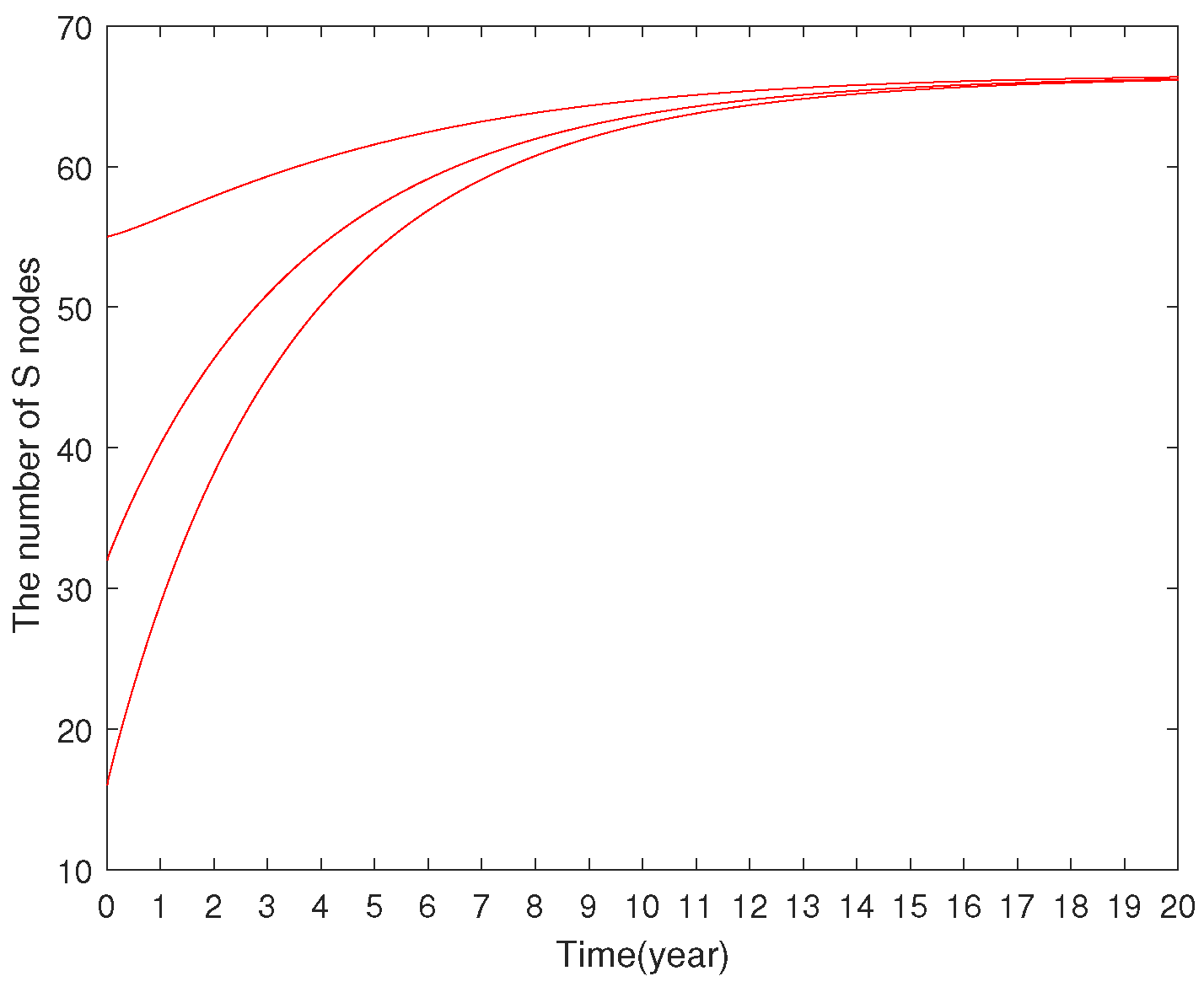
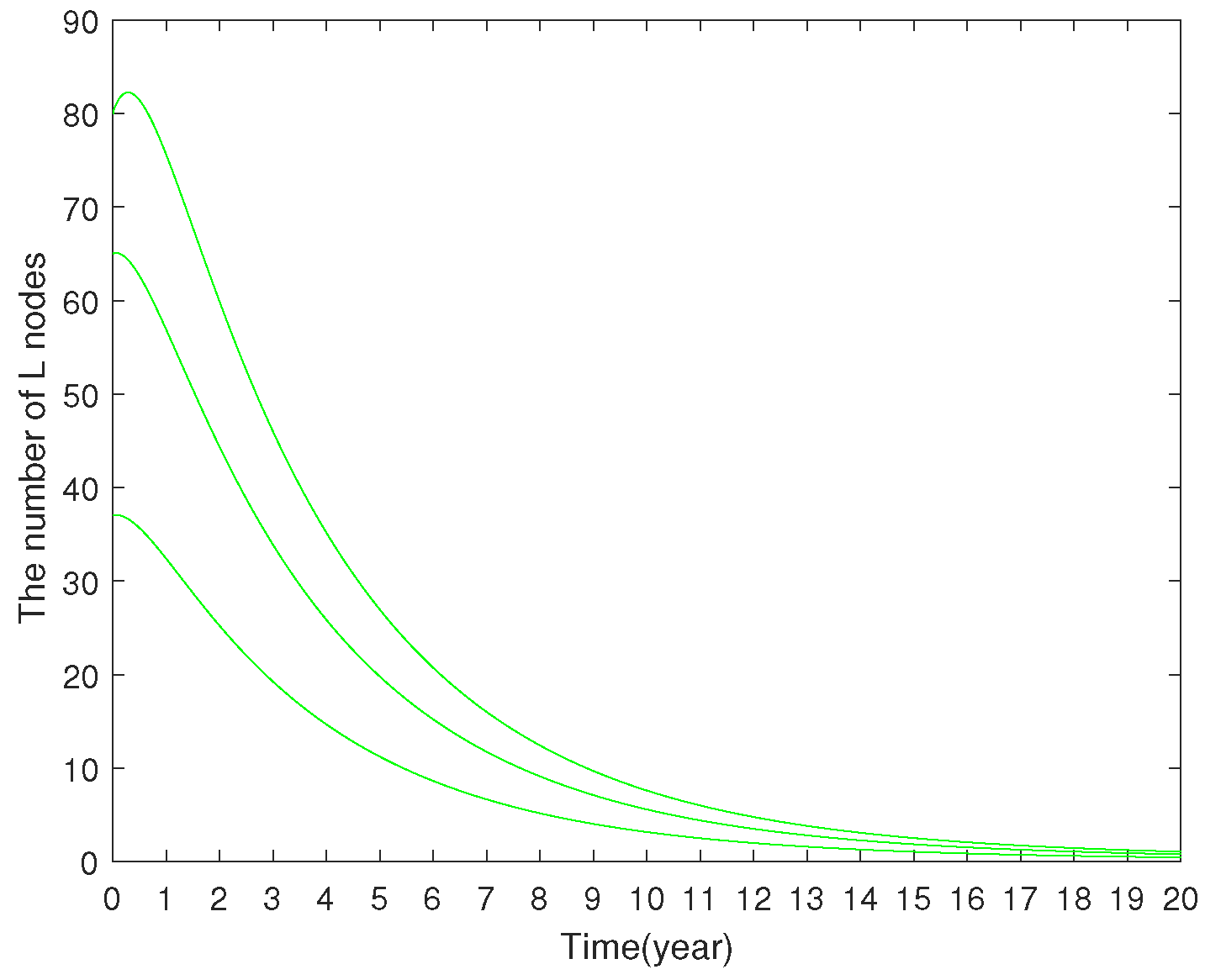
7.1.1. Stability Analysis of Virus-Free Equilibrium

In what follows, we numerically illustrate the analytical results derived in Section 5 through graphical representations. In Figure 1, Figure 2, Figure 3 and Figure 4, we plot the 2D system’s solutions using $a=0.5,b=2,\mu =0.3,\beta =0.003,p=0.5,\gamma =0.002,\alpha =0.9,\epsilon =0.5$ and using three sets of different initial values, which are $\left(S\right(0),L(0),B(0),R(0\left)\right)=(55,80,79,69),\left(S\right(0),L(0),B(0),R(0\left)\right)=(32,65,40,45)$ and $\left(S\right(0),L(0),B(0),R(0\left)\right)=$$(18,47,25,18),$ respectively. For this set of parameter values, ${\mathcal{R}}_0^{\alpha }\approx 0.5473<1$. We demonstrate the comparison of four state functions $S\left(t\right),L\left(t\right),B\left(t\right),R\left(t\right)$ under various initial conditions. As shown in Figure 3, all the curves eventually converge to 0, confirming the stability of the virus-free equilibrium under various initial conditions.

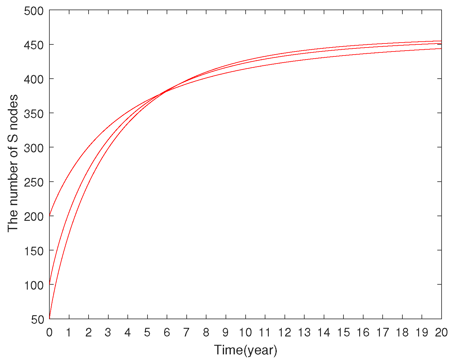
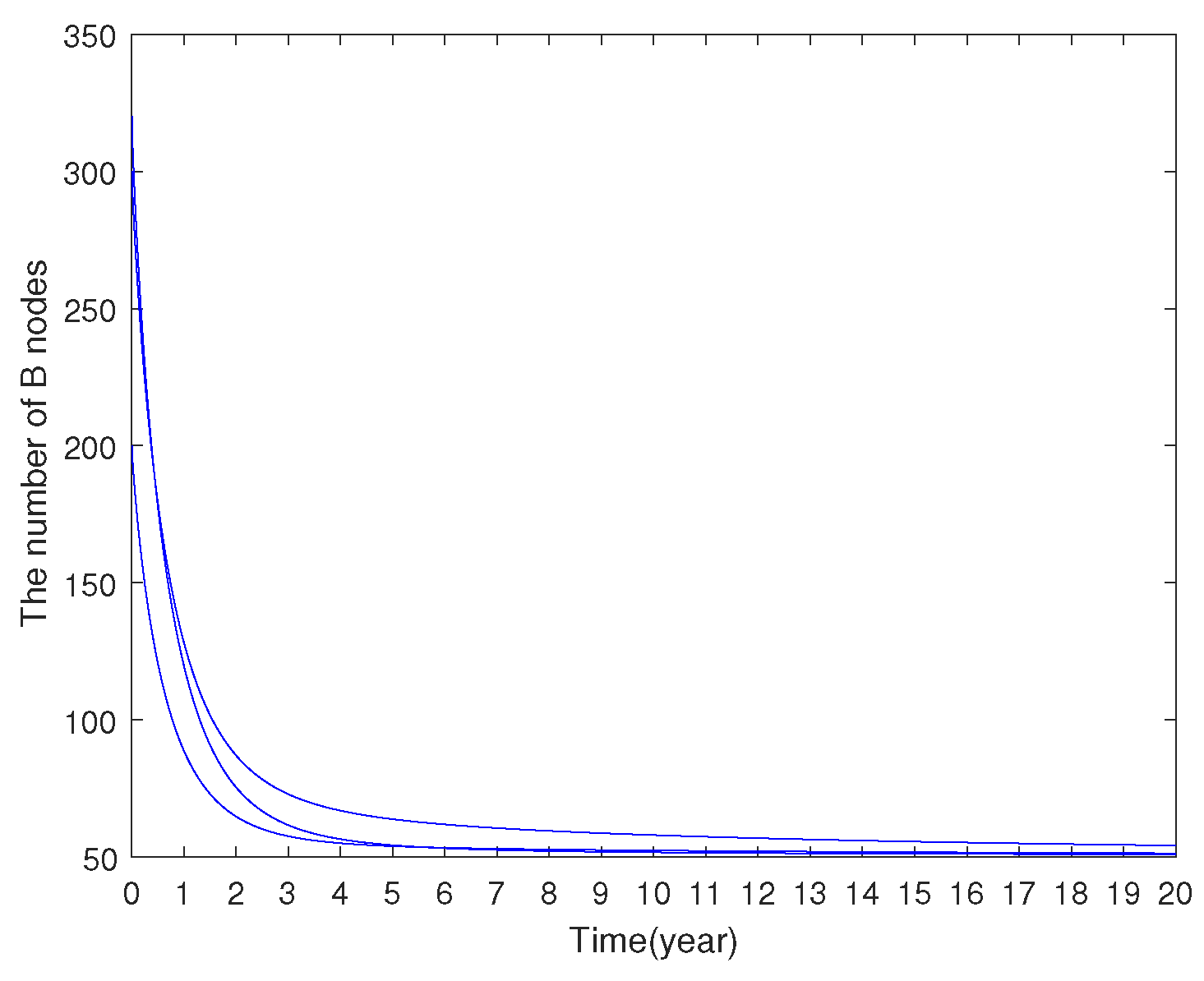
7.1.2. Stability Analysis of Virus-Present Equilibrium

Consider system (3) with $b=0.6,a=0.9,\mu =0.3,\beta =0.3,p=0.5,\gamma =0.002,\alpha =0.9,\epsilon =0.002.$ For this set of parameter values, $(1-p)\gamma =p\epsilon ,$ and ${\mathcal{R}}_0^{\alpha }\approx 1.2483>1$. Here we take three sets of different initial values, which are $\left(S\right(0),L(0),B(0),R(0\left)\right)=(50,300,200,150),\left(S\right(0),L(0),B(0),R(0\left)\right)=(100,425,300,195)$ and $\left(S\right(0),L(0),B(0),R(0\left)\right)$ $=(200,500,310,210),$ respectively. Figure 5 demonstrates that the number of S nodes gradually increases until it reaches a stable level. Figure 6 and Figure 7 demonstrate that the number of L and B nodes gradually diminishes and eventually stabilizes at a certain level. Figure 8 illustrates the progressive increase in the number of R nodes, which eventually stabilizes after reaching a critical threshold. This observation is consistent with Theorem 8.

7.1.3. Model Comparison

In this subsection, we present numerical comparison of several parameters in system (3). First, we show the effect of fractional-order $\alpha$ on the system’s dynamics. Here, we use parameter values given as follows: $b=0.2,a=0.9,\mu =0.3,\beta =0.0002,p=0.5,\gamma =0.002,\epsilon =0.5.$ Figure 9, Figure 10, Figure 11 and Figure 12 show the solution curves of system (3) with initial value $\left(S\right(0),L(0),B(0),R(0\left)\right)=(50,350,550,150),$ when $\alpha =0.90,\alpha =0.93$ and $\alpha =0.5.$ As observed in Figure 9, Figure 10, Figure 11 and Figure 12, the fractional-order $\alpha$ plays a crucial role in influencing the convergence speed of the solutions for system (3).

Next, we investigate the impact of parameter $\mu$ on the system’s dynamics. Here, we choose $b=2,a=0.9,\beta =0.0003,p=0.5,\gamma =0.002,\alpha =0.9,\epsilon =0.5.$ Figure 13, Figure 14, Figure 15 and Figure 16 depict the solution curves of system (3) with initial value $\left(S\right(0),L(0),B(0),R(0\left)\right)=(75,350,550,150),$ when $\mu =0.3,\mu =0.25$ and $\mu =0.2.$ We observe that the higher the probability of the nodes leaving the SCADA system, the faster the number of L and B nodes decrease, which indicates that the nodes leaving the system is conducive to inhibiting the spread of the virus during the virus outbreak.

Finally, we explore the impact of parameter $\beta$ on the system’s dynamics. Here, we assume $b=0.2,a=0.9,\mu =0.3,p=0.5,\gamma =0.002,\alpha =0.9,\epsilon =0.5.$ Figure 17, Figure 18, Figure 19 and Figure 20 describe the solution curves of system (3) with initial value $\left(S\right(0),L(0),B(0),R(0\left)\right)=(50,350,550,150),$ when $\beta =0.002,\beta =0.3$ and $\beta =0.13$. The results show that the smaller the value of $\beta$ is, the easier the virus propagation is inhibited. As is shown in Figure 17, Figure 18, Figure 19 and Figure 20, when $\beta =0.002$, the number of S nodes increase significantly, while the number of L, B and R nodes decrease to varying degrees.

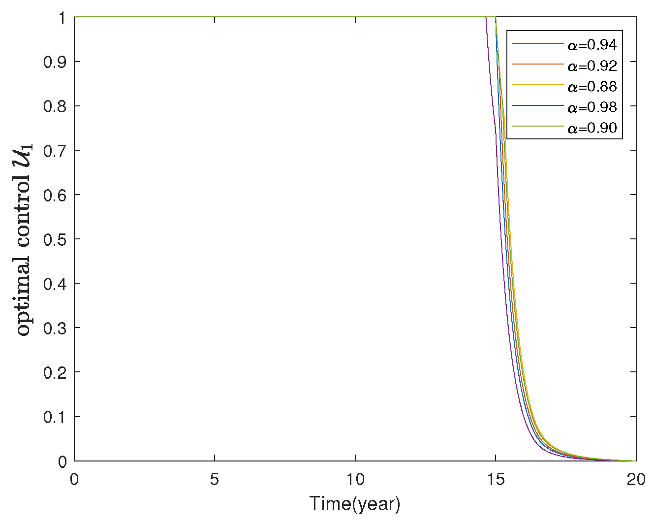
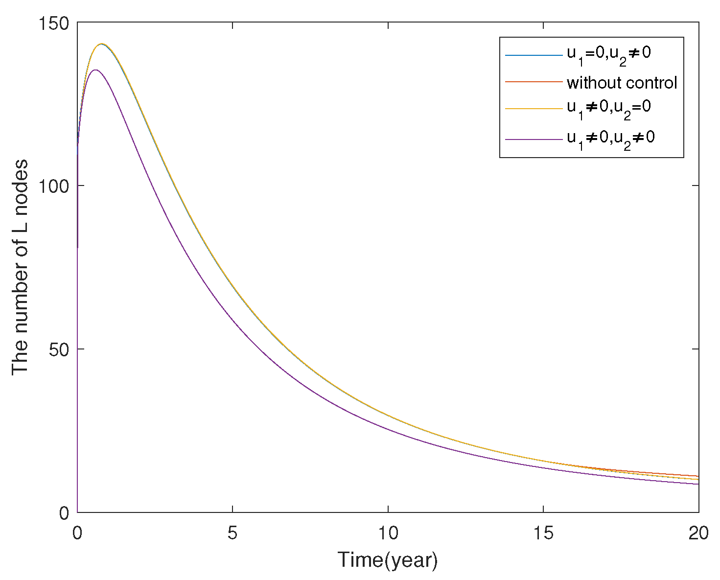
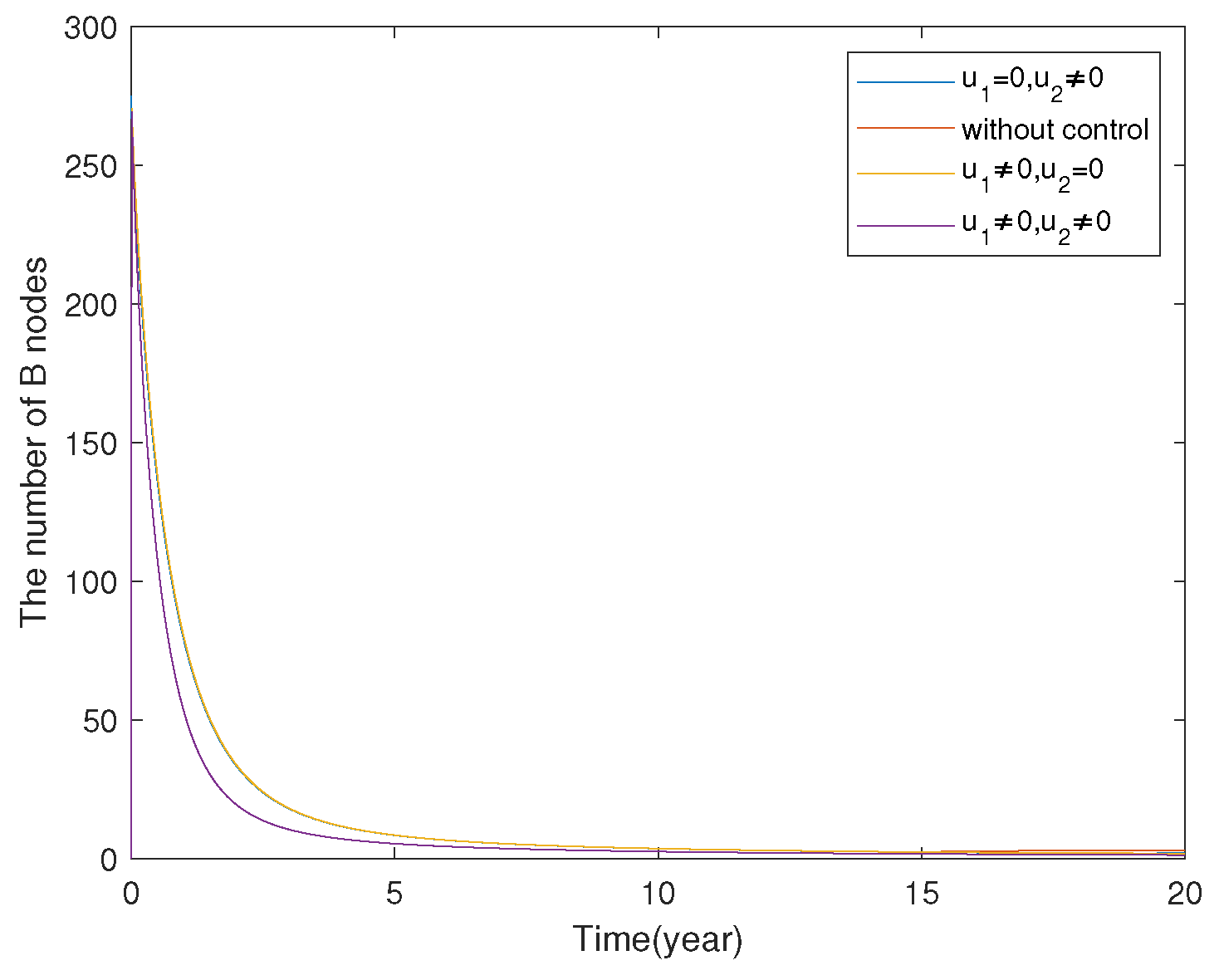
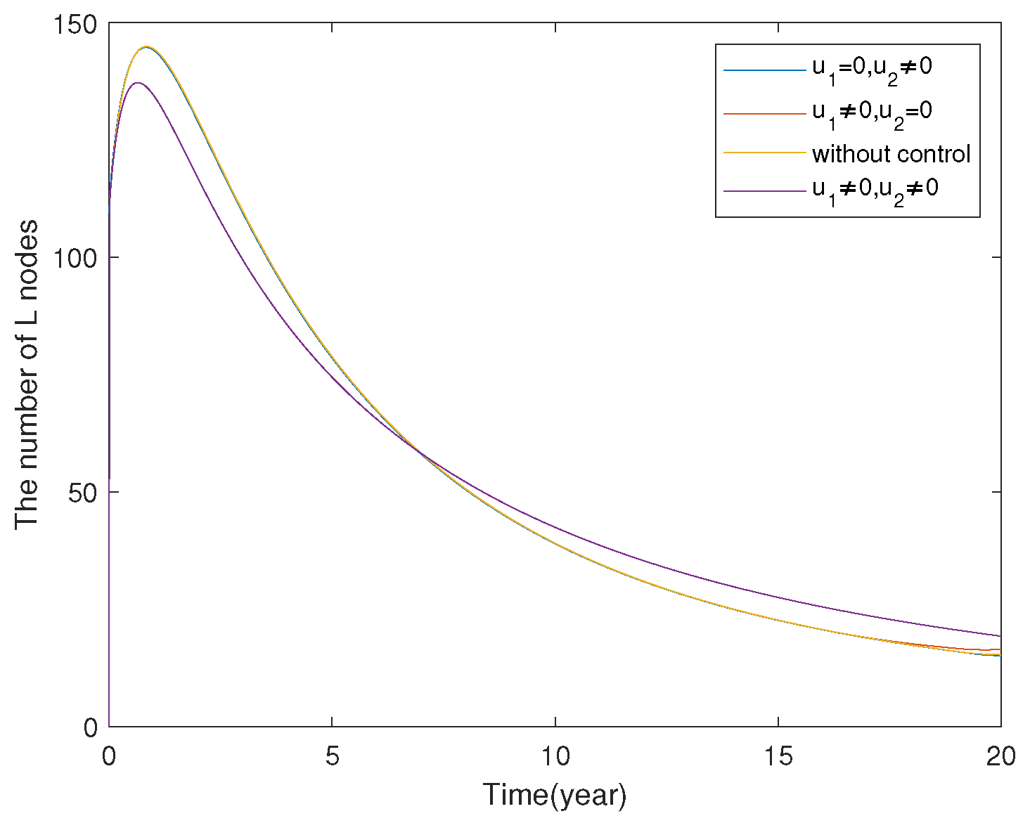
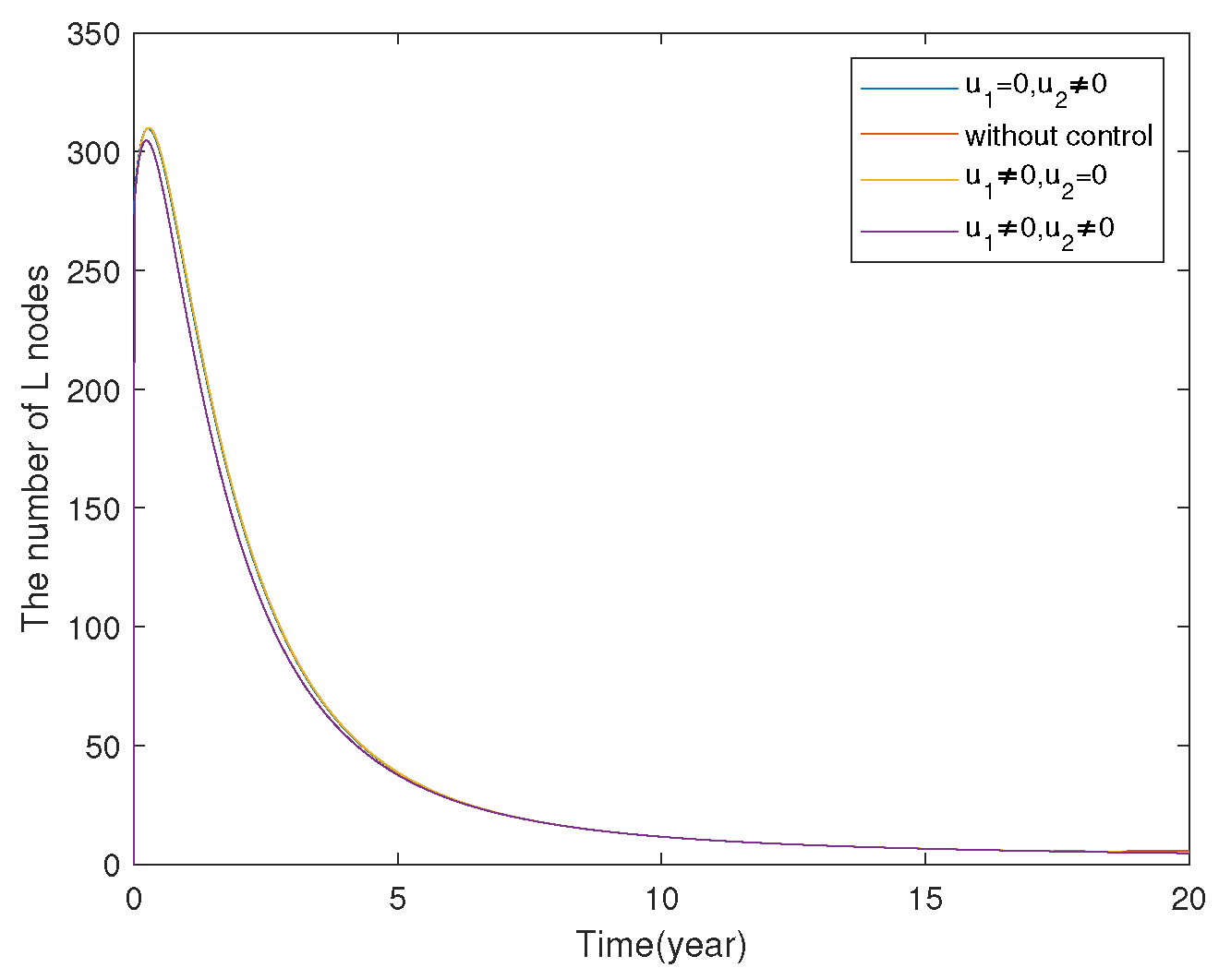
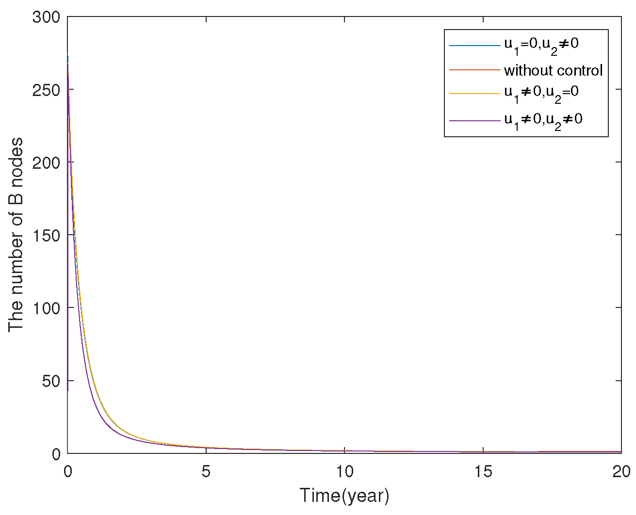
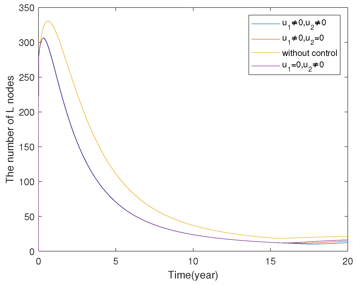
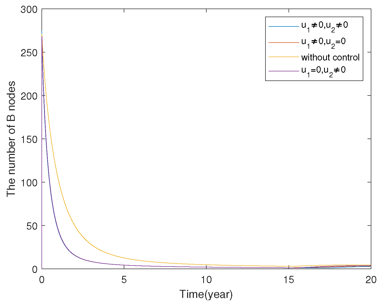
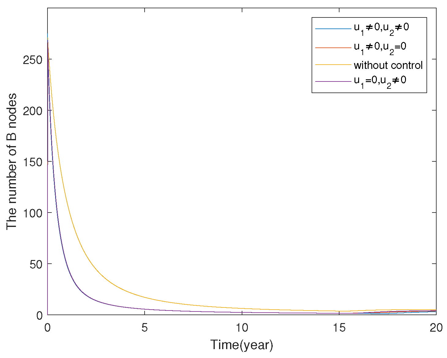
7.2. FOCP of SLBR Transmission

In this subsection, we implement the fractional Euler method in conjunction with the forward-backward predict-evaluate-correct-evaluate approach [49]. To depict the effect of optimal control on the response of the system under study, we set $b=0.5,a=0.5,\mu =0.3,\beta =0.3,p=0.7,\gamma =0.002,\epsilon =0.5,A=100,B_1=0.6$ and $B_2=0.4.$ We assume a final time $T=20$ for optimal control. Figure 21, Figure 22, Figure 23 and Figure 24 show the time series plots of control signals that are applied in the model with initial value $\left(S\right(0),L(0),B(0),R(0\left)\right)=(53,350,325,480),$ when $\alpha =0.94,\alpha =0.92,\alpha =0.88,\alpha =0.98$ and $\alpha =0.90.$ The number of latent, breaking and recovered compartments is reduced in the case where the optimal control scheme is utilized. Figure 25 and Figure 26 show the time series plots of two optimal control strategies $u_1$ and $u_2$ with different fractional-order $\alpha =0.94,\alpha =0.92,\alpha =0.88,\alpha =0.98$ and $\alpha =0.90.$ We observe that the two control measures $u_1$ and $u_2$ should maintain maximum efforts for almost 15 year respectively before decreasing to zero. The order of the derivative can vary across different ranges. When we adjust the order of the derivatives while keeping other parameters constant, the results are very close. This demonstrates that the spread of industrial virus is effectively controlled after raising public safety awareness and optimizing anti-virus software no matter in what range.

Now we study the optimal control results under different infections. We set $b=20,a=0.9,\mu =0.3,p=0.7,\gamma =0.002,\epsilon =0.5$ and $\alpha =0.9.$ We assume a final time $T=20$ for optimal control with initial value $\left(L\right(0),B(0\left)\right)=(110,155)$. We analyze the following cases and compare the associated numerical results.

Strategy 1: Without controls (i.e., $u_1=u_2=0$).

Strategy 2: Using only improvement measures control. The weight coefficients are $A=1000,B_1=1,B_2=0$ (i.e., $u_1\ne 0,u_2=0$).

Strategy 3: Using only treatment measures control. The weight coefficients are $A=1000,B_1=0,B_2=45$ (i.e., $u_1=0,u_2\ne 0$).

Strategy 4: Using all controls. The weight coefficients are $A=1000,B_1=1,B_2=45$. (i.e., $u_1\ne 0,u_2\ne 0$).

Figure 27 and Figure 28 and Figure 29 and Figure 30 show that the number of latent and breaking nodes reduced significantly under Strategy 4 when $\beta =0.0003$ and $\beta =0.003,$ respectively.

We continue to study the optimal control of viruses under different possibilities of virus removal due to anti-virus software. We set $\beta =0.0008$ $b=20,\mu =0.3,p=0.7,\gamma =0.002,\epsilon =0.5$ and $\alpha =0.9.$ We assume a final time $T=20$ for optimal control with initial value $\left(L\right(0),B(0\left)\right)=(280,260)$. We analyze the following cases and compare the associated numerical results.

Strategy 1: Without controls (i.e., $u_1=u_2=0$).

Strategy 2: Using only improvement measures control. The weight coefficients are $A=100,B_1=1,B_2=0$ (i.e., $u_1\ne 0,u_2=0$).

Strategy 3: Using only treatment measures control. The weight coefficients are $A=100,B_1=0,B_2=55$ (i.e., $u_1=0,u_2\ne 0$).

Strategy 4: Using all controls. The weight coefficients are $A=100,B_1=1,B_2=55$. (i.e., $u_1\ne 0,u_2\ne 0$).

Figure 31 and Figure 32 and Figure 33 and Figure 34 show that using two controls at one time is better than using only one control when $a=0.9$ and $a=0.4,$ respectively.

Finally, we study the control under different possibilities of virus outbreak in RTUs with latency. We set $\beta =0.0008$ $b=20,\mu =0.3,p=0.7,a=0.9,\epsilon =0.5$ and $\alpha =0.9.$ We assume a final time $T=20$ for optimal control with initial value $\left(L\right(0),B(0\left)\right)=(270,260)$. We analyze the following cases and compare the associated numerical results.

Strategy 1: Without controls (i.e., $u_1=u_2=0$).

Strategy 2: Using only improvement measures control. The weight coefficients are $A=100,B_1=23,B_2=0$ (i.e., $u_1\ne 0,u_2=0$).

Strategy 3: Using only treatment measures control. The weight coefficients are $A=100,B_1=0,B_2=76$ (i.e., $u_1=0,u_2\ne 0$).

Strategy 4: Using all controls. The weight coefficients are $A=1000,B_1=23,B_2=76$. (i.e., $u_1\ne 0,u_2\ne 0$).

When $\gamma$ is set to 0.004 and 0.09, Figure 35 and Figure 36 and Figure 37 and Figure 38 highlight the significance of the controls $u_1$ and $u_2$, respectively. The presence of these controls rapidly reduces the quantities of L and B nodes.

8. Conclusions

This paper explores a generalized mathematical model for the transmission dynamics of industrial virus based on SCADA system in the form of fractional-order model with a well-known Caputo fractional derivative. Theoretically, we have discussed the well-posedness of the given fractional-order model such as existence and uniqueness of solutions, non-negativity and uniform boundedness as well as stability of the equilibrium points. Moreover, the control parameters of the specified fractional-order model have been treated as time-dependent variables to establish a fractional-order optimal control problem (FOCP) based on the proposed model. Also, conditions for fractional optimal control of industrial virus have been derived and analyzed. Numerical methods and graphical representations are employed to validate the analytical findings. We utilize the ABMPC algorithm to generate images under various control conditions. We have created visualizations to illustrate the effects of final control under varying conditions of some key factors. As a result, we present a comprehensive set of images for optimal control analysis, which enhances confidence in the derived results. It follows from the research results that we should raise public safety awareness and optimize the anti-virus software with the aim of stopping industrial virus infection. Additionally, the method proposed in this study can be readily adapted to address other mathematical models related to the spread of infectious agents such as plant diseases, human infectious diseases and so on.

The actions of industrial viruses are undoubtedly more intricate and varied than what existing mathematical models can fully represent. In practical situations, a computer virus may start propagating the moment an infected file is opened by a user. Similar to infectious diseases in humans, computer viruses often experience an incubation period before showing symptoms or impacting other systems. However, a limitation of current research is the oversight of time delays.

Potential directions for future research include the following:

• Delay in infection: we plan to integrate time delay into the current model. When the anti-virus software is installed, the virus will be cleared. This clearance is modeled as the virus clearance gap delay $\tau$. We will prove the existence and uniqueness of the solution, establish the boundedness of the solution, analyze the stability of the equilibrium points and the occurrence of Hopf bifurcation and, finally, perform numerical simulations to explore the dynamic behavior of the model.
• Backward bifurcation: examines the phenomenon of “reversal” or “backward transition” during the shift from a stable state to an unstable state. In certain situations, computer viruses do not entirely vanish but instead reach a stable endogenous state. Research on backward bifurcation plays a critical role in shaping effective prevention and control strategies.
• Focus on the incidence rate: explore its generalized form. The spread of many viruses demonstrates nonlinear dynamics. By extending the infection rate to a generalized incidence rate, we can more accurately simulate these complex patterns and adapt the model to a broader spectrum of real-world situations.

References

1. Pliatsios, D.; Sarigiannidis, P.; Lagkas, T. A survey on SCADA systems: Secure protocols, incidents, threats, and tractics. IEEE Commun. Surv. Tutor. 2020, 22, 1942–1976. [Google Scholar] [CrossRef]
2. Ajmal, A.B.; Alam, M.; Khaliq, A.A.; Khan, S.; Qadir, Z.; Mahmud, M.A.P. Last line of defence: Reliability through inducing cyber threat hunting with deception in SCADA networks. IEEE Access 2021, 9, 126789–126800. [Google Scholar] [CrossRef]
3. Masood, Z.; Raja, M.A.Z.; Chaudhary, N.I.; Cheema, K.M.; Milyani, A.H. Fractional dynamics of Stuxnet virus propagation in industrial control systems. Mathematics 2021, 9, 2160. [Google Scholar] [CrossRef]
4. Kephart, J.O.; White, S.R. Directed-graph epidemiological models of computer virus. In Proceedings of the 1991 IEEE Computer Society Symposium on Research in Security and Privacy, Oakland, CA, USA, 20–22 May 1991; pp. 343–359. [Google Scholar]
5. Zhu, Q.; Zhang, G.; Luo, X.; Gan, C. An industrial virus-propagation model based on SCADA system. Inform. Sci. 2023, 630, 546–566. [Google Scholar] [CrossRef]
6. Sheng, C.; Yao, Y.; Fu, Q.; Yang, W.; Liu, Y. A cyber-physical model for SCADA system and its intrusion detection. Comput. Netw. 2020, 185, 37. [Google Scholar] [CrossRef]
7. Wu, G.; Zhang, Y.; Zhang, H.; Yu, S.; Shen, S. SIHQR model with time delay for worm spread analysis in IIoT-enabled PLC network 2024. Ad Hoc Netw. 2024, 160, 103504. [Google Scholar] [CrossRef]
8. Thirthar, A.A.; Abboubakar, H.; Alaoui, A.L.; Nisar, K.S. Dynamical behavior of a fractional-order epidemic model for investigating two fear effect functions. Results. Control. Optm 2024, 16, 100474. [Google Scholar] [CrossRef]
9. Avazzadeh, Z.; Nikan, O.; Nguyen, A.T.; Nguyen, V.T. A localized hybrid kernel meshless technique for solving the fractional Rayleigh–Stokes problem for an edge in a viscoelastic fluid. Eng. Anal. Bound. Elem. 2023, 146, 695–705. [Google Scholar] [CrossRef]
10. Murugesan, M.; Santra, S.S.; Jayanathan, L.A.; Baleanu, D. Numerical analysis of fractional order discrete Bloch equations. J. Math. Comput. Sci. 2024, 32, 222–228. [Google Scholar] [CrossRef]
11. Alqahtani, Z.; Almuneef, A.; DarAssi, M.H. Mathematical analysis of fractional Chlamydia pandemic model. Sci. Rep. 2024, 14, 31113. [Google Scholar] [CrossRef]
12. Padisak, J. Seasonal succession of phytoplankton in a large shallow lake(Balaton, Hungary)-a dynamic approach to ecological memory, its possible role and mechanisms. J. Ecol. 1992, 80, 217–230. [Google Scholar] [CrossRef]
13. Podlubny, I. Fractional Differential Equations; Academic Press: New York, NY, USA, 1999. [Google Scholar]
14. Petráš, I. Fractional-Order Nonlinear Systems: Modeling, Analysis and Simulation; Springer: Berlin, Germany; Higher Education Press: Beijing, China, 2011. [Google Scholar]
15. Li, Y.; Chen, Y.; Podlubny, I. Stability of fractional-order nonlinear dynamics systems: Lyapunov direct method and generalized Mittag–Leffler stability. Comput. Math. Appl. 2010, 59, 1810–1821. [Google Scholar] [CrossRef]
16. dos Santos, J.P.C.; Monteiro, E.; Vieira, G.B. Global stability of fractional SIR epidemic model. Proc. Ser. Braz. Soc. Appl. Comput. Math. 2017, 5, 1–7. [Google Scholar]
17. Kheiri, H.; Jafari, M. Optimal control of a fractional-order model for the HIV/AIDS epidemic. Int. J. Biomath. 2018, 6, 1850086. [Google Scholar] [CrossRef]
18. Sadek, L.; Baleanu, D.; Abdo, M.S.; Shatanawi, W. Introducing novel Θ-fractional operators: Advances in fractional calculus. J. King. Saud. Univ. Sci 2024, 36, 103352. [Google Scholar] [CrossRef]
19. Diethelm, K. The Anaysis of Fractional Differential Equations: An Application-Oriented Exposition Using Operators of Caputo Type; Lecture Notes in Mathematics; Springer: Berlin, Germany, 2004. [Google Scholar]
20. Heinz, S.; Ledzewicz, U. Geometric Optimal Control: Theory, Methods and Examples; Springer: Berlin, Germany, 2012. [Google Scholar]
21. You, J.; Li, Y.; Cao, X.; Zhao, D.; Chen, Y.; Zhang, C. Optimal Control of Nonlinear Competitive Epidemic Spreading Processes With Memory in Heterogeneous Networks. IEEE Trans. Netw. Sci. Eng. 2024, 12, 96–109. [Google Scholar] [CrossRef]
22. Ali, H.M.; Pereira, F.L.; Gama, S.M.A. A new approach to the Pontryagin maximum principle for nonlinear fractional optimal control problem. Math. Meth. Appl. Sci. 2016, 39, 3640–3649. [Google Scholar] [CrossRef]
23. Ali, H.M. Necessary Conditions for Constrained Nonsmooth Fractional Optimal Control Problems. Ph.D. Thesis, University of Porto, Porto, Portugal, 2016. [Google Scholar]
24. Ali, H.M.; Ameen, I. Save the pine forests of wilt disease using a fractional optimal control strategy. Chaos Soliton Fract. 2020, 132, 109554. [Google Scholar] [CrossRef]
25. Vellappandi, M.; Kumar, P.; Govindaraj, V.; Albalawi, W. An optimal control problem for mosaic disease via Caputo fractional derivative. Alex. Eng. J. 2022, 61, 8027–8037. [Google Scholar] [CrossRef]
26. Ali, H.M.; Ameen, I. Optimal control strategies of a fractional-order model for Zika virus infection involving various transmissions. Chaos Soliton Fract. 2021, 146, 110864. [Google Scholar] [CrossRef]
27. Sweilam, N.H.; Al-Mekhlafi, S.M.; Albalawi, A.O. Optimal control for a fractional order malaria transmission dynamics mathematical model. Alex. Eng. J. 2020, 59, 1677–1692. [Google Scholar] [CrossRef]
28. Berhe, H.W.; Gebremeskel, A.A.; Melese, Z.T.; Al-arydah, M.T.; Gebremichael, A.A. Modeling and global stability analysis of COVID-19 dynamics with optimal control and cost-effectiveness analysis. Partial. Differ. Equ. Appl. Math. 2024, 11, 100843. [Google Scholar] [CrossRef]
29. Liu, G.; Tan, Z.; Liang, Z.; Chen, H.; Zhong, X. Fractional Optimal Control for Malware Propagation in Internet of Underwater Things. IEEE Internet Things 2024, 11, 11632–11651. [Google Scholar] [CrossRef]
30. La Salle, J.; Lefschetz, S. Stability by Liapunov’s Direct Method; Academic Press: New York, NY, USA, 1961. [Google Scholar]
31. Lyapunov, A.M. The general problem of the stability of motion. Int. J. Control 1992, 55, 531–534. [Google Scholar] [CrossRef]
32. Ameen, I.; Baleanu, D.; Ali, H.M. An efficient algorithm for solving the fractional optimal control of SIRV epidemic model with a combination of vaccination and treatment. Chaos Soliton Fract. 2020, 137, 109892. [Google Scholar] [CrossRef]
33. Ameen, I.; Hidan, M.; Mostefaoui, Z.; Ali, H.M. Fractional optimal control with fish consumption to prevent the risk of coronary heart disease. Complexity 2020, 2020, 9823753. [Google Scholar] [CrossRef]
34. Vargas-De-León, C. Volterra-type Lyapunov functions for fractional-order epidemic systems. Commun. Nonlinear Sci. Numer. Simul. 2015, 24, 75–85. [Google Scholar] [CrossRef]
35. Huo, J.; Zhao, H.; Zhu, L. The effect of vaccines on backward bifurcation in a fractional order HIV model. Nonlinear Anal. Real World Appl. 2015, 26, 289–305. [Google Scholar] [CrossRef]
36. Niu, W.; Fan, M. Control and Research of Computer Virus by Multimedia Technology. Int. J. Inf. Syst. Suppl. 2024, 17, 333896. [Google Scholar] [CrossRef]
37. Diethelm, K. A fractional calculus based model for the simulation of an outbreak of dengue fever. Nonlinear. Dynam 2013, 71, 613–619. [Google Scholar] [CrossRef]
38. Anh Triet, N.; Van Au, V.; Dinh Long, L.; Baleanu, D.; Huy Tuan, N. Regularization of a terminal value problem for time fractional diffusion equation. Math. Method. Appl. Sci. 2020, 43, 3850–3878. [Google Scholar] [CrossRef]
39. Yang, L.; Song, Q.; Liu, Y. Dynamics analysis of a new fractional-order SVEIR-KS model for computer virus propagation: Stability and Hopf bifurcation. Neurocomputing 2024, 598, 128075. [Google Scholar] [CrossRef]
40. Baleanu, D.; Mohammadi, H.; Rezapour, S. A mathematical theoretical study of a particular system of Caputo–Fabrizio fractional differential equations for the Rubella disease model. Adv. Differ. Equ. 2020, 2020, 184. [Google Scholar] [CrossRef]
41. Qureshi, S. Real life application of Caputo fractional derivative for measles epidemiological autonomous dynamical system. Chaos Soliton Fract. 2020, 134, 109744. [Google Scholar] [CrossRef]
42. Ahmed, N.; Wei, Z.; Baleanu, D.; Rafiq, M.; Rehman, M.A. Spatio-temporal numerical modeling of reaction-diffusion measles epidemic system. J. Nonlinear. Sci. 2019, 29, 103101. [Google Scholar] [CrossRef] [PubMed]
43. Odibat, Z.M.; Shawagfeh, N.T. Generalized Taylor’s formula. Appl. Math. Comput. 2007, 186, 286–293. [Google Scholar] [CrossRef]
44. Li, H.; Zhang, L.; Hu, C.; Jiang, Y.; Teng, Z. Dynamical analysis of a fractional-order prey-predator model incorporating a prey refuge. J. Appl. Math. Comput. 2017, 54, 435–439. [Google Scholar] [CrossRef]
45. Driessche, P.V.D.; Watmough, J. Further notes on the basic reproduction number. Math. Epidemiol. 2008, 6, 159–178. [Google Scholar]
46. Lukre, D.L. Differential equations: Classical to controlled. Am. Math. Mon. 1982, 55, 531–534. [Google Scholar]
47. Diethelm, K.; Ford, N.J.; Freed, A.D. A predictor-corrector approach for the numerical solution of fractional differential equations. Nonlinear Dyn. 2002, 29, 3–22. [Google Scholar] [CrossRef]
48. Garrappa, R. On linear stability of predicor-corrector algorithms for fractional differential equations. Int. J. Comput. Math. 2010, 87, 2281–2290. [Google Scholar] [CrossRef]
49. Rosa, S.; Torres, D.F.M. Numerical Fractional Optimal Control of Respiratory Syncytial Virus Infection in Octave/MATLAB. Mathematics 2023, 11, 1511. [Google Scholar] [CrossRef]
Figure 1. Variation of S over time.
Mathematics 13 01338 g001
Figure 2. Variation of L over time.
Mathematics 13 01338 g002
Figure 3. Variation of B over time.
Mathematics 13 01338 g003
Figure 4. Variation of R over time.
Mathematics 13 01338 g004
Figure 5. Variation of S over time.
Mathematics 13 01338 g005
Figure 6. Variation of L over time.
Mathematics 13 01338 g006
Figure 7. Variation of B over time.
Mathematics 13 01338 g007
Figure 8. Variation of R over time.
Mathematics 13 01338 g008
Figure 9. Variation of S over time.
Mathematics 13 01338 g009
Figure 10. Variation of L over time.
Mathematics 13 01338 g010
Figure 11. Variation of B over time.
Mathematics 13 01338 g011
Figure 12. Variation of R over time.
Mathematics 13 01338 g012
Figure 13. Variation of S over time.
Mathematics 13 01338 g013
Figure 14. Variation of L over time.
Mathematics 13 01338 g014
Figure 15. Variation of B over time.
Mathematics 13 01338 g015
Figure 16. Variation of R over time.
Mathematics 13 01338 g016
Figure 17. Variation of S over time.
Mathematics 13 01338 g017
Figure 18. Variation of L over time.
Mathematics 13 01338 g018
Figure 19. Variation of B over time.
Mathematics 13 01338 g019
Figure 20. Variation of R over time.
Mathematics 13 01338 g020
Figure 21. Variation of S over time.
Mathematics 13 01338 g021
Figure 22. Variation of L over time.
Mathematics 13 01338 g022
Figure 23. Variation of B over time.
Mathematics 13 01338 g023
Figure 24. Variation of R over time.
Mathematics 13 01338 g024
Figure 25. Variation of u 1 over time.
Mathematics 13 01338 g025
Figure 26. Variation of u 2 over time.
Mathematics 13 01338 g026
Figure 27. Variation of L over time.
Mathematics 13 01338 g027
Figure 28. Variation of B over time.
Mathematics 13 01338 g028
Figure 29. Variation of L over time.
Mathematics 13 01338 g029
Figure 30. Variation of B over time.
Mathematics 13 01338 g030
Figure 31. Variation of L over time.
Mathematics 13 01338 g031
Figure 32. Variation of B over time.
Mathematics 13 01338 g032
Figure 33. Variation of L over time.
Mathematics 13 01338 g033
Figure 34. Variation of B over time.
Mathematics 13 01338 g034
Figure 35. Variation of L over time.
Mathematics 13 01338 g035
Figure 36. Variation of B over time.
Mathematics 13 01338 g036
Figure 37. Variation of L over time.
Mathematics 13 01338 g037
Figure 38. Variation of B over time.
Mathematics 13 01338 g038
Disclaimer/Publisher’s Note: The statements, opinions and data contained in all publications are solely those of the individual author(s) and contributor(s) and not of MDPI and/or the editor(s). MDPI and/or the editor(s) disclaim responsibility for any injury to people or property resulting from any ideas, methods, instructions or products referred to in the content.