Exploring Consistency in the Three-Option Davidson Model: Bridging Pairwise Comparison Matrices and Stochastic Methods

Abstract

In this paper, data consistency in the three-option Davidson model is investigated. Starting out with the usual consistency definition in pairwise matrices-based methods, we examine its consequences. We formulate an equivalent statement based on the usual PCM-based consistency definition for evaluation results, which aligns with the statement found in the two-option model and establishes a connection between the evaluation results based on PCM and those obtained from the three-option Davidson model. The theoretical results are complemented by findings based on random simulations, through which we also demonstrate the connections: the optimal comparison structures are identical to those in the PCM-based methods and in the two-option Bradley–Terry model.

1. Introduction

Comparisons in pairs is a very useful method for collecting data. It is particularly beneficial in such cases where it is difficult to compare objects to a scale value but it is much easier to determine which is better or worse in relation to each other. Such decisions are much more reliable than the scale values. It is applied in various fields of life: risk analysis [1], psychology [2], decision making in business [3], marketing [4], group decision making [5], architecture [6], sports [7,8,9], politics [10], education [11], environmental studies [12], social sciences [13,14], artificial intelligence [15], and we could continue the list extensively [16,17]. The main goal is rating and ranking the compared objects based on the results of the comparisons. As the primary comparison results are relationships instead of numbers on a scale, the evaluation of paired comparison data requires special evaluation methods.

Two main branches of evaluation methods can be distinguished: the pairwise comparison matrices-based methods (PCMs) and the Thurstone motivated methods (THMMs). An outstanding member of the former family of methods is the Analytic Hierarchy Process (AHP), associated with Saaty’s name [18,19]. The starting point of PCMs is a real squared reciprocal symmetric matrix with dimension $n\times n$, where n is the number of objects to evaluate. Although the decisions between the objects are verbal (equal, better, much better, extremely better, etc.), these decisions are converted into numbers, and these numbers are the elements of the matrices. The conversion methods are different, starting from the usual 1, 3, 5, 7, and 9 elements and the reciprocal numbers to the ratios of the numbers of types of decisions [8]. The evaluation methods are also varied: the most commonly used is the eigenvector method (EM) [20], but the logarithmic least squares method (LLSM) is also frequently applied [21]. The result of the evaluation is a normalized vector with positive coordinates; it is usually called the priority vector. Its coordinates represent the weights (strengths) of the individual objects to be evaluated.

Another branch of the paired comparison models is the stochastic models. In this case, the relations themselves are not converted directly into numbers. Thurstone’s idea that latent probabilistic variables underlie the objects to be evaluated and that decisions depend on the current values of these probabilistic variables holds great potential. Thurstone dealt with the Gauss distribution allowing two options [22], and applied the least squares parameter estimation method. Later, logistic distribution was applied with maximum likelihood estimation (MLE) [23]. The number of options has been extended to three, allowing option ‘equal’ next to options ‘worse’, and ‘better’ [24,25]. More than 3 options were analyzed in [26], applying the least squares estimation method, and in [27], applying MLE and allowing a wide class of distributions.

It is always an exciting challenge in research to recognize the connections between models based on different foundations. In the area of research in the field of comparisons in pairs, it is an interesting question what the relationship between PCMs and stochastic paired comparison methods can be. Based on empirical evidence, a connection was presented between them in the publication [28]. Recently, a theoretical relationship was proved for the two-option Bradley–Terry model and PCM-based methods [29]. The key of the relation was the concept of consistency, i.e., the absence of contradiction among the data [19]. It has been proved that in the case of data consistency, the two-option Bradley–Terry model with MLE parameter estimation and PCMs with LLSM or eigenvector methods provide the same priority vectors. If data are inconsistent, then the optimal comparison structures are proved to be the same structures in the case of 4, 5, and 6 objects to evaluate. However, the relation between the three-option stochastic models and the PCM-based models has not been revealed. This gap is filled in the current paper in the case of a three-option stochastic model.

In this paper, we investigate a stochastic three-option model from the aspects of data consistency. This model is a modified version of the three-option Bradley–Terry model. The modification was performed by Davidson in [30] in order for Luce’s choice axiom to be satisfied in the stochastic model even in the case of three options. In the case of the Bradley–Terry model that allows two options (BT2), Luce’s choice axiom is satisfied. Luce’s choice axiom expresses that the probabilities of the comparison results between two objects depend only on their strengths and are not affected by other objects [31,32], but in the case of the Bradley–Terry model allowing three options in choices (BT3), it is not. However, in Davidson’s modified model, Luce’s choice axiom holds.

Our article is structured as follows. In Section 2, the investigated Davidson model is presented. In Section 3, the concept of consistency in PCM models and the concept of consistency in the Davidson model is detailed, along with their relationship, based on the theoretical considerations. The connection between the Davidson model and PCM-based models is also supported by the simulation results in Section 4. The methodology of the simulation is described in Section 4.1, and in Section 4.2 and Section 4.3, the results of the simulations are presented. Finally, the paper is closed with a brief summary.

2. The Investigated Model: Davidson Model

To ensure that Luce’s choice axiom is satisfied in the model, Davidson introduced a modified three-option model as follows [30].

Consider a vector $\underline{\pi }=({\pi }_1,\dots ,{\pi }_n)$, $0<{\pi }_i$ that satisfies ${\sum }_{i=1}^n{\pi }_i=1$. The probabilities of the options ‘worse’, ‘equal’, and ‘better’ are assumed to be

$$p_{i,j,1}=P\left(i\mathrm{is}‘\mathrm{worse}’\mathrm{than}j\right)={\displaystyle \frac{{\pi }_j}{{\pi }_i+{\pi }_j+\nu \sqrt{{\pi }_i{\pi }_j}}},$$

(1)

$$p_{i,j,2}=P\left(i\mathrm{is}‘\mathrm{equal}’\mathrm{to}j\right)={\displaystyle \frac{\nu \sqrt{{\pi }_i{\pi }_j}}{{\pi }_i+{\pi }_j+\nu \sqrt{{\pi }_i{\pi }_j}}},$$

(2)

$$p_{i,j,3}=P\left(i\mathrm{is}‘\mathrm{better}’\mathrm{than}j\right)={\displaystyle \frac{{\pi }_i}{{\pi }_i+{\pi }_j+\nu \sqrt{{\pi }_i{\pi }_j}}}$$

(3)

with some

$$0<\nu .$$

(4)

It is easy to see that if $\nu =0$, we return to BT2.

One can check, that, due to (1)–(3),

$${\displaystyle \frac{p_{i,j,2}}{\sqrt{p_{i,j,1}·p_{i,j,3}}}}=\nu .$$

(5)

In this model, the Luce’s choice axiom [31,32] is fulfilled as

$${\displaystyle \frac{p_{i,j,3}}{p_{i,j,1}}}={\displaystyle \frac{{\pi }_i}{{\pi }_j}}.$$

(6)

Data are contained in a three-dimensional matrix A. Its element $A_{i,j,k}$ represents the number of decisions according to the comparison of object i and object j, and the result of the decision belongs to option k ($k=1$ stands for ‘worse’, $k=2$ stands for ‘equal’ and $k=3$ stands for option ‘better’). Of course, $A_{i,i,k}=0$ and $k=1,2,3$, and due to the symmetry, $A_{j,i,1}=A_{i,j,3}$ and $A_{j,i,2}=A_{i,j,2}$.

The likelihood function represents the probability of the data as a function of unknown parameters. Assuming an independent sample, it can be written as follows:

$$L\left(A\right|({\pi }_1,\dots ,{\pi }_n,\nu ))=\prod _{k=1}^3\prod _{i=1}^{n-1}\prod _{j=i+1}^n{\left(p_{i,j,k}\right)}^{A_{i,j,k}}.$$

(7)

The log-likelihood function is its logarithm

$$logL\left(A\right|({\pi }_1,\dots ,{\pi }_n,\nu ))=\sum _{k=1}^3\sum _{i=1}^{n-1}\sum _{j=i+1}^n{A}_{i,j,k}·log\left(p_{i,j,k}\right)=\sum _{k=1}^3\sum _{i=1}^n\sum _{j=1;j\ne i}^{n}0.5·(A_{i,j,k}·log\left(p_{i,j,k}\right)).$$

(8)

The maximum likelihood estimation of the parameters (MLEP) is the argument of the maximum value of the function (8), i.e.,

$$\widehat{B}=(\widehat{\underline{\pi }},\widehat{\nu })=\underset{\underline{\pi }>0,\nu >0,{\sum }_{i=1}^n{\pi }_i=1}{argmax}logL\left(A\right|({\pi }_1,\dots ,{\pi }_n,\nu )).$$

(9)

Note that the parameters ${\pi }_i$ can be multiplied by a positive constant without changing (8). This multiplication possibility is eliminated by requiring that the sum of the coordinates equals 1. Moreover, if all data $A_{i,j,k}$ are multiplied by the same positive constant, the maximum value would also be multiplied by it, but the argument of the maximum value, i.e., the estimate MLEP, would not change.

To investigate the evaluability of the data, i.e., the existence of the maximum value and the uniqueness of its argument, we need the following graph definitions and theorem.

Definition 1

(graph of comparisons $GR{C}_E^{\left(3\right)}$). Let the objects to be evaluated be assigned the nodes of the graph. Let there be an edge between i and j ($i-j$) if there is a comparison between i and j, i.e.,

$$\sum _{k=1}^3{A}_{i,j,k}>0.$$

(10)

Let the set of edges be denoted by E. This graph is denoted by $GR{C}_E^{\left(3\right)}$.

Definition 2

(directed graph $GRDI{R}_A^{\left(3\right)}$). Let the objects to be evaluated be assigned the nodes of the graph. Let there be a directed edge from i to j (i → j) if there is a decision that i is considered to be ’better’ than j, that is, $A_{i,j,3}>0$. Let there be bi-directed edges from i to j ($i⟷j$) if i is considered equal to j according to a decision, that is $A_{i,j,2}>0$. This graph is denoted by $GRDI{R}_A^{\left(3\right)}$.

Theorem 1

([33]). The maximum value of the log-likelihood function (8) exists and the argument is unique under the conditions $0<\underline{\pi },$$0<\nu$ and ${\sum }_{i=1}^n{\pi }_i=1$, if and only if data matrix A satisfies the following set of conditions:

(A) 

There is at least one index pair $(i,j)$ for which $0<A_{i,j,2}$.

(B) 

For any partition S and $\overline{S}$, $S\cup \overline{S}=\{1,2,\dots ,n\}$, $S\cap \overline{S}=\varnothing$, there is at least one element $i\in S$ and $j\in \overline{S}$, for which $0<A_{i,j,2}$, or there are two (not necessarily different) pairs $(i_1,j_1)\mathrm{and}(i_2,j_2)$, $i_1,i_2\in S$, $j_1,j_2\in \overline{S}$, for which $0<A_{i_1,j_1,3}$ and $0<A_{i_2,j_2,1}$.

(C) 

With the graph definition given in Definition 2, there exists such a directed cycle $(i_1,i_2,i_3,\dots ,i_l,i_1)$, where $i_k,k=1,2,\dots ,l$ are nodes, in which the number of the directed ’better’ edges exceeds the number of the bi-directed ‘equal’ edges.

The proof of Theorem 1 can be found in [33].

3. Consistency and Its Theoretical Consequences

3.1. Consistency of Data in the Case of PCM-Based Methods

The concept of consistency and the degree of data inconsistency are central issues in PCMs. The most commonly used concept of consistency is the following: denote by $a_{i,j}$$(i=1,\dots ,n$, $j=1,\dots ,n)$ the elements of the (multiplicative) pairwise comparison matrix $\mathit{a}$, $a_{i,j}={\displaystyle \frac{1}{a_{j,i}}}$. If the comparison is complete, (every object is compared to any other object, i.e., $0<a_{i,j},$ $i=1,\dots ,n$, $j=1,\dots ,n$), then consistency means the following relations:

$$a_{i,j}=a_{i,l}·a_{l,j}\forall i=1,\dots ,n;j=1,\dots ,n,l=1,\dots ,n.$$

(11)

In the case of incomplete comparisons, in matrix $\mathit{a}$, the elements corresponding to the missing comparisons will remain empty. In such cases, the following generalized consistency definition is given [34]. For all cycles ($i_1,\dots ,i_l,i_1$) in the graph of comparisons, the following equality holds:

$$a_{i_1,i_2}·a_{i_2,i_3}·\cdots ·a_{i_l,i_1}=1.$$

(12)

Even in complete and incomplete cases, assuming a consistent data matrix $\mathit{a}$, the result of the evaluation is a priority vector $\underline{w}=(w_1,\dots ,w_n)$, with properties $0<w_i,i=1,\dots ,n$, and ${\sum }_i^n{w}_i=1$, then

$$a_{i,j}={\displaystyle \frac{w_i}{w_j}},$$

(13)

and relation (13) guarantees the consistency.

Numerous metrics have been developed to measure inconsistency [18,35,36]. Recently, the case of incomplete comparisons has become the subject of research; see, for example, [37].

3.2. Consistency in Davidson Model

The concept of consistency is rarely examined in the case of the models with a stochastic background. In the publication [29], the two-option Bradley–Terry model was scrutinized, and the consistency of the data was defined within it. In the conference paper [38], the three-option Davidson model was investigated, and now these examinations will be extended.

First, we prove that if we start with a parameter set and we define data as the probabilities given by (1)–(3), moreover, the graph of comparisons $GR{C}_E^{\left(3\right)}$ is connected, then the maximum likelihood estimation of the parameters coincides with the starting parameter set.

Theorem 2.

Let ${\underline{\pi }}^{\left(0\right)}=({\pi }_1^{\left(0\right)},\dots ,{\pi }_n^{\left(0\right)})$ be a starting initial vector with $0<{\pi }_i^{\left(0\right)}$ and ${\sum }_{i=1}^n{\pi }_i^{\left(0\right)}=1$, and $0<{\nu }^{\left(0\right)}$. Let $p_{i,j,k}^{\left(0\right)}$ be computed from this parameter set $({\underline{\pi }}^{\left(0\right)},{\nu }^{\left(0\right)})$ applying formulas (1), (2), and (3). Fix a graph of comparisons, incomplete or complete $GR{C}_E^{\left(3\right)}$, the set of its edges is denoted by E. Let the data be defined as follows:

$$A_{i,j,k}^{\left(0\right)}=\left\{\begin{array}{c}{p}_{i,j,k}^{\left(0\right)},\mathit{if}(i,j)\in E\\ 0,\mathit{otherwise}\end{array}\right.$$

(14)

If the graph of comparisons $GR{C}_E^{\left(3\right)}$ is connected, then the log-likelihood function (8) attains its maximum value at ${\underline{\pi }}^{\left(0\right)}=({\pi }_1^{\left(0\right)},\dots ,{\pi }_n^{\left(0\right)})$, and ${\nu }^{\left(0\right)}$, i.e.,

$$(\underline{\widehat{\pi }},\widehat{\nu })=({\underline{\pi }}^{\left(0\right)},{\nu }^{\left(0\right)}).$$

(15)

Proof. 

First of all, we note that if $(i,j)\in E$, then $0<p_{i,j,1}^{\left(0\right)}$, $0<p_{i,j,2}^{\left(0\right)}$, and $0<p_{i,j,3}^{\left(0\right)}$. In other words, for a fixed pair $(i,j)$, all data $A_{i,j,k}^{\left(0\right)}$ for $k=1,2,3$ are positive, or all data $A_{i,j,k}^{\left(0\right)}$ for $k=1,2,3$ are equal to zero. Therefore, the connection of the comparison graph $GR{C}_E^{\left(3\right)}$ belonging to the data set $A^{\left(0\right)}$ guarantees that conditions (A), (B), and (C) are satisfied. Consequently, if the data are defined by (14), the necessary and sufficient condition for a unique maximizer is the connectedness of the graph $GR{C}_E^{\left(3\right)}$.

Let us define the following function:

$$\begin{array}{c}\hfill F(x_{1,1},x_{1,2},\dots ,x_{s,1},x_{s,2})=\sum _{s=1}^{\left|E\right|}{B}_{s,1}·log\left(x_{s,1}\right)+B_{s,2}·log\left(x_{s,2}\right)+\\ \hfill +B_{s,3}·log((1-x_{s,1}-x_{s,2}),\end{array}$$

(16)

for the regions $0<x_{s,1}$, $0<x_{s,2}$ and $x_{s,1}+x_{s,2}<1.$ Here, $\left|E\right|$ is the number of compared pairs, and there is a one-to-one correspondence between the indices s and the elements of the set of vertices $(i,j)$ in E. Moreover, in the log-likelihood function (8), $B_{s,k}=A_{i,j,k}^{\left(0\right)}$, $x_{s,1}=p_{i,j,1}$ and $x_{s,2}=p_{i,j,2}$. To find the maximum value, take the partial derivative with respect to $x_{s,1}$ and $x_{s,2}$, $s=1,\dots ,\left|E\right|$, and we obtain

$$B_{s,1}·{\displaystyle \frac{1}{x_{s,1}}}-B_{s,3}·{\displaystyle \frac{1}{1-x_{s,1}-x_{s,2}}}=0.$$

(17)

and

$$B_{s,2}·{\displaystyle \frac{1}{x_{s,2}}}-B_{s,3}·{\displaystyle \frac{1}{1-x_{s,1}-x_{s,2}}}=0.$$

(18)

From (17) and (18), it follows that

$$x_{s,1}=B_{s,1}\mathrm{and}{x}_{s,2}=B_{s,2}.$$

(19)

Using the Hesse matrix, we can check that at this point, the extreme value exists, and it is the maximum.

Now the question is whether there exists such a parameter set ($\widehat{\underline{\pi }},\widehat{\nu }$) for which

$$x_{s,1}={\displaystyle \frac{{\widehat{\pi }}_j}{{\widehat{\pi }}_i+{\widehat{\pi }}_j+\widehat{\nu }\sqrt{{\widehat{\pi }}_i{\widehat{\pi }}_j}}}$$

(20)

and

$$x_{s,2}={\displaystyle \frac{\widehat{\nu }\sqrt{{\widehat{\pi }}_i·{\widehat{\pi }}_j}}{{\widehat{\pi }}_i+{\widehat{\pi }}_j+\widehat{\nu }\sqrt{{\widehat{\pi }}_i·{\widehat{\pi }}_j}}}.$$

(21)

We know that the starting parameter set (${\underline{\pi }}^{\left(0\right)},{\nu }^{\left(0\right)}$) satisfies Equations (20) and (21). Moreover, as the argument of the maximum value is unique, we can conclude that

$$(\underline{\widehat{\pi }},\widehat{\nu })=({\underline{\pi }}^{\left(0\right)},{\nu }^{\left(0\right)}).$$

(22)

□

Now, we will show that the priority vectors obtained using the LLSM and EM methods with PCM match the evaluation results obtained in the Davidson model if the elements of the PC matrix are defined based on the probabilities from the previous statement.

Theorem 3.

Let us define the data by (14), and let the elements of the PCM $\mathit{a}$ be

$$a_{i,j}={\displaystyle \frac{A_{i,j,3}^{\left(0\right)}}{A_{i,j,1}^{\left(0\right)}}}={\displaystyle \frac{P({\xi }_j<{\xi }_i)}{P({\xi }_i<{\xi }_j)}}={\displaystyle \frac{{\pi }_i^{\left(0\right)}}{{\pi }_j^{\left(0\right)}}},\mathit{if}(i,j)\in E.$$

(23)

Assume that the graph of comparison $GR{C}_E^{\left(3\right)}$ is connected. Then, the results of the evaluation of PCM $\mathit{a}$ by LLSM and also by EM coincide with the MLEP in the Davidson model, i.e., ${\underline{\pi }}^{\left(0\right)}$.

Proof. 

Due to the definition of $a_{i,j}$, the PCM is consistent; therefore, if the result of the evaluation is ${\underline{w}}^{\left(0\right)}$, then $a_{i,j}={\displaystyle \frac{w_i^{\left(0\right)}}{w_j^{\left(0\right)}}}$. This property holds for ${\underline{\pi }}^{\left(0\right)}$. As the sums of the coordinates equal 1 in both cases, the equality of the vectors is guaranteed. □

The following statement expresses the equivalence between the concept of consistency used for PCMs (see (12)) and the data ratio written as the ratio of the coordinates of the priority vector in the Davidson model.

Theorem 4.

Let $E=\{(i,j):0<{\sum }_{k=1}^3{A}_{i,j,k}\}$ and $GR{C}_E^{\left(3\right)}$ be the graph of comparisons defined by the edges in E. Suppose that $GR{C}_E^{\left(3\right)}$ is connected. Assume that the data $A_{i,j,k}$ satisfy the following requirements.

If $(i,j)\in E$, then

$$0<A_{i,j,k},k=1,2,3,$$

(24)

and moreover,

$$A_{i,j,2}=\nu ·\sqrt{A_{i,j,1}·A_{i,j,3}}$$

(25)

with a common value $0<\nu$. Let us introduce the notation

$$h_{i,j}={\displaystyle \frac{A_{i,j,3}}{A_{i,j,1}}}.$$

(26)

For every cycle $(i_1,i_2,\dots ,i_l,i_1)\in GR{C}_E^{\left(3\right)}$

$$h_{i_1,i_2}·\cdots ·h_{i_l,i_1}=1$$

(27)

holds if and only if

$${\displaystyle \frac{A_{i,j,3}}{A_{i,j,1}}}={\displaystyle \frac{{\widehat{\pi }}_i}{{\widehat{\pi }}_j}}.$$

(28)

for the MLEP $\underline{\widehat{\pi }}$ in (9), with coordinates $0<{\widehat{\pi }}_i$ and ${\sum }_{i=1}^n{\widehat{\pi }}_i=1$.

Proof. 

First, we prove that (27) implies (28).

The log-likelihood function (16) with $B_{s,k}$=$A_{i,j,k}$ and $x_{s,k}=p_{i,j,k}$ takes its extreme value at

$$x_{s,1}={\displaystyle \frac{B_{s,1}}{B_{s,1}+B_{s,2}+B_{s,3}}}={\displaystyle \frac{A_{i,j,1}}{A_{i,j,1}+A_{i,j,2}+A_{i,j,3}}}$$

(29)

and

$$x_{s,3}={\displaystyle \frac{B_{s,3}}{B_{s,1}+B_{s,2}+B_{s,3}}}={\displaystyle \frac{A_{i,j,3}}{A_{i,j,1}+A_{i,j,2}+A_{i,j,3}}}.$$

(30)

It can be checked that the extreme value at this point is the maximum. We verify whether there exists such a vector $\underline{\widehat{\pi }}$, $0<{\widehat{\pi }}_i$, ${\sum }_{i=1}^n{\widehat{\pi }}_i=1$, and $0<\widehat{\nu }$,

$${\displaystyle \frac{A_{i,j,1}}{A_{i,j,1}+A_{i,j,2}+A_{i,j,3}}}={\displaystyle \frac{{\widehat{\pi }}_j}{{\widehat{\pi }}_i+{\widehat{\pi }}_j+\widehat{\nu }\sqrt{{\widehat{\pi }}_i·{\widehat{\pi }}_j}}},$$

(31)

$${\displaystyle \frac{A_{i,j,2}}{A_{i,j,1}+A_{i,j,2}+A_{i,j,3}}}={\displaystyle \frac{\widehat{\nu }\sqrt{\widehat{{\pi }_i}·\widehat{{\pi }_j}}}{{\widehat{\pi }}_i+{\widehat{\pi }}_j+\widehat{\nu }\sqrt{{\widehat{\pi }}_i·{\widehat{\pi }}_j}}},$$

(32)

$${\displaystyle \frac{A_{i,j,3}}{A_{i,j,1}+A_{i,j,2}+A_{i,j,3}}}={\displaystyle \frac{{\widehat{\pi }}_j}{{\widehat{\pi }}_i+{\widehat{\pi }}_j+\widehat{\nu }\sqrt{{\widehat{\pi }}_i·{\widehat{\pi }}_j}}}.$$

(33)

To satisfy the equalities (31)–(33), the equalities

$${\displaystyle \frac{A_{i,j,3}}{A_{i,j,1}}}={\displaystyle \frac{{\widehat{\pi }}_i}{{\widehat{\pi }}_j}}$$

(34)

and

$$\widehat{\nu }={\displaystyle \frac{A_{i,j,2}}{\sqrt{A_{i,j,1}·A_{i,j,3}}}}$$

(35)

have to be satisfied for every $(i,j)\in E$. (35) is satisfied due to (25), that is, $\widehat{\nu }=\nu$ in (35).

Let us turn to (34). If $GR{C}_E^{\left(3\right)}$ is a spanning tree, then start from object 1, and suppose that ${\widehat{\pi }}_1^1=1$. Now, walking along the edges in $GR{C}_E^{\left(3\right)}$, the coordinate of ${\underline{\widehat{\pi }}}^1$ can be defined by

$${\widehat{\pi }}_j^1={\widehat{\pi }}_i^1·{\displaystyle \frac{A_{i,j,1}}{A_{i,j,3}}}.$$

(36)

There is no cycle in a spanning tree, therefore, every coordinate is reached once and only once. Taking

$${\widehat{\pi }}_i={\displaystyle \frac{{\widehat{\pi }}_i^1}{{\sum }_{k=1}^n{\widehat{\pi }}_k^1}}$$

(37)

we obtain an appropriate vector in the case of a spanning tree.

Turn to the case where $GR{C}_E^{\left(3\right)}$ is not a spanning tree. Take an edge $(i,j)\in E$. Let I be a spanning tree in $GR{C}_E^{\left(3\right)}$, $I\subset GR{C}_E^{\left(3\right)}$. Define the parameter vector as in the case of spanning trees. If $(i,j)$ is an edge in the tree I, then (34) holds. If $(i,j)$ is not contained among the edges of I, then there exists a path from i to j in the spanning tree $GR{C}_I^{\left(3\right)}$; let it be ($i=i_1,i_2,\dots ,i_l=j)$. Consider the cycle $(i_1,i_2,\dots ,i_l,i_1)$. As (27) holds, and

$${\displaystyle \frac{A_{i_1,i_2,3}}{A_{i_1,i_2,1}}}={\displaystyle \frac{{\widehat{\pi }}_{i_1}}{{\widehat{\pi }}_{i_2}}}$$

(38)

and so on, we can conclude that

$${\displaystyle \frac{{\widehat{\pi }}_{i_1}}{{\widehat{\pi }}_{i_l}}}·h_{i_l,i_1}=1$$

(39)

i.e.,

$$h_{j,i}={\displaystyle \frac{{\widehat{\pi }}_j}{{\widehat{\pi }}_i}}.$$

(40)

So, one can see that (34) is true for every edge in $GR{C}_E^{\left(3\right)}$.

Now, let us consider the opposite direction of the equivalence. If (28) holds, then multiply these values in the case of the edges in a cycle. After performing the simplifications, it is obvious that the product would be 1. □

Remark 1.

We draw attention to the fact that, if the graph of comparisons is connected and the data satisfy (24) and (25), as a consequence of (27), we obtain that the data are proportional to the probabilities

$$A_{i,j,1}=K_{i,j}·{\displaystyle \frac{{\widehat{\pi }}_j}{{\widehat{\pi }}_i+{\widehat{\pi }}_j+\widehat{\nu }\sqrt{{\widehat{\pi }}_i·{\widehat{\pi }}_j}}},$$

(41)

$$A_{i,j,2}=K_{i,j}·{\displaystyle \frac{\widehat{\nu }\sqrt{\widehat{{\pi }_i}·\widehat{{\pi }_j}}}{{\widehat{\pi }}_i+{\widehat{\pi }}_j+\widehat{\nu }\sqrt{{\widehat{\pi }}_i·{\widehat{\pi }}_j}}},$$

(42)

$$A_{i,j,3}=K_{i,j}·{\displaystyle \frac{{\widehat{\pi }}_i}{{\widehat{\pi }}_i+{\widehat{\pi }}_j+\widehat{\nu }\sqrt{{\widehat{\pi }}_i·{\widehat{\pi }}_j}}}.$$

(43)

Here, $K_{i,j}$ is the number of comparisons between the objects i and j.

The presented analogy, the properties of PCM models, and the Davidson model are used to define data consistency in the Davidson model as follows.

Definition 3.

Data A are said to be consistent in the Davidson model if (24) and (25) are satisfied and with the notation (26), for every cycle $(i_1,i_2,\dots ,i_l,i_1)\in GR{C}_E^{\left(3\right)}$.

$$h_{i_1,i_2}·\cdots ·h_{i_l,i_1}=1.$$

(44)

Here, E is the set of pairs $(i,j)$, where there is a comparison between i and j.

Data are inconsistent if they are not consistent.

Remark 2.

The requirement (25) requires some explanation. Since the geometric mean property holds for probabilities, and relative frequencies are close to probabilities in the case of many comparisons, requiring the geometric mean property for the data does not seem to be a very strict constraint.

Remark 3.

The equivalence of (27) and (28) coincides with the same results in the case of PCMs [34] and this result is true in a three-option model. Consequently, a connection can be established not only between two-option models and PCM-based models but also between the three-option Davidson model and PCM-based models through the concept of consistency given for incomplete PCM in [34]. Theorem 4 states a perfect analogy between the consistent BT2, PCMs, and three-option Davidson model through the priority vectors and through

$${\displaystyle \frac{A_{i,j,3}}{A_{i,j,1}}}={\displaystyle \frac{p_{i,j,3}}{p_{i,j,1}}}={\displaystyle \frac{P({\xi }_j<{\xi }_i)}{P({\xi }_i<{\xi }_j)}}={\displaystyle \frac{{\widehat{\pi }}_i}{{\widehat{\pi }}_j}}={\displaystyle \frac{w_i}{w_j}}$$

(45)

To summarize the similarities among the different models, see

Table 1. Similarities between paired comparison models concerning the concept of consistency.

PCM	BT2 Model	Three-Option Davidson Model
$\prod a_{i,j}=1$∀$circle$	$h_{i,j}={\displaystyle \frac{A_{i,j,2}}{A_{i,j,1}}}$	$h_{i,j}={\displaystyle \frac{A_{i,j,3}}{A_{i,j,1}}}$
	$\prod h_{i,j}=1$∀$circle$	$\prod h_{i,j}=1$∀$circle$	and $A_{i,j,2}=\nu \sqrt{A_{i,j,1}·A_{i,j,3}}$
⇕	⇕	⇕	⇕
$a_{i,j}$=${\displaystyle \frac{{\pi }_i}{{\pi }_j}}$	${\displaystyle \frac{A_{i,j,2}}{A_{i,j,1}}}={\displaystyle \frac{{\pi }_i}{{\pi }_j}}={\displaystyle \frac{p_{i,j,2}}{p_{i,j,1}}}$	${\displaystyle \frac{A_{i,j,3}}{A_{i,j,1}}}={\displaystyle \frac{{\pi }_i}{{\pi }_j}}={\displaystyle \frac{p_{i,j,3}}{p_{i,j,1}}}$	$p_{i,j,2}=\nu \sqrt{p_{i,j,1}·p_{i,j,3}}$
	$={\displaystyle \frac{P\left(i\mathrm{is}\mathrm{better}\mathrm{than}j\right)}{P\left(j\mathrm{is}\mathrm{better}\mathrm{than}i\right)}}$	$={\displaystyle \frac{P\left(i\mathrm{is}\mathrm{better}\mathrm{than}j\right)}{P\left(j\mathrm{is}\mathrm{better}\mathrm{than}i\right)}}$

below.

Finally, we present an interesting property of the consistent data in the Davidson model. This is the following: in the case of a consistent data set, if we multiply the data of any pairs in comparisons by a positive constant, the evaluation result will not change. It obviously holds in the case of PCMs too but is not true in the case of inconsistent data in the Davidson model. To demonstrate this, let us see the following examples. Consider data matrix $A^{\left(1\right)}$ as follows (

Table 2. Data matrix $A^{\left(1\right)}$.

Pairs	${\mathit{A}}_{\mathit{i},\mathit{j},1}^{\left(1\right)}$	${\mathit{A}}_{\mathit{i},\mathit{j},2}^{\left(1\right)}$	${\mathit{A}}_{\mathit{i},\mathit{j},3}^{\left(1\right)}$
(1,2)	1	2	1
(1,3)	1	4	4
(1,4)	0	0	0
(1,5)	0	0	0
(2,3)	1	4	4
(2,4)	4	4	1
(2,5)	0	0	0
(3,4)	16	8	1
(3,5)	0	0	0
(4,5)	1	2	1

).

One can easily check that $A^{\left(1\right)}$ is consistent with $\nu =2$. The result of the evaluation is

$${\underline{\widehat{\pi }}}^{\left(1\right)}=(0.0976,0.0976,0.0244,0.3902,0.3902).$$

(46)

As a consequence of Theorem 4, the same vector will be the result of the evaluation if we consider

$$A_{i,j,k}^{\left(2\right)}=\left\{\begin{array}{c}{A}_{i,j,k}^{\left(1\right)},\mathrm{if}(i,j)\ne (1,3)\\ 10·A_{i,j,k}^{\left(1\right)},\mathrm{if}(i,j)=(1,3)\end{array}\right.$$

(47)

We mention that in the case of consistent data, there is no need to reduce the effect of non-equal comparison numbers [39], as this has no impact on the evaluation result.

The PCM matrix, defined by

$$a_{i,j}^{\left(1\right)}={\displaystyle \frac{A_{i,j,3}^{\left(1\right)}}{A_{i,j,1}^{\left(1\right)}}}={\displaystyle \frac{A_{i,j,3}^{\left(2\right)}}{A_{i,j,1}^{\left(2\right)}}}$$

(48)

is contained in

Table 3. PCM data matrix defined by the ratios of data belonging to options ‘better’ and ‘worse’ from the data of Table 2. * denotes that there is no comparison between the objects.

$\mathit{i}/\mathit{j}$	1	2	3	4	5
1	1	1	4	*	*
2	1	1	4	0.25	*
3	0.25	0.25	1	$0.0625$	*
4	*	4	16	1	1
5	*	*	*	1	1

. The results of the evaluation by LLSM and EM equal ${\underline{\widehat{\pi }}}^{\left(1\right)}$.

It is obvious that the PCM matrix does not change if data belonging to a fixed pair are multiplied by a positive constant, so the evaluation result by LLSM or EM does not change either.

Next, let $A^{\left(3\right)}$ be another data matrix modified as follows:

$$A_{i,j,k}^{\left(3\right)}=\left\{\begin{array}{c}{A}_{1,3,1}^{\left(3\right)}=1\\ A_{1,3,2}^{\left(3\right)}=2\\ A_{1,3,3}^{\left(3\right)}=1\\ A_{i,j,k}^{\left(1\right)},\mathrm{if}(i,j)\ne (1,3).\end{array}\right.$$

(49)

In this case, the MLEP is

$${\underline{\widehat{\pi }}}^{\left(3\right)}=(0.0507,0.0925,0.0278,0.4145,0.4145).$$

(50)

If

$$A_{i,j,k}^{\left(4\right)}=\left\{\begin{array}{c}{A}_{i,j,k}^{\left(3\right)},\mathrm{if}(i,j)\ne (1,3)\\ 10·A_{i,j,k}^{\left(3\right)},\mathrm{if}(i,j)=(1,3),\end{array}\right.$$

(51)

then

$${\underline{\widehat{\pi }}}^{\left(4\right)}=(0.0325,0.0879,0.0295,0.4251,0.4251),$$

(52)

which differs from ${\underline{\widehat{\pi }}}^{\left(3\right)}$. The data sets $A^{\left(3\right)}$ and $A^{\left(4\right)}$ are not consistent: the property (25) is satisfied, but (27) is not. If we define the PCM matrices as the ratios of the coordinates of ${\underline{\widehat{\pi }}}^{\left(3\right)}$ and ${\underline{\widehat{\pi }}}^{\left(4\right)}$, we re-obtain ${\underline{\widehat{\pi }}}^{\left(3\right)}$ and ${\underline{\widehat{\pi }}}^{\left(4\right)}$, respectively. If we define the PCM matrices by the ratios $A_{i,j,3}^{\left(3\right)}/A_{i,j,1}^{\left(3\right)}$ or $A_{i,j,3}^{\left(4\right)}/A_{i,j,1}^{\left(4\right)}$, we do not obtain ${\underline{\widehat{\pi }}}^{\left(3\right)}$ or ${\underline{\widehat{\pi }}}^{\left(4\right)}$.

4. Connections in the Case of Inconsistent Data, Based on Simulations

In Section 3, we presented the concept of consistent and inconsistent data in the case of PCMs and we defined the concept of consistent data in the case of the Davidson model. Moreover, based on theoretical considerations, we could set up a link between the PCMs and three-option Davidson model, and also BT2 and the three-option Davidson model in the case of consistent data. If data are inconsistent, this type of relation cannot be proved, but we can present some common features of the mentioned models by computer simulations.

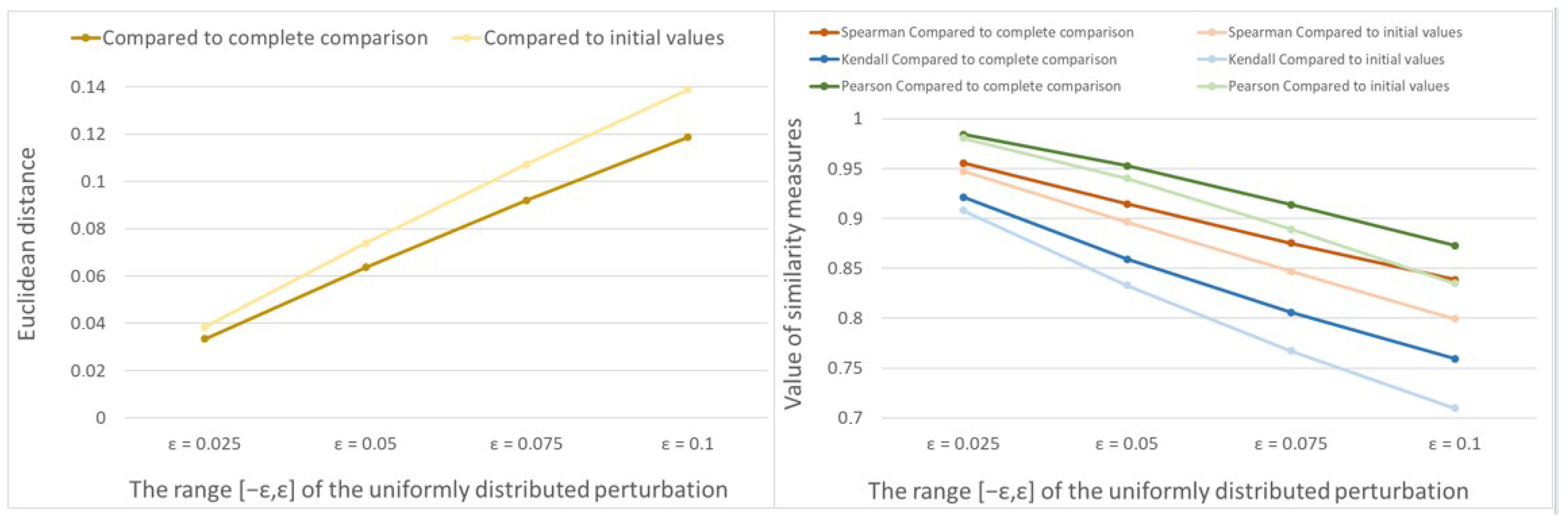
4.1. Method of Simulations

Due to the complexity of the analytical calculations, we perform Monte Carlo simulations, similar to those in [29], to examine information retrieval from incomplete comparisons in the Davidson model. This section describes the simulation methodology.

The steps of the simulations are described as follows:

• Generate a normalized random n-length $\underline{\pi }$ vector, and assign a positive $\nu$ value. The coordinates of $\underline{\pi }$ and $\nu$ are uniformly distributed random values in the interval $[0,1]$. These will be the initial parameter values for the Davidson model. $\underline{\pi }$ is referred to as the initial priority vector.
• Calculate the probabilities of the comparison results from the initial values applying formulas (1)–(3) for every possible pair. So we generate a consistent and complete data set of the comparison results.
• As we know from Theorem 2, in the case of consistent comparison data, MLE recovers the initial values in all (complete or incomplete) cases. For this reason, perturbations are performed on the consistent data set as follows: each probability value is modified by adding independent, uniformly distributed random numbers in the range [$-\epsilon$, $\epsilon$]. The $\epsilon$ value can be set between 0 and 1, but we use between 0 and 0.1. We guarantee that the resulting perturbed probability values are also between 0 and 1, then we normalize them by dividing their sum. These data serve as an inconsistent complete data set.
• Using the above perturbed probability values as a data set, the estimated $\underline{\widehat{\pi }}$ vector and $\widehat{\nu }$ value are calculated using MLE. The $\underline{\widehat{\pi }}$ vector is referred to as an estimated priority vector based on the complete comparison and is denoted by ${\underline{\widehat{\pi }}}_{co}$.
• In the next step, we calculate the estimated priority vectors for different graph structures as follows. We omit data from the complete data set. For each fixed connected graph, we keep only the data that belong to the comparison structure associated with the graph. The remaining data set is incomplete and inconsistent. After performing MLE, the estimated priority vector is called the priority vector belonging to the incomplete data set and is denoted by ${\underline{\widehat{\pi }}}_{inc}$. We want to determine how much information is retained from the initial priority vector, on the one hand, and from the estimated priority vector based on the complete comparison, on the other hand.
• The differences between the priority vectors computed from the complete and incomplete data sets for the fixed graph structure are determined using various measures.
  To analyze the similarities of the rankings, we use two rank correlations and two additional distance measures:
  • Spearman $\rho$ rank correlation

    $$\rho =1-{\displaystyle \frac{6{\sum }_{i=1}^n{d}_i^2}{n(n^2-1)}}$$

    (53)

    where $d_i$ is the difference in rankings of the ith object;
  • Kendall $\tau$ rank correlation

    $$\tau ={\displaystyle \frac{2(n_C-n_D)}{n(n-1)}}$$

    (54)

    where $n_C$ is the number of concordant pairs, and $n_D$ is the number of discordant pairs.
  • Further used distances are the Pearson correlation coefficient

    $$PE={\displaystyle \frac{{\sum }_{i=1}^n({\widehat{\pi }}_{inc,i}-{\underline{\overline{\widehat{\pi }}}}_{inc})·({\widehat{\pi }}_{co,i}-{\underline{\overline{\widehat{\pi }}}}_{co})}{\sqrt{({\sum }_{i=1}^n{({\widehat{\pi }}_{inc,i}-{\underline{\overline{\widehat{\pi }}}}_{inc})}^2))·{({\sum }_{i=1}^n({\widehat{\pi }}_{co,i})-{\underline{\overline{\widehat{\pi }}}}_{co})}^2})}}$$

    (55)

    where ${\widehat{\pi }}_{inc,i}$ is the i-th coordinate of the estimated priority vector from the incomplete comparison and ${\widehat{\pi }}_{co,i}$ is the i-th coordinate of the estimated priority vector from the complete comparison and the upper line denotes the arithmetic average of the coordinates.
    Each type of the correlation coefficients is in the interval $[-1,1]$. The closer the result is to 1, the more information is recovered about the rank or about the coordinates of the priority vector.
  • The Euclidean distance of the estimated parameter vectors

    $$EU=\sqrt{\sum _{i=1}^n{({\widehat{\pi }}_{inc,i}-{\widehat{\pi }}_{co,i})}^2}.$$

    (56)
  The Euclidean distance is always non-negative. It can be larger than 1. Its largest value is $\sqrt{2}$, if the Euclidean norms of the vectors equal 1. In this case, the smaller value represents better information retrieval.
• It is also interesting to see how much information is retained from the initial priority vector in the case of different comparison structures. In this case, both the perturbation and the omission of part of the data may cause information loss. The same similarity measures as in the previous step are used for the initial parameter set and the estimated parameter vector based on incomplete comparison. More specifically, the same similarity measures as in Step 6 are calculated according to Formulae (53)–(56), but ${\underline{\widehat{\pi }}}_{co}$ is substituted with $\underline{\pi }$.
• Repeat the above-described steps N times, where N is the number of simulations. The similarity measures described in Step 6 are random, due to the random initial parameter vector and the random perturbation value. Therefore, we take their average over the simulations for each fixed comparison structure. These average values characterize the information retrieval measures associated with the fixed comparison structures.

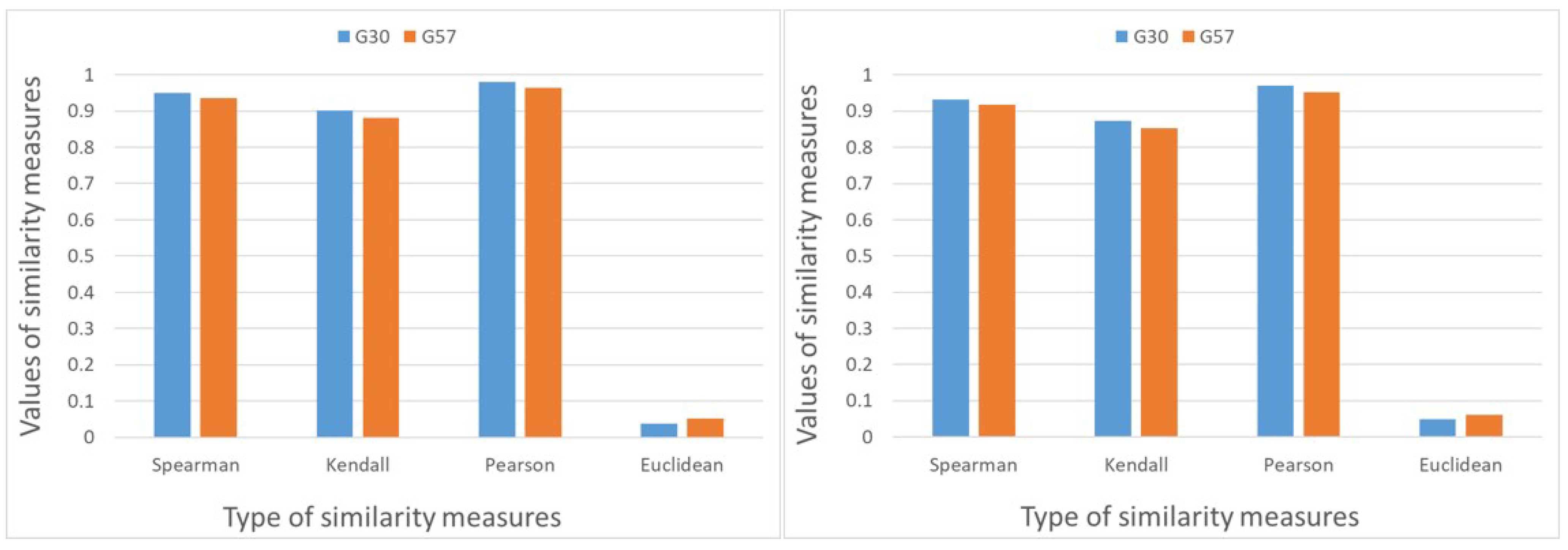
4.2. Results of Simulations in the Case of Uniformly Distributed Random Perturbation Values

As in the article [29], the numbers of objects to be compared are n = 4, 5, and 6. For four objects, six different graphs can be distinguished, including the complete comparison. For five objects, this means 21 different graphs, while for six objects, 112 different graph structures exist. The number of simulations is $N={10}^6$. The random coordinates of the initial priority vector are uniformly distributed. The perturbation values are uniformly distributed random values from the intervals $[-0.025,0.025]$, $[-0.05,0.05]$, $[-0.075,0.075]$, and $[-0.1,0.1]$.

In summary, we can conclude that the same conclusions can be drawn in the three-option Davidson model as in PCMs and in the two-option Bradley–Terry model. We illustrate these observations with a few figures.

The independence of the rankings from the similarity measures can be observed as shown in Figure 1. We experience this for all investigated ranges of the random perturbation values. This is true even if the similarity measure is computed from the initial parameter vector and the estimated parameter vector based on complete comparison. This observation confirms that most of the information retrieval is related to the graph structure.

It is important to highlight that the closer the result is to one, the more information is recovered, except for Euclidean distance, where this relationship is reversed.

We examine how the similarity measures change as a function of the range of random perturbation values when the graph structure is fixed. We find that as perturbation increases, Euclidean distances become larger, while correlations become smaller as expected. The presentation of the data for the star-graph illustrates this observation as shown in Figure 2.

In the case of $n=4$ and $n=5$,

Table 4. Average similarity measures when the distance is related to the priority vector from the complete comparison data and to the initial priority vector for $n=4$ objects and uniformly distributed random perturbation values in $[-0.1,0.1]$.

			Incomp. ${\underline{\widehat{\mathit{\pi }}}}_{\mathit{inc}}$ Versus Comp. ${\underline{\widehat{\mathit{\pi }}}}_{\mathit{co}}$				Incomp. ${\underline{\widehat{\mathit{\pi }}}}_{\mathit{inc}}$ Versus Initial $\underline{\mathit{\pi }}$
ID	|E|	Graph	$\mathsf{\rho }$	$\mathsf{\tau }$	PE	EU	$\mathsf{\rho }$	$\mathsf{\tau }$	PE	EU
1	3		0.845	0.786	0.890	0.107	0.792	0.721	0.840	0.136
2	3		0.835	0.774	0.880	0.114	0.784	0.711	0.832	0.140
3	4		0.892	0.845	0.935	0.075	0.828	0.763	0.881	0.111
4	4		0.912	0.869	0.959	0.060	0.845	0.783	0.904	0.097
5	5		0.946	0.918	0.979	0.037	0.863	0.805	0.920	0.086
6	6		1	1	1	0	0.881	0.829	0.937	0.074

and

Table 5. Average similarity measures when the distance is related to the priority vector from the complete comparison data and to the initial priority vector for n = 5 objects and uniformly distributed random perturbation values in $[-0.1,0.1]$.

			Incomp. ${\underline{\widehat{\mathit{\pi }}}}_{\mathit{inc}}$ Versus Comp. ${\underline{\widehat{\mathit{\pi }}}}_{\mathit{co}}$				Incomp. ${\underline{\widehat{\mathit{\pi }}}}_{\mathit{inc}}$ Versus Initial $\underline{\mathit{\pi }}$
ID	|E|	Graph	$\mathsf{\rho }$	$\mathsf{\tau }$	PE	EU	$\mathsf{\rho }$	$\mathsf{\tau }$	PE	EU
1	4		0.839	0.759	0.873	0.119	0.799	0.710	0.835	0.139
2	4		0.827	0.746	0.860	0.126	0.789	0.698	0.823	0.145
3	4		0.817	0.735	0.850	0.131	0.780	0.689	0.814	0.150
4	5		0.868	0.797	0.904	0.097	0.824	0.739	0.864	0.121
5	5		0.878	0.809	0.918	0.089	0.833	0.750	0.877	0.113
6	5		0.864	0.792	0.899	0.101	0.820	0.735	0.860	0.124
7	5		0.855	0.782	0.891	0.105	0.812	0.727	0.852	0.127
8	5		0.889	0.822	0.933	0.080	0.843	0.762	0.892	0.105
9	6		0.897	0.837	0.934	0.076	0.848	0.769	0.892	0.104
10	6		0.916	0.860	0.958	0.061	0.865	0.789	0.914	0.091
11	6		0.899	0.838	0.939	0.073	0.850	0.771	0.897	0.101
12	6		0.911	0.853	0.952	0.065	0.860	0.784	0.909	0.094
13	6		0.894	0.833	0.930	0.079	0.845	0.765	0.889	0.106
14	7		0.930	0.883	0.965	0.053	0.872	0.799	0.921	0.086
15	7		0.928	0.880	0.966	0.053	0.872	0.800	0.921	0.086
16	7		0.915	0.864	0.947	0.065	0.859	0.784	0.904	0.096
17	7		0.934	0.887	0.972	0.049	0.877	0.806	0.927	0.082
18	8		0.950	0.913	0.979	0.038	0.884	0.816	0.934	0.078
19	8		0.952	0.915	0.984	0.036	0.888	0.821	0.938	0.075
20	9		0.972	0.950	0.992	0.022	0.896	0.831	0.945	0.070
21	10		1	1	1	0	0.904	0.842	0.952	0.064

present the computed average similarity measures for each comparison (graph) structure with uniformly distributed random perturbation values in $[-0.1,0.1]$. The rows represent the graph structures, and the columns represent the similarity measures, with the left side showing the comparison to the estimated priority vector from the complete comparison data, and the right side showing the comparison to the initial priority vector. We can establish that every similarity measure designates the same structure as the best in the case of each comparison structure if we compare the priority vector from incomplete comparison either to the initial priority vector or to the one estimated based on the complete comparison data. In the case of the optimal comparison structures the graph structures are also represented.

The same conclusions can be stated if $n=6$.

Table 6. Optimal comparison structures and the average similarity measures belonging to them when the distance is related to the priority vector from the complete comparison data and to the initial priority vector for n = 6 objects and uniformly distributed random perturbation values in $[-0.1,0.1]$.

			Incomp. ${\underline{\widehat{\mathit{\pi }}}}_{\mathit{inc}}$ Versus Comp. ${\underline{\widehat{\mathit{\pi }}}}_{\mathit{co}}$				Incomp. ${\underline{\widehat{\mathit{\pi }}}}_{\mathit{inc}}$ Versus Initial $\underline{\mathit{\pi }}$
ID	|E|	Graph	$\mathsf{\rho }$	$\mathsf{\tau }$	PE	EU	$\mathsf{\rho }$	$\mathsf{\tau }$	PE	EU
1	5		0.837	0.743	0.860	0.123	0.805	0.703	0.828	0.139
19	6		0.874	0.789	0.910	0.092	0.839	0.742	0.876	0.110
30	7		0.900	0.825	0.937	0.075	0.861	0.771	0.901	0.096
54	8		0.917	0.849	0.953	0.063	0.875	0.790	0.917	0.086
73	9		0.934	0.876	0.969	0.051	0.889	0.809	0.932	0.077
85	10		0.943	0.890	0.975	0.045	0.895	0.817	0.937	0.073
103	11		0.952	0.905	0.981	0.038	0.901	0.825	0.943	0.069
108	12		0.962	0.923	0.988	0.031	0.908	0.835	0.950	0.065
110	13		0.971	0.941	0.992	0.024	0.912	0.841	0.953	0.062
111	14		0.984	0.966	0.996	0.015	0.916	0.847	0.957	0.060
112	15		1	1	1	0	0.920	0.853	0.961	0.057

contains the data only for the optimal graph structures, as the number of comparison structures is high. It is a very important observation that the optimal comparison structures are the same in the Davidson model, PCMs, and the BT2 model for n = 4, 5, and 6. This supports the idea that the optimal comparison structures do not depend on either the model selection or the number of options.

The simulations show that when using the best comparison structure for a given number of edges, a higher number of edges leads to better information retrieval. This holds true for all object numbers (n = 4, 5, and 6), all ranges of the uniformly distributed perturbation values, and all tested measurements.

For fixed edge numbers, Figure 3 shows the Pearson correlation and Euclidean distance belonging to the optimal structures, comparing both to the initial parameter vector and estimated parameter vector from complete comparison. Although the values differ, the tendencies coincide. It is clearly seen that the correlation values increase monotonically, while the Euclidean distances decrease monotonically as a function of the number of edges as expected. On the right side of Figure 3, the topmost value in blue is obviously zero.

As it was already established in the previous research for the BT2 model [29], although the best graph structures with k edges are always weaker than the best graph structures with $k+1$ edges, we can still find cases where the best graph structure with k edges is better than the worst graph structure with $k+1$ edges. For the Davidson model, we observe similar behavior in the data. Figure 4 illustrates this for each indicator by comparing the best graph with seven edges ($G_{30}$) and the worst graph with eight edges ($G_{57}$). The situation is the same if we compare estimated parameters arising from the incomplete and complete data, or we compare the estimated parameters arising from the incomplete comparisons to the initial parameter vector. This observation is highly significant because it supports the idea that the structure of the comparisons used to collect data matters. Therefore, using optimal comparison structures is worthwhile for better information retrieval.

We also test what can be stated for additional object numbers. Based on the simulations, we observe that for $n=7,8,9$ objects and $n-1$ compared pairs, the star graph always proves to be the best structure, while for n compared pairs, the best structure is the cycle. We suggest using these structures for $9<n$ as well.

4.3. Results of Simulations in the Case of Gaussian-Distributed Random Perturbation Values

In order to make our model more realistic, we also perform the perturbation applying Gaussian distribution. The only modification in the simulation process is made in step 3: uniformly distributed random values are changed to Gaussian-distributed random values.

In the case of $n=5$,

Table 7. Average similarity measures when the distance is related to the priority vector from the complete comparison data and to the initial priority vector for n = 5 objects and Gaussian-distributed random perturbation values with expectation 0 and dispersion 1/30.

			Incomp. ${\underline{\widehat{\mathit{\pi }}}}_{\mathit{inc}}$ Versus Comp. ${\underline{\widehat{\mathit{\pi }}}}_{\mathit{co}}$				Incomp. ${\underline{\widehat{\mathit{\pi }}}}_{\mathit{inc}}$ Versus Initial $\underline{\mathit{\pi }}$
ID	|E|	Graph	$\mathsf{\rho }$	$\mathsf{\tau }$	PE	EU	$\mathsf{\rho }$	$\mathsf{\tau }$	PE	EU
1	4		0.932	0.885	0.968	0.052	0.922	0.869	0.961	0.058
2	4		0.924	0.874	0.959	0.060	0.913	0.858	0.951	0.066
3	4		0.917	0.865	0.951	0.066	0.906	0.849	0.942	0.073
4	5		0.944	0.903	0.976	0.043	0.931	0.883	0.969	0.051
5	5		0.948	0.909	0.980	0.040	0.934	0.887	0.972	0.049
6	5		0.941	0.899	0.974	0.046	0.928	0.879	0.966	0.054
7	5		0.936	0.892	0.968	0.051	0.923	0.872	0.960	0.059
8	5		0.953	0.916	0.985	0.036	0.938	0.892	0.977	0.046
9	6		0.957	0.923	0.985	0.034	0.941	0.898	0.977	0.043
10	6		0.965	0.937	0.992	0.026	0.948	0.909	0.984	0.037
11	6		0.956	0.923	0.986	0.033	0.941	0.898	0.978	0.043
12	6		0.962	0.932	0.990	0.029	0.945	0.904	0.982	0.040
13	6		0.954	0.920	0.983	0.036	0.938	0.894	0.975	0.046
14	7		0.971	0.947	0.993	0.022	0.952	0.914	0.986	0.035
15	7		0.970	0.945	0.993	0.023	0.951	0.913	0.985	0.036
16	7		0.964	0.936	0.987	0.029	0.945	0.905	0.980	0.041
17	7		0.972	0.948	0.994	0.022	0.952	0.915	0.986	0.035
18	8		0.979	0.960	0.996	0.016	0.956	0.921	0.988	0.032
19	8		0.980	0.962	0.997	0.015	0.958	0.923	0.989	0.031
20	9		0.988	0.978	0.999	0.009	0.961	0.929	0.991	0.029
21	10		1	1	1	0	0.964	0.933	0.992	0.027

presents the computed average similarity measures for each comparison (graph) structure applying Gaussian-distributed perturbation values in $[-0.1,0.1]$. First, similarly to the uniformly distributed random perturbed values, the expectation of the perturbations is zero, but the dispersion is $1/30$. In this case, the possible values of the Gaussian-distributed random perturbation values are almost always (i.e., with probability 0.997) in the interval $[-0.1,0.1]$. The results are contained in Table 7.

The structure of Table 7 is the same as the structure of Table 5. The observations coincide with the observations in the case of uniformly distributed random perturbation, but the similarity measures are better. More precisely, Euclidean distances are smaller, and correlations are higher than in the case of uniformly distributed perturbations. In each number of compared pairs, the optimal comparison structures coincide, regardless of whether the perturbations are Gaussian-distributed or uniformly distributed random values. This observation also holds in the cases of $n=4,6$ objects.

We also investigate the case where the perturbation follows a certain tendency: its expectation is increased from zero, while the dispersion is kept at 1/30.

Table 8. Average similarity measures, when the distance is related to the priority vector from the complete comparison data and to the initial priority vector for n = 5 objects and Gaussian-distributed random perturbation values with expectation 0.01 and dispersion 1/30.

			Incomp. ${\underline{\widehat{\mathit{\pi }}}}_{\mathit{inc}}$ Versus Comp. ${\underline{\widehat{\mathit{\pi }}}}_{\mathit{co}}$				Incomp. ${\underline{\widehat{\mathit{\pi }}}}_{\mathit{inc}}$ Versus Initial $\underline{\mathit{\pi }}$
ID	|E|	Graph	$\mathsf{\rho }$	$\mathsf{\tau }$	PE	EU	$\mathsf{\rho }$	$\mathsf{\tau }$	PE	EU
1	4		0.932	0.885	0.969	0.050	0.922	0.870	0.962	0.056
2	4		0.925	0.875	0.961	0.057	0.914	0.859	0.953	0.064
3	4		0.917	0.865	0.953	0.064	0.906	0.849	0.944	0.071
4	5		0.944	0.903	0.977	0.041	0.931	0.883	0.970	0.050
5	5		0.948	0.910	0.981	0.038	0.935	0.888	0.973	0.047
6	5		0.942	0.900	0.975	0.044	0.929	0.880	0.967	0.052
7	5		0.936	0.892	0.969	0.049	0.923	0.872	0.961	0.057
8	5		0.953	0.916	0.986	0.035	0.938	0.893	0.977	0.045
9	6		0.957	0.924	0.985	0.032	0.942	0.899	0.978	0.042
10	6		0.966	0.937	0.992	0.025	0.949	0.909	0.984	0.037
11	6		0.956	0.923	0.986	0.032	0.941	0.899	0.978	0.042
12	6		0.962	0.932	0.990	0.028	0.946	0.904	0.982	0.039
13	6		0.954	0.920	0.983	0.034	0.939	0.895	0.975	0.045
14	7		0.971	0.947	0.993	0.022	0.952	0.915	0.986	0.034
15	7		0.970	0.945	0.993	0.022	0.951	0.913	0.985	0.035
16	7		0.964	0.936	0.988	0.028	0.946	0.906	0.980	0.040
17	7		0.972	0.949	0.994	0.021	0.953	0.915	0.986	0.035
18	8		0.979	0.960	0.996	0.016	0.957	0.922	0.988	0.031
19	8		0.980	0.962	0.997	0.015	0.958	0.924	0.989	0.031
20	9		0.988	0.978	0.999	0.009	0.961	0.929	0.991	0.028
21	10		1	1	1	0	0.964	0.934	0.992	0.027

presents the results in the case of Gaussian-distributed random perturbed values with mean 0.01 and standard deviation 1/30. Comparing the measurements in Table 7 and Table 8, we can see that, although the distances are usually larger and the correlations are smaller, the optimal graph structures do not change if we increase the expectation of the perturbation from zero to a positive value. Every conclusion drawn in Section 4.2 can also be repeated in the case of Gaussian-distributed perturbation with nonzero expectation. This supports the robustness of optimal graph structures.

5. Summary

The main finding of the paper is a relation between two main branches of paired comparison methods: a three-option paired comparison model with stochastic background and the multiplicative pairwise comparison matrix-based model. The key moment was the definition of consistency in PCM models. Starting with Luce’s choice axiom, we characterized the data consistency in the Davidson model. We proved that, similarly to the two-option Bradley–Terry model, in the case of consistent data in the Davidson model, the priority vector coincides with the priority vector provided by PCM, and also with the priority vector in BT2. This is not true in the case of inconsistent data. If the data are not consistent, investigating the comparison structures by simulations, we established that the same conclusions can be drawn in the case of Davidson model and the two-option Bradley–Terry model: the optimal graph structures coincide with those investigating PCMs, and these structures form a sequence presented in [29,40]. This is true both when comparing the evaluation results derived from incomplete comparisons after the perturbation to the initial priority vector, and when comparing the evaluation results derived from complete and incomplete comparisons after the perturbation, independently of the distribution of the perturbed values. Therefore, the optimal information retrieval structure does not depend on the number of options and the model.

Based on simulations for $n=4,5,6,7,8,9$, we observed that the best comparison structure is the star graph when only $n-1$ pairs are allowed for comparison, and the cycle when n pairs are allowed. Therefore, we suggest using these comparison structures when dealing with a large number n of objects and $n-1$ or n compared pairs. Further investigations would be performed in the case of the three-option Bradley–Terry and Thurstone–Mosteller models when Luce’s choice axiom is not fulfilled.

References

1. Mangla, S.K.; Kumar, P.; Barua, M.K. Risk analysis in green supply chain using fuzzy AHP approach: A case study. Resour. Conserv. Recycl. 2015, 104, 375–390. [Google Scholar] [CrossRef]
2. Shi, W. Construction and evaluation of college students’ psychological quality evaluation model based on Analytic Hierarchy Process. J. Sens. 2022, 2022, 3896304. [Google Scholar] [CrossRef]
3. Koczkodaj, W.W.; LeBrasseur, R.; Wassilew, A.; Tadeusziewicz, R. About business decision making by a consistency-driven pairwise comparisons method. J. Appl. Comput. Sci. 2009, 17, 55–70. [Google Scholar]
4. Wind, Y.; Saaty, T.L. Marketing applications of the analytic hierarchy process. Manag. Sci. 1980, 26, 641–658. [Google Scholar] [CrossRef]
5. Brunelli, M. A study on the anonymity of pairwise comparisons in group decision making. Eur. J. Oper. Res. 2019, 279, 502–510. [Google Scholar] [CrossRef]
6. Amorocho, J.A.P.; Hartmann, T. A multi-criteria decision-making framework for residential building renovation using pairwise comparison and TOPSIS methods. J. Build. Eng. 2022, 53, 104596. [Google Scholar] [CrossRef]
7. Baker, R.D.; McHale, I.G. A dynamic paired comparisons model: Who is the greatest tennis player? Eur. J. Oper. Res. 2014, 236, 677–684. [Google Scholar] [CrossRef]
8. Bozóki, S.; Csató, L.; Temesi, J. An application of incomplete pairwise comparison matrices for ranking top tennis players. Eur. J. Oper. Res. 2016, 248, 211–218. [Google Scholar] [CrossRef]
9. Baker, R.D.; McHale, I.G. Estimating age-dependent performance in paired comparisons competitions: Application to snooker. J. Quant. Anal. Sports 2024, 20, 113–125. [Google Scholar] [CrossRef]
10. Gisselquist, R.M. Paired comparison and theory development: Considerations for case selection. PS Polit. Sci. Polit. 2014, 47, 477–484. [Google Scholar] [CrossRef]
11. Crompvoets, E.A.; Béguin, A.A.; Sijtsma, K. Adaptive pairwise comparison for educational measurement. J. Educ. Behav. Stat. 2020, 45, 316–338. [Google Scholar] [CrossRef]
12. Williamson, T.B.; Watson, D.O.T. Assessment of community preference rankings of potential environmental effects of climate change using the method of paired comparisons. Clim. Change 2010, 99, 589–612. [Google Scholar] [CrossRef]
13. Verschuren, P.; Arts, B. Quantifying influence in complex decision making by means of paired comparisons. Qual. Quant. 2005, 38, 495–516. [Google Scholar] [CrossRef]
14. Tarricone, P.; Newhouse, C.P. A study of the use of pairwise comparison in the context of social online moderation. Aust. Educ. Res. 2016, 43, 273–288. [Google Scholar] [CrossRef]
15. Oliveira, I.F.; Ailon, N.; Davidov, O. A new and flexible approach to the analysis of paired comparison data. J. Mach. Learn. Res. 2018, 19, 1–29. [Google Scholar]
16. Saaty, T.L.; Vargas, L.G. The Logic of Priorities: Applications of Business, Energy, Health and Transportation; Springer Science & Business Media: Dordrecht, The Netherlands, 2013. [Google Scholar]
17. Vaidya, O.S.; Kumar, S. Analytic hierarchy process: An overview of applications. Eur. J. Oper. Res. 2006, 169, 1–29. [Google Scholar] [CrossRef]
18. Saaty, T.L. The Analytic Hierarchy Process: Planning, Priority Setting, Resource, Allocation; McGraw-Hill: New York, NY, USA, 1980. [Google Scholar]
19. Saaty, T.L. How to make a decision: The analytic hierarchy process. Eur. J. Oper. Res. 1990, 48, 9–26. [Google Scholar] [CrossRef]
20. Saaty, T.L. Decision-making with the AHP: Why is the principal eigenvector necessary. Eur. J. Oper. Res. 2003, 145, 85–91. [Google Scholar] [CrossRef]
21. Bozóki, S.; Fülöp, J.; Rónyai, L. On optimal completion of incomplete pairwise comparison matrices. Math. Comput. Model. 2010, 52, 318–333. [Google Scholar] [CrossRef]
22. Thurstone, L.L. A law of comparative judgment. Psychol. Rev. 1927, 34, 273–286. [Google Scholar] [CrossRef]
23. Bradley, R.A.; Terry, M.E. Rank analysis of incomplete block designs: I. The method of paired comparisons. Biometrika 1952, 39, 324–345. [Google Scholar] [CrossRef]
24. Glenn, W.A.; David, H.A. Ties in paired-comparison experiments using a modified Thurstone-Mosteller model. Biometrics 1960, 16, 86–109. [Google Scholar] [CrossRef]
25. Rao, P.V.; Kupper, L.L. Ties in paired-comparison experiments: A generalization of the Bradley-Terry model. J. Am. Stat. Assoc. 1967, 62, 194–204. [Google Scholar] [CrossRef]
26. Agresti, A. Analysis of ordinal paired comparison data. J. R. Stat. Soc. Ser. C Appl. Stat. 1992, 41, 287–297. [Google Scholar] [CrossRef]
27. Orbán-Mihálykó, É.; Mihálykó, C.; Koltay, L. Incomplete paired comparisons in case of multiple choice and general log-concave probability density functions. Cent. Eur. J. Oper. Res. 2019, 27, 515–532. [Google Scholar] [CrossRef]
28. Orbán-Mihálykó, É.; Koltay, L.; Szabó, F.; Csuti, P.; Kéri, R.; Schanda, J. A new statistical method for ranking of light sources based on subjective points of view. Acta Polytech. Hung. 2015, 12, 195–214. [Google Scholar]
29. Gyarmati, L.; Orbán-Mihálykó, É.; Mihálykó, C.; Szádoczki, Z.; Bozóki, S. The incomplete Analytic Hierarchy Process and Bradley–Terry model: (In)consistency and information retrieval. Expert Syst. Appl. 2023, 229, 120522. [Google Scholar] [CrossRef]
30. Davidson, R.R. On Extending the Bradley-Terry Model to Accommodate Ties in Paired Comparison Experiments. J. Am. Stat. Assoc. 1970, 65, 317–328. [Google Scholar] [CrossRef]
31. Luce, R.D. Individual Choice Behavior; Wiley: New York, NY, USA, 1959; Volume 4. [Google Scholar]
32. Luce, R.D. The choice axiom after twenty years. J. Math. Psychol. 1977, 15, 215–233. [Google Scholar] [CrossRef]
33. Mihálykó, C.; Gyarmati, L.; Orbán-Mihálykó, É.; Mihálykó, A. Evaluability of paired comparison data in stochastic paired comparison models: Necessary and sufficient condition. arXiv 2025, arXiv:2502.13617. [Google Scholar]
34. Bozóki, S.; Tsyganok, V. The (logarithmic) least squares optimality of the arithmetic (geometric) mean of weight vectors calculated from all spanning trees for incomplete additive (multiplicative) pairwise comparison matrices. Int. J. Gen. Syst. 2019, 48, 362–381. [Google Scholar] [CrossRef]
35. Kazibudzki, P.T. Redefinition of triad’s inconsistency and its impact on the consistency measurement of pairwise comparison matrix. J. Appl. Math. Comput. Mech. 2016, 15, 71–78. [Google Scholar] [CrossRef]
36. Brunelli, M. A survey of inconsistency indices for pairwise comparisons. Int. J. Gen. Syst. 2018, 47, 751–771. [Google Scholar] [CrossRef]
37. Ágoston, K.C.; Csató, L. Inconsistency thresholds for incomplete pairwise comparison matrices. Omega 2022, 108, 102576. [Google Scholar] [CrossRef]
38. Mihálykó, C.; Orbán-Mihálykó, É.; Gyarmati, L. Consistency and Inconsistency in the Case of a Stochastic Paired Comparison Model. In Proceedings of the 2024 IEEE 3rd Conference on Information Technology and Data Science (CITDS), Debrecen, Hungary, 26–28 August 2024; pp. 1–6. [Google Scholar] [CrossRef]
39. Chartier, T.P.; Harris, J.; Hutson, K.R.; Langville, A.N.; Martin, D.; Wessell, C.D. Reducing the effects of unequal number of games on rankings. IMAGE Bull. Int. Linear Algebra Soc. 2014, 52, 15–23. [Google Scholar]
40. Bozóki, S.; Szádoczki, Z. Optimal sequences for pairwise comparisons: The graph of graphs approach. arXiv 2022, arXiv:2205.08673. [Google Scholar]
Figure 1. Average correlations defined by (53) (Spearman), (54) (Kendall), (55) (Pearson), and Euclidean average distance defined by (56) for  n = 5  objects, with uniformly distributed perturbation values in  [ 0.05 , 0.05 ]  applied. The difference in the comparison of the priority vector computed from the perturbed complete data set is shown on the left, and from the initial priority vector on the right.
Mathematics 13 01374 g001
Figure 2. The Euclidean distance (on the left) and correlation values (on the right) for the star-graph are presented for different ranges of the random perturbation values, comparing the initial priority vector to the estimated priority vector from the complete data set, for  n = 5  objects.
Mathematics 13 01374 g002
Figure 3. Pearson correlation and Euclidean distance between the estimated priority vector belonging to the optimal graph structures and belonging to the complete graph and to the initial priority vector in the function of the number of graph’s edges in the case of n = 6 objects and random perturbation values uniformly distributed from the interval  [ 0.05 , 0.05 ] .
Mathematics 13 01374 g003
Figure 4. Comparison of the best graph structure with 7 edges ( G 30 ) and the worst graph structure with 8 edges ( G 57 ) in the case of n = 6 objects to compare and random perturbation values, uniformly distributed in  [ 0.05 , 0.05 ] . Differences in comparison with the estimated priority vector based on complete data on the left, differences from the initial priority vector on the right.
Mathematics 13 01374 g004