Fixed-Time Stability, Uniform Strong Dissipativity, and Stability of Nonlinear Feedback Systems

Abstract

In this paper, we develop new necessary and sufficient Lyapunov conditions for fixed-time stability that refine the classical fixed-time stability results presented in the literature by providing an optimized estimate of the settling time bound that is less conservative than the existing results. Then, building on our new fixed-time stability results, we introduce the notion of uniformly strongly dissipative dynamical systems and show that for a closed dynamical system (i.e., a system with the inputs and outputs set to zero) this notion implies fixed-time stability. Specifically, we construct a stronger version of the dissipation inequality that implies system dissipativity and generalizes the notions of strict dissipativity and strong dissipativity while ensuring that the closed system is fixed-time stable. The results are then used to derive new Kalman–Yakubovich–Popov conditions for characterizing necessary and sufficient conditions for uniform strong dissipativity in terms of the system drift, input, and output functions using continuously differentiable storage functions and quadratic supply rates. Furthermore, using uniform strong dissipativity concepts, we present several stability results for nonlinear feedback systems that guarantee finite-time and fixed-time stability. For specific supply rates, these results provide generalizations of the feedback passivity and nonexpansivity theorems that additionally guarantee finite-time and fixed-time stability. Finally, several illustrative numerical examples are provided to demonstrate the proposed fixed-time stability and uniform strong dissipativity frameworks.

1. Introduction

Finite-time convergence to a Lyapunov stable equilibrium, that is, finite-time stability, was first addressed by Roxin [1] and rigorously studied in [2,3] for time-invariant systems using continuous Lyapunov functions, whereas extensions of finite-time stability to time-varying nonlinear dynamical systems are reported in [4,5]. Specifically, Lyapunov and converse Lyapunov theorems for finite-time stability using a Lyapunov function that satisfies a scalar differential inequality involving fractional powers were established and the regularity properties of the Lyapunov function were shown to depend on the regularity properties of the settling time function capturing the finite settling time behavior of the dynamical system. An inherent drawback of finite-time stability is that the settling time function depends on the system’s initial conditions, and hence, the time of convergence to a Lyapunov stable equilibrium point may increase (possibly unboundedly) as the vector norm of the initial condition increases.

The stronger notion of fixed-time stability was developed in [6,7,8,9,10,11,12,13] to ensure convergence of the system trajectories to a finite-time stable equilibrium point in a fixed-time for any system initial condition. More specifically, the settling time function of a fixed-time stable system is uniformly bounded regardless of the system initial conditions, and hence, a fixed-time stable system is finite-time stable with a settling-time function that is bounded on the whole domain by a finite value. Building on the original work of Polyakov [7,12], the authors in [13] develop a new sufficient fixed-time stability theorem that gives a less conservative estimate of the system settling time as compared to the results of [7]. Additional refinements involving necessary and sufficient conditions for fixed-time stability that take into account the regularity properties of the settling time function are presented in [12].

While Lyapunov stability theory forms the cornerstone for addressing the stability properties of closed systems (i.e., systems described by a flow that evolve without any inputs), dissipativity theory builds on Lyapunov theory to address open (i.e., input–state–output) system properties by exploiting the notion that numerous physical dynamical systems have certain input, state, and output properties related to conservation, dissipation, and transport of mass and energy. Dissipative dynamical systems provide fundamental connections between physics, dynamical systems theory, and control science and engineering. Using an input–state–output system description based on generalized system energy considerations that uses a state-space formalism to link engineering systems with memory to well-known physical phenomena, dissipative systems have been extensively developed in the literature to provide a general framework for the analysis and design of control systems [14,15,16].

In this paper, we first develop new necessary and sufficient conditions for fixed-time stability of nonlinear systems with continuous vector fields using a Lyapunov function that satisfies a scalar differential inequality that serves to refine the classical fixed-time stability result of [7] as well as the more recent result in [13]. While our fixed-time stability result resembles the results given in [7,13], our result provides an optimized estimate of the fixed time bound that is less conservative than the results reported in [7,13]. Furthermore, unlike [7,13], we also provide necessary conditions for fixed-time stability and show that the regularity properties of the Lyapunov function and those of the settling time function are related, and hence, our converse Lyapunov result assures the existence of a continuous Lyapunov function for systems with forward complete solutions.

Next, building on the recent results of [17], we develop the notion of uniform strong dissipativity by constructing a stronger version of the dissipation hypothesis that implies system dissipativity and generalizes the notions of strict dissipativity [16] and strong dissipativity [17] while ensuring that the closed system is fixed-time stable. Moreover, we develop necessary and sufficient Kalman–Yakubovich–Popov conditions in terms of the system drift, input, and output functions for characterizing uniform strong dissipativity via continuously differentiable storage functions and quadratic supply rates. In the case where the supply rate is taken as the net system power or the weighted input–output energy, the Kalman–Yakubovich–Popov conditions provide generalizations to passivity and nonexpansivity for characterizing uniform strong passivity and uniform strong nonexpansivity.

Finally, given that one of the most important applications of dissipativity theory is the fundamental role it plays in addressing stability of nonlinear feedback systems [16,18], we use the concepts of uniform strong dissipativity for nonlinear dynamical systems with appropriate storage functions and supply rates, to construct continuously differentiable Lyapunov functions for nonlinear feedback interconnections by appropriately combining the storage functions for the forward and feedback subsystems. General stability criteria are given for Lyapunov, asymptotic, finite-time, and fixed-time stability for feedback interconnections of nonlinear dynamical systems. These results generalize the feedback interconnection results of [16,18], and for power and input–output energy supply rates they provide extensions of the classical feedback passivity and nonexpansivity theorems to additionally guarantee finite-time and fixed-time stability.

2. Fixed-Time Stability of Nonlinear Dynamical Systems

Consider the closed nonlinear dynamical system given by

$$\dot{x}=f\left(x\left(t\right)\right),x\left(t_0\right)=x_0,t\in {\mathcal{I}}_{x_0},$$

(1)

where $x\left(t\right)\in \mathcal{D}\subseteq {\mathbb{R}}^n$, $t\in {\mathcal{I}}_{x_0}$, is the system state vector, ${\mathcal{I}}_{x_0}$ is the maximal interval of existence of a solution $x\left(t\right)$ of (1), $\mathcal{D}$ is an open set, $0\in \mathcal{D}$, $f\left(0\right)=0$, and $f(·)$ is continuous on $\mathcal{D}$. A continuously differentiable function $x:{\mathcal{I}}_{x_0}\to \mathcal{D}$ is said to be a solution of (1) on the interval ${\mathcal{I}}_{x_0}\subseteq \mathbb{R}$ if $x(·)$ satisfies (1) for all $t\in {\mathcal{I}}_{x_0}$. Since f is continuous on $\mathcal{D}$, it follows from Peano’s theorem ([16], Thm. 2.24) that, for every $x\in \mathcal{D}$, there exists ${\tau }_0<0<{\tau }_1$ and a solution $x(·)$ of (1) defined on $({\tau }_0,{\tau }_1)$ such that $x\left(t_0\right)=x_0$. A solution $x(·)$ is right maximally defined if x cannot be extended on the right (either uniquely or nonuniquely) to a solution of (1). Recall that every solution of (1) has a solution which is right maximally defined, and if $x:[t_0,\tau )\to \mathcal{D}$ is a right maximally defined solution of (1) such that, for all $t\in [t_0,\tau )$, $x\left(t\right)\in {\mathcal{D}}_{\mathrm{c}}$, where ${\mathcal{D}}_{\mathrm{c}}\subset \mathcal{D}$ is compact, then $\tau =\infty$ ([19], pp. 17–18).

We assume that (1) possesses unique solutions in forward time for all initial conditions except possibly the origin in the following sense. For every $x\in \mathcal{D}\setminus \left\{0\right\}$ there exists ${\tau }_x>0$ such that, if $y_1:[0,{\tau }_1)\to \mathcal{D}$ and $y_2:[0,{\tau }_2)\to \mathcal{D}$ are two solutions of (1) with $y_1\left(0\right)=y_2\left(0\right)=x$, then ${\tau }_x\le min\{{\tau }_1,{\tau }_2\}$ and $y_1\left(t\right)=y_2\left(t\right)$ for all $t\in [0,{\tau }_x)$. Without loss of generality, we assume that for each x, ${\tau }_x$ is chosen to be the largest such number in the set of nonnegative real numbers ${\overline{\mathbb{R}}}_{+}$. In this case, we denote the trajectory or, alternatively, the unique solution curve of (1) on $[t_0,{\tau }_x)$ by $s(·,x)\triangleq s^x(·)$ satisfying $s(t_0,x)=x$. In this paper, we use the notation $s(t,x)$, $t\in {\mathcal{I}}_x$, and $x(·)$ interchangeably to denote the solution of (1) with initial condition $x\left(0\right)=x$.

Recall that if ${\tau }_x<\infty$ and ${lim}_{t\to {\tau }_x}x\left(t\right)$ exists, then $s(t,x)$ approaches the boundary $\partial \mathcal{D}$ of $\mathcal{D}$ or 0 as $t\to {\tau }_x$ ([19], Thm. I.2.1). Hence, $s^x(·)$ cannot be extended on the right uniquely to a solution of (1) since in the former case $s^x(·)$ cannot be extended to the right, whereas in the latter case solutions starting at zero result in extended right solutions of (1) in more than one way. Thus, if (1) admits nonunique solutions in forward time for $x\left(0\right)=0$, then the map $s(·,·)$ is defined as $s:{\mathbb{R}}_{+}\times \mathcal{D}\setminus \left\{0\right\}\to \mathcal{D}\setminus \left\{0\right\}$, whereas if (1) possesses a unique solution for $x\left(0\right)=x$ for every $x\in \mathcal{D}$, then the map $s(·,·)$ is defined as $s:{\mathbb{R}}_{+}\times \mathcal{D}\to \mathcal{D}$ and $s^x:[0,{\tau }_x)\to \mathcal{D}$ is the unique right maximally defined solution of (1), where ${\mathbb{R}}_{+}$ denotes the set of positive real numbers. Sufficient conditions for forward uniqueness in the absence of Lipschitz continuity can be found in [20,21,22,23].

Next, we recall the definition for finite-time stability given in [2]. For this definition, ${\mathcal{B}}_{\epsilon }\left(x\right)$ denotes the open ball centered at x with radius $\epsilon$ in the Euclidean norm.

Definition 1. 

Consider the nonlinear dynamical system (1). The zero solution$x\left(t\right)\equiv 0$ to (1) is finite-time stable if there exists an open neighborhood $\mathcal{N}\subseteq \mathcal{D}$ of the origin and a function $T:\mathcal{N}\setminus \left\{0\right\}\to (0,\infty )$, called the settling time function, such that the following statements hold:

$\left(i\right)$

Finite-time convergence. For every $x\in \mathcal{N}\setminus \left\{0\right\}$, $s^x\left(t\right)$ is defined on $[0,T(x\left)\right)$, $s^x\left(t\right)\in \mathcal{N}\setminus \left\{0\right\}$ for all $t\in [0,T(x\left)\right)$, and ${lim}_{t\to T\left(x\right)}s(t,x)=0$.

$\left(ii\right)$

Lyapunov stability. For every $\epsilon >0$ there exists $\delta >0$ such that ${\mathcal{B}}_{\delta }\left(0\right)\subset \mathcal{N}$ and, for every $x\in {\mathcal{B}}_{\delta }\left(0\right)\setminus \left\{0\right\}$, $s(t,x)\in {\mathcal{B}}_{\epsilon }\left(0\right)$ for all $t\in [0,T(x\left)\right)$.

The zero solution $x\left(t\right)\equiv 0$ to (1) is globally finite-time stable if it is finite-time stable with $\mathcal{N}=\mathcal{D}={\mathbb{R}}^n$.

Theorem 1 

([2]). Consider the nonlinear dynamical system (1). Assume that there exists a continuously differentiable function $V:\mathcal{D}\to \mathbb{R}$, real numbers $a>0$ and $\alpha \in (0,1)$, and a neighborhood $\mathcal{M}\subseteq \mathcal{D}$ of the origin such that

$$\begin{array}{cc}\hfill V\left(0\right)& =0,\hfill \end{array}$$

(2)

$$\begin{array}{cc}\hfill V\left(x\right)& >0,x\in \mathcal{M}\setminus \left\{0\right\},\hfill \end{array}$$

(3)

$$\begin{array}{cc}\hfill V^{\prime }\left(x\right)f\left(x\right)& \le -a{\left(V\left(x\right)\right)}^{\alpha },x\in \mathcal{M}\setminus \left\{0\right\}.\hfill \end{array}$$

(4)

Then the zero solution $x\left(t\right)\equiv 0$ to (1) is finite-time stable. Moreover, there exist an open neighborhood $\mathcal{N}$ of the origin and a settling-time function $T:\mathcal{N}\to [0,\infty )$ such that

$$T\left(x_0\right)\le {\displaystyle \frac{1}{a(1-\alpha )}}{\left(V\left(x_0\right)\right)}^{1-\alpha },x_0\in \mathcal{N},$$

(5)

and $T(·)$ is continuous on $\mathcal{N}$. If, in addition, $\mathcal{N}=\mathcal{D}={\mathbb{R}}^n$, $V(·)$ is radially unbounded, and (3) and (4) hold on ${\mathbb{R}}^n\setminus \left\{0\right\}$, then the zero solution $x\left(t\right)\equiv 0$ to (1) is globally finite-time stable.

Remark 1. 

As shown in [2], Theorem 1 implies that for a dynamical system possessing a finite-time stable equilibrium and a discontinuous settling time function there does not exist a Lyapunov function satisfying the hypothesis of Theorem 1. However, in the case where the settling time function is continuous, Theorem 1 is also necessary for the existence of a continuous function $V:\mathcal{D}\to \mathbb{R}$ satisfying (2) and (3), and (4) holding with $V^{\prime }\left(x\right)f\left(x\right)$ replaced by the upper-right Dini derivative of V.

Next, we recall the notion of fixed-time stability given in [12].

Definition 2. 

The zero solution $x\left(t\right)\equiv 0$ to (1) is fixed-time stable if there exists an open neighborhood $\mathcal{N}\subseteq \mathcal{D}$ of the origin and a settling-time function $T:\mathcal{N}\setminus \left\{0\right\}\to (0,\infty )$ such that the following statements hold:

$\left(i\right)$

Finite-time stability. The zero solution $x\left(t\right)\equiv 0$ to (1) is finite-time stable.

$\left(ii\right)$

Uniform boundedness of the settling time function. For every $x\in \mathcal{N}$, there exists $T_{max}>0$ such that $T\left(x\right)\le T_{max}$.

The zero solution $x\left(t\right)\equiv 0$ to (1) is globally fixed-time stable if it is fixed-time stable with $\mathcal{N}=\mathcal{D}={\mathbb{R}}^n$.

The following example presents a fixed-time stable system and is used in the proof of Theorem 2.

Example 1. 

Consider the scalar nonlinear dynamical system given by

$$\dot{z}\left(t\right)=-{\mathrm{sign}\left(z\right)[a|z\left(t\right)|}^{\delta }+{b|z\left(t\right)|}^{\theta }{]}^k-cz\left(t\right),z\left(0\right)=z_0,t\ge 0,$$

(6)

where $z\left(t\right)\in \mathbb{R}$, $\mathrm{sign}\left(\sigma \right)\triangleq \sigma /|\sigma |$, $\sigma \ne 0$, and $\mathrm{sign}\left(0\right)\triangleq 0$, and $a,b,c,\theta ,k>0,\delta \ge 0$ are constants such that $\delta k<1$ and $\theta k>1$. Note that the right-hand side of (6) is continuous everywhere and locally Lipschitz everywhere except the origin. Hence, for every initial condition in $\mathbb{R}$, (6) has a unique solution in forward time on a sufficiently small interval.

Next, rewriting (6) as

$${\displaystyle \frac{\mathrm{sign}\left(z\right)\mathrm{d}z}{{[a|z\left(t\right)|}^{\delta }+{b|z\left(t\right)|}^{\theta }{]}^k+c|z|}}=-\mathrm{d}t$$

and defining

$$\varphi \left(z\right)\triangleq {\int }_0^z{\displaystyle \frac{\mathrm{sign}\left(z\right)\mathrm{d}z}{{\left[{a|z\left(t\right)|}^{\delta }+b{|z\left(t\right)|}^{\theta }\right]}^k+c|z|}},$$

it follows that $\varphi \left(z\right(t\left)\right)-\varphi \left(z\right(0\left)\right)=-t$, which implies $\varphi \left(z\right(t\left)\right)=\varphi \left(z\right(0\left)\right)-t$. Now, since $\varphi \left(z\right)=0$ if and only if $z=0$,

$$\underset{t\to T\left(z_0\right)}{lim}z\left(t\right)=0,$$

where the settling time function $T:\mathbb{R}\to {\mathbb{R}}_{+}$ is given by

$$T\left(z_0\right)=\varphi \left(z_0\right)={\int }_0^{z_0}{\displaystyle \frac{\mathrm{sign}\left(z\right)\mathrm{d}z}{{\left[{a|z\left(t\right)|}^{\delta }+b{|z\left(t\right)|}^{\theta }\right]}^k+c|z|}}.$$

(7)

Note that T is continuous but not Lipschitz continuous at the origin. It is clear from (7) that (i) of Definition 1 is satisfied with $\mathcal{N}=\mathcal{D}=\mathbb{R}$. Now, Lyapunov stability follows by considering the Lyapunov function $V\left(z\right)=z^2$. Thus, the zero solution $z\left(t\right)\equiv 0$ to (6) is globally finite-time stable.

Next, to show fixed-time stability note that $T(·)$ has even symmetry and is increasing for $z\in {\mathbb{R}}_{+}$, and hence,

$$\begin{array}{cc}\hfill T\left(z\right)\le \underset{z_0\to \infty }{lim}T\left(z_0\right)& ={\int }_0^{\infty }{\displaystyle \frac{\mathrm{d}z}{{(a{z}^{\delta }+b{z}^{\theta })}^k+cz}}\hfill \\ \hfill & ={\int }_0^r{\displaystyle \frac{\mathrm{d}z}{{(a{z}^{\delta }+b{z}^{\theta })}^k+cz}}+{\int }_r^{\infty }{\displaystyle \frac{\mathrm{d}z}{{(a{z}^{\delta }+b{z}^{\theta })}^k+cz}}\hfill \\ \hfill & \le {\int }_0^r{\displaystyle \frac{\mathrm{d}z}{a^k{z}^{\delta k}+cz}}+{\int }_r^{\infty }{\displaystyle \frac{\mathrm{d}z}{b^k{z}^{\theta k}+cz}},\hfill \end{array}$$

(8)

where $r\in {\mathbb{R}}_{+}$ is arbitrary and finite. Using the transformation $v=z^{1-\delta k}$, the first integral in (8) gives

$$\begin{array}{cc}\hfill {\int }_0^r{\displaystyle \frac{\mathrm{d}z}{a^k{z}^{\delta k}+cz}}& ={\displaystyle \frac{1}{1-\delta k}}{\int }_0^{r^{1-\delta k}}{\displaystyle \frac{z^{\delta k}\mathrm{d}v}{a^k{z}^{\delta k}+cz}}\hfill \\ \hfill & ={\displaystyle \frac{1}{1-\delta k}}{\int }_0^{r^{1-\delta k}}{\displaystyle \frac{\mathrm{d}v}{a^k+cv}}\hfill \\ \hfill & ={\displaystyle \frac{1}{(1-\delta k)c}}ln\left(1+{\displaystyle \frac{c}{a^k}}{r}^{1-\delta k}\right),\hfill \end{array}$$

whereas using the transformation $u=z^{1-\theta k}$, the second integral in (8) gives

$$\begin{array}{cc}\hfill {\int }_r^{\infty }{\displaystyle \frac{\mathrm{d}z}{b^k{z}^{\theta k}+cz}}& =-{\displaystyle \frac{1}{\theta k-1}}{\int }_{r^{1-\theta k}}^0{\displaystyle \frac{z^{\theta k}\mathrm{d}u}{b^k{z}^{\theta k}+cz}}\hfill \\ \hfill & =-{\displaystyle \frac{1}{\theta k-1}}{\int }_{r^{1-\theta k}}^0{\displaystyle \frac{\mathrm{d}u}{b^k+cu}}\hfill \\ \hfill & ={\displaystyle \frac{1}{(\theta k-1)c}}ln\left(1+{\displaystyle \frac{c}{b^k}}{r}^{1-\theta k}\right).\hfill \end{array}$$

Thus,

$$\underset{z_0\to \infty }{lim}T\left(z_0\right)\le {\displaystyle \frac{1}{(1-\delta k)c}}ln\left(1+{\displaystyle \frac{c}{a^k}}{r}^{1-\delta k}\right)+{\displaystyle \frac{1}{(\theta k-1)c}}ln\left(1+{\displaystyle \frac{c}{b^k}}{r}^{1-\theta k}\right)\triangleq g\left(r\right).$$

(9)

Now, computing ${\displaystyle \frac{\mathrm{d}g\left(r\right)}{\mathrm{d}r}}$ and setting it to zero gives

$$\begin{array}{cc}\hfill 0& ={\displaystyle \frac{\mathrm{d}g\left(r\right)}{\mathrm{d}r}}\hfill \\ \hfill & ={\displaystyle \frac{r^{-\delta k}}{a^k+c{r}^{1-\delta k}}}-{\displaystyle \frac{r^{-\theta k}}{b^k+c{r}^{1-\theta k}}}\hfill \\ \hfill & =a^k{r}^{-\theta k}+c{r}^{1-\delta k-\theta k}-b^k{r}^{-\delta k}-c{r}^{1-\delta k-\theta k}\hfill \\ \hfill & =a^k{r}^{-\theta k}-b^k{r}^{-\delta k},\hfill \end{array}$$

whereas a similar calculation shows that ${\displaystyle \frac{{\mathrm{d}}^{2}g}{\mathrm{d}{r}^2}}>0$, $r\in {\mathbb{R}}_{+}$, which implies that $g\left(r\right)$ attains its minimum value at $r_{min}={\left({\displaystyle \frac{a}{b}}\right)}^{1/(\theta -\delta )}$. Hence, with $r=r_{min}$, (9) gives

$$T\left(z_0\right)\le {\displaystyle \frac{1}{(1-\delta k)c}}ln\left[1+{\displaystyle \frac{c}{a^k}}{\left({\displaystyle \frac{a}{b}}\right)}^{{\displaystyle \frac{1-\delta k}{\theta -\delta }}}\right]+{\displaystyle \frac{1}{(\theta k-1)c}}ln\left[1+{\displaystyle \frac{c}{b^k}}{\left({\displaystyle \frac{b}{a}}\right)}^{{\displaystyle \frac{\theta k-1}{\theta -\delta }}}\right].$$

(10)

Thus, the zero solution $z\left(t\right)\equiv 0$ to (6) is globally fixed-time stable.

Next, we present sufficient conditions for fixed-time stability of (1) using a Lyapunov function that satisfies a new scalar differential inequality that refines the fixed-time stability results of [7,13].

Theorem 2. 

Consider the nonlinear dynamical system (1). Assume that there exist a continuously differentiable function $V:\mathcal{D}\to {\overline{\mathbb{R}}}_{+}$, real numbers $a,b,c,\delta ,\theta ,k>0$ such that $\delta k<1$ and $\theta k>1$, and a neighborhood $\mathcal{M}\subseteq \mathcal{D}$ of the origin such that

$$\begin{array}{cc}\hfill V\left(0\right)& =0,\hfill \end{array}$$

(11)

$$\begin{array}{cc}\hfill V\left(x\right)& >0,x\in \mathcal{M}\setminus \left\{0\right\},\hfill \end{array}$$

(12)

$$\begin{array}{cc}\hfill V^{\prime }\left(x\right)f\left(x\right)& \le -{\left[a{V}^{\delta }\left(x\right)+b{V}^{\theta }\left(x\right)\right]}^k-cV\left(x\right),x\in \mathcal{M}\setminus \left\{0\right\}.\hfill \end{array}$$

(13)

Then the zero solution $x\left(t\right)\equiv 0$ to (1) is fixed-time stable. Moreover, there exist an open neighborhood $\mathcal{N}$ of the origin and a settling-time function $T:\mathcal{N}\to [0,\infty )$ such that, for all $x_0\in \mathcal{N}$,

$$T\left(x_0\right)\le T_{max}\triangleq {\displaystyle \frac{1}{(1-\delta k)c}}ln\left[1+{\displaystyle \frac{c}{a^k}}{\left({\displaystyle \frac{a}{b}}\right)}^{{\displaystyle \frac{1-\delta k}{\theta -\delta }}}\right]+{\displaystyle \frac{1}{(\theta k-1)c}}ln\left[1+{\displaystyle \frac{c}{b^k}}{\left({\displaystyle \frac{b}{a}}\right)}^{{\displaystyle \frac{\theta k-1}{\theta -\delta }}}\right],$$

(14)

where $T(·)$ is continuous on $\mathcal{N}$. If, in addition, $\mathcal{N}=\mathcal{D}={\mathbb{R}}^n$, $V(·)$ is radially unbounded, and (12) and (13) hold on ${\mathbb{R}}^n\setminus \left\{0\right\}$, then the zero solution $x\left(t\right)\equiv 0$ to (1) is globally fixed-time stable.

Proof. 

First note that since $V(·)$ is positive definite and

$$\begin{array}{cc}\hfill V^{\prime }\left(x\right)f\left(x\right)& \le -{\left[a{V}^{\delta }\left(x\right)+b{V}^{\theta }\left(x\right)\right]}^k-cV\left(x\right)\hfill \\ \hfill & \le -a^k{V}^{\delta k}\left(x\right),x\in \mathcal{M}\setminus \left\{0\right\},\hfill \end{array}$$

where $\delta k<1$, it follows from Theorem 1 that the zero solution $x\left(t\right)\equiv 0$ to (1) is finite-time stable and $T(·)$ is continuous on $\mathcal{N}$.

Next, it follows from Example 1 and Theorem 4.16 of [16], with $w\left(z\right)=-{(a{z}^{\delta }+b{z}^{\theta })}^k-cz$ and $z\left(t\right)=s(t,V\left(x_0\right))$, that

$$V\left(x\left(t\right)\right)\le s(t,V\left(x_0\right)),x_0\in {\mathcal{B}}_{\delta }\left(0\right),t\in [0,\infty ),$$

(15)

where $s(·,·)$ is the trajectory of (6) with $z\left(0\right)=V\left(x_0\right)$. Now, it follows from (9), (15), and the positive definiteness of $V(·)$ that

$$x\left(t\right)=0,t\ge T\left(x_0\right),$$

where

$$\underset{x_0}{sup}T\left(x_0\right)\le {\displaystyle \frac{1}{(1-\delta k)c}}ln\left[1+{\displaystyle \frac{c}{a^k}}{\left({\displaystyle \frac{a}{b}}\right)}^{{\displaystyle \frac{1-\delta k}{\theta -\delta }}}\right]+{\displaystyle \frac{1}{(\theta k-1)c}}ln\left[1+{\displaystyle \frac{c}{b^k}}{\left({\displaystyle \frac{b}{a}}\right)}^{{\displaystyle \frac{\theta k-1}{\theta -\delta }}}\right].$$

Hence, the zero solution $x\left(t\right)\equiv 0$ to (1) is fixed-time stable.

Finally, if $\mathcal{N}=\mathcal{D}={\mathbb{R}}^n$ and $V(·)$ is radially unbounded, then global fixed-time stability follows using standard arguments as used in proving global asymptotic stability. □

It is important to note here that the proof of fixed-time stability in Theorem 2 also follows from Theorem 5 of [12] with $r\left(V\left(x\right)\right)={\left[a{V}^{\delta }\left(x\right)+b{V}^{\theta }\left(x\right)\right]}^k+cV\left(x\right)$. However, the settling time bound provided by Theorem 5 of [12] does not directly yield the explicit uniform fixed time bound (14) for the settling time function $T\left(x_0\right)$. Furthermore, Theorem 5 of [12] assumes that the Lyapunov function V is continuously differentiable, whereas Theorem 2 also holds for the more general case where $V:\mathcal{D}\to {\mathbb{R}}_{+}$ is continuous and $\delta >0$ is relaxed to $\delta \ge 0$. In this case, we need to replace the Lie derivative $V^{\prime }\left(x\right)f\left(x\right)$ in (13) by the upper-right Dini derivative of V along the trajectories of (1) given by the ${\overline{\mathbb{R}}}_{+}$-valued function

$$\dot{V}\left(x\right)=\left(D^{+}(V\circ s^x)\right)\left(0\right),$$

(16)

where “∘” denotes the composition operator and

$$\left(D^{+}(V\circ s^x)\right)\left(t\right)=\dot{V}\left(s(t,x)\right)=\underset{h\to 0^{+}}{\lim \sup }{\displaystyle \frac{1}{h}}[V\left(s(t+h,x)\right)-V\left(s(t,x)\right)].$$

(17)

Note that $\dot{V}\left(x\right)$ is defined for every $x\in \mathcal{D}$ for which $s^x$ is defined, and if for $x=0$, $\dot{V}\left(0\right)$ is defined, then $\dot{V}\left(0\right)=0$.

To see that Theorem 2 holds in this case, note that it follows from Theorem 4.16 of [16], with $w\left(z\right)=-{(a{z}^{\delta }+b{z}^{\theta })}^k-cz$ and $z\left(t\right)=s(t,V\left(x_0\right))$, that

$$V\left(x\left(t\right)\right)\le s(t,V\left(x_0\right)),x_0\in {\mathcal{B}}_{\delta }\left(0\right),t\in [0,\infty ),$$

(18)

where $s(·,·)$ is the trajectory of (6) with $z\left(0\right)=V\left(x_0\right)$. Next, it follows from (7) that $V\left(x\right(t\left)\right)=0$ for all $t\ge T\left(x_0\right)$, where the settling time function $T:\mathcal{N}\to {\mathbb{R}}_{+}$ given by

$$T\left(x\right)={\int }_0^{V\left(x\right)}{\displaystyle \frac{\mathrm{d}z}{{(a{z}^{\delta }+b{z}^{\theta })}^k+cz}}$$

is continuous at $x=0$.

Now, define $W:\mathcal{N}\to {\mathbb{R}}_{+}$ by

$$W\left(x\right)\triangleq {\left(T\left(x\right)\right)}^{{\displaystyle \frac{1}{1-\alpha }}}={\left({\int }_0^{V\left(x\right)}{\displaystyle \frac{\mathrm{d}z}{{(a{z}^{\delta }+b{z}^{\theta })}^k+cz}}\right)}^{{\displaystyle \frac{1}{1-\alpha }}},$$

where $\alpha \in (0,1)$, and note that W is continuous and positive definite, and by the fact that $s\left(T\right(x)+t,x)=0$, $\dot{W}\left(0\right)=0$. Hence, for all $x\in \mathcal{N}\setminus \left\{0\right\}$, it follows from Proposition 2.4 of [2] that $W\circ s^x$ is continuously differentiable on $[0,T(x\left)\right)$ so that (16) can be easily computed as

$$\dot{W}\left(x\right)={\displaystyle \frac{1}{1-\alpha }}{\left({\int }_0^{V\left(x\right)}{\displaystyle \frac{\mathrm{d}z}{{(a{z}^{\delta }+b{z}^{\theta })}^k+cz}}\right)}^{{\displaystyle \frac{\alpha }{1-\alpha }}}{\displaystyle \frac{1}{{[a{V}^{\delta }\left(x\right)+b^{\theta }V\left(x\right)]}^k+cV\left(x\right)}}\dot{V}\left(x\right).$$

Now, using (13), with $V^{\prime }\left(x\right)f\left(x\right)$ replaced by $\dot{V}\left(x\right)$, we obtain

$$\begin{array}{cc}\hfill \dot{W}\left(x\right)& \le -{\displaystyle \frac{1}{1-\alpha }}{\left({\int }_0^{V\left(x\right)}{\displaystyle \frac{\mathrm{d}z}{{(a{z}^{\delta }+b{z}^{\theta })}^k+cz}}\right)}^{{\displaystyle \frac{\alpha }{1-\alpha }}}\hfill \\ \hfill & =-{\displaystyle \frac{1}{1-\alpha }}{\left(W\left(x\right)\right)}^{\alpha },x\in \mathcal{N}\setminus \left\{0\right\}.\hfill \end{array}$$

Hence, it follows from Theorem 4.2 of [2] that the zero solution $x\left(t\right)\equiv 0$ to (1) is finite-time stable. Uniform boundedness of the settling time function follows identically as in the proof of Theorem 2, and hence, fixed-time stability holds in the case where $V:\mathcal{D}\to {\mathbb{R}}_{+}$ is continuous and $\delta \ge 0$.

In the limiting case where $c\to 0$, Theorem 2 specializes to the fixed-time stability result given in [13] for the case where f is continuous and V is continuously differentiable. (It is important to note here, however, that [13] addresses nonlinear systems of the form given by (1) wherein $f:{\mathbb{R}}^n\to {\mathbb{R}}^n$ is Lebesgue measurable and locally essentially bounded with respect to x.) To see this, first note that in this case (13) specializes to Equation (7) of [13] and (14) gives

$$\begin{array}{cc}\hfill T_{max,2}& =\underset{c\to 0}{lim}\left[{\displaystyle \frac{1}{(1-\delta k)c}}ln\left(1+{\displaystyle \frac{c}{a^k}}{\left({\displaystyle \frac{a}{b}}\right)}^{{\displaystyle \frac{1-\delta k}{\theta -\delta }}}\right)+{\displaystyle \frac{1}{(\theta k-1)c}}ln\left(1+{\displaystyle \frac{c}{b^k}}{\left({\displaystyle \frac{b}{a}}\right)}^{{\displaystyle \frac{\theta k-1}{\theta -\delta }}}\right)\right]\hfill \\ \hfill & ={\displaystyle \frac{1}{(1-\delta k)}}{\displaystyle \frac{1}{a^k}}{\left({\displaystyle \frac{a}{b}}\right)}^{{\displaystyle \frac{1-\delta k}{\theta -\delta }}}\underset{c\to 0}{lim}{\displaystyle \frac{1}{\left(1+\frac{c}{a^k}{\left(\frac{a}{b}\right)}^{\frac{1-\delta k}{\theta -\delta }}\right)}}\hfill \\ \hfill & +{\displaystyle \frac{1}{(\theta k-1)}}{\displaystyle \frac{1}{b^k}}{\left({\displaystyle \frac{b}{a}}\right)}^{{\displaystyle \frac{\theta k-1}{\theta -\delta }}}\underset{c\to 0}{lim}{\displaystyle \frac{1}{\left(1+\frac{c}{b^k}{\left(\frac{b}{a}\right)}^{\frac{\theta k-1}{\theta -\delta }}\right)}}\hfill \\ \hfill & ={\displaystyle \frac{1}{(1-\delta k)}}{\displaystyle \frac{1}{a^k}}{\left({\displaystyle \frac{a}{b}}\right)}^{{\displaystyle \frac{1-\delta k}{\theta -\delta }}}+{\displaystyle \frac{1}{(\theta k-1)}}{\displaystyle \frac{1}{b^k}}{\left({\displaystyle \frac{b}{a}}\right)}^{{\displaystyle \frac{\theta k-1}{\theta -\delta }}}\hfill \\ \hfill & ={\displaystyle \frac{1}{a^k}}{\left({\displaystyle \frac{a}{b}}\right)}^{{\displaystyle \frac{1-\delta k}{\theta -\delta }}}\left({\displaystyle \frac{1}{1-\delta k}}+{\displaystyle \frac{1}{\theta k-1}}\right),\hfill \end{array}$$

where we use L’H$\widehat{\mathrm{o}}$pital’s rule to evaluate the indeterminate form limits in the first equality. Note that $T_{max,2}$ is the settling time bound given in [13]. However, since, for $z>0$, $ln(1+z)<z$, it follows that

$$\begin{array}{cc}\hfill T_{max}& <{\displaystyle \frac{1}{(1-\delta k)c}}{\displaystyle \frac{c}{a^k}}{\left({\displaystyle \frac{a}{b}}\right)}^{{\displaystyle \frac{1-\delta k}{\theta -\delta }}}+{\displaystyle \frac{1}{(\theta k-1)c}}{\displaystyle \frac{c}{b^k}}{\left({\displaystyle \frac{b}{a}}\right)}^{{\displaystyle \frac{\theta k-1}{\theta -\delta }}}\hfill \\ \hfill & ={\displaystyle \frac{1}{a^k}}{\left({\displaystyle \frac{a}{b}}\right)}^{{\displaystyle \frac{1-\delta k}{\theta -\delta }}}\left({\displaystyle \frac{1}{1-\delta k}}+{\displaystyle \frac{1}{\theta k-1}}\right)\hfill \\ \hfill & =T_{max,2},\hfill \end{array}$$

(19)

which shows that Theorem 2 provides a sharper bound on the settling time function as compared to the results reported in [13] for a continuous vector field f.

Alternatively, setting $r=1$ in (9) and considering the limiting case as $c\to 0$ we recover the fixed-time stability result of Polyakov [7]. To see this, note that in this case (13) specializes to the differential inequality given in Lemma 1 of [7] with the settling time bound

$$\begin{array}{cc}\hfill T_{max,3}& =\underset{c\to 0}{lim}\left[{\displaystyle \frac{1}{(1-\delta k)c}}ln\left(1+{\displaystyle \frac{c}{a^k}}\right)+{\displaystyle \frac{1}{(\theta k-1)c}}ln\left(1+{\displaystyle \frac{c}{b^k}}\right)\right]\hfill \\ \hfill & ={\displaystyle \frac{1}{(1-\delta k)}}{\displaystyle \frac{1}{a^k}}\underset{c\to 0}{lim}{\displaystyle \frac{1}{\left(1+\frac{c}{a^k}\right)}}+{\displaystyle \frac{1}{(\theta k-1)}}{\displaystyle \frac{1}{b^k}}\underset{c\to 0}{lim}{\displaystyle \frac{1}{\left(1+\frac{c}{b^k}\right)}}\hfill \\ \hfill & ={\displaystyle \frac{1}{a^k(1-\delta k)}}+{\displaystyle \frac{1}{b^k(\theta k-1)}}.\hfill \end{array}$$

Since $r=1$ is not the minimum of $g\left(r\right)$ defined in (9), it follows from (19) that

$$T_{max}<T_{max,2}\le T_{max,3}·$$

Example 2. 

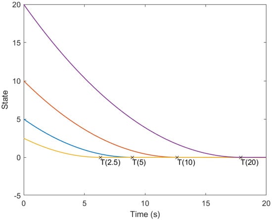
In this example, we show the stark difference in the conservatism of the settling time bound estimate between our fixed-time stability result and the results of [7,13]. To see this, we consider the scalar nonlinear system (6) given in Example 1 and we first consider the case where $b=c=0$, $a=0.5$, and $\delta k=0.5$, which results in a finite-time stable system. Figure 1 shows the solutions $z\left(t\right)$ versus time for different initial conditions and clearly shows that the settling time function increases as the initial conditions increase.

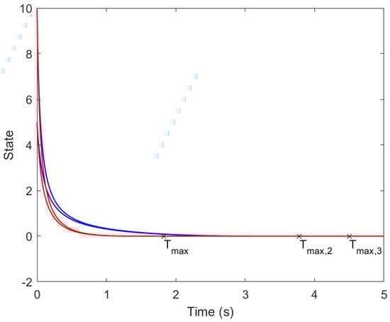
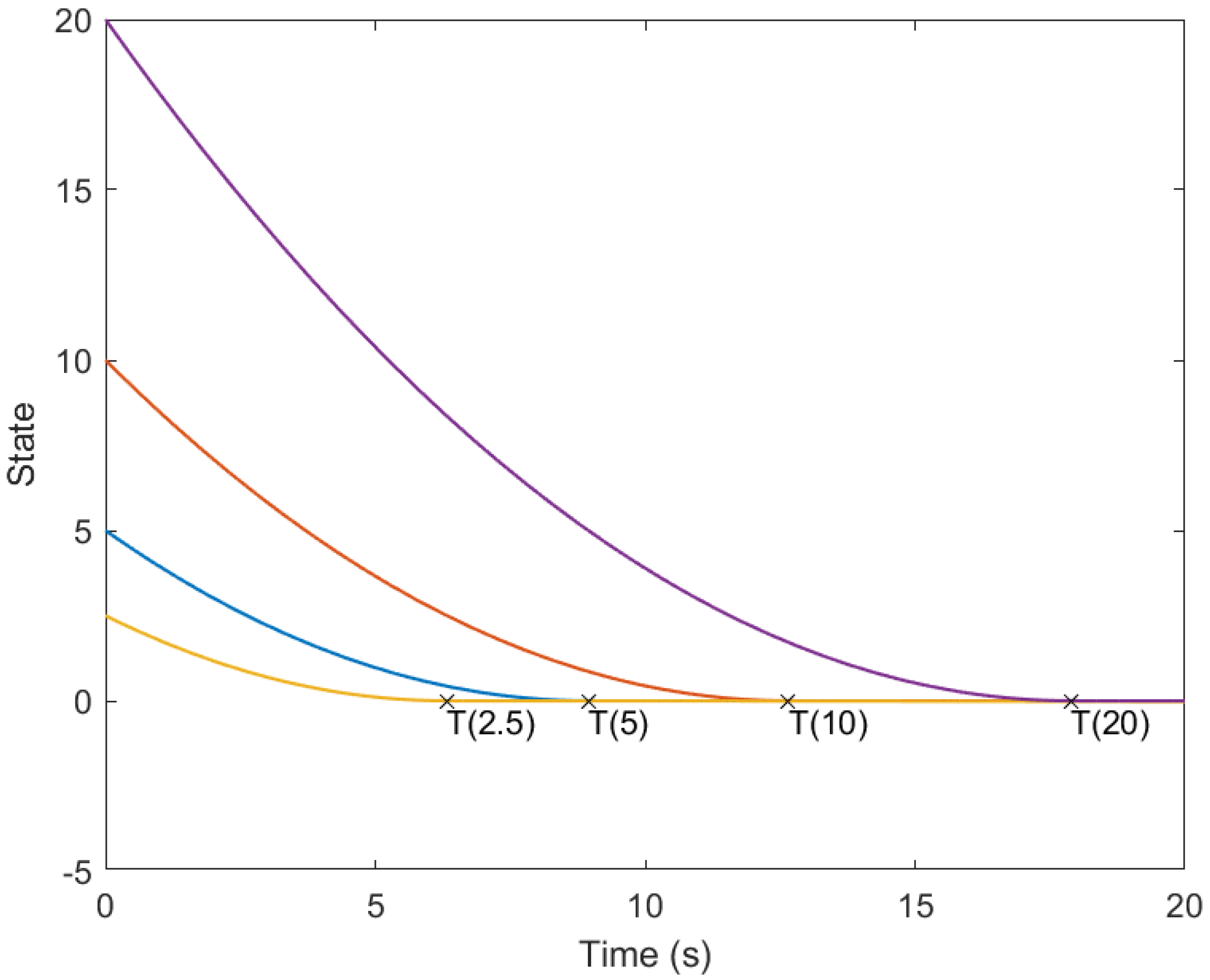
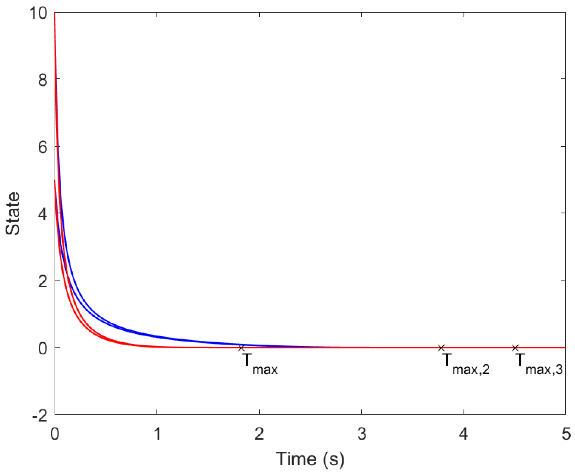
Next, we consider (6) where $a=0.5$, $b=2$, $c=3$, $\delta k=0.5$, and $\theta k=2$, which results in a fixed-time stable system. Figure 2 shows the solutions $z\left(t\right)$ versus time of (6) for different initial conditions as well as the settling time bound estimates predicted by Theorem 2$(c=3,r=0.397)$ as well as the estimates predicted by [13]$(c=0,r=0.397)$ and [7]$(c=0,r=1)$. It is clear from Figure 2 that Theorem 2 provides a less conservative estimate for the settling time bound as compared to the estimates provided by [7,13].

Next, we provide a 2-dimensional example that demonstrates the difference in the settling time estimates provided by [7,13].

Example 3. 

In this example, we show the difference in the conservatism of the settling time bound between our fixed-time stability result and the results of [7,13] for a controlled system. Consider the nonlinear controlled dynamical system given by

$$\begin{array}{cc}\hfill {\dot{x}}_1\left(t\right)& =-\mathrm{sign}\left(x_1\left(t\right)\right){|x_1\left(t\right)|}^{0.5}-x_1{\left(t\right)}^3-x_1\left(t\right)+x_2\left(t\right),x_1\left(0\right)=x_{10},t\ge 0,\hfill \end{array}$$

(20)

$$\begin{array}{cc}\hfill {\dot{x}}_2\left(t\right)& =-x_1\left(t\right)-x_2\left(t\right)+u\left(t\right),x_2\left(0\right)=x_{20},\hfill \end{array}$$

(21)

where

$$u=-\mathrm{sign}\left(x_2\right){|x_2|}^{0.5}-x_2^3.$$

(22)

To show that the closed-loop system (20)–(22) is fixed-time stable, consider the Lyapunov function candidate $V(x_1,x_2)=x_1^2+x_2^2={\parallel x\parallel }_2^2$, where $x={[x_1{x}_2]}^{\mathrm{T}}$, and note that

$$\begin{array}{cc}\hfill \dot{V}\left(x\right)& =-2|x_1{|}^{1.5}-2{|x_2|}^{1.5}-2x_1^4-2x_2^4-2x_1^2-2x_2^2\hfill \\ \hfill & =-{2\parallel x\parallel }_{1.5}^{1.5}-{2\parallel x\parallel }_4^4-2{\parallel x\parallel }_2^2\hfill \\ \hfill & \le -{2\parallel x\parallel }_2^{1.5}-{\parallel x\parallel }_2^4-2{\parallel x\parallel }_2^2\hfill \\ \hfill & =-2{\left(V\left(x\right)\right)}^{0.75}-{\left(V\left(x\right)\right)}^2-2V\left(x\right),x\in {\mathbb{R}}^2.\hfill \end{array}$$

Thus, it follows from Theorem 2, with $a=2$, $b=1$, $c=2$, $k=1$, $\delta =0.75$, and $\theta =2$, that the zero solution $x\left(t\right)\equiv 0$ of the closed-loop system (20)–(22) is globally fixed-time stable with a settling time bound $T_{max}=1.7831$ s.

Next, note that

$$\begin{array}{cc}\hfill \dot{V}\left(x\right)& \le -2{\left(V\left(x\right)\right)}^{0.75}-{\left(V\left(x\right)\right)}^2-2V\left(x\right)\hfill \\ \hfill & \le -2{\left(V\left(x\right)\right)}^{0.75}-{\left(V\left(x\right)\right)}^2,x\in {\mathbb{R}}^2,\hfill \end{array}$$

which shows that the scalar differential Lyapunov inequalities for guaranteeing fixed-time stability reported in [7,13] hold with the same $V\left(x\right)$ and the same constants. Using Corollary 1 of [13] and Lemma 1 of [7] we compute the settling time bounds as $T_{max,2}=2.8717$ s and $T_{max,3}=3$ s.

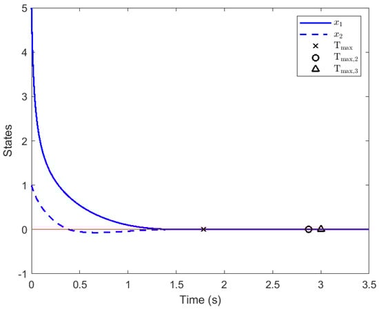
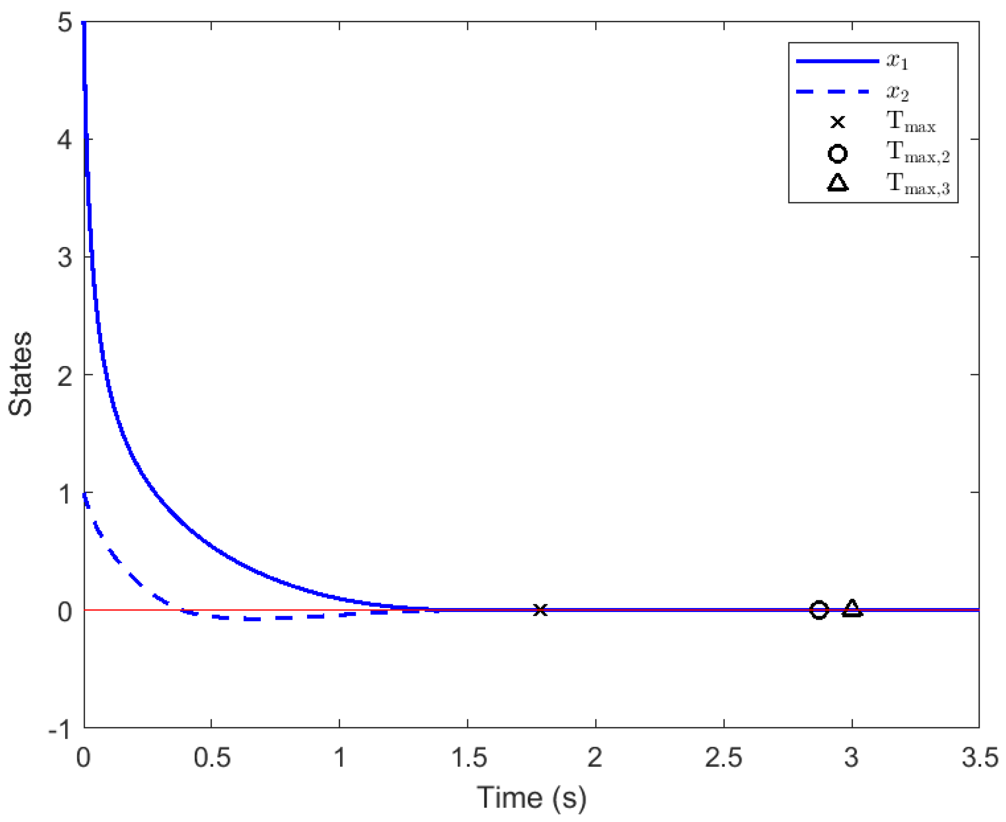
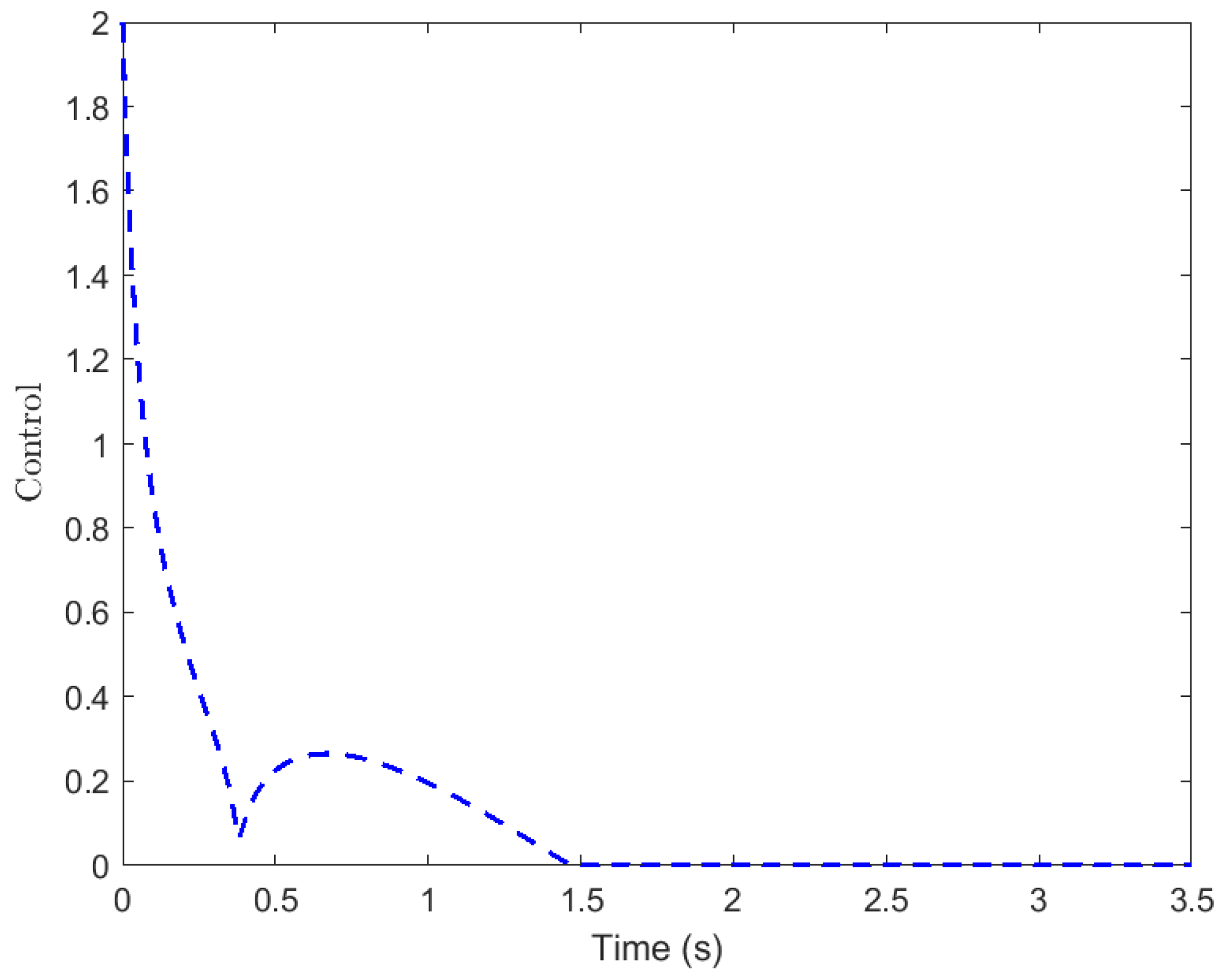
Figure 3 and Figure 4 show the closed-loop system trajectories and the control input versus time along with the settling time bound estimate for each result. Note that Theorem 2 provides a less conservative estimate for the settling time bound than predicted by [7,13] with the same control effort.

Example 4. 

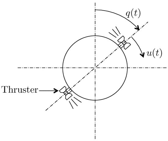
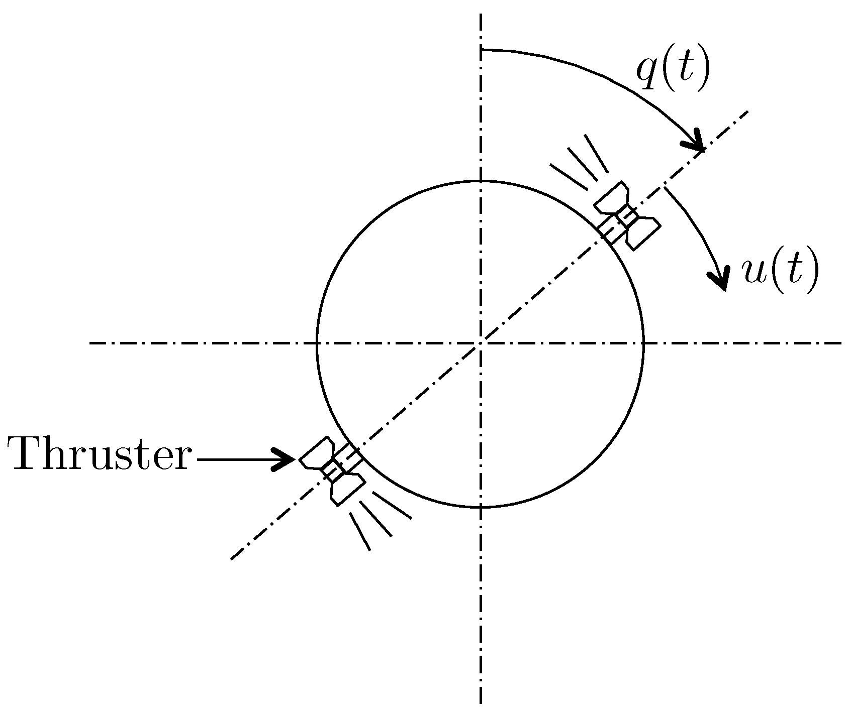
To demonstrate the use of Theorem 2 for fixed-time stabilization, consider the rigid satellite shown in Figure 5. The satellite is assumed to be in a frictionless environment and rotates about an axis perpendicular to the page. A torque $u\left(t\right)\in \mathbb{R}$, $t\ge 0$, is applied to the satellite by firing the thrusters shown in the figure resulting in the equation of motion $J\ddot{q}\left(t\right)=u\left(t\right)$, where $t\ge 0$, J is the mass moment of inertia of the satellite, $q\left(t\right)\in \mathbb{R}$ is the angular rotation in rad, $\dot{q}\left(t\right)\in \mathbb{R}$ is the angular velocity in rad/s, and $q\left(0\right)=q_0\in \mathbb{R}$ and $\dot{q}\left(0\right)=p_0\in \mathbb{R}$ are the initial conditions. Taking $x_1\left(t\right)\triangleq q\left(t\right)$ and $x_2\left(t\right)=\dot{q}\left(t\right)$, and setting $J=1$ $kg·m^2$ the dynamics can be written in the state space form as

$$\begin{array}{cc}\hfill {\dot{x}}_1\left(t\right)& =x_2\left(t\right),x_1\left(0\right)=x_{10},t\ge 0,\hfill \end{array}$$

(23)

$$\begin{array}{cc}\hfill {\dot{x}}_2\left(t\right)& =u\left(t\right),x_2\left(0\right)=x_{20}.\hfill \end{array}$$

(24)

Consider the continuous feedback control law $u=\psi (x_1,x_2)=u_1(x_1,x_2)+u_2(x_1,x_2)$, where

$$\begin{array}{cc}\hfill u_1(x_1,x_2)& =-\mathrm{sign}\left(x_1\right)|x_1{|}^{{\displaystyle \frac{\alpha }{2-\alpha }}}-\mathrm{sign}\left(x_2\right){|x_2|}^{\alpha },\hfill \end{array}$$

(25)

$$\begin{array}{cc}\hfill u_2(x_1,x_2)& =-\mathrm{sign}\left(x_1\right)|x_1{|}^{{\displaystyle \frac{4-3\alpha }{2-\alpha }}}-\mathrm{sign}\left(x_2\right){|x_2|}^{{\displaystyle \frac{4-3\alpha }{3-2\alpha }}},\hfill \end{array}$$

(26)

and $\alpha \in (0,1)$. Furthermore, consider the Lyapunov function candidate

$$\begin{array}{cc}\hfill V(x_1,x_2)& ={\displaystyle \frac{k_1(2-\alpha )}{3-\alpha }}|x_1{|}^{{\displaystyle \frac{3-\alpha }{2-\alpha }}}+k_2{x}_1{x}_2+{\displaystyle \frac{1}{3-\alpha }}{|x_2|}^{3-\alpha }\hfill \\ \hfill & +{\displaystyle \frac{k_1^{\prime }(2-\alpha )}{(3-2\alpha )(3-\alpha )}}|x_1{|}^{{\displaystyle \frac{(3-2\alpha )(3-\alpha )}{2-\alpha }}}+{\displaystyle \frac{k_2^{\prime }}{(3-2\alpha )}}\mathrm{sign}\left(x_1\right){|x_1|}^{3-2\alpha }{x}_2\hfill \\ \hfill & +{\displaystyle \frac{k_2^{\prime }(3-2\alpha )}{(3-\alpha )(3-2\alpha )-(2-\alpha )}}\mathrm{sign}\left(x_2\right){|x_2|}^{3-\alpha -{\displaystyle \frac{2-\alpha }{3-2\alpha }}}{x}_1,\hfill \end{array}$$

where $k_1=1.5$, $k_2=0.3$, $k_1^{\prime }=1.5$, and $k_2^{\prime }=0.3$, and note that $V(·,·)$ is continuously differentiable everywhere. Next, using homogeneity theory [3,24] and after a considerable amount of algebraic manipulation (see [24] for a similar analysis) it can be shown that $V(·,·)$ is positive definite and satisfies the conditions of Theorem 2. Hence, the zero solution $(x_1\left(t\right),x_2\left(t\right))\equiv (0,0)$ of (23) and (24) with $u=\psi (x_1,x_2)$ is globally fixed-time stable.

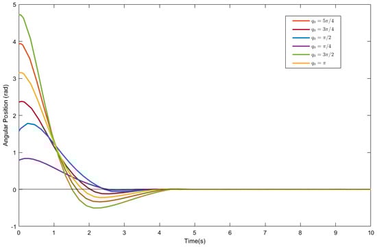
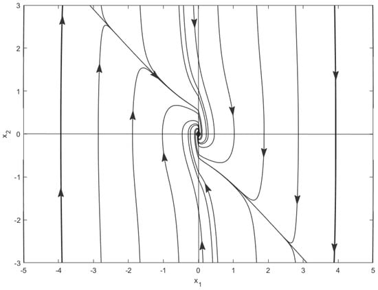
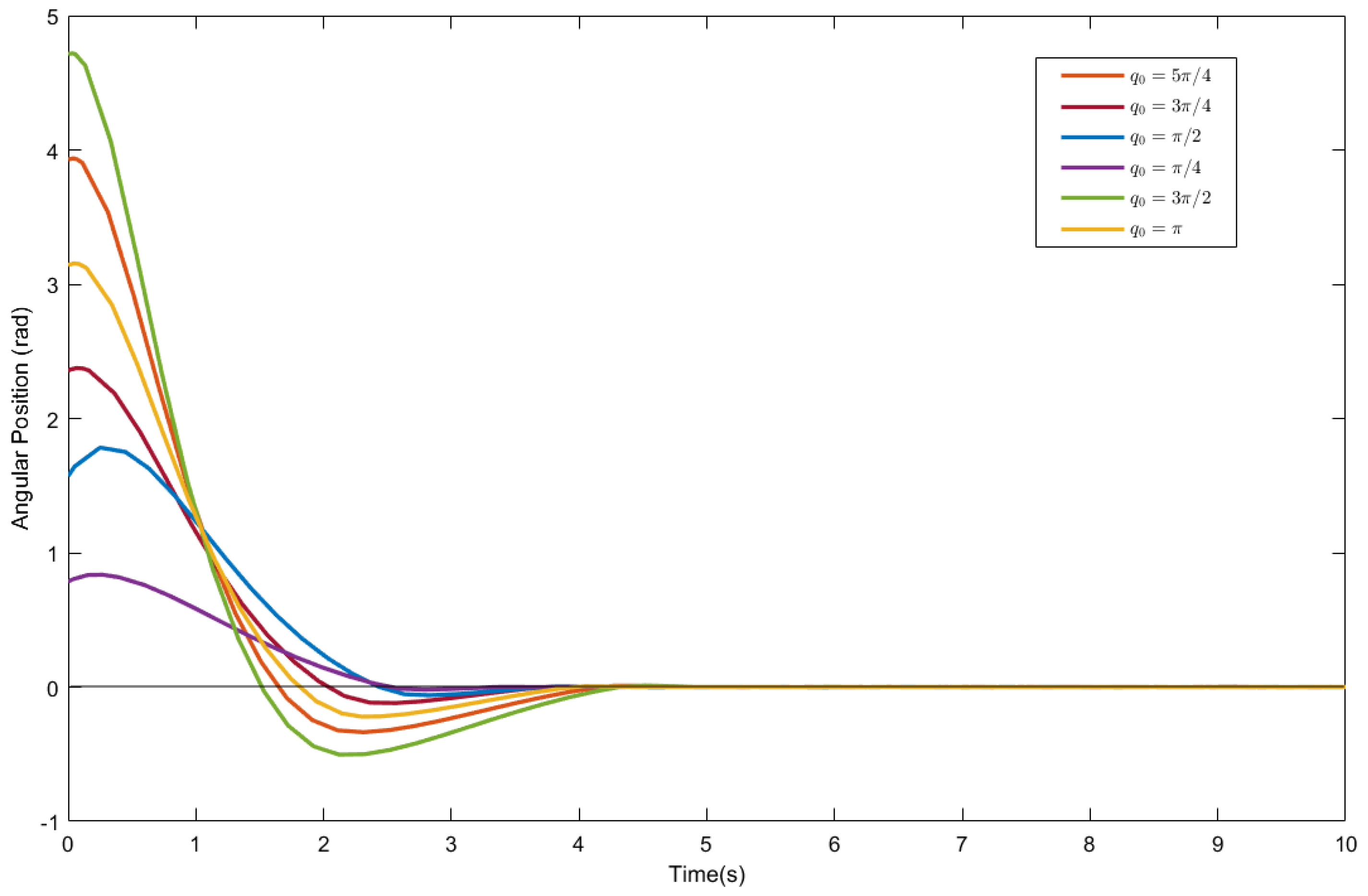
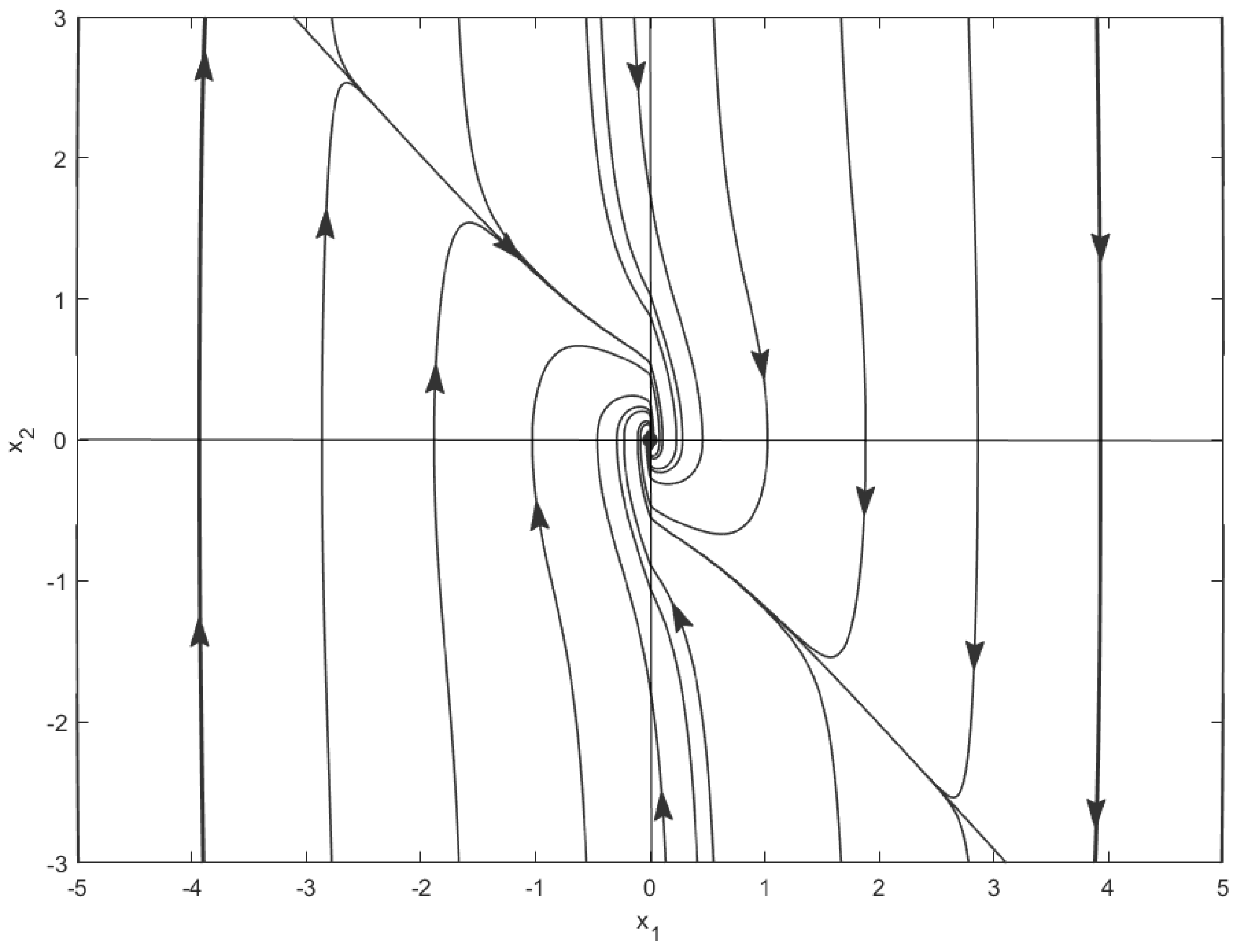
Figure 6 shows the controlled satellite angular position for an initial angular velocity $p_0=\pi /6$ rad/s and different initial angular positions. The phase portrait for the closed-loop system (23) and (24) with feedback $u=\psi (x_1,x_2)$ is shown in Figure 7. The phase portrait shows that the closed-loop system trajectories converge to a positively invariant terminal sliding mode in fixed time. Thus, the controller $u=\psi (x_1,x_2)$ provides an example of sliding mode control without using discontinuous or high-gain feedback.

Finally, we present a converse theorem for fixed-time stability in the case where the settling time function is continuous. For the statement of the result, recall the definition of the upper-right Dini derivative of a given continuous function $V:\mathcal{D}\to \mathbb{R}$ along the trajectories of (1) given by (16).

Theorem 3. 

Let $\mathcal{N}\subseteq \mathcal{D}$ be an open neighborhood of the origin. If the zero solution $x\left(t\right)\equiv 0$ to (1) is fixed-time stable and the settling time function $T(·)$ is continuous at $x=0$, then there exist a continuous function $V:\mathcal{N}\to \mathbb{R}$ and scalars $a,b,c,\delta ,\theta ,k>0$ such that $\delta k<1$ and $\theta k>1$, and $V\left(0\right)=0$, $V\left(x\right)>0$, $x\in \mathcal{N}$, $x\ne 0$, and

$$\dot{V}\left(x\right)\le -{[a{V}^{\delta }\left(x\right)-b{V}^{\theta }\left(x\right)]}^k-cV\left(x\right),x\in \mathcal{N}.$$

(27)

Proof. 

First, note that since fixed-time stability implies finite-time stability it follows from Proposition 2.4 of [2] that the settling time function $T:\mathcal{N}\to {\mathbb{R}}_{+}$ is continuous. Since (1) is fixed-time stable, there exists $T_{max}>0$ such that, for every $x\in \mathcal{N}$, $T\left(x\right)\le T_{max}$. Now, define $V:\mathcal{N}\to {\mathbb{R}}_{+}$ by

$$V\left(x\right)\triangleq {\left({\displaystyle \frac{T\left(x\right)}{T_{max}}}\right)}^{{\displaystyle \frac{1}{1-\delta }}},$$

where $\delta \in (0,1)$. Note that since $V(·)$ is continuous and positive definite, and by $s\left(T\right(x)+t,x)=0$, $x\in \mathcal{N}$ and $t\in {\mathbb{R}}_{+}$, $\dot{V}\left(0\right)=0$. Since $T\left(s\right(t,x\left)\right)=max\left\{T\right(x)-t,0\}$, $x\in \mathcal{N}$, $t\in {\mathbb{R}}_{+}$, it follows that $V\circ s^x$ is continuously differentiable on $[0,T(x\left)\right)$, and hence, (16) can be computed as

$$\begin{array}{cc}\hfill \dot{V}\left(x\right)& =-{\displaystyle \frac{1}{(1-\delta )T_{max}}}{\left({\displaystyle \frac{T\left(x\right)}{T_{max}}}\right)}^{{\displaystyle \frac{\delta }{1-\delta }}}\hfill \\ \hfill & =-{\displaystyle \frac{1}{3(1-\delta )T_{max}}}\left[{\left({\displaystyle \frac{T\left(x\right)}{T_{max}}}\right)}^{{\displaystyle \frac{\delta }{1-\delta }}}+{\left({\displaystyle \frac{T\left(x\right)}{T_{max}}}\right)}^{{\displaystyle \frac{\delta }{1-\delta }}}+{\left({\displaystyle \frac{T\left(x\right)}{T_{max}}}\right)}^{{\displaystyle \frac{\delta }{1-\delta }}}\right]\hfill \\ \hfill & \le -{\displaystyle \frac{1}{3(1-\delta )T_{max}}}\left[{\left({\displaystyle \frac{T\left(x\right)}{T_{max}}}\right)}^{{\displaystyle \frac{\delta }{1-\delta }}}+{\left({\displaystyle \frac{T\left(x\right)}{T_{max}}}\right)}^{{\displaystyle \frac{\theta }{1-\delta }}}+\left({\displaystyle \frac{T\left(x\right)}{T_{max}}}\right)\right]\hfill \\ \hfill & =-{\displaystyle \frac{1}{3(1-\delta )T_{max}}}\left[{\left(V\left(x\right)\right)}^{\delta }+{\left(V\left(x\right)\right)}^{\theta }+V\left(x\right)\right],\hfill \end{array}$$

(28)

where $\theta >1$ and the inequality in (28) follows from the fact that, for all $x\in \mathcal{N}$, ${\displaystyle \frac{T\left(x\right)}{T_{max}}}\le 1$ and that, for all $z\in (0,1)$ and $p>1>q$, $z^p<z<z^q$. Hence, $\dot{V}(·)$ is continuous and negative definite on $\mathcal{N}$ and satisfies (27) with $a=b=c={\displaystyle \frac{1}{3(1-\delta )T_{max}}}$ and $k=1$. □

Theorem 3 shows that the regularity properties for the existence of a continuous Lyapunov function satisfying the fixed-time scalar differential inequality (27) strongly depend on the regularity properties of the settling time function. A converse theorem involving a continuously differentiable Lyapunov function satisfying an alternative scalar differential inequality for fixed-time stability of (1) for the more restrictive case wherein (1) possesses well-defined solutions in forward and backward time for all $x_0\in \mathcal{N}\setminus \left\{0\right\}$ is given by Theorem 7 of [12].

3. Strongly and Uniformly Strongly Dissipative Dynamical Systems

In this section, we extend the notions of dissipativity [16] and strong dissipativity [17] to introduce the notion of uniform strong dissipativity. Consider the nonlinear dynamical system $\mathcal{G}$ given by

$$\begin{array}{ccc}\hfill \dot{x}\left(t\right)& =& F(x\left(t\right),u\left(t\right)),x\left(t_0\right)=x_0,t\ge t_0,\hfill \end{array}$$

(29)

$$\begin{array}{ccc}\hfill y\left(t\right)& =& H\left(x\right(t),u(t\left)\right),\hfill \end{array}$$

(30)

where, for every $t\ge 0$, $x\left(t\right)\in \mathcal{D}\subseteq {\mathbb{R}}^n$, $\mathcal{D}$ is an open set with $0\in \mathcal{D}$, $u\left(t\right)\in U\subseteq {\mathbb{R}}^m$ with $0\in U$, $y\left(t\right)\in Y\subseteq {\mathbb{R}}^l$, $F:\mathcal{D}\times U\to {\mathbb{R}}^n$, and $H:\mathcal{D}\times U\to Y$. We assume that $F(·,·)$ and $H(·,·)$ are continuous mappings. For the dynamical system $\mathcal{G}$ given by (29) and (30) defined on the state space $\mathcal{D}$, $\mathcal{U}$ and $\mathcal{Y}$ define an input and output space, respectively, consisting of continuous bounded U-valued and Y-valued functions on the semi-infinite interval $[0,\infty )$. The set U contains the set of input values, that is, for every $u(·)\in \mathcal{U}$ and $t\in [0,\infty )$, $u\left(t\right)\in U$. The set Y contains the set of output values, that is, for every $y(·)\in \mathcal{Y}$ and $t\in [0,\infty )$, $y\left(t\right)\in Y$.

The spaces $\mathcal{U}$ and $\mathcal{Y}$ are assumed to be closed under the shift operator, that is, if $u(·)\in \mathcal{U}$ (resp., $y(·)\in \mathcal{Y}$), then the function defined by $u_T\stackrel{▵}{=}u(t+T)$ (resp., $y_T\stackrel{▵}{=}y(t+T)$) is contained in $\mathcal{U}$ (resp., $\mathcal{Y}$) for every $T\ge 0$. Furthermore, for the nonlinear dynamical system $\mathcal{G}$ we assume that the required properties for the existence and uniqueness of solutions are satisfied, that is, $u(·)$ satisfies sufficient regularity conditions such that the system (29) has a unique solution forward in time.

For the dynamical system $\mathcal{G}$ given by (29) and (30), a function $r:U\times Y\to \mathbb{R}$ such that $r(0,0)=0$ is called a supply rate [14] if it is locally integrable, that is, for every $t\in [t_0,\infty )$ and input–output pairs $u\left(t\right)\in U$ and $y\left(t\right)\in Y$ satisfying (29) and (30), $r(·,·)$ satisfies

$${\int }_{t_1}^{t_2}|r(u\left(s\right),y\left(s\right))|\mathrm{d}s<\infty ,t_2\ge t_1\ge 0.$$

The following definition extends the notions of dissipativity [16] and strong dissipativity [17] to uniform strong dissipativity.

Definition 3. 

A dynamical system $\mathcal{G}$ of the form (29) and (30) is dissipative with respect to the supply rate $r(u,y)$ if there exists a continuous nonnegative-definite function $V_{\mathrm{s}}:\mathcal{D}\to \mathbb{R}$, called a storage function, such that the dissipation inequality

$$V_{\mathrm{s}}\left(x\left(t\right)\right)\le V_{\mathrm{s}}\left(x\left(t_0\right)\right)+{\int }_{t_0}^{t}r(u\left(s\right),y\left(s\right))\mathrm{d}s$$

(31)

is satisfied for all $t\ge t_0\ge 0$, where $x(·)$ is the solution of (29) with $u\left(t\right)\in U$. A dynamical system $\mathcal{G}$ of the form (29) and (30) is strongly dissipative with respect to the supply rate $r(u,y)$ if there exist constants $a>0$ and $\alpha \in (0,1),$ and a continuous nonnegative-definite function $V_{\mathrm{s}}:\mathcal{D}\to \mathbb{R}$ such that the strong dissipation inequality

$$V_{\mathrm{s}}\left(x\left(t\right)\right)+a{\int }_{t_0}^t{V}_{\mathrm{s}}^{\alpha }\left(x\left(s\right)\right)\mathrm{d}s\le V_{\mathrm{s}}\left(x\left(t_0\right)\right)+{\int }_{t_0}^{t}r(u\left(s\right),y\left(s\right))\mathrm{d}s$$

(32)

is satisfied for all $t\ge t_0\ge 0$, where $x(·)$ is the solution of (29) with $u\left(t\right)\in U$. A dynamical system $\mathcal{G}$ of the form (29) and (30) is uniformly strongly dissipative with respect to the supply rate $r(u,y)$ if there exist constants $a,b,c,\delta ,\theta ,k>0$ such that $\delta k<1$ and $\theta k>1$, and a continuous nonnegative-definite function $V_{\mathrm{s}}:\mathcal{D}\to \mathbb{R}$ such that the uniform strong dissipation inequality

$$\begin{array}{cc}\hfill V_{\mathrm{s}}\left(x\left(t\right)\right)+{\int }_{t_0}^t[[a{V}_{\mathrm{s}}^{\delta }\left(x\left(s\right)\right)& +b{V}_{\mathrm{s}}^{\theta }{\left(x\left(s\right)\right)]}^k+c{V}_{\mathrm{s}}\left(x\left(s\right)\right)]\mathrm{d}s\hfill \\ & \le V_{\mathrm{s}}\left(x\left(t_0\right)\right)+{\int }_{t_0}^{t}r(u\left(s\right),y\left(s\right))\mathrm{d}s\hfill \end{array}$$

(33)

is satisfied for all $t\ge t_0\ge 0$, where $x(·)$ is the solution of (29) with $u\left(t\right)\in U$.

Remark 2. 

Note that uniform strong dissipativity implies strong dissipativity, and strong dissipativity implies dissipativity.

Remark 3. 

Note that since $V_{\mathrm{s}}(·)$ is nonnegative definite, if there exists $x^{*}\in \mathcal{D}$ such that $V_{\mathrm{s}}\left(x^{*}\right)=0$, then it follows from (31) that, for all $t\ge t_0$ and $u(·)\in \mathcal{U}$,

$${\int }_{t_0}^{t}r(u\left(s\right),y\left(s\right))\mathrm{d}s\ge 0,$$

which gives the the dissipation inequality in terms of the input–output properties of the system (29) and (30).

Remark 4. 

Note that if $V_{\mathrm{s}}\left(s(t,x,u)\right)$ is differentiable at $t=0$ for all $x\in \mathcal{D}$ and $u(·)\in \mathcal{U}$, where $s(t,x,u)$ denotes the system state at time t reached from the initial state x at time $t_0$ by applying the input u to $\mathcal{G}$, then the dissipation inequality (31) is equivalent to

$${\dot{V}}_{\mathrm{s}}(x,u)\le r(u,H(x,u)),x\in \mathcal{D},u\in U,$$

(34)

where ${\dot{V}}_{\mathrm{s}}(x,u)={\left.{\displaystyle \frac{\mathrm{d}}{\mathrm{d}t}}{V}_{\mathrm{s}}\left(s(t,x,u)\right)\right|}_{t=0}$ denotes the total derivative of $V_{\mathrm{s}}$ along the system state trajectory $s(t,x,u)$ of (29) through $x\in \mathcal{D}$ with $u(·)\in \mathcal{U}$ at $t=0$. Furthermore, the strong dissipation inequality (32) is equivalent to

$${\dot{V}}_{\mathrm{s}}(x,u)+a{V}_{\mathrm{s}}^{\alpha }\left(x\right)\le r(u,H(x,u)),x\in \mathcal{D},u\in U,$$

(35)

and the uniform strong dissipation inequality (33) is equivalent to

$${\dot{V}}_{\mathrm{s}}(x,u)+{[a{V}_{\mathrm{s}}^{\delta }\left(x\right)+b{V}_{\mathrm{s}}^{\theta }\left(x\right)]}^k+c{V}_{\mathrm{s}}\left(x\right)\le r(u,H(x,u)),x\in \mathcal{D},u\in U.$$

(36)

The following theorem provides sufficient conditions for guaranteeing that all storage functions of a given (dissipative, strongly dissipative, uniformly strongly dissipative) nonlinear dynamical system are positive definite. For the statement of this result recall the definitions of complete reachability and zero-state observability given in ([16], Defs. 5.2 and 5.6).

Theorem 4. 

Consider the nonlinear dynamical system $\mathcal{G}$ given by (29) and (30), and assume that $\mathcal{G}$ is completely reachable and zero-state observable. Furthermore, assume that $\mathcal{G}$ is (dissipative, strongly dissipative, uniformly strongly dissipative) with respect to the supply rate $r(u,y)$ and there exists a function $\kappa :Y\to U$ such that $\kappa \left(0\right)=0$ and $r\left(\kappa \right(y),y)<0$, $y\ne 0$. Then all the storage functions $V_{\mathrm{s}}\left(x\right)$, $x\in \mathcal{D}$, for $\mathcal{G}$ are positive definite, that is, $V_{\mathrm{s}}\left(0\right)=0$ and $V_{\mathrm{s}}\left(x\right)>0$, $x\in \mathcal{D}$, $x\ne 0$.

Proof. 

The proof for the case where $\mathcal{G}$ is dissipative is given in ([16], p. 335). Since uniform strong dissipativity implies strong dissipativity, and strong disspativity implies dissipativity, the result is immediate. □

Remark 5. 

Since $r(0,0)=0$, it follows that for a closed dynamical system $\mathcal{G}$ (i.e., $u\left(t\right)\equiv 0$ and $y\left(t\right)\equiv 0$) with $F(0,0)=0$ and a positive-definite and continuously differentiable storage function $V_{\mathrm{s}}\left(x\right),x\in \mathcal{D}\setminus \left\{0\right\}$, the strong dissipation inequality (35) collapses to

$${\dot{V}}_{\mathrm{s}}(x,0)\le -a{V}_{\mathrm{s}}^{\alpha }\left(x\right),x\in \mathcal{D}\setminus \left\{0\right\},$$

(37)

and the uniform strong dissipation inequality (36) collapses to

$$\dot{V_{\mathrm{s}}}(x,0)\le -{[a{V}_{\mathrm{s}}^{\delta }\left(x\right)+b{V}_{\mathrm{s}}^{\theta }\left(x\right)]}^k-c{V}_{\mathrm{s}}\left(x\right),x\in \mathcal{D}\setminus \left\{0\right\},$$

(38)

where ${\dot{V}}_{\mathrm{s}}(x,0)={\left.{\displaystyle \frac{\mathrm{d}}{\mathrm{d}t}}{V}_{\mathrm{s}}\left(s(t,x,0)\right)\right|}_{t=0}=V_{\mathrm{s}}^{\prime }\left(x\right)F(x,0)$. In this case, it follows from Theorems 1 and 2 that strong dissipativity and uniform strong dissipativity imply, respectively, finite-time and fixed-time stability of the zero solution $x\left(t\right)\equiv 0$ to (29) with $u\left(t\right)\equiv 0$.

Example 5. 

In this example, we show that the nonlinear friction model proposed by Dahl [25] is uniformly strongly dissipative with respect to a particular supply rate. The Dahl model is given by

$${\displaystyle \frac{\mathrm{d}F}{\mathrm{d}x}}=\sigma {\left(1-{\displaystyle \frac{F}{F_{\mathrm{c}}}}\mathrm{sign}\left(v\right)\right)}^{\alpha },$$

where F is the friction force, x is the relative displacement between the two surfaces in contact, $F_{\mathrm{c}}>0$ is the Coulomb friction force, $\sigma >0$ is the rest stiffness, that is, the slope of the force-deflection curve when $F=0$, $v=\dot{x}$, and α is a parameter that determines the shape of the force-displacement curve. Note that if the initial value of the frictional force is such that $|F\left(0\right)|<F_{\mathrm{c}}$, then the frictional force will never be larger than $F_{\mathrm{c}}$ [26]. To obtain a time domain model, note that

$$\dot{F}\left(t\right)={\displaystyle \frac{\mathrm{d}F}{\mathrm{d}x}}{\displaystyle \frac{\mathrm{d}x}{\mathrm{d}t}}=\sigma {\left(1-{\displaystyle \frac{F\left(t\right)}{F_{\mathrm{c}}}}\mathrm{sign}\left(v\left(t\right)\right)\right)}^{\alpha }v\left(t\right).$$

(39)

The right-hand side of (39) is Lipschitz continuous in F for $\alpha \ge 1$, but non-Lipschizian in F for $\alpha \in [0,1)$.

Introducing the state $z=F$, (39) can be written in state-space form as

$$\begin{array}{cc}\hfill \dot{z}\left(t\right)& =\sigma {\left(1-{\displaystyle \frac{z\left(t\right)}{F_{\mathrm{c}}}}\mathrm{sign}\left(v\left(t\right)\right)\right)}^{\alpha }v\left(t\right),z\left(0\right)=F\left(0\right)=z_0,t\ge 0,\hfill \end{array}$$

(40)

$$\begin{array}{cc}\hfill y\left(t\right)& =z\left(t\right).\hfill \end{array}$$

(41)

Using the fractional binomial theorem (40) can be expanded as

$$\begin{array}{cc}\hfill \dot{z}\left(t\right)& =\sigma v\left(t\right)(1-\alpha {\displaystyle \frac{z\left(t\right)}{F_{\mathrm{c}}}}\mathrm{sign}\left(v\left(t\right)\right)+{\displaystyle \frac{\alpha (\alpha -1)}{2!}}{\displaystyle \frac{z{\left(t\right)}^2}{F_{\mathrm{c}}^2}}\hfill \\ \hfill & -{\displaystyle \frac{\alpha (\alpha -1)(\alpha -2)}{3!}}{\displaystyle \frac{z{\left(t\right)}^3}{F_{\mathrm{c}}^3}}\mathrm{sign}\left(v\left(t\right)\right)+\cdots ).\hfill \end{array}$$

(42)

Forming ${\mathrm{sign}\left(z\right)|z|}^2$(42) we obtain

$$\begin{array}{cc}\hfill {\mathrm{sign}\left(z\right)|z|}^2\dot{z}& ={\sigma v\mathrm{sign}\left(z\right)|z|}^2-\alpha {\displaystyle \frac{{|z|}^3|v|}{F_{\mathrm{c}}}}+{\displaystyle \frac{\alpha (\alpha -1)}{2!}}{\displaystyle \frac{{\mathrm{sign}\left(z\right)|z|}^{4}v}{F_{\mathrm{c}}^2}}\hfill \\ \hfill & -{\displaystyle \frac{\alpha (\alpha -1)(\alpha -2)}{3!}}{\displaystyle \frac{{|z|}^5|v|}{F_{\mathrm{c}}^3}}+\cdots \hfill \\ \hfill & \le {\sigma v\mathrm{sign}\left(z\right)|z|}^2-\alpha {\displaystyle \frac{{|z|}^3|v|}{F_{\mathrm{c}}}}+{\displaystyle \frac{\alpha (\alpha -1)}{2}}{\displaystyle \frac{{\mathrm{sign}\left(z\right)|z|}^{4}v}{F_{\mathrm{c}}^2}}\hfill \\ \hfill & \le -{\sigma |z|}^2-{\displaystyle \frac{\alpha (1-\alpha )}{F_{\mathrm{c}}^2}}{|z|}^4-{\displaystyle \frac{\alpha }{F_{\mathrm{c}}}}{|z|}^3+\sigma {|z|}^2(1+\mathrm{sign}\left(z\right)v)\hfill \\ \hfill & +{\displaystyle \frac{\alpha (1-\alpha )}{F_{\mathrm{c}}^2}}{|z|}^4(1+v\mathrm{sign}\left(z\right))+{\displaystyle \frac{\alpha }{F_{\mathrm{c}}}}{|z|}^3(1-|v|),\hfill \end{array}$$

(43)

where the second inequality in (43) follows from the fact that ${\displaystyle \frac{|z|}{F_{\mathrm{c}}}}\le 1$.

Taking the candidate storage energy function $V_{\mathrm{s}}\left(z\right)={|z|}^3$, it follows from (43) that

$$\dot{V_{\mathrm{s}}}(z,v)+{\displaystyle \frac{\sigma }{3}}{V}_{\mathrm{s}}^{2/3}\left(z\right)+{\displaystyle \frac{\alpha (1-\alpha )}{3F_{\mathrm{c}}^2}}{V}_{\mathrm{s}}^{4/3}\left(z\right)+{\displaystyle \frac{\alpha }{3F_{\mathrm{c}}}}{V}_{\mathrm{s}}\left(z\right)\le r(v,z),$$

where $r(v,z)={\displaystyle \frac{\sigma }{3}}{|z|}^2(1+\mathrm{sign}\left(z\right)v)+{\displaystyle \frac{\alpha (1-\alpha )}{3F_{\mathrm{c}}^2}}{|z|}^4(1+\mathrm{sign}\left(z\right)v)+{\displaystyle \frac{\alpha }{F_{\mathrm{c}}}}{|z|}^3(1-|v|)$. Hence, the nonlinear friction model given by (40) and (41) is uniformly strongly dissipative with respect to the supply rate $r(v,z)$.

4. Extended Kalman–Yakubovitch–Popov Conditions for Uniformly Strongly Dissipative Systems

In this section, we show that uniform strong dissipativeness of nonlinear affine dynamical systems $\mathcal{G}$ of the form

$$\begin{array}{cc}\hfill \dot{x}\left(t\right)& =f\left(x\left(t\right)\right)+G\left(x\left(t\right)\right)u\left(t\right),x\left(0\right)=x_0,t\ge 0,\hfill \end{array}$$

(44)

$$\begin{array}{cc}\hfill y\left(t\right)& =h\left(x\right(t\left)\right)+J\left(x\right(t\left)\right)u\left(t\right),\hfill \end{array}$$

(45)

where, for every $t\ge 0$, $x\left(t\right)\in {\mathbb{R}}^n$, $u\left(t\right)\in {\mathbb{R}}^m$, $y\left(t\right)\in {\mathbb{R}}^l$, $f:{\mathbb{R}}^n\to {\mathbb{R}}^n$, $G:{\mathbb{R}}^n\to {\mathbb{R}}^{n\times m}$, $h:{\mathbb{R}}^n\to {\mathbb{R}}^l$, and $J:{\mathbb{R}}^n\to {\mathbb{R}}^{l\times m}$ are continuous mappings, can be characterized in terms of the system functions $f(·)$, $G(·)$, $h(·)$, and $J(·)$. For the following result we consider the special case of uniform strong dissipative systems with quadratic supply rates. Specifically, let $Q\in {\mathbb{S}}^l$, $R\in {\mathbb{S}}^m$, and $S\in {\mathbb{R}}^{l\times m}$ be given, where ${\mathbb{S}}^q$ denotes the set of $q\times q$ symmetric matrices, and assume $r(u,y)=y^{\mathrm{T}}Qy+2y^{\mathrm{T}}Su+u^{\mathrm{T}}Ru$. Furthermore, we assume that every storage function $V_{\mathrm{s}}\left(x\right),x\in {\mathbb{R}}^n$, for the dynamical system $\mathcal{G}$ is continuously differentiable.

First, the following lemma is needed.

Lemma 1. 

For all $x\in {\mathbb{R}}^n$ and $u\in {\mathbb{R}}^m$, let $d(x,u)=u^{\mathrm{T}}Q\left(x\right)u+r^{\mathrm{T}}\left(x\right)u+s\left(x\right)$ be a nonnegative function, where $Q:{\mathbb{R}}^n\to {\mathbb{S}}^m$, $r:{\mathbb{R}}^n\to {\mathbb{R}}^m$, and $s:{\mathbb{R}}^n\to \mathbb{R}$. Then there exist a positive integer p and functions $\ell :{\mathbb{R}}^n\to {\mathbb{R}}^p$ and $\mathcal{W}:{\mathbb{R}}^n\to {\mathbb{R}}^{p\times m}$ such that

$$\begin{array}{c}\hfill d(x,u)={[\ell \left(x\right)+\mathcal{W}\left(x\right)u]}^{\mathrm{T}}[\ell \left(x\right)+\mathcal{W}\left(x\right)u].\end{array}$$

(46)

Proof. 

First, we show that $Q\left(x\right)\ge 0,x\in {\mathbb{R}}^n$. Let $x\in {\mathbb{R}}^n$ and suppose, ad absurdum, that $Q\left(x\right)$ is not nonnegative definite, that is, $Q\left(x\right)$ has an eigenvalue $\lambda <0$. Let $u=\alpha v$, where $v\in {\mathbb{C}}^m$ is the eigenvector of $Q\left(x\right)$ corresponding to the eigenvalue $\lambda \in \mathbb{R}$ and $\alpha \in \mathbb{R}$. Then,

$$\begin{array}{c}\hfill d(x,u)={\alpha }^2\lambda v^{*}v+\alpha r^{\mathrm{T}}\left(x\right)v+s\left(x\right).\end{array}$$

Since $\lambda <0$, it follows that, for sufficiently large $\alpha$, $d(x,u)<0$, which leads to a contradiction.

Next, note that $s\left(x\right)\ge 0,x\in {\mathbb{R}}^n$, since $s\left(x\right)=d(x,0)\ge 0$. Now, we show that $r^{\mathrm{T}}\left(x\right)[I_m-Q\left(x\right)Q^{+}\left(x\right)]=0$, where $Q^{+}\left(x\right)$ is the Moore–Penrose inverse of $Q\left(x\right)$. To see this, note that since $Q\left(x\right)\ge 0,x\in {\mathbb{R}}^n$, is symmetric, by the Schur decomposition $Q\left(x\right)=S\left(x\right)D\left(x\right)S^{\mathrm{T}}\left(x\right)$, where $S\left(x\right)$ is orthogonal and $D\left(x\right)\ge 0,x\in {\mathbb{R}}^n$, is diagonal. Hence,

$$\begin{array}{cc}\hfill d(x,u)& =u^{\mathrm{T}}S\left(x\right)D\left(x\right)S^{\mathrm{T}}\left(x\right)u+r^{\mathrm{T}}\left(x\right)S\left(x\right)S^{\mathrm{T}}\left(x\right)u+s\left(x\right)\hfill \\ \hfill & ={\widehat{u}}^{\mathrm{T}}D\left(x\right)\widehat{u}+{\widehat{r}}^{\mathrm{T}}\left(x\right)\widehat{u}+s\left(x\right)\hfill \\ \hfill & =\sum _{i=1}^m{D}_i\left(x\right){|{\widehat{u}}_i|}^2+\sum _{i=1}^m{\widehat{r}}_i\left(x\right){\widehat{u}}_i+s\left(x\right),\hfill \end{array}$$

where $\widehat{u}\triangleq S^{\mathrm{T}}\left(x\right)u$, $\widehat{r}\triangleq S^{\mathrm{T}}\left(x\right)r$, and, for $i\in 1,\dots ,m$, $D_i\left(x\right)$ denotes the ith diagonal entry of $D\left(x\right)$, and ${\widehat{u}}_i$ and ${\widehat{r}}_i$ denote the ith components of $\widehat{u}$ and $\widehat{r}\left(x\right)$, respectively.

If, for some $j\in 1,\dots ,m$, $D_j\left(x\right)=0$, letting ${\widehat{u}}_j=-\theta {\widehat{r}}_j\left(x\right)$ and ${\widehat{u}}_i=0$ for all $i\ne j$, we obtain

$$\begin{array}{c}\hfill d(x,u)=-\theta |{\widehat{u}}_j{|}^2+s\left(x\right),\theta \in \mathbb{R}.\end{array}$$

Since, for all $(x,u)\in {\mathbb{R}}^n\times {\mathbb{R}}^m$, $d(x,u)\ge 0$, it follows that ${\widehat{r}}_j\left(x\right)=0$. Hence, if $D_j\left(x\right)=0$, then ${\widehat{r}}_j\left(x\right)=0$. Now,

$$\begin{array}{cc}\hfill r^{\mathrm{T}}\left(x\right)& [I_m-Q\left(x\right)Q^{+}\left(x\right)]\hfill \\ \hfill & =r^{\mathrm{T}}\left(x\right)[S\left(x\right)S^{\mathrm{T}}\left(x\right)-S\left(x\right)D\left(x\right)S^{\mathrm{T}}\left(x\right)S\left(x\right)D^{+}\left(x\right)S^{\mathrm{T}}\left(x\right)]\hfill \\ \hfill & =r^{\mathrm{T}}\left(x\right)S\left(x\right)[I_m-D\left(x\right)D^{+}\left(x\right)]S^{\mathrm{T}}\left(x\right)\hfill \\ \hfill & =[{\widehat{r}}_1\left(x\right)(1-D_1\left(x\right)D_1^{+}\left(x\right)),\dots ,{\widehat{r}}_m\left(x\right)(1-D_m\left(x\right)D_m^{+}\left(x\right))]S^{\mathrm{T}}\left(x\right)],\hfill \end{array}$$

where

$$\begin{array}{c}\hfill D_i\left(x\right)D_i^{+}\left(x\right)=\left\{\begin{array}{cc}1,\hfill & \mathrm{if}{D}_i\left(x\right)\ne 0,\hfill \\ 0,\hfill & \mathrm{if}{D}_i\left(x\right)=0.\hfill \end{array}\right.\end{array}$$

Hence,

$$\begin{array}{c}\hfill 1-D_i\left(x\right)D_i^{+}\left(x\right)=\left\{\begin{array}{cc}0,\hfill & \mathrm{if}{D}_i\left(x\right)\ne 0,\hfill \\ 1,\hfill & \mathrm{if}{D}_i\left(x\right)=0.\hfill \end{array}\right.\end{array}$$

This implies that ${\widehat{r}}_i\left(x\right)(1-D_i\left(x\right)D_i^{+}\left(x\right))=0,i=1,\dots ,m$, and hence,

$$\begin{array}{c}\hfill r^{\mathrm{T}}\left(x\right)[I_m-Q\left(x\right)Q^{+}\left(x\right)]=0.\end{array}$$

(47)

Next, it follows from (47) that

$$\begin{array}{cc}\hfill & {\left(u+{\displaystyle \frac{1}{2}}{Q}^{+}\left(x\right)r\left(x\right)\right)}^{\mathrm{T}}Q\left(x\right)\left(u+{\displaystyle \frac{1}{2}}{Q}^{+}\left(x\right)u\right)+s\left(x\right)-{\displaystyle \frac{1}{4}}{r}^{\mathrm{T}}\left(x\right)Q^{+}\left(x\right)r\left(x\right)\hfill \\ \hfill & =u^{\mathrm{T}}Q\left(x\right)u+r^{\mathrm{T}}\left(x\right)Q^{+}\left(x\right)Q\left(x\right)u+s\left(x\right)\hfill \\ \hfill & =u^{\mathrm{T}}Q\left(x\right)u+r^{\mathrm{T}}\left(x\right)u+s\left(x\right)\hfill \\ \hfill & =d(x,u).\hfill \end{array}$$

Now, choosing $u=-\frac{1}{2}{Q}^{+}\left(x\right)r\left(x\right)$ and noting that, for all $(x,u)\in {\mathbb{R}}^n\times {\mathbb{R}}^m$, $d(x,u)\ge 0$, it follows that

$$\begin{array}{c}\hfill s\left(x\right)-{\displaystyle \frac{1}{4}}{r}^{\mathrm{T}}\left(x\right)Q^{+}\left(x\right)r\left(x\right)\ge 0,x\in {\mathbb{R}}^n.\end{array}$$

Finally, let ${\ell }_2:{\mathbb{R}}^n\to {\mathbb{R}}^q$ be such that

$$\begin{array}{c}\hfill {\ell }_2^{\mathrm{T}}\left(x\right){\ell }_2\left(x\right)=s\left(x\right)-{\displaystyle \frac{1}{4}}{r}^{\mathrm{T}}\left(x\right)Q^{+}\left(x\right)r\left(x\right)\ge 0,x\in {\mathbb{R}}^n,\end{array}$$

let ${\mathcal{W}}_1:{\mathbb{R}}^n\to {\mathbb{R}}^{\widehat{q}\times m}$ be such that ${\mathcal{W}}_1^{\mathrm{T}}\left(x\right){\mathcal{W}}_1\left(x\right)=Q\left(x\right)$, and let ${\ell }_1:{\mathbb{R}}^n\to {\mathbb{R}}^{\widehat{q}}$ be such that ${\ell }_1\left(x\right)=\frac{1}{2}{\left({\mathcal{W}}_1^{+}\left(x\right)\right)}^{\mathrm{T}}r\left(x\right)$. Furthermore, let $\ell :{\mathbb{R}}^n\to {\mathbb{R}}^p$ and $\mathcal{W}:{\mathbb{R}}^n\to {\mathbb{R}}^{p\times m}$, where $p=q+\widehat{q}$, be such that

$$\begin{array}{c}\hfill \ell \left(x\right)=\left[\begin{array}{c}{\ell }_1\left(x\right)\\ {\ell }_2\left(x\right)\end{array}\right],\mathcal{W}\left(x\right)=\left[\begin{array}{c}{\mathcal{W}}_1\left(x\right)\\ 0_{q\times m}\end{array}\right].\end{array}$$

Thus,

$$\begin{array}{cc}\hfill {[\ell \left(x\right)+\mathcal{W}\left(x\right)u]}^{\mathrm{T}}& [\ell (x)+\mathcal{W}(x)u]\hfill \\ \hfill & ={\ell }^{\mathrm{T}}\left(x\right)\ell \left(x\right)+2{\ell }_1^{\mathrm{T}}\left(x\right){\mathcal{W}}_1\left(x\right)u+u^{\mathrm{T}}{\mathcal{W}}_1^{\mathrm{T}}\left(x\right)\mathcal{W}\left(x\right)u\hfill \\ \hfill & ={\ell }_1^{\mathrm{T}}\left(x\right){\ell }_1\left(x\right)+{\ell }_2^{\mathrm{T}}\left(x\right){\ell }_2\left(x\right)+r^{\mathrm{T}}\left(x\right){\mathcal{W}}_1^{+}\left(x\right)\mathcal{W}\left(x\right)u+u^{\mathrm{T}}Q\left(x\right)u\hfill \\ \hfill & ={\displaystyle \frac{1}{4}}{r}^{\mathrm{T}}\left(x\right)Q^{+}\left(x\right)r\left(x\right)+s\left(x\right)-{\displaystyle \frac{1}{4}}{r}^{\mathrm{T}}\left(x\right)Q^{+}\left(x\right)r\left(x\right)\hfill \\ \hfill & +r^{\mathrm{T}}\left(x\right){\mathcal{W}}_1^{+}\left(x\right){\mathcal{W}}_1\left(x\right)u+u^{\mathrm{T}}Q\left(x\right)u\hfill \\ \hfill & =s\left(x\right)+u^{\mathrm{T}}Q\left(x\right)u+r^{\mathrm{T}}\left(x\right)u-r^{\mathrm{T}}\left(x\right)[I_m-{\mathcal{W}}_1^{+}\left(x\right){\mathcal{W}}_1\left(x\right)]u\hfill \\ \hfill & =d(x,u)-r^{\mathrm{T}}\left(x\right)[I_m-{\mathcal{W}}_1^{+}\left(x\right){\mathcal{W}}_1\left(x\right)]u.\hfill \end{array}$$

Now, choosing ${\mathcal{W}}_1\left(x\right)=S\left(x\right)D^{1/2}\left(x\right)S^{\mathrm{T}}\left(x\right)$, we obtain $I_m-{\mathcal{W}}_1^{+}\left(x\right){\mathcal{W}}_1\left(x\right)=I_m-Q^{+}\left(x\right)Q\left(x\right)=I_m-Q\left(x\right)Q^{+}\left(x\right)$, and hence, the assertion now follows from (47). □

Theorem 5. 

Let $Q\in {\mathbb{S}}^l$, $S\in {\mathbb{R}}^{l\times m}$, and $R\in {\mathbb{S}}^m$. Then, $\mathcal{G}$ is uniformly strongly dissipative with respect to the quadratic supply rate $r(u,y)=y^{\mathrm{T}}Qy$$+2y^{\mathrm{T}}Su+u^{\mathrm{T}}Ru$ if and only if there exist functions $V_{\mathrm{s}}:{\mathbb{R}}^n\to \mathbb{R}$, $\ell :{\mathbb{R}}^n\to {\mathbb{R}}^p$, and $\mathcal{W}:{\mathbb{R}}^n\to {\mathbb{R}}^{p\times m}$, and constants $a,b,c,\delta ,\theta ,k>0$ such that $\delta k<1$, $\theta k>1$, $V_{\mathrm{s}}(·)$ is continuously differentiable and nonnegative definite, and, for all $x\in {\mathbb{R}}^n$,

$$\begin{array}{ccc}\hfill 0& =& V_{\mathrm{s}}^{\prime }\left(x\right)f\left(x\right)+{[a{V}_{\mathrm{s}}^{\delta }\left(x\right)+b{V}_{\mathrm{s}}^{\theta }\left(x\right)]}^k+c{V}_{\mathrm{s}}\left(x\right)-h^{\mathrm{T}}\left(x\right)Qh\left(x\right)+{\ell }^{\mathrm{T}}\left(x\right)\ell \left(x\right),\hfill \end{array}$$

(48)

$$\begin{array}{ccc}\hfill 0& =& {\displaystyle \frac{1}{2}}{V}_{\mathrm{s}}^{\prime }\left(x\right)G\left(x\right)-h^{\mathrm{T}}\left(x\right)(QJ\left(x\right)+S)+{\ell }^{\mathrm{T}}\left(x\right)\mathcal{W}\left(x\right),\hfill \end{array}$$

(49)

$$\begin{array}{ccc}\hfill 0& =& R+S^{\mathrm{T}}J\left(x\right)+J^{\mathrm{T}}\left(x\right)S+J^{\mathrm{T}}\left(x\right)QJ\left(x\right)-{\mathcal{W}}^{\mathrm{T}}\left(x\right)\mathcal{W}\left(x\right).\hfill \end{array}$$

(50)

If, alternatively,

$$\mathcal{N}\left(x\right)\stackrel{▵}{=}R+S^{\mathrm{T}}J\left(x\right)+J^{\mathrm{T}}\left(x\right)S+J^{\mathrm{T}}\left(x\right)QJ\left(x\right)>0,x\in {\mathbb{R}}^n,$$

(51)

then $\mathcal{G}$ is uniformly strongly dissipative with respect to the quadratic supply rate $r(u,y)=y^{\mathrm{T}}Qy$$+2y^{\mathrm{T}}Su+u^{\mathrm{T}}Ru$ if and only if there exists a continuously differentiable function $V_{\mathrm{s}}:{\mathbb{R}}^n\to \mathbb{R}$ and constants $a,b,c,\delta ,\theta ,k>0$ such that $\delta k<1$, $\theta k>1$, $V_{\mathrm{s}}(·)$ is nonnegative definite, and, for all $x\in {\mathbb{R}}^n$,

$$\begin{array}{cc}\hfill 0\ge & V_{\mathrm{s}}^{\prime }\left(x\right)f\left(x\right)+{[a{V}_{\mathrm{s}}^{\delta }\left(x\right)+b{V}_{\mathrm{s}}^{\theta }\left(x\right)]}^k+c{V}_{\mathrm{s}}\left(x\right)-h^{\mathrm{T}}\left(x\right)Qh\left(x\right)\hfill \\ \hfill & +[{\displaystyle \frac{1}{2}}{V}_{\mathrm{s}}^{\prime }\left(x\right)G\left(x\right)-h^{\mathrm{T}}\left(x\right)(QJ\left(x\right)+S)]{\mathcal{N}}^{-1}\left(x\right)[{\displaystyle \frac{1}{2}}{V}_{\mathrm{s}}^{\prime }\left(x\right)G\left(x\right)\hfill \\ \hfill & -h^{\mathrm{T}}{\left(x\right)(QJ\left(x\right)+S)]}^{\mathrm{T}}.\hfill \end{array}$$

(52)

Proof. 

First, suppose that there exist functions $V_{\mathrm{s}}:{\mathbb{R}}^n\to \mathbb{R}$, $\ell :{\mathbb{R}}^n\to {\mathbb{R}}^p$, and $\mathcal{W}:{\mathbb{R}}^n\to {\mathbb{R}}^{p\times m}$, and constants $a,b,c,\delta ,\theta ,k>0$ such that $\delta k>1$, $\theta k<1$, $V_{\mathrm{s}}(·)$ is continuously differentiable and nonnegative definite, and (48)–(50) are satisfied. Then, for every admissible input $u(·)$, $t_1,t_2\in \mathbb{R}$, $t_2\ge t_1\ge 0$, it follows from (48)–(50) that

$$\begin{array}{ccc}\hfill {\int }_{t_1}^{t_2}r(u,y)\mathrm{d}t& =& {\int }_{t_1}^{t_2}\left[y^{\mathrm{T}}Qy+2y^{\mathrm{T}}Su+u^{\mathrm{T}}Ru\right]\mathrm{d}t\hfill \\ & =& {\int }_{t_1}^{t_2}\left[h^{\mathrm{T}}\left(x\right)Qh\left(x\right)+2h^{\mathrm{T}}\left(x\right)(S+QJ\left(x\right))u\right.\hfill \\ & & \left.+u^{\mathrm{T}}(J^{\mathrm{T}}\left(x\right)QJ\left(x\right)+S^{\mathrm{T}}J\left(x\right)+J^{\mathrm{T}}\left(x\right)S+R)u\right]\mathrm{d}t\hfill \\ & =& {\int }_{t_1}^{t_2}[V_{\mathrm{s}}^{\prime }\left(x\right)(f\left(x\right)+G\left(x\right)u)+{[a{V}_{\mathrm{s}}^{\delta }\left(x\right)+b{V}_{\mathrm{s}}^{\theta }\left(x\right)]}^k+c{V}_{\mathrm{s}}\left(x\right)\hfill \\ & & +{\ell }^{\mathrm{T}}\left(x\right)\ell \left(x\right)+2{\ell }^{\mathrm{T}}\left(x\right)\mathcal{W}\left(x\right)u+u^{\mathrm{T}}{\mathcal{W}}^{\mathrm{T}}\left(x\right)\mathcal{W}\left(x\right)u]\mathrm{d}t\hfill \\ & =& {\int }_{t_1}^{t_2}[\dot{V_{\mathrm{s}}}(x,u)+{[a{V}_{\mathrm{s}}^{\delta }\left(x\right)+b{V}_{\mathrm{s}}^{\theta }\left(x\right)]}^k+c{V}_{\mathrm{s}}\left(x\right)\hfill \\ & & +{[\ell \left(x\right)+\mathcal{W}\left(x\right)u]}^{\mathrm{T}}[\ell \left(x\right)+\mathcal{W}\left(x\right)u]]\mathrm{d}t\hfill \\ & \ge & {\int }_{t_1}^{t_2}\left[{[a{V}_{\mathrm{s}}^{\delta }\left(x\right)+b{V}_{\mathrm{s}}^{\theta }\left(x\right)]}^k+c{V}_{\mathrm{s}}\left(x\right)\right]\mathrm{d}t+V_{\mathrm{s}}\left(x\left(t_2\right)\right)-V_{\mathrm{s}}\left(x\left(t_1\right)\right),\hfill \end{array}$$

where $x\left(t\right)$, $t\ge 0$, satisfies (44) and $\dot{V_{\mathrm{s}}}(·,·)$ denotes the total derivative of the storage function along the trajectories $s(t,x,u)$ of (44) through $x\in {\mathbb{R}}^n$ with $u(·)\in \mathcal{U}$ at $t=0$. Now, uniform strong dissipativity with respect to the quadratic supply rate $r(u,y)$ follows from Definition 3.

Conversely, suppose that $\mathcal{G}$ is uniformly strongly dissipative with respect to a quadratic supply rate $r(u,y)$. Then, it follows from Definition 3 that

$$\begin{array}{cc}\hfill V_{\mathrm{s}}\left(x\left(t_2\right)\right)& \le V_{\mathrm{s}}\left(x\left(t_1\right)\right)-{\int }_{t_1}^{t_2}\left[{[a{V}_{\mathrm{s}}^{\delta }\left(x\left(t\right)\right)+b{V}_{\mathrm{s}}^{\theta }\left(x\left(t\right)\right)]}^k+c{V}_{\mathrm{s}}\left(x\left(t\right)\right)\right]\mathrm{d}t\hfill \\ \hfill & +{\int }_{t_1}^{t_2}r(u\left(t\right),y\left(t\right))\mathrm{d}t,t_2\ge t_1,\hfill \end{array}$$

(53)

for all admissible $u\left(t\right)\in U$. Dividing (53) by $t_2-t_1$ and letting $t_2\to t_1$, it follows that

$$\begin{array}{cc}\hfill \dot{V_{\mathrm{s}}}(x\left(t\right),u\left(t\right))+{[a{V}_{\mathrm{s}}^{\delta }\left(x\left(t\right)\right)+b{V}_{\mathrm{s}}^{\theta }\left(x\left(t\right)\right)]}^k+c{V}_{\mathrm{s}}\left(x\left(t\right)\right)& \end{array}$$

$$\begin{array}{c}\hfill \le r\left(u\right(t),h(x\left(t\right))+J(x\left(t\right)\left)u\right(t\left)\right),t\ge 0,\end{array}$$

(54)

where $x\left(t\right)$, $t\ge 0$, satisfies (44) and $\dot{V_{\mathrm{s}}}(x\left(t\right),u\left(t\right))\stackrel{▵}{=}{V}_{\mathrm{s}}^{\prime }\left(x\left(t\right)\right)(f\left(x\left(t\right)\right)+G\left(x\left(t\right)\right)u\left(t\right))$ denotes the total derivative of the storage function along the trajectories $x\left(t\right)$, $t\ge 0$. Now, with $t=0$, it follows from (54) that

$$\begin{array}{cc}\hfill V_{\mathrm{s}}^{\prime }\left(x_0\right)(f\left(x_0\right)+G\left(x_0\right)u\left(0\right))+{[a{V}_{\mathrm{s}}^{\delta }\left(x_0\right)+b{V}_{\mathrm{s}}^{\theta }\left(x_0\right)]}^k+c{V}_{\mathrm{s}}\left(x_0\right)& \end{array}$$

$$\begin{array}{c}\hfill \le r(u\left(0\right),h\left(x_0\right)+J\left(x_0\right)u\left(0\right)),u\left(0\right)\in {\mathbb{R}}^m.\end{array}$$

(55)

Next, let $d:{\mathbb{R}}^n\times {\mathbb{R}}^m\to \mathbb{R}$ be such that

$$d(x,u)\stackrel{▵}{=}-V_{\mathrm{s}}^{\prime }\left(x\right)(f\left(x\right)+G\left(x\right)u)-{[a{V}_{\mathrm{s}}^{\delta }\left(x\right)+b{V}_{\mathrm{s}}^{\theta }\left(x\right)]}^k-c{V}_{\mathrm{s}}\left(x\right)+r(u,h\left(x\right)+J\left(x\right)u).$$

(56)

Now, it follows from (55) that $d(x,u)\ge 0$, $x\in {\mathbb{R}}^n$, $u\in {\mathbb{R}}^m$. Furthermore, note that $d(x,u)$ given by (56) is quadratic in u, and hence, it follows from Lemma 1 that there exist a positive integer p and functions $\ell :{\mathbb{R}}^n\to {\mathbb{R}}^p$ and $\mathcal{W}:{\mathbb{R}}^n\to {\mathbb{R}}^{p\times m}$ such that

$$\begin{array}{ccc}\hfill d(x,u)& =& {[\ell \left(x\right)+\mathcal{W}\left(x\right)u]}^{\mathrm{T}}[\ell \left(x\right)+\mathcal{W}\left(x\right)u]\hfill \\ & =& -V_{\mathrm{s}}^{\prime }\left(x\right)[f\left(x\right)+G\left(x\right)u]-{[a{V}_{\mathrm{s}}^{\delta }\left(x\right)+b{V}_{\mathrm{s}}^{\theta }\left(x\right)]}^k-c{V}_{\mathrm{s}}\left(x\right)+r(u,h\left(x\right)+J\left(x\right)u)\hfill \\ & =& -V_{\mathrm{s}}^{\prime }\left(x\right)[f\left(x\right)+G\left(x\right)u]-{[a{V}_{\mathrm{s}}^{\delta }\left(x\right)+b{V}_{\mathrm{s}}^{\theta }\left(x\right)]}^k-c{V}_{\mathrm{s}}\left(x\right)\hfill \\ & & +{[h\left(x\right)+J\left(x\right)u]}^{\mathrm{T}}Q[h\left(x\right)+J\left(x\right)u]+2{[h\left(x\right)+J\left(x\right)u]}^{\mathrm{T}}Su+u^{\mathrm{T}}Ru.\hfill \end{array}$$

Now, equating coefficients of equal powers yields (48)–(50).

Finally, to show (52), note that (48)–(50) can be equivalently written as

$$\left[\begin{array}{cc}\mathcal{A}\left(x\right)& \mathcal{B}\left(x\right)\\ {\mathcal{B}}^{\mathrm{T}}\left(x\right)& \mathcal{C}\left(x\right)\end{array}\right]=-\left[\begin{array}{c}{\ell }^{\mathrm{T}}\left(x\right)\\ {\mathcal{W}}^{\mathrm{T}}\left(x\right)\end{array}\right]\left[\begin{array}{cc}\ell \left(x\right)& \mathcal{W}\left(x\right)\end{array}\right]\le 0,x\in {\mathbb{R}}^n,$$

(57)

where

$$\begin{array}{cc}\hfill \mathcal{A}\left(x\right)& \triangleq V_{\mathrm{s}}^{\prime }\left(x\right)f\left(x\right)+{[a{V}_{\mathrm{s}}^{\delta }\left(x\right)+b{V}_{\mathrm{s}}^{\theta }\left(x\right)]}^k+c{V}_{\mathrm{s}}\left(x\right)-h^{\mathrm{T}}\left(x\right)Qh\left(x\right),\hfill \\ \hfill \mathcal{B}\left(x\right)& \triangleq {\displaystyle \frac{1}{2}}{V}_{\mathrm{s}}^{\prime }\left(x\right)G\left(x\right)-h^{\mathrm{T}}\left(x\right)(QJ\left(x\right)+S),\hfill \\ \hfill \mathcal{C}\left(x\right)& \triangleq -(R+S^{\mathrm{T}}J\left(x\right)+J^{\mathrm{T}}\left(x\right)S+J^{\mathrm{T}}\left(x\right)QJ\left(x\right)).\hfill \end{array}$$

Now, for all invertible $\mathcal{T}:{\mathbb{R}}^n\to {\mathbb{R}}^{(m+1)\times (m+1)}$ (57) holds if and only if ${\mathcal{T}}^{\mathrm{T}}\left(57\right)\mathcal{T}$ holds. Hence, the equivalence of (48)–(50) to (52) in the case when (51) holds follows from the (1,1) block of ${\mathcal{T}}^{\mathrm{T}}\left(x\right)\left(57\right)\mathcal{T}\left(x\right)$, where

$$\mathcal{T}\left(x\right)\stackrel{▵}{=}\left[\begin{array}{cc}1& 0\\ -{\mathcal{C}}^{-1}\left(x\right){\mathcal{B}}^{\mathrm{T}}\left(x\right)& I_m\end{array}\right].$$

This completes the proof. □

If (48) and (52) are, respectively, replaced by

$$0=V_{\mathrm{s}}^{\prime }\left(x\right)f\left(x\right)+a{V}_{\mathrm{s}}^{\alpha }\left(x\right)-h^{\mathrm{T}}\left(x\right)Qh\left(x\right)+{\ell }^{\mathrm{T}}\left(x\right)\ell \left(x\right)$$

and

$$\begin{array}{cc}\hfill 0& \ge V_{\mathrm{s}}^{\prime }\left(x\right)f\left(x\right)+a{V}_{\mathrm{s}}^{\alpha }\left(x\right)-h^{\mathrm{T}}\left(x\right)Qh\left(x\right)+[{\displaystyle \frac{1}{2}}{V}_{\mathrm{s}}^{\prime }\left(x\right)G\left(x\right)-h^{\mathrm{T}}\left(x\right)(QJ\left(x\right)+S)]\hfill \\ \hfill & ·{\mathcal{N}}^{-1}\left(x\right){[{\displaystyle \frac{1}{2}}{V}_{\mathrm{s}}^{\prime }\left(x\right)G\left(x\right)-h^{\mathrm{T}}\left(x\right)(QJ\left(x\right)+S)]}^{\mathrm{T}},\hfill \end{array}$$

where $a>0$ and $\alpha \in (0,1)$, then a similar theorem to Theorem 5 provides necessary and sufficient conditions for strong dissipativity. For details, see [17].

Definition 4. 

A dynamical system $\mathcal{G}$ of the form (29) and (30) with $m=l$ is (passive, strongly passive, uniformly strongly passive) if $\mathcal{G}$ is (dissipative, strongly dissipative, uniformly strongly dissipative) with respect to the supply rate $r(u,y)=2u^{\mathrm{T}}y$.

Definition 5. 

A dynamical system $\mathcal{G}$ of the form (29) and (30) is (nonexpansive, strongly nonexpansive, uniformly strongly nonexpansive) if $\mathcal{G}$ is (dissipative, strongly dissipative, uniformly strongly dissipative) with respect to the supply rate $r(u,y)={\gamma }^2{u}^{\mathrm{T}}u-y^{\mathrm{T}}y$, where $\gamma >0$ is given.

Corollary 1. 

$\mathcal{G}$ is uniformly strongly passive if and only if there exist functions $V_{\mathrm{s}}:{\mathbb{R}}^n\to \mathbb{R}$, $\ell :{\mathbb{R}}^n\to {\mathbb{R}}^p$, and $\mathcal{W}:{\mathbb{R}}^n\to {\mathbb{R}}^{p\times m}$, and constants $a,b,c,\delta ,\theta ,k>0$ such that $\delta k<1$, $\theta k>1$, $V_{\mathrm{s}}(·)$ is continuously differentiable and nonnegative definite, and, for all $x\in {\mathbb{R}}^n$,

$$\begin{array}{ccc}\hfill 0& =& V_{\mathrm{s}}^{\prime }\left(x\right)f\left(x\right)+{[a{V}_{\mathrm{s}}^{\delta }\left(x\right)+b{V}_{\mathrm{s}}^{\theta }\left(x\right)]}^k+c{V}_{\mathrm{s}}\left(x\right)+{\ell }^{\mathrm{T}}\left(x\right)\ell \left(x\right),\hfill \end{array}$$

(58)

$$\begin{array}{ccc}\hfill 0& =& {\displaystyle \frac{1}{2}}{V}_{\mathrm{s}}^{\prime }\left(x\right)G\left(x\right)-h^{\mathrm{T}}\left(x\right)+{\ell }^{\mathrm{T}}\left(x\right)\mathcal{W}\left(x\right),\hfill \end{array}$$

(59)

$$\begin{array}{ccc}\hfill 0& =& J\left(x\right)+J^{\mathrm{T}}\left(x\right)-{\mathcal{W}}^{\mathrm{T}}\left(x\right)\mathcal{W}\left(x\right).\hfill \end{array}$$

(60)

If, alternatively, $J\left(x\right)+J^{\mathrm{T}}\left(x\right)>0$, $x\in {\mathbb{R}}^n$, then $\mathcal{G}$ is uniformly strongly passive if and only if there exists a continuously differentiable function $V_{\mathrm{s}}:{\mathbb{R}}^n\to \mathbb{R}$ and constants $a,b,c,\delta ,\theta ,k>0$ such that $\delta k<1$, $\theta k>1$, $V_{\mathrm{s}}(·)$ is nonnegative definite, and, for all $x\in {\mathbb{R}}^n$,

$$\begin{array}{cc}\hfill 0& \ge V_{\mathrm{s}}^{\prime }\left(x\right)f\left(x\right)+{[a{V}_{\mathrm{s}}^{\delta }\left(x\right)+b{V}_{\mathrm{s}}^{\theta }\left(x\right)]}^k+c{V}_{\mathrm{s}}\left(x\right)\hfill \\ \hfill & +[{\displaystyle \frac{1}{2}}{V}_{\mathrm{s}}^{\prime }\left(x\right)G\left(x\right)-h^{\mathrm{T}}\left(x\right)]{[J\left(x\right)+J^{\mathrm{T}}\left(x\right)]}^{-1}{[{\displaystyle \frac{1}{2}}{V}_{\mathrm{s}}^{\prime }\left(x\right)G\left(x\right)-h^{\mathrm{T}}\left(x\right)]}^{\mathrm{T}}.\hfill \end{array}$$

(61)

Proof. 

The result is a direct consequence of Theorem 5 with $l=m$, $Q=0$, $S=I_m$, and $R=0$. □

Corollary 2. 

$\mathcal{G}$ is uniformly strongly nonexpansive if and only if there exist functions $V_{\mathrm{s}}:{\mathbb{R}}^n\to \mathbb{R}$, $\ell :{\mathbb{R}}^n\to {\mathbb{R}}^p$, and $\mathcal{W}:{\mathbb{R}}^n\to {\mathbb{R}}^{p\times m}$, and constants $a,b,c,\delta ,\theta ,k>0$ such that $\delta k<1$, $\theta k>1$, $V_{\mathrm{s}}(·)$ is continuously differentiable and nonnegative definite, and, for all $x\in {\mathbb{R}}^n$,

$$\begin{array}{ccc}\hfill 0& =& V_{\mathrm{s}}^{\prime }\left(x\right)f\left(x\right)+{[a{V}_{\mathrm{s}}^{\delta }\left(x\right)+b{V}_{\mathrm{s}}^{\theta }\left(x\right)]}^k+c{V}_{\mathrm{s}}\left(x\right)+h^{\mathrm{T}}\left(x\right)h\left(x\right)+{\ell }^{\mathrm{T}}\left(x\right)\ell \left(x\right),\hfill \end{array}$$

(62)

$$\begin{array}{ccc}\hfill 0& =& {\displaystyle \frac{1}{2}}{V}_{\mathrm{s}}^{\prime }\left(x\right)G\left(x\right)+h^{\mathrm{T}}\left(x\right)J\left(x\right)+{\ell }^{\mathrm{T}}\left(x\right)\mathcal{W}\left(x\right),\hfill \end{array}$$

(63)

$$\begin{array}{ccc}\hfill 0& =& {\gamma }^2{I}_m-J^{\mathrm{T}}\left(x\right)J\left(x\right)-{\mathcal{W}}^{\mathrm{T}}\left(x\right)\mathcal{W}\left(x\right),\hfill \end{array}$$

(64)

where $\gamma >0$. If, alternatively, ${\gamma }^2{I}_m-J^{\mathrm{T}}\left(x\right)J\left(x\right)>0$, $x\in {\mathbb{R}}^n$, then $\mathcal{G}$ is uniformly strongly nonexpansive if and only if there exists a continuously differentiable function $V_{\mathrm{s}}:{\mathbb{R}}^n\to \mathbb{R}$ and constants $a,b,c,\delta ,\theta ,k>0$ such that $\delta k<1$, $\theta k>1$, $V_{\mathrm{s}}(·)$ is nonnegative definite, and, for all $x\in {\mathbb{R}}^n$,

$$\begin{array}{cc}\hfill 0& \ge V_{\mathrm{s}}^{\prime }\left(x\right)f\left(x\right)+{[a{V}_{\mathrm{s}}^{\delta }\left(x\right)+b{V}_{\mathrm{s}}^{\theta }\left(x\right)]}^k+c{V}_{\mathrm{s}}\left(x\right)+h^{\mathrm{T}}\left(x\right)h\left(x\right)\hfill \\ \hfill & +[{\displaystyle \frac{1}{2}}{V}_{\mathrm{s}}^{\prime }\left(x\right)G\left(x\right)+h^{\mathrm{T}}\left(x\right)J\left(x\right)]{[{\gamma }^2{I}_m-J^{\mathrm{T}}\left(x\right)J\left(x\right)]}^{-1}{[{\displaystyle \frac{1}{2}}{V}_{\mathrm{s}}^{\prime }\left(x\right)G\left(x\right)+h^{\mathrm{T}}\left(x\right)J\left(x\right)]}^{\mathrm{T}}.\hfill \end{array}$$

(65)

Proof. 

The result is a direct consequence of Theorem 5 with $Q=-I_l$, $S=0$, and $R={\gamma }^2{I}_m$. □

Recall that Theorem 4 gives sufficient conditions for all storage functions $V_{\mathrm{s}}$ for $\mathcal{G}$ associated with the supply rate $r(u,y)$ to be positive definite. Under the assumption of complete reachability and zero state observability, the existence of a function $\kappa :{\mathbb{R}}^l\to {\mathbb{R}}^m$ such that $\kappa \left(0\right)=0$ and $r\left(\kappa \right(y),y)<0$, $y\ne 0$, is automatically satisfied for (passive, strongly passive, uniformly strongly passive) systems with $\kappa \left(y\right)=-y$, which yields $r(\kappa \left(y\right),y)=-2y^{\mathrm{T}}y<0$, $y\ne 0$, and for (nonexpansive, strongly nonexpansive, uniformly strongly nonexpansive) systems with $\kappa \left(y\right)=-{\displaystyle \frac{1}{2\gamma }}y$, which yields $r(\kappa \left(y\right),y)=-{\displaystyle \frac{3}{4}}{y}^{\mathrm{T}}y<0$, $y\ne 0$.

Finally, note that if $\mathcal{G}$ has at least one equilibrium such that, without loss of generality, $f\left(0\right)=0$, possesses a continuously differentiable positive-definite storage function $V_{\mathrm{s}}(·)$, is uniformly strongly dissipative with respect to the quadratic supply rate $r(u,y)=y^{\mathrm{T}}Qy+2y^{\mathrm{T}}Su+u^{\mathrm{T}}Ru$, and $Q\le 0$, then it follows that

$$\begin{array}{cc}\hfill \dot{V_{\mathrm{s}}}(x,0)& \le -{[a{V}_{\mathrm{s}}^{\delta }\left(x\right)+b{V}_{\mathrm{s}}^{\theta }\left(x\right)]}^k-c{V}_{\mathrm{s}}\left(x\right)+y^{\mathrm{T}}Qy\hfill \\ \hfill & \le -{[a{V}_{\mathrm{s}}^{\delta }\left(x\right)+b{V}_{\mathrm{s}}^{\theta }\left(x\right)]}^k-c{V}_{\mathrm{s}}\left(x\right),x\in {\mathbb{R}}^n\setminus \left\{0\right\}.\hfill \end{array}$$

Hence, the zero solution $x\left(t\right)\equiv 0$ of the undisturbed ($u\left(t\right)\equiv 0$) nonlinear dynamical system (44) is fixed-time stable by Theorem 2.

5. Fixed-Time Stability of Feedback Interconnections

In this section, we consider the stability of feedback interconnections of uniformly strongly dissipative dynamical systems. The treatment here parallels that in [16,17] with the key difference being that we provide sufficient conditions for guaranteeing fixed-time stability of feedback interconnections. Specifically, using the notion of uniformly strongly dissipative dynamical systems, with appropriate storage functions and supply rates, we construct Lyapunov functions for interconnected dynamical systems by appropriately combining storage functions for each subsystem to guarantee fixed-time stability. The feedback system can be nonlinear and either static or dynamic. In the dynamic case, for generality, we allow the nonlinear feedback system (compensator) to be of fixed dimension $n_{\mathrm{c}}$ that may be less than the plant order n.

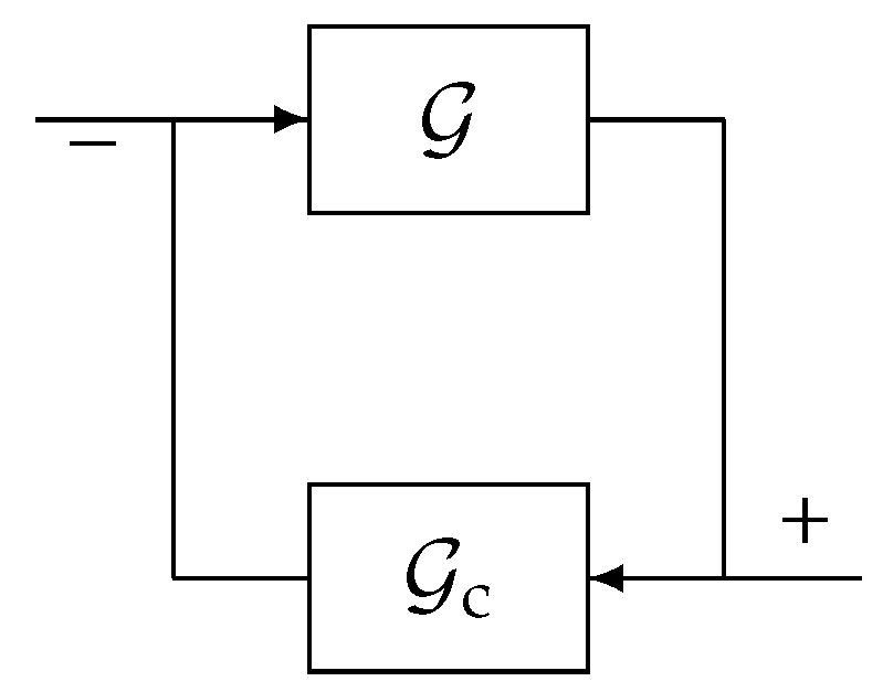
We begin by considering the negative feedback interconnection of the nonlinear dynamical system $\mathcal{G}$ given by (44) and (45), where $f\left(0\right)=0$ and $h\left(0\right)=0$, with the nonlinear feedback system ${\mathcal{G}}_{\mathrm{c}}$ given by

$$\begin{array}{ccc}\hfill {\dot{x}}_{\mathrm{c}}\left(t\right)& =& f_{\mathrm{c}}\left(x_{\mathrm{c}}\left(t\right)\right)+G_{\mathrm{c}}(u_{\mathrm{c}}\left(t\right),x_{\mathrm{c}}\left(t\right))u_{\mathrm{c}}\left(t\right),x_{\mathrm{c}}\left(0\right)=x_{\mathrm{c}0},t\ge 0,\hfill \end{array}$$

(66)

$$\begin{array}{ccc}\hfill y_{\mathrm{c}}\left(t\right)& =& h_{\mathrm{c}}(u_{\mathrm{c}}\left(t\right),x_{\mathrm{c}}\left(t\right))+J_{\mathrm{c}}(u_{\mathrm{c}}\left(t\right),x_{\mathrm{c}}\left(t\right))u_{\mathrm{c}}\left(t\right),\hfill \end{array}$$

(67)

where $x_{\mathrm{c}}\in {\mathbb{R}}^{n_{\mathrm{c}}}$, $u_{\mathrm{c}}\in {\mathbb{R}}^{m_{\mathrm{c}}}$, $y_{\mathrm{c}}\in {\mathbb{R}}^{l_{\mathrm{c}}}$, $f_{\mathrm{c}}:{\mathbb{R}}^{n_{\mathrm{c}}}\to {\mathbb{R}}^{n_{\mathrm{c}}}$ and satisfies $f_{\mathrm{c}}\left(0\right)=0$, $G_{\mathrm{c}}:{\mathbb{R}}^{m_{\mathrm{c}}}\times {\mathbb{R}}^{n_{\mathrm{c}}}\to {\mathbb{R}}^{n_{\mathrm{c}}\times m_{\mathrm{c}}}$, $h_{\mathrm{c}}:{\mathbb{R}}^{m_{\mathrm{c}}}\times {\mathbb{R}}^{n_{\mathrm{c}}}\to {\mathbb{R}}^{l_{\mathrm{c}}}$ and satisfies $h_{\mathrm{c}}(0,0)=0$, $J_{\mathrm{c}}:{\mathbb{R}}^{m_{\mathrm{c}}}\times {\mathbb{R}}^{n_{\mathrm{c}}}\to {\mathbb{R}}^{l_{\mathrm{c}}\times m_{\mathrm{c}}}$, $m_{\mathrm{c}}=l$, and $l_{\mathrm{c}}=m$. Note that for the negative feedback interconnection given by Figure 8, $u_{\mathrm{c}}=y$ and $y_{\mathrm{c}}=-u$. We assume that $f_{\mathrm{c}}(·)$, $G_{\mathrm{c}}(·,·)$, $h_{\mathrm{c}}(·,·)$, and $J_{\mathrm{c}}(·,·)$ are continuous mappings and the required properties for the existence of solutions in forward time, except possibly at the origin, of the negative feedback interconnection of $\mathcal{G}$ and ${\mathcal{G}}_{\mathrm{c}}$ are satisfied. Here, we also assume that the feedback interconnection of $\mathcal{G}$ and ${\mathcal{G}}_{\mathrm{c}}$ is well posed; that is, det$[I_m+J_{\mathrm{c}}(y,x_{\mathrm{c}})J\left(x\right)]\ne 0$ for all y, x, and $x_{\mathrm{c}}$.

The following results extend the results of [16,17] presenting sufficient conditions for Lyapunov stability, asymptotic stability, and finite-time stability to fixed-time stability of the feedback interconnection given in Figure 8.

Theorem 6. 

Consider the closed-loop system consisting of the nonlinear dynamical systems $\mathcal{G}$ given by (44) and (45), and ${\mathcal{G}}_{\mathrm{c}}$ given by (66) and (67) with input–output pairs $(u,y)$ and $(u_{\mathrm{c}},y_{\mathrm{c}})$, respectively, and with $u_{\mathrm{c}}=y$ and $y_{\mathrm{c}}=-u$. Assume that $\mathcal{G}$ and ${\mathcal{G}}_{\mathrm{c}}$ are zero-state observable and dissipative with respect to supply rates $r(u,y)$ and $r_{\mathrm{c}}(u_{\mathrm{c}},y_{\mathrm{c}})$, and with continuously differentiable positive definite, radially unbounded storage functions $V_{\mathrm{s}}(·)$ and $V_{\mathrm{sc}}(·)$, respectively, such that $V_{\mathrm{s}}\left(0\right)=0$ and $V_{\mathrm{sc}}\left(0\right)=0$. Furthermore, assume there exists a scalar $\sigma >0$ such that $r(u,y)+\sigma r_{\mathrm{c}}(u_{\mathrm{c}},y_{\mathrm{c}})\le 0$. Then the following statements hold:

(i)

The negative feedback interconnection of $\mathcal{G}$ and ${\mathcal{G}}_{\mathrm{c}}$ is Lyapunov stable.

(ii)

If ${\mathcal{G}}_{\mathrm{c}}$ is strongly dissipative or uniformly strongly dissipative with respect to supply rate $r_{\mathrm{c}}(u_{\mathrm{c}},y_{\mathrm{c}})$ and rank$[G_{\mathrm{c}}(u_{\mathrm{c}},0)]$$=m$, $u_{\mathrm{c}}\in {\mathbb{R}}^{m_{\mathrm{c}}}$, then the negative feedback interconnection of $\mathcal{G}$ and ${\mathcal{G}}_{\mathrm{c}}$ is globally asymptotically stable.

(iii)

If $\mathcal{G}$ and ${\mathcal{G}}_{\mathrm{c}}$ with either $x_0\ne 0$ or $x_{\mathrm{c}0}\ne 0$ are strongly dissipative with respect to supply rates $r(u,y)$ and $r_{\mathrm{c}}(u_{\mathrm{c}},y_{\mathrm{c}})$, respectively, then the negative feedback interconnection of $\mathcal{G}$ and ${\mathcal{G}}_{\mathrm{c}}$ is globally finite-time stable and there exists a continuous settling-time function $T:{\mathbb{R}}^n\times {\mathbb{R}}^{n_{\mathrm{c}}}\to [0,\infty )$ such that, for all $(x_0,x_{\mathrm{c}0})\in {\mathbb{R}}^n\times {\mathbb{R}}^{n_{\mathrm{c}}}$,

$$T(x_0,x_{\mathrm{c}0})\le {\displaystyle \frac{1}{\tilde{a}(1-\tilde{\alpha })}}{\left(V_{\mathrm{s}}\left(x_0\right)+\sigma V_{\mathrm{sc}}\left(x_{\mathrm{c}0}\right)\right)}^{1-\tilde{\alpha }},$$

(68)

where $\tilde{a}>0$ and $\tilde{\alpha }\in (0,1)$.

(iv)

If $\mathcal{G}$ and ${\mathcal{G}}_{\mathrm{c}}$ with either $x_0\ne 0$ or $x_{\mathrm{c}0}\ne 0$ are uniformly strongly dissipative with respect to supply rates $r(u,y)$ and $r_{\mathrm{c}}(u_{\mathrm{c}},y_{\mathrm{c}})$, respectively, then the negative feedback interconnection of $\mathcal{G}$ and ${\mathcal{G}}_{\mathrm{c}}$ is globally fixed-time stable and there exists a continuous settling-time function $T:{\mathbb{R}}^n\times {\mathbb{R}}^{n_{\mathrm{c}}}\to [0,\infty )$ such that, for all $(x_0,x_{\mathrm{c}0})\in {\mathbb{R}}^n\times {\mathbb{R}}^{n_{\mathrm{c}}}$,

$$T(x_0,x_{\mathrm{c}0})\le T_{max}={\displaystyle \frac{1}{(1-\tilde{\delta })\tilde{c}}}ln\left(1+{\displaystyle \frac{\tilde{c}}{\tilde{a}}}\right)+{\displaystyle \frac{1}{(\widehat{\theta }-1)\tilde{c}}}ln\left(1+{\displaystyle \frac{2^{\tilde{\theta }-1}\tilde{c}}{\tilde{b}}}\right),$$

(69)

where $\tilde{a}>0,\tilde{b}>0,\tilde{c}>0,\tilde{\delta }\in (0,1)$, $\tilde{\theta }>1$, and $\widehat{\theta }>1$.

(v)

If $\mathcal{G}$ is strongly dissipative and ${\mathcal{G}}_{\mathrm{c}}$ is uniformly strongly dissipative with respect to supply rates $r(u,y)$ and $r_{\mathrm{c}}(u_{\mathrm{c}},y_{\mathrm{c}})$, respectively, and $V_{\mathrm{s}}\left(x_0\right)+\sigma V_{\mathrm{sc}}\left(x_{\mathrm{c}0}\right)\le 1$, then the negative feedback interconnection of $\mathcal{G}$ and ${\mathcal{G}}_{\mathrm{c}}$ is fixed-time stable and there exists a continuous settling-time function $T:{\mathbb{R}}^n\times {\mathbb{R}}^{n_{\mathrm{c}}}\to [0,\infty )$ such that, for all $(x_0,x_{\mathrm{c}0})\in {\mathbb{R}}^n\times {\mathbb{R}}^{n_{\mathrm{c}}}$,

$$\begin{array}{cc}\hfill T(x_0,x_{\mathrm{c}0})\le T_{max}=& {\displaystyle \frac{1}{(1-\tilde{\delta })\tilde{c}}}ln\left[1+{\displaystyle \frac{\tilde{c}}{\tilde{a}}}{\left({\displaystyle \frac{2^{\tilde{\theta }-1}\tilde{a}}{\tilde{b}}}\right)}^{{\displaystyle \frac{1-\tilde{\delta }}{\tilde{\theta }-\tilde{\delta }}}}\right]\hfill \\ \hfill & +{\displaystyle \frac{1}{(\tilde{\theta }-1)\tilde{c}}}ln\left[1+{\displaystyle \frac{\tilde{c}}{\tilde{b}}}{\left({\displaystyle \frac{\tilde{b}}{2^{\tilde{\theta }-1}\tilde{a}}}\right)}^{{\displaystyle \frac{\tilde{\theta }-1}{\tilde{\theta }-\tilde{\delta }}}}\right],\hfill \end{array}$$

where $\tilde{a}>0,\tilde{b}>0,\tilde{c}>0,\tilde{\delta }\in (0,1)$, and $\tilde{\theta }>1$.

Proof. 

The proofs of (i)–($iii$) are given in Theorem 6.1 of [16] and Theorem 4.1 of [17] using the Lyapunov function candidate $V(x,x_{\mathrm{c}})=V_{\mathrm{s}}\left(x\right)+\sigma V_{\mathrm{sc}}\left(x_{\mathrm{c}}\right)$, and hence, are omitted.

To show ($iv$), note that since $\mathcal{G}$ and ${\mathcal{G}}_{\mathrm{c}}$ are uniformly strongly dissipative with respect to the supply rates $r(u,y)$ and $r_{\mathrm{c}}(u_{\mathrm{c}},y_{\mathrm{c}})$, respectively, it follows from Definition 3 and Remark 4 that there exist constants $a,a_{\mathrm{c}},b,b_{\mathrm{c}},c,c_{\mathrm{c}},\delta ,{\delta }_{\mathrm{c}},\theta ,{\theta }_{\mathrm{c}},k,k_{\mathrm{c}}>0$ such that $\delta k<1$, $\theta k>1$, ${\delta }_{\mathrm{c}}{k}_{\mathrm{c}}<1$, ${\theta }_{\mathrm{c}}{k}_{\mathrm{c}}>1$, and

$$\begin{array}{cc}\hfill {\dot{V}}_{\mathrm{s}}(x,u)+{[a{V}_{\mathrm{s}}^{\delta }\left(x\right)+b{V}_{\mathrm{s}}^{\theta }\left(x\right)]}^k+c{V}_{\mathrm{s}}\left(x\right)& \le r(u,y),(x,u)\in {\mathbb{R}}^n\times {\mathbb{R}}^m,\hfill \end{array}$$

(70)

$$\begin{array}{cc}\hfill {\dot{V}}_{\mathrm{sc}}(x_{\mathrm{c}},u_{\mathrm{c}})+{[a_{\mathrm{c}}{V}_{\mathrm{sc}}^{{\delta }_{\mathrm{c}}}\left(x_{\mathrm{c}}\right)+b_{\mathrm{c}}{V}_{\mathrm{sc}}^{{\theta }_{\mathrm{c}}}\left(x_{\mathrm{c}}\right)]}^{k_{\mathrm{c}}}+c_{\mathrm{c}}{V}_{\mathrm{sc}}\left(x_{\mathrm{c}}\right)& \le r_{\mathrm{c}}(u_{\mathrm{c}},y_{\mathrm{c}}),(x_{\mathrm{c}},u_{\mathrm{c}})\in {\mathbb{R}}^{n_{\mathrm{c}}}\times {\mathbb{R}}^{m_{\mathrm{c}}}.\hfill \end{array}$$

(71)

Now, consider the Lyapunov function candidate $V(x,x_{\mathrm{c}})=V_{\mathrm{s}}\left(x\right)+\sigma V_{\mathrm{sc}}\left(x_{\mathrm{c}}\right)$ and note that the total derivative of V along the closed-loop system state trajectories through $(x,x_{\mathrm{c}})\in {\mathbb{R}}^n\times {\mathbb{R}}^{n_{\mathrm{c}}}$ at $t=0$ is given by

$$\begin{array}{cc}\hfill \dot{V}(x,x_{\mathrm{c}})& =\dot{V_{\mathrm{s}}}\left(x\right)+\sigma {\dot{V}}_{\mathrm{sc}}\left(x_{\mathrm{c}}\right)\hfill \\ \hfill & \le -{[a{V}_{\mathrm{s}}^{\delta }\left(x\right)+b{V}_{\mathrm{s}}^{\theta }\left(x\right)]}^k-c{V}_{\mathrm{s}}\left(x\right)-\sigma {[a_{\mathrm{c}}{V}_{\mathrm{sc}}^{{\delta }_{\mathrm{c}}}\left(x_{\mathrm{c}}\right)+b_{\mathrm{c}}{V}_{\mathrm{sc}}^{{\theta }_{\mathrm{c}}}\left(x_{\mathrm{c}}\right)]}^{k_{\mathrm{c}}}\hfill \\ \hfill & -\sigma c_{\mathrm{c}}{V}_{\mathrm{sc}}\left(x_{\mathrm{c}}\right)+r(u,y)+\sigma r_{\mathrm{c}}(u_{\mathrm{c}},y_{\mathrm{c}})\hfill \\ \hfill & \le -{[a{V}_{\mathrm{s}}^{\delta }\left(x\right)+b{V}_{\mathrm{s}}^{\theta }\left(x\right)]}^k-c{V}_{\mathrm{s}}\left(x\right)-\sigma {[a_{\mathrm{c}}{V}_{\mathrm{sc}}^{{\delta }_{\mathrm{c}}}\left(x_{\mathrm{c}}\right)+b_{\mathrm{c}}{V}_{\mathrm{sc}}^{{\theta }_{\mathrm{c}}}\left(x_{\mathrm{c}}\right)]}^{k_{\mathrm{c}}}-\sigma c_{\mathrm{c}}{V}_{\mathrm{sc}}\left(x_{\mathrm{c}}\right).\hfill \end{array}$$

(72)

Next, using the fact that, for all $z_1$, $z_2$, and $\nu \in \mathbb{R}$ (see ([27], pp. 50–57)),

$$\begin{array}{cc}\hfill (|z_1|+|z_2{|)}^{\nu }& \ge {\displaystyle \frac{1}{2^{1-\nu }}}(|z_1{|}^{\nu }+|z_2{|}^{\nu }),\nu <1,\hfill \end{array}$$

(73)

$$\begin{array}{cc}\hfill (|z_1|+|z_2{|)}^{\nu }& \ge |z_1{|}^{\nu }+{|z_2|}^{\nu }\nu \ge 1,\hfill \end{array}$$

(74)

(72) gives

$$\begin{array}{cc}\hfill \dot{V}(x,x_{\mathrm{c}})\le & -p[a^k{V}_{\mathrm{s}}^{\delta k}\left(x\right)+b^k{V}_{\mathrm{s}}^{\theta k}\left(x\right)]-c{V}_{\mathrm{s}}\left(x\right)-q[\sigma a_{\mathrm{c}}^{k_{\mathrm{c}}}{V}_{\mathrm{sc}}^{{\delta }_{\mathrm{c}}{k}_{\mathrm{c}}}\left(x_{\mathrm{c}}\right)+\sigma b_{\mathrm{c}}^{k_{\mathrm{c}}}{V}_{\mathrm{sc}}^{{\theta }_{\mathrm{c}}{k}_{\mathrm{c}}}\left(x_{\mathrm{c}}\right)]\hfill \\ \hfill & -\sigma c_{\mathrm{c}}{V}_{\mathrm{sc}}\left(x_{\mathrm{c}}\right),(x,x_{\mathrm{c}})\in {\mathbb{R}}^n\times {\mathbb{R}}^{n_{\mathrm{c}}},\hfill \end{array}$$

(75)

where

$$(p,q)=\left\{\begin{array}{cc}\left(1,1\right),\hfill & k\ge 1,k_{\mathrm{c}}\ge 1,\hfill \\ \left({\displaystyle \frac{1}{2^{1-k}}},1\right),\hfill & k\le 1,k_{\mathrm{c}}\ge 1,\hfill \\ \left(1,{\displaystyle \frac{1}{2^{1-k_{\mathrm{c}}}}}\right),\hfill & k\ge 1,k_{\mathrm{c}}\le 1,\hfill \\ \left({\displaystyle \frac{1}{2^{1-k}}},{\displaystyle \frac{1}{2^{1-k_{\mathrm{c}}}}}\right),\hfill & k\le 1,k_{\mathrm{c}}\le 1.\hfill \end{array}\right.$$

(76)

Here, we show the analysis for the case where $(p,q)=(1,1)$ (i.e., $k\ge 1$ and $k_{\mathrm{c}}\ge 1$). The proof for the other pairs of $(p,q)$ in (76) is analogous.

Next, note that (75) implies that, for all $t\ge 0$, $V(x\left(t\right),x_{\mathrm{c}}\left(t\right))\le V(x_0,x_{\mathrm{c}0})$. Define $\tilde{c}\triangleq \min \{c,c_{\mathrm{c}}\}$, $\tilde{\delta }\triangleq max\{\delta k,{\delta }_{\mathrm{c}}{k}_{\mathrm{c}}\}<1$, $\tilde{\theta }\triangleq max\{\theta k,{\theta }_{\mathrm{c}}{k}_{\mathrm{c}}\}>1$, $\widehat{\delta }\triangleq min\{\delta k,{\delta }_{\mathrm{c}}{k}_{\mathrm{c}}\}<1$, $\widehat{\theta }\triangleq min\{\theta k,{\theta }_{\mathrm{c}}{k}_{\mathrm{c}}\}>1$, $\tilde{a}\triangleq min\{a^k,{\sigma }^{1-{\delta }_{\mathrm{c}}{k}_{\mathrm{c}}}{a}_{\mathrm{c}}^{k_{\mathrm{c}}}\}$, and $\tilde{b}\triangleq min\{b^k,{\sigma }^{1-{\theta }_{\mathrm{c}}{k}_{\mathrm{c}}}{b}_{\mathrm{c}}^{k_{\mathrm{c}}}\}$, and consider the following two cases: a) $V(x_0,x_{\mathrm{c}0})\le 1$ and b) $V(x_0,x_{\mathrm{c}0})>1$. For $V(x_0,x_{\mathrm{c}0})\le 1$, note that $V(x\left(t\right),x_{\mathrm{c}}\left(t\right))\le 1$, $t\ge 0$, and consequently, $V_{\mathrm{s}}\left(x\left(t\right)\right)\le 1$, $t\ge 0$, and $\sigma V_{\mathrm{sc}}\left(x_{\mathrm{c}}\left(t\right)\right)\le 1$, $t\ge 0$. Hence, on the closed-loop system trajectories (75) becomes

$$\begin{array}{cc}\hfill \dot{V}(x\left(t\right),x_{\mathrm{c}}\left(t\right))& \le -a^k{V}_{\mathrm{s}}^{\delta k}\left(x\left(t\right)\right)-b^k{V}_{\mathrm{s}}^{\theta k}\left(x\left(t\right)\right)-\sigma a_{\mathrm{c}}^{k_{\mathrm{c}}}{V}_{\mathrm{sc}}^{{\delta }_{\mathrm{c}}{k}_{\mathrm{c}}}\left(x_{\mathrm{c}}\left(t\right)\right)-\sigma b_{\mathrm{c}}^{k_{\mathrm{c}}}{V}_{\mathrm{sc}}^{{\theta }_{\mathrm{c}}{k}_{\mathrm{c}}}\left(x_{\mathrm{c}}\left(t\right)\right)\hfill \\ \hfill & -c{V}_{\mathrm{s}}\left(x\left(t\right)\right)-c_{\mathrm{c}}\sigma V_{\mathrm{sc}}\left(x_{\mathrm{c}}\left(t\right)\right)\hfill \\ \hfill & \le -a^k{V}_{\mathrm{s}}^{\delta k}\left(x\left(t\right)\right)-b^k{V}_{\mathrm{s}}^{\theta k}\left(x\left(t\right)\right)-\sigma a_{\mathrm{c}}^{k_{\mathrm{c}}}{V}_{\mathrm{sc}}^{{\delta }_{\mathrm{c}}{k}_{\mathrm{c}}}\left(x_{\mathrm{c}}\left(t\right)\right)-\sigma b_{\mathrm{c}}^{k_{\mathrm{c}}}{V}_{\mathrm{sc}}^{{\theta }_{\mathrm{c}}{k}_{\mathrm{c}}}\left(x_{\mathrm{c}}\left(t\right)\right)\hfill \\ \hfill & -\tilde{c}V(x\left(t\right),x_{\mathrm{c}}\left(t\right))\hfill \\ \hfill & \le -a^k{V}_{\mathrm{s}}^{\tilde{\delta }}\left(x\left(t\right)\right)-b^k{V}_{\mathrm{s}}^{\tilde{\theta }}\left(x\left(t\right)\right)-{\sigma }^{1-{\delta }_{\mathrm{c}}{k}_{\mathrm{c}}}{a}_{\mathrm{c}}^{k_{\mathrm{c}}}{\left(\sigma V_{\mathrm{sc}}\left(x_{\mathrm{c}}\left(t\right)\right)\right)}^{\tilde{\delta }}\hfill \\ \hfill & -{\sigma }^{1-{\theta }_{\mathrm{c}}{k}_{\mathrm{c}}}{b}_{\mathrm{c}}^{k_{\mathrm{c}}}{\left(\sigma V_{\mathrm{sc}}\left(x_{\mathrm{c}}\left(t\right)\right)\right)}^{\tilde{\theta }}-\tilde{c}V(x\left(t\right),x_{\mathrm{c}}\left(t\right))\hfill \\ \hfill & \le -\tilde{a}(V_{\mathrm{s}}^{\tilde{\delta }}\left(x\left(t\right)\right)+{\left(\sigma V_{\mathrm{sc}}\left(x_{\mathrm{c}}\left(t\right)\right)\right)}^{\tilde{\delta }})-\tilde{b}(V_{\mathrm{s}}^{\tilde{\theta }}\left(x\left(t\right)\right)+{\left(\sigma V_{\mathrm{sc}}\left(x_{\mathrm{c}}\left(t\right)\right)\right)}^{\tilde{\theta }})\hfill \\ \hfill & -\tilde{c}V(x\left(t\right),x_{\mathrm{c}}\left(t\right))\hfill \\ \hfill & \le -\tilde{a}{(V_{\mathrm{s}}\left(x\left(t\right)\right)+\sigma V_{\mathrm{sc}}\left(x_{\mathrm{c}}\left(t\right)\right))}^{\tilde{\delta }}-{\displaystyle \frac{\tilde{b}}{2^{\tilde{\theta }-1}}}{(V_{\mathrm{s}}\left(x\left(t\right)\right)+\sigma V_{\mathrm{sc}}\left(x_{\mathrm{c}}\left(t\right)\right))}^{\tilde{\theta }}\hfill \\ \hfill & -\tilde{c}V(x\left(t\right),x_{\mathrm{c}}\left(t\right))\hfill \\ \hfill & =-\tilde{a}{V}^{\tilde{\delta }}(x\left(t\right),x_{\mathrm{c}}\left(t\right))-{\displaystyle \frac{\tilde{b}}{2^{\tilde{\theta }-1}}}{V}^{\tilde{\theta }}(x\left(t\right),x_{\mathrm{c}}\left(t\right))-\tilde{c}V(x\left(t\right),x_{\mathrm{c}}\left(t\right)),t\ge 0,\hfill \end{array}$$

(77)

where the third inequality in (77) follows from the fact that for $z\in [0,1]$, $z^q\ge z^p$ for all $p\ge q$, and the fifth inequality in (77) follows from the fact that (see ([27], pp. 50–57))

$$\begin{array}{cc}\hfill (|z_1|+|z_2{|)}^k& \le |z_1{|}^k+{|z_2|}^k,k<1,\hfill \end{array}$$

(78)

$$\begin{array}{cc}\hfill (|z_1|+|z_2{|)}^k& \le 2^{k-1}(|z_1{|}^k+|z_2{|}^k),k>1.\hfill \end{array}$$

(79)

Next, for $V(x_0,x_{\mathrm{c}0})>1$, note that since $V_{\mathrm{s}}\left(x\right)$ and $V_{\mathrm{sc}}\left(x_{\mathrm{c}}\right)$ are positive definite and, for all $t\ge 0$, $V(x\left(t\right),x_{\mathrm{c}}\left(t\right))$ is nonincreasing, and hence,

$${\displaystyle \frac{V_{\mathrm{s}}\left(x\left(t\right)\right)}{V(x\left(t\right),x_{\mathrm{c}}\left(t\right))}}\le 1\mathrm{and}{\displaystyle \frac{\sigma V_{\mathrm{sc}}\left(x_{\mathrm{c}}\left(t\right)\right)}{V(x\left(t\right),x_{\mathrm{c}}\left(t\right))}}\le 1,$$

(80)

for all $t\ge 0$. Hence, using (80), (75) gives

$$\begin{array}{cc}\hfill \dot{V}(x\left(t\right),x_{\mathrm{c}}\left(t\right))& \le -a^k{V}_{\mathrm{s}}^{\delta k}\left(x\left(t\right)\right)-b^k{V}_{\mathrm{s}}^{\theta k}\left(x\left(t\right)\right)-\sigma a_{\mathrm{c}}^{k_{\mathrm{c}}}{V}_{\mathrm{sc}}^{{\delta }_{\mathrm{c}}{k}_{\mathrm{c}}}\left(x_{\mathrm{c}}\left(t\right)\right)-\sigma b_{\mathrm{c}}^{k_{\mathrm{c}}}{V}_{\mathrm{sc}}^{{\theta }_{\mathrm{c}}{k}_{\mathrm{c}}}\left(x_{\mathrm{c}}\left(t\right)\right)\hfill \\ \hfill & -c{V}_{\mathrm{s}}\left(x\left(t\right)\right)-c_{\mathrm{c}}\sigma V_{\mathrm{sc}}\left(x_{\mathrm{c}}\left(t\right)\right)\hfill \\ \hfill & \le -a^k{V}_{\mathrm{s}}^{\delta k}\left(x\left(t\right)\right)-b^k{V}_{\mathrm{s}}^{\theta k}\left(x\left(t\right)\right)-\sigma a_{\mathrm{c}}^{k_{\mathrm{c}}}{V}_{\mathrm{sc}}^{{\delta }_{\mathrm{c}}{k}_{\mathrm{c}}}\left(x_{\mathrm{c}}\left(t\right)\right)-\sigma b_{\mathrm{c}}^{k_{\mathrm{c}}}{V}_{\mathrm{sc}}^{{\theta }_{\mathrm{c}}{k}_{\mathrm{c}}}\left(x_{\mathrm{c}}\left(t\right)\right)\hfill \\ \hfill & -\tilde{c}V(x\left(t\right),x_{\mathrm{c}}\left(t\right))\hfill \\ \hfill & =-a^k{V}^{\delta k}(x\left(t\right),x_{\mathrm{c}}\left(t\right)){\left({\displaystyle \frac{V_{\mathrm{s}}\left(x\left(t\right)\right)}{V(x\left(t\right),x_{\mathrm{c}}\left(t\right))}}\right)}^{\delta k}-b^k{V}^{\theta k}(x\left(t\right),x_{\mathrm{c}}\left(t\right))\hfill \\ \hfill & ·{\left({\displaystyle \frac{V_{\mathrm{s}}\left(x\left(t\right)\right)}{V(x\left(t\right),x_{\mathrm{c}}\left(t\right))}}\right)}^{\theta k}-{\sigma }^{1-{\delta }_{\mathrm{c}}{k}_{\mathrm{c}}}{a}_{\mathrm{c}}^{k_{\mathrm{c}}}{V}^{{\delta }_{\mathrm{c}}{k}_{\mathrm{c}}}(x\left(t\right),x_{\mathrm{c}}\left(t\right)){\left({\displaystyle \frac{\sigma V_{\mathrm{sc}}\left(x_{\mathrm{c}}\left(t\right)\right)}{V(x\left(t\right),x_{\mathrm{c}}\left(t\right))}}\right)}^{{\delta }_{\mathrm{c}}{k}_{\mathrm{c}}}\hfill \\ \hfill & -{\sigma }^{1-{\theta }_{\mathrm{c}}{k}_{\mathrm{c}}}{b}_{\mathrm{c}}^{k_{\mathrm{c}}}{V}^{{\theta }_{\mathrm{c}}{k}_{\mathrm{c}}}(x\left(t\right),x_{\mathrm{c}}\left(t\right)){\left({\displaystyle \frac{\sigma V_{\mathrm{sc}}\left(x_{\mathrm{c}}\left(t\right)\right)}{V(x\left(t\right),x_{\mathrm{c}}\left(t\right))}}\right)}^{{\theta }_{\mathrm{c}}{k}_{\mathrm{c}}}-\tilde{c}V(x\left(t\right),x_{\mathrm{c}}\left(t\right))\hfill \\ \hfill & \le -a^k{V}^{\delta k}(x\left(t\right),x_{\mathrm{c}}\left(t\right)){\left({\displaystyle \frac{V_{\mathrm{s}}\left(x\left(t\right)\right)}{V(x\left(t\right),x_{\mathrm{c}}\left(t\right))}}\right)}^{\tilde{\delta }}-b^k{V}^{\theta k}(x\left(t\right),x_{\mathrm{c}}\left(t\right))\hfill \\ \hfill & ·{\left({\displaystyle \frac{V_{\mathrm{s}}\left(x\left(t\right)\right)}{V(x\left(t\right),x_{\mathrm{c}}\left(t\right))}}\right)}^{\tilde{\theta }}-{\sigma }^{1-{\delta }_{\mathrm{c}}{k}_{\mathrm{c}}}{a}_{\mathrm{c}}^{k_{\mathrm{c}}}{V}^{{\delta }_{\mathrm{c}}{k}_{\mathrm{c}}}(x\left(t\right),x_{\mathrm{c}}\left(t\right)){\left({\displaystyle \frac{\sigma V_{\mathrm{sc}}\left(x_{\mathrm{c}}\left(t\right)\right)}{V(x\left(t\right),x_{\mathrm{c}}\left(t\right))}}\right)}^{\tilde{\delta }}\hfill \\ \hfill & -{\sigma }^{1-{\theta }_{\mathrm{c}}{k}_{\mathrm{c}}}{b}_{\mathrm{c}}^{k_{\mathrm{c}}}{V}^{{\theta }_{\mathrm{c}}{k}_{\mathrm{c}}}(x\left(t\right),x_{\mathrm{c}}\left(t\right)){\left({\displaystyle \frac{\sigma V_{\mathrm{sc}}\left(x_{\mathrm{c}}\left(t\right)\right)}{V(x\left(t\right),x_{\mathrm{c}}\left(t\right))}}\right)}^{\tilde{\theta }}-\tilde{c}V(x\left(t\right),x_{\mathrm{c}}\left(t\right))\hfill \\ \hfill & \le -a^k{V}^{\widehat{\delta }}(x\left(t\right),x_{\mathrm{c}}\left(t\right)){\left({\displaystyle \frac{V_{\mathrm{s}}\left(x\left(t\right)\right)}{V(x\left(t\right),x_{\mathrm{c}}\left(t\right))}}\right)}^{\tilde{\delta }}-b^k{V}^{\widehat{\theta }}(x\left(t\right),x_{\mathrm{c}}\left(t\right))\hfill \\ \hfill & ·{\left({\displaystyle \frac{V_{\mathrm{s}}\left(x\left(t\right)\right)}{V(x\left(t\right),x_{\mathrm{c}}\left(t\right))}}\right)}^{\tilde{\theta }}-{\sigma }^{1-{\delta }_{\mathrm{c}}{k}_{\mathrm{c}}}{a}_{\mathrm{c}}^{k_{\mathrm{c}}}{V}^{\widehat{\delta }}(x\left(t\right),x_{\mathrm{c}}\left(t\right)){\left({\displaystyle \frac{\sigma V_{\mathrm{sc}}\left(x_{\mathrm{c}}\left(t\right)\right)}{V(x\left(t\right),x_{\mathrm{c}}\left(t\right))}}\right)}^{\tilde{\delta }}\hfill \\ \hfill & -{\sigma }^{1-{\theta }_{\mathrm{c}}{k}_{\mathrm{c}}}{b}_{\mathrm{c}}^{k_{\mathrm{c}}}{V}^{\widehat{\theta }}(x\left(t\right),x_{\mathrm{c}}\left(t\right)){\left({\displaystyle \frac{\sigma V_{\mathrm{sc}}\left(x_{\mathrm{c}}\left(t\right)\right)}{V(x\left(t\right),x_{\mathrm{c}}\left(t\right))}}\right)}^{\tilde{\theta }}-\tilde{c}V(x\left(t\right),x_{\mathrm{c}}\left(t\right))\hfill \\ \hfill & \le -\tilde{a}{V}^{\widehat{\delta }-\tilde{\delta }}(x\left(t\right),x_{\mathrm{c}}\left(t\right))(V_{\mathrm{s}}^{\tilde{\delta }}\left(x\left(t\right)\right)+{\left(\sigma V_{\mathrm{sc}}\left(x_{\mathrm{c}}\left(t\right)\right)\right)}^{\tilde{\delta }})-\tilde{b}{V}^{\widehat{\theta }-\tilde{\theta }}(x\left(t\right),x_{\mathrm{c}}\left(t\right))\hfill \\ \hfill & ·(V_{\mathrm{s}}^{\tilde{\theta }}\left(x\left(t\right)\right)+{\left(\sigma V_{\mathrm{sc}}\left(x_{\mathrm{c}}\left(t\right)\right)\right)}^{\tilde{\theta }})-\tilde{c}V(x\left(t\right),x_{\mathrm{c}}\left(t\right)),t\ge 0,\hfill \end{array}$$

(81)

where the third inequality in (81) follows from the fact that, for $z\in [0,1]$, $z^q\ge z^p$ for all $p\ge q$.

Finally, using (78) and (79), it follows from (81) that

$$\begin{array}{cc}\hfill \dot{V}(x\left(t\right),x_{\mathrm{c}}\left(t\right))& \le -\tilde{a}{V}^{\widehat{\delta }-\tilde{\delta }}(x\left(t\right),x_{\mathrm{c}}\left(t\right)){(V_{\mathrm{s}}\left(x\left(t\right)\right)+\sigma V_{\mathrm{sc}}\left(x_{\mathrm{c}}\left(t\right)\right))}^{\tilde{\delta }}\hfill \\ \hfill & -{\displaystyle \frac{\tilde{b}}{2^{\tilde{\theta }-1}}}{V}^{\widehat{\theta }-\tilde{\theta }}(x\left(t\right),x_{\mathrm{c}}\left(t\right)){(V_{\mathrm{s}}\left(x\right)+\sigma V_{\mathrm{sc}}\left(x_{\mathrm{c}}\left(t\right)\right))}^{\tilde{\theta }}-\tilde{c}V(x\left(t\right),x_{\mathrm{c}}\left(t\right))\hfill \\ \hfill & \le -\tilde{a}{V}^{\widehat{\delta }-\tilde{\delta }}(x\left(t\right),x_{\mathrm{c}}\left(t\right))V^{\tilde{\delta }}(x\left(t\right),x_{\mathrm{c}}\left(t\right))\hfill \\ \hfill & -{\displaystyle \frac{\tilde{b}}{2^{\tilde{\theta }-1}}}{V}^{\widehat{\theta }-\tilde{\theta }}(x\left(t\right),x_{\mathrm{c}}\left(t\right))V^{\tilde{\theta }}(x\left(t\right),x_{\mathrm{c}}\left(t\right))-\tilde{c}V(x\left(t\right),x_{\mathrm{c}}\left(t\right))\hfill \\ \hfill & =-\tilde{a}{V}^{\widehat{\delta }}(x\left(t\right),x_{\mathrm{c}}\left(t\right))-{\displaystyle \frac{\tilde{b}}{2^{\tilde{\theta }-1}}}{V}^{\widehat{\theta }}(x\left(t\right),x_{\mathrm{c}}\left(t\right))-\tilde{c}V(x\left(t\right),x_{\mathrm{c}}\left(t\right)),t\ge 0.\hfill \end{array}$$

(82)

Hence, for $V(x,x_{\mathrm{c}})\le 1$ and $V(x,x_{\mathrm{c}})>1$, the Lyapunov derivatives on the closed-loop system trajectories given by (77) and (82), respectively, take the form given in (38). Thus, (77) proves fixed-time stability of the negative feedback interconnection of $\mathcal{G}$ and ${\mathcal{G}}_{\mathrm{c}}$ in the region ${\mathcal{D}}_1=\{(x,x_{\mathrm{c}}):V(x,x_{\mathrm{c}})\le 1$}, whereas (82) proves fixed-time convergence to the region ${\mathcal{D}}_1$. Thus, it follows that the negative feedback interconnection of $\mathcal{G}$ and ${\mathcal{G}}_{\mathrm{c}}$ is fixed-time stable and $(x\left(t\right),x_{\mathrm{c}}\left(t\right))=0,t\ge T(x_0,x_{\mathrm{c}0})$, where

$$T(x_0,x_{\mathrm{c}0})\le T_{max}={\displaystyle \frac{1}{(1-\tilde{\delta })\tilde{c}}}ln\left(1+{\displaystyle \frac{\tilde{c}}{\tilde{a}}}\right)+{\displaystyle \frac{1}{(\widehat{\theta }-1)\tilde{c}}}ln\left(1+{\displaystyle \frac{2^{\tilde{\theta }-1}\tilde{c}}{\tilde{b}}}\right),$$

(83)

is a continuous settling-time function on ${\mathbb{R}}^n\times {\mathbb{R}}^{n_{\mathrm{c}}}$ and where (83) is the sum of the time the closed-loop system takes to converge to the region ${\mathcal{D}}_1$ and the time it takes the closed-loop system to reach origin from $\partial {\mathcal{D}}_1$.

Finally, to show (v), note that since $\mathcal{G}$ is strongly dissipative and ${\mathcal{G}}_{\mathrm{c}}$ is uniformly strongly dissipative with respect to the supply rates $r(u,y)$ and $r_{\mathrm{c}}(u_{\mathrm{c}},y_{\mathrm{c}})$, respectively, it follows from Definition 3 and Remark 4 that there exist constants $a,a_{\mathrm{c}},b_{\mathrm{c}},c_{\mathrm{c}},\delta ,{\delta }_{\mathrm{c}},{\theta }_{\mathrm{c}},k$, $k_{\mathrm{c}}>0$ such that $\delta k<1$, ${\delta }_{\mathrm{c}}{k}_{\mathrm{c}}<1$, ${\theta }_{\mathrm{c}}{k}_{\mathrm{c}}>1$, and

$$\begin{array}{cc}\hfill {\dot{V}}_{\mathrm{s}}(x,u)+a^k{V}_{\mathrm{s}}^{\delta k}\left(x\right)& \le r(u,y),(x,u)\in {\mathbb{R}}^n\times {\mathbb{R}}^m,\hfill \end{array}$$

(84)

$$\begin{array}{cc}\hfill {\dot{V}}_{\mathrm{sc}}(x_{\mathrm{c}},u_{\mathrm{c}})+{[a_{\mathrm{c}}{V}_{\mathrm{sc}}^{{\delta }_{\mathrm{c}}}\left(x_{\mathrm{c}}\right)+b_{\mathrm{c}}{V}_{\mathrm{sc}}^{{\theta }_{\mathrm{c}}}\left(x_{\mathrm{c}}\right)]}^{k_{\mathrm{c}}}+c_{\mathrm{c}}{V}_{\mathrm{sc}}\left(x_{\mathrm{c}}\right)& \le r_{\mathrm{c}}(u_{\mathrm{c}},y_{\mathrm{c}}),(x_{\mathrm{c}},u_{\mathrm{c}})\in {\mathbb{R}}^{n_{\mathrm{c}}}\times {\mathbb{R}}^{m_{\mathrm{c}}}.\hfill \end{array}$$

(85)

Now, using the Lyapunov function candidate $V(x,x_{\mathrm{c}})=V_{\mathrm{s}}\left(x\right)+\sigma V_{\mathrm{sc}}\left(x_{\mathrm{c}}\right)$ it follows that the Lyapunov derivative along the closed-loop system trajectories is given by

$$\begin{array}{cc}\hfill \dot{V}(x\left(t\right),x_{\mathrm{c}}\left(t\right))& \le \dot{V}\left(x\left(t\right)\right)+\sigma {\dot{V}}_{\mathrm{sc}}\left(x_{\mathrm{c}}\left(t\right)\right)\hfill \\ \hfill & \le -a^k{V}_{\mathrm{s}}^{\delta k}\left(x\left(t\right)\right)-\sigma {[a_{\mathrm{c}}{V}_{\mathrm{sc}}^{{\delta }_{\mathrm{c}}}\left(x_{\mathrm{c}}\left(t\right)\right)+b_{\mathrm{c}}{V}_{\mathrm{sc}}^{{\theta }_{\mathrm{c}}}\left(x_{\mathrm{c}}\left(t\right)\right)]}^{k_{\mathrm{c}}}-\sigma c_{\mathrm{c}}{V}_{\mathrm{sc}}\left(x_{\mathrm{c}}\left(t\right)\right)\hfill \\ \hfill & +r(u,y)+\sigma r_{\mathrm{c}}(u_{\mathrm{c}},y_{\mathrm{c}})\hfill \\ \hfill & \le -a^k{V}_{\mathrm{s}}^{\delta k}\left(x\left(t\right)\right)-\sigma {[a_{\mathrm{c}}{V}_{\mathrm{sc}}^{{\delta }_{\mathrm{c}}}\left(x_{\mathrm{c}}\left(t\right)\right)+b_{\mathrm{c}}{V}_{\mathrm{sc}}^{{\theta }_{\mathrm{c}}}\left(x_{\mathrm{c}}\left(t\right)\right)]}^{k_{\mathrm{c}}}-\sigma c_{\mathrm{c}}{V}_{\mathrm{sc}}\left(x_{\mathrm{c}}\left(t\right)\right)\hfill \\ \hfill & \le -a^k{V}_{\mathrm{s}}^{\delta k}\left(x\left(t\right)\right)-\sigma a_{\mathrm{c}}^{k_{\mathrm{c}}}{V}_{\mathrm{sc}}^{{\delta }_{\mathrm{c}}{k}_{\mathrm{c}}}\left(x_{\mathrm{c}}\left(t\right)\right)-\sigma b_{\mathrm{c}}^{k_{\mathrm{c}}}{V}_{\mathrm{sc}}^{{\theta }_{\mathrm{c}}{k}_{\mathrm{c}}}\left(x_{\mathrm{c}}\left(t\right)\right)-\sigma c_{\mathrm{c}}{V}_{\mathrm{sc}}\left(x_{\mathrm{c}}\left(t\right)\right)\hfill \\ \hfill & =-{\displaystyle \frac{a^k}{3}}{V}_{\mathrm{s}}^{\delta k}\left(x\left(t\right)\right)-{\displaystyle \frac{a^k}{3}}{V}_{\mathrm{s}}^{\delta k}\left(x\left(t\right)\right)-{\displaystyle \frac{a^k}{3}}{V}_{\mathrm{s}}^{\delta k}\left(x\left(t\right)\right)-\sigma a_{\mathrm{c}}^{k_{\mathrm{c}}}{V}_{\mathrm{sc}}^{{\delta }_{\mathrm{c}}{k}_{\mathrm{c}}}\left(x_{\mathrm{c}}\left(t\right)\right)\hfill \\ \hfill & -\sigma b_{\mathrm{c}}^{k_{\mathrm{c}}}{V}_{\mathrm{sc}}^{{\theta }_{\mathrm{c}}{k}_{\mathrm{c}}}\left(x_{\mathrm{c}}\left(t\right)\right)-\sigma c_{\mathrm{c}}{V}_{\mathrm{sc}}\left(x_{\mathrm{c}}\left(t\right)\right),t\ge 0.\hfill \end{array}$$

(86)

Note that since $V(x\left(t\right),x_{\mathrm{c}}\left(t\right))$, $t\ge 0$, is nonincreasing, for $V(x_0,x_{\mathrm{c}0})\le 1$, $V(x\left(t\right),x_{\mathrm{c}}\left(t\right))\le 1$, $t\ge 0$, and consequently $V_{\mathrm{s}}\left(x\left(t\right)\right)\le 1$, $t\ge 0$, and $\sigma V_{\mathrm{sc}}\left(x_{\mathrm{c}}\left(t\right)\right)\le 1$, $t\ge 0$. Hence, since, for every $t\ge 0$, $V_{\mathrm{s}}\left(x\left(t\right)\right)\le 1$, it follows that

$$V_{\mathrm{s}}^{\theta k}\left(x\left(t\right)\right)\le V_{\mathrm{s}}\left(x\left(t\right)\right)\le V_{\mathrm{s}}^{\delta k}\left(x\left(t\right)\right)\le 1,t\ge 0,$$

where $\theta k\ge 1$.

Next, define $\tilde{a}\triangleq min\{{\displaystyle \frac{a^k}{3}},{\sigma }^{1-{\delta }_{\mathrm{c}}{k}_{\mathrm{c}}}{a}_{\mathrm{c}}^{k_{\mathrm{c}}}\}$, $\tilde{b}\triangleq min\{{\displaystyle \frac{a^k}{3}},{\sigma }^{1-{\theta }_{\mathrm{c}}{k}_{\mathrm{c}}}{b}_{\mathrm{c}}^{k_{\mathrm{c}}}\}$, $\tilde{c}\triangleq min\{{\displaystyle \frac{a^k}{3}},c_{\mathrm{c}}\}$, $\tilde{\theta }\triangleq max\{\theta k,{\theta }_{\mathrm{c}}{k}_{\mathrm{c}}\}$, and $\tilde{\delta }\triangleq max\{\delta k,{\delta }_{\mathrm{c}}{k}_{\mathrm{c}}\}$. Then, using (78) and (79), and analogous arguments as in the proof of ($iv$), (86) gives

$$\begin{array}{cc}\hfill \dot{V}(x\left(t\right),x_{\mathrm{c}}\left(t\right))& \le -{\displaystyle \frac{a^k}{3}}{V}_{\mathrm{s}}^{\delta k}\left(x\left(t\right)\right)-{\displaystyle \frac{a^k}{3}}{V}_{\mathrm{s}}^{\theta k}\left(x\left(t\right)\right)-{\displaystyle \frac{a^k}{3}}{V}_{\mathrm{s}}\left(x\left(t\right)\right)-{\sigma }^{1-{\delta }_{\mathrm{c}}{k}_{\mathrm{c}}}{a}_{\mathrm{c}}^{k_{\mathrm{c}}}{\left(\sigma V_{\mathrm{sc}}\left(x_{\mathrm{c}}\left(t\right)\right)\right)}^{{\delta }_{\mathrm{c}}{k}_{\mathrm{c}}}\hfill \\ \hfill & -{\sigma }^{1-{\theta }_{\mathrm{c}}{k}_{\mathrm{c}}}{b}_{\mathrm{c}}^{k_{\mathrm{c}}}{\left(\sigma V_{\mathrm{sc}}\left(x_{\mathrm{c}}\left(t\right)\right)\right)}^{{\theta }_{\mathrm{c}}{k}_{\mathrm{c}}}-\sigma c_{\mathrm{c}}{V}_{\mathrm{sc}}\left(x_{\mathrm{c}}\left(t\right)\right)\hfill \\ \hfill & \le -{\displaystyle \frac{a^k}{3}}{V}_{\mathrm{s}}^{\tilde{\delta }}\left(x\left(t\right)\right)-{\displaystyle \frac{a^k}{3}}{V}_{\mathrm{s}}^{\tilde{\theta }}\left(x\left(t\right)\right)-{\displaystyle \frac{a^k}{3}}{V}_{\mathrm{s}}\left(x\left(t\right)\right)-{\sigma }^{1-{\delta }_{\mathrm{c}}{k}_{\mathrm{c}}}{a}_{\mathrm{c}}^{k_{\mathrm{c}}}{\left(\sigma V_{\mathrm{sc}}\left(x_{\mathrm{c}}\left(t\right)\right)\right)}^{\tilde{\delta }}\hfill \\ \hfill & +{\sigma }^{1-{\theta }_{\mathrm{c}}{k}_{\mathrm{c}}}{b}_{\mathrm{c}}^{k_{\mathrm{c}}}{\left(\sigma V_{\mathrm{sc}}\left(x_{\mathrm{c}}\left(t\right)\right)\right)}^{\tilde{\theta }}-\sigma c_{\mathrm{c}}{V}_{\mathrm{sc}}\left(x_{\mathrm{c}}\left(t\right)\right)\hfill \\ \hfill & \le -\tilde{a}(V_{\mathrm{s}}^{\tilde{\delta }}\left(x\left(t\right)\right)+{\left(\sigma V_{\mathrm{sc}}\left(x_{\mathrm{c}}\left(t\right)\right)\right)}^{\tilde{\delta }})-\tilde{b}(V_{\mathrm{s}}^{\tilde{\theta }}\left(x\left(t\right)\right)+{\left(\sigma V_{\mathrm{sc}}\left(x_{\mathrm{c}}\left(t\right)\right)\right)}^{\tilde{\theta }})\hfill \\ \hfill & -\tilde{c}V(x\left(t\right),x_{\mathrm{c}}\left(t\right))\hfill \\ \hfill & \le -\tilde{a}{(V_{\mathrm{s}}\left(x\left(t\right)\right)+\sigma V_{\mathrm{sc}}\left(x_{\mathrm{c}}\left(t\right)\right))}^{\tilde{\delta }}-{\displaystyle \frac{\tilde{b}}{2^{\tilde{\theta }-1}}}{(V_{\mathrm{s}}\left(x\left(t\right)\right)+\sigma V_{\mathrm{sc}}\left(x_{\mathrm{c}}\left(t\right)\right))}^{\tilde{\theta }}\hfill \\ \hfill & -\tilde{c}V(x\left(t\right),x_{\mathrm{c}}\left(t\right))\hfill \\ \hfill & =-\tilde{a}{V}^{\tilde{\delta }}(x\left(t\right),x_{\mathrm{c}}\left(t\right))-{\displaystyle \frac{\tilde{b}}{2^{\tilde{\theta }-1}}}{V}^{\tilde{\theta }}(x\left(t\right),x_{\mathrm{c}}\left(t\right))-\tilde{c}V(x\left(t\right),x_{\mathrm{c}}\left(t\right)),t\ge 0.\hfill \end{array}$$

(87)

Hence, it follows from Theorem 2 that the negative feedback interconnection of $\mathcal{G}$ and ${\mathcal{G}}_{\mathrm{c}}$ is fixed-time stable and $(x\left(t\right),x_{\mathrm{c}}\left(t\right))=0,t\ge T(x_0,x_{\mathrm{c}0})$, where

$$T(x_0,x_{\mathrm{c}0})\le T_{max}={\displaystyle \frac{1}{(1-\tilde{\delta })\tilde{c}}}ln\left[1+{\displaystyle \frac{\tilde{c}}{\tilde{a}}}{\left({\displaystyle \frac{2^{\tilde{\theta }-1}\tilde{a}}{\tilde{b}}}\right)}^{{\displaystyle \frac{1-\tilde{\delta }}{\tilde{\theta }-\tilde{\delta }}}}\right]+{\displaystyle \frac{1}{(\tilde{\theta }-1)\tilde{c}}}ln\left[1+{\displaystyle \frac{\tilde{c}}{\tilde{b}}}{\left({\displaystyle \frac{\tilde{b}}{2^{\tilde{\theta }-1}\tilde{a}}}\right)}^{{\displaystyle \frac{\tilde{\theta }-1}{\tilde{\theta }-\tilde{\delta }}}}\right],$$

is a continuous settling-time function on ${\mathbb{R}}^n\times {\mathbb{R}}^{n_{\mathrm{c}}}$. □

The next result specializes Theorem 6 to dissipative feedback systems with quadratic supply rates and generalizes Theorem 5.1 of [17].

Corollary 3. 

Let $Q\in {\mathbb{S}}^l$, $S\in {\mathbb{R}}^{l\times m}$, $R\in {\mathbb{S}}^m$, $Q_{\mathrm{c}}\in {\mathbb{S}}^m$, $S_{\mathrm{c}}\in {\mathbb{R}}^{m\times l}$, and $R_{\mathrm{c}}\in {\mathbb{S}}^l$. Consider the closed-loop system consisting of the nonlinear dynamical systems $\mathcal{G}$ given by (44) and (45), and ${\mathcal{G}}_{\mathrm{c}}$ given by (66) and (67), and assume $\mathcal{G}$ and ${\mathcal{G}}_{\mathrm{c}}$ are zero-state observable. Furthermore, assume $\mathcal{G}$ is dissipative with respect to the quadratic supply rate $r(u,y)=y^{\mathrm{T}}Qy+2y^{\mathrm{T}}Su+u^{\mathrm{T}}Ru$ and has a continuously differentiable positive definite, radially unbounded storage function $V_{\mathrm{s}}(·)$, and ${\mathcal{G}}_{\mathrm{c}}$ is dissipative with respect to the quadratic supply rate $r_{\mathrm{c}}(u_{\mathrm{c}},y_{\mathrm{c}})=y_{\mathrm{c}}^{\mathrm{T}}{Q}_{\mathrm{c}}{y}_{\mathrm{c}}+2y_{\mathrm{c}}^{\mathrm{T}}{S}_{\mathrm{c}}{u}_{\mathrm{c}}+u_{\mathrm{c}}^{\mathrm{T}}{R}_{\mathrm{c}}{u}_{\mathrm{c}}$ and has a continuously differentiable positive definite, radially unbounded storage function $V_{\mathrm{sc}}(·)$. Finally, assume that there exists $\sigma >0$ such that

$$\widehat{Q}\stackrel{▵}{=}\left[\begin{array}{cc}Q+\sigma R_{\mathrm{c}}& -S+\sigma S_{\mathrm{c}}^{\mathrm{T}}\\ -S^{\mathrm{T}}+\sigma S_{\mathrm{c}}& R+\sigma Q_{\mathrm{c}}\end{array}\right]\le 0.$$

(88)

Then the following statements hold:

(i)

The negative feedback interconnection of $\mathcal{G}$ and ${\mathcal{G}}_{\mathrm{c}}$ is Lyapunov stable.

(ii)

If ${\mathcal{G}}_{\mathrm{c}}$ is strongly dissipative or uniformly strongly dissipative with respect to supply rate $r_{\mathrm{c}}(u_{\mathrm{c}},y_{\mathrm{c}})$ and rank$[G_{\mathrm{c}}(u_{\mathrm{c}},0)]$$=m$, $u_{\mathrm{c}}\in {\mathbb{R}}^{m_{\mathrm{c}}}$, then the negative feedback interconnection of $\mathcal{G}$ and ${\mathcal{G}}_{\mathrm{c}}$ is globally asymptotically stable.

(iii)

If $\mathcal{G}$ and ${\mathcal{G}}_{\mathrm{c}}$ with either $x_0\ne 0$ or $x_{\mathrm{c}0}\ne 0$ are strongly dissipative with respect to the quadratic supply rates $r(u,y)$ and $r_{\mathrm{c}}(u_{\mathrm{c}},y_{\mathrm{c}})$, then the negative feedback interconnection of $\mathcal{G}$ and ${\mathcal{G}}_{\mathrm{c}}$ is globally finite-time stable.

(iv)

If $\mathcal{G}$ and ${\mathcal{G}}_{\mathrm{c}}$ with either $x_0\ne 0$ or $x_{\mathrm{c}0}\ne 0$ are uniformly strongly dissipative with respect to supply rates $r(u,y)$ and $r_{\mathrm{c}}(u_{\mathrm{c}},y_{\mathrm{c}})$, respectively, then the negative feedback interconnection of $\mathcal{G}$ and ${\mathcal{G}}_{\mathrm{c}}$ is globally fixed-time stable.

(v)

If $\mathcal{G}$ is strongly dissipative and ${\mathcal{G}}_{\mathrm{c}}$ is uniformly strongly dissipative with respect to supply rates $r(u,y)$ and $r_{\mathrm{c}}(u_{\mathrm{c}},y_{\mathrm{c}})$, respectively, and $V_{\mathrm{s}}\left(x_0\right)+\sigma V_{\mathrm{sc}}\left(x_{\mathrm{c}0}\right)\le 1$, then the negative feedback interconnection of $\mathcal{G}$ and ${\mathcal{G}}_{\mathrm{c}}$ is fixed-time stable.

Proof. 

The result is a direct consequence of Theorem 6 by noting that

$$r(u,y)+\sigma r_{\mathrm{c}}(u_{\mathrm{c}},y_{\mathrm{c}})={\left[\begin{array}{c}y\\ y_{\mathrm{c}}\end{array}\right]}^{\mathrm{T}}\widehat{Q}\left[\begin{array}{c}y\\ y_{\mathrm{c}}\end{array}\right],$$

and hence, $r(u,y)+\sigma r_{\mathrm{c}}(u_{\mathrm{c}},y_{\mathrm{c}})\le 0$. □

The following corollary is a direct consequence of Corollary 3 and generalizes the feedback passivity and nonexpansivity theorems to guaranteeing finite-time stability. For this result, note that if $\mathcal{G}$ is (dissipative, strongly dissipative, uniformly strongly dissipative) with respect to the supply rate $r(u,y)=u^{\mathrm{T}}y-\epsilon u^{\mathrm{T}}u-\widehat{\epsilon }{y}^{\mathrm{T}}y$, where $\epsilon ,\widehat{\epsilon }\ge 0$, then, with $\kappa \left(y\right)=ky$, where $k\in \mathbb{R}$ is such that $k(1-\epsilon k)<\widehat{\epsilon }$, $r(u,y)=[k(1-\epsilon k)-\widehat{\epsilon }]y^{\mathrm{T}}y<0$, $y\ne 0$. Hence, if $\mathcal{G}$ is zero-state observable, it follows from Theorem 4 that all storage functions of $\mathcal{G}$ are positive definite. For the next result, we assume that $\mathcal{G}$ and ${\mathcal{G}}_{\mathrm{c}}$ are zero-state observable, and all storage functions of $\mathcal{G}$ and ${\mathcal{G}}_{\mathrm{c}}$ are continuously differentiable and radially unbounded.

Corollary 4. 

Consider the closed-loop system consisting of the nonlinear dynamical systems $\mathcal{G}$ given by (44) and (45), and ${\mathcal{G}}_{\mathrm{c}}$ given by (66) and (67). Then the following statements hold:

(i)

If $\mathcal{G}$ and ${\mathcal{G}}_{\mathrm{c}}$ with either $x_0\ne 0$ or $x_{\mathrm{c}0}\ne 0$ are uniformly strongly passive, then the negative feedback interconnection of $\mathcal{G}$ and ${\mathcal{G}}_{\mathrm{c}}$ is globally fixed-time stable.

(ii)

If $\mathcal{G}$ is strongly passive, ${\mathcal{G}}_{\mathrm{c}}$ is uniformly strongly passive, and $V_{\mathrm{s}}\left(x_0\right)+V_{\mathrm{sc}}\left(x_{\mathrm{c}0}\right)\le 1$, then the negative feedback interconnection of $\mathcal{G}$ and ${\mathcal{G}}_{\mathrm{c}}$ is fixed-time stable.

(iii)

If $\mathcal{G}$ and ${\mathcal{G}}_{\mathrm{c}}$ with either $x_0\ne 0$ or $x_{\mathrm{c}0}\ne 0$ are uniformly strongly nonexpansive with gains $\gamma >0$ and ${\gamma }_{\mathrm{c}}>0$, respectively, such that $\gamma {\gamma }_{\mathrm{c}}\le 1$, then the negative feedback interconnection of $\mathcal{G}$ and ${\mathcal{G}}_{\mathrm{c}}$ is globally fixed-time stable.

(iv)

If $\mathcal{G}$ is strongly nonexpansive and ${\mathcal{G}}_{\mathrm{c}}$ is uniformly strongly nonexpansive with gains $\gamma >0$ and ${\gamma }_{\mathrm{c}}>0$, respectively, such that $\gamma {\gamma }_{\mathrm{c}}\le 1$, $V_{\mathrm{s}}\left(x_0\right)+\sigma V_{\mathrm{sc}}\left(x_{\mathrm{c}0}\right)\le 1$, and $\sigma \in [{\gamma }^2,{\gamma }_{\mathrm{c}}^{-2}]$, then the negative feedback interconnection of $\mathcal{G}$ and ${\mathcal{G}}_{\mathrm{c}}$ is fixed-time stable.

Proof. 

The result is a direct consequence of Corollary 3. Specifically, $\left(i\right)$ and $\left(ii\right)$ follow from Corollary 3 with $Q=Q_{\mathrm{c}}=0$, $S=S_{\mathrm{c}}=I_m$, and $R=R_{\mathrm{c}}=0$, whereas $\left(iii\right)$ and $\left(iv\right)$ follow from Corollary 3 with $Q=-I_l$, $S=0$, $R={\gamma }^2{I}_m$, $Q_{\mathrm{c}}=-I_{l_{\mathrm{c}}}$, $S_{\mathrm{c}}=0$, and $R_{\mathrm{c}}={\gamma }_{\mathrm{c}}^2{I}_{m_{\mathrm{c}}}$. □

Remark 6. 

The utility of Corollary 4 can be seen in the study of feedback systems with challenging nonlinear dynamics such as robot manipulators, high-performance aircraft, or advanced underwater and space vehicles. Specifically, by appropriately defining the inputs and outputs of those systems they can be rendered passive, strongly passive, or uniformly strongly passive. In this case, Corollary 4 can be used to design feedback controllers that not only add dissipation allowing stabilization to be understood in physical terms but also guaranteeing finite-time and fixed-time stability of the closed-loop system.

Example 6. 

Consider the first-order nonlinear dynamical system given by

$$\dot{x}\left(t\right)=-{\mathrm{sign}\left(x\right)|x\left(t\right)|}^{1/3}-\mathrm{sign}\left(x\right){|x\left(t\right)|}^2+u\left(t\right),x\left(0\right)=x_0,t\ge 0,$$

(89)

with output

$$y\left(t\right)=x\left(t\right).$$

(90)

Taking the candidate storage function $V_{\mathrm{s}}\left(x\right)=x^2$, it follows that

$$\begin{array}{cc}\hfill {\dot{V}}_{\mathrm{s}}(x,u)& =-{2|x|}^{4/3}-2{|x|}^3+2xu=-2V_{\mathrm{s}}{\left(x\right)}^{0.67}-2V_{\mathrm{s}}{\left(x\right)}^{1.5}+2yu,\hfill \end{array}$$

which shows that (89) and (90) is uniformly strongly passive.

Next, consider the first-order dynamic compensator given by

$$\begin{array}{cc}\hfill {\dot{x}}_{\mathrm{c}}\left(t\right)& =-\mathrm{sign}\left(x_{\mathrm{c}}\right)|x_{\mathrm{c}}\left(t\right){|}^{1/2}-4\mathrm{sign}\left(x_{\mathrm{c}}\right){|x_{\mathrm{c}}\left(t\right)|}^2+u_{\mathrm{c}}\left(t\right),x_{\mathrm{c}}\left(0\right)=x_{\mathrm{c}0},t\ge 0,\hfill \end{array}$$

(91)

$$\begin{array}{cc}\hfill y_{\mathrm{c}}\left(t\right)& =x_{\mathrm{c}}\left(t\right).\hfill \end{array}$$

(92)

and note that, with storage function $V_{\mathrm{sc}}\left(x\right)=x_{\mathrm{c}}^2$,

$$\begin{array}{cc}\hfill {\dot{V}}_{\mathrm{sc}}(x,u)& =-2|x_{\mathrm{c}}{|}^{3/2}-8{|x_{\mathrm{c}}|}^3+2x_{\mathrm{c}}{u}_{\mathrm{c}}=-2V_{\mathrm{sc}}{\left(x_{\mathrm{c}}\right)}^{0.75}-8V_{\mathrm{sc}}{\left(x_{\mathrm{c}}\right)}^{1.5}+2y_{\mathrm{c}}{u}_{\mathrm{c}},\hfill \end{array}$$

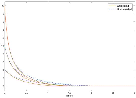
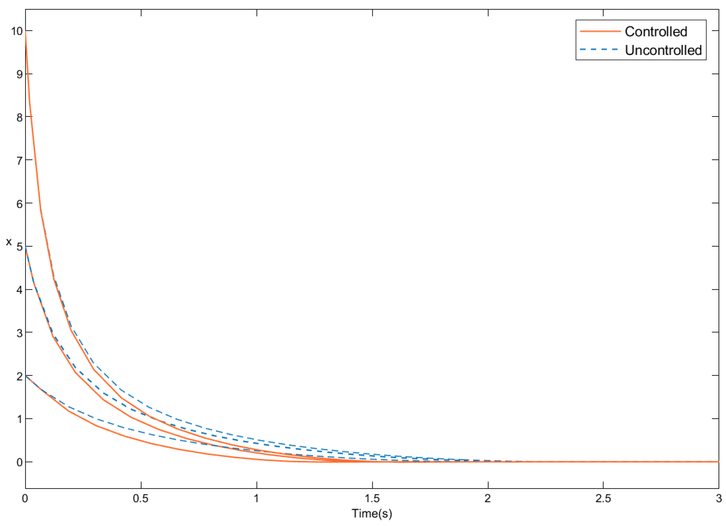
and hence, (91) and (92) is uniformly strongly passive. Now, it follows from i) of Corollary 4 that the negative feedback interconnection of (89) and (90), and (91) and (92) is fixed-time stable.

Figure 9 shows the controlled and the uncontrolled state x versus time for $x_0=2,5,10$, and $x_{\mathrm{c}0}=0$.

6. Conclusions

In this paper, we developed Lyapunov and converse Lyapunov theorems for fixed-time stability involving a new fixed-time scalar differential inequality. The regularity properties of the Lyapunov function satisfying this inequality were shown to strongly depend on the regularity properties of the settling time function. Furthermore, we merged the notions of fixed-time stability theory with dissipativity theory to develop the new notion of uniform strong dissipativity. In addition, we provided necessary and sufficient Kalman–Yakubovich–Popov conditions for characterizing uniform strong dissipativity via continuously differentiable storage functions and quadratic supply rates. Finally, using the concepts of uniform strong dissipativity for nonlinear dynamical systems with appropriate storage functions and supply rates, finite-time and fixed-time stability criteria for nonlinear feedback dynamical systems were given.

In future research, we will extend the notions of strong and uniform strong dissipativity to discrete-time systems and develop feedback interconnection stability results that guarantee finite-time and fixed-time stability. Furthermore, we will explore connections between uniform strong dissipativity theory and optimal and inverse optimal fixed-time stabilization using the Hamilton–Jacobi–Bellman theory, as well as provide connections to the classical time-optimal control problem. Since there can exist finite-time and fixed-time stable dynamical systems that do not admit a continuously differentiable value (i.e., Lyapunov) function that verifies the hypothesis of our fixed-time stability and uniform strong dissipativity theorems, a particularly important extension is the consideration of continuous Lyapunov functions leading to viscosity solutions of the resulting Hamilton–Jacobi–Bellman equation arising from the fixed-time optimal control problem.

References

- Roxin, E. On finite stability in control systems. Rend. Circ. Mat. Palermo 1966, 15, 273–282. [Google Scholar] [CrossRef]
- Bhat, S.P.; Bernstein, D.S. Finite-time stability of continuous autonomous systems. SIAM J. Control Optim. 2000, 38, 751–766. [Google Scholar] [CrossRef]
- Bhat, S.P.; Bernstein, D.S. Geometric homogeneity with applications to finite-time stability. Math. Control. Signals Syst. 2005, 17, 101–127. [Google Scholar] [CrossRef]
- Moulay, E.; Perruquetti, W. Finite time stability conditions for non-autonomous continuous systems. Int. J. Control 2008, 81, 797–803. [Google Scholar] [CrossRef]
- Haddad, W.M.; Nersesov, S.G.; Du, L. Finite-time stability for time-varying nonlinear dynamical systems. In Proceedings of the American Control Conference, Seattle, WA, USA, 11–13 June 2008; pp. 4135–4139. [Google Scholar]
- Andrieu, V.; Praly, L.; Astolfi, A. Homogeneous approximation, recursive observer design, and output feedback. SIAM J. Control Optim. 2008, 47, 1814–1850. [Google Scholar] [CrossRef]
- Polyakov, A. Nonlinear feedback design for fixed-time stabilization of linear control systems. IEEE Trans. Autom. Control 2012, 57, 2106–2110. [Google Scholar] [CrossRef]
- Polyakov, A.; Efimov, D.; Perruquetti, W. Finite-time and fixed-time stabilization: Implicit Lyapunov function approach. Automatica 2015, 51, 332–340. [Google Scholar] [CrossRef]
- Lu, W.; Liu, X.; Chen, T. A note on finite-time and fixed-time stability. Neural Netw. 2016, 81, 11–15. [Google Scholar] [CrossRef] [PubMed]
- Song, Y.; Wang, Y.; Holloway, J.; Krstic, M. Time-varying feedback for regulation of normal-form nonlinear systems in prescribed finite time. Automatica 2017, 83, 243–251. [Google Scholar] [CrossRef]
- Jiménez-Rodríguez, E.; Sánchez-Torres, J.D.; Loukianov, A.G. On optimal predefined-time stabilization. Int. J. Robust Nonlinear Control 2017, 27, 3620–3642. [Google Scholar] [CrossRef]
- Lopez-Ramirez, F.; Efimov, D.; Polyakov, A.; Perruquetti, W. Conditions for fixed-time stability and stabilization of continuous autonomous systems. Syst. Control. Lett. 2019, 129, 26–35. [Google Scholar] [CrossRef]
- Hu, C.; Yu, J.; Chen, Z.; Jiang, H.; Huang, T. Fixed-time stability of dynamical systems and fixed-time synchronization of coupled discontinuous neural networks. Neural Netw. 2017, 89, 74–83. [Google Scholar] [CrossRef] [PubMed]
- Willems, J.C. Dissipative dynamical systems, Part I: General theory. Arch. Rat. Mech. Anal. 1972, 45, 321–351. [Google Scholar] [CrossRef]
- Brogliato, B.; Lozano, R.; Maschke, B.; Egeland, O. Dissipative Systems Analysis and Control: Theory and Applications; Springer: London, UK, 2007. [Google Scholar] [CrossRef]
- Haddad, W.M.; Chellaboina, V. Nonlinear Dynamical Systems and Control: A Lyapunov-Based Approach; Princeton University Press: Princeton, NJ, USA, 2008. [Google Scholar]
- Haddad, W.M.; Somers, L.; Meskin, N. Finite time stability of nonlinear strongly dissipative feedback systems. Int. J. Control 2025, 98, 105–114. [Google Scholar] [CrossRef]
- Hill, D.J.; Moylan, P.J. Stability results for nonlinear feedback systems. Automatica 1977, 13, 377–382. [Google Scholar] [CrossRef]
- Hale, J.K. Ordinary Differential Equations, 2nd ed.; Wiley: New York, NY, USA, 1980. [Google Scholar]
- Agarwal, R.P.; Lakshmikantham, V. Uniqueness and Nonuniqueness Criteria for Ordinary Differential Equations; World Scientific: Singapore, 1993. [Google Scholar]
- Filippov, A.F. Differential Equations with Discontinuous Right-Hand Sides; Mathematics and Its Applications (Soviet Series); Kluwer Academic: Dordrecht, The Netherlands, 1988. [Google Scholar]
- Kawski, M. Stabilization of nonlinear systems in the plane. Syst. Control Lett. 1989, 12, 169–175. [Google Scholar] [CrossRef]
- Yoshizawa, T. Stability Theory by Liapunov’s Second Method; The Mathematical Society of Japan: Tokyo, Japan, 1966. [Google Scholar]
- Bhat, S.P.; Bernstein, D.S. Continuous, bounded, finite-time stabilization of the translational and rotational double integrators. In Proceedings of the IEEE International Conference on Control Applications, Dearborn, MI, USA, 15 September–18 November 1996; pp. 185–190. [Google Scholar] [CrossRef]
- Dahl, P. Solid friction damping of mechanical vibrations. AIAA J. 1976, 14, 1675–1682. [Google Scholar] [CrossRef]
- Åström, K.J. Control of systems with friction. In Proceedings of the Fourth International Conference on Motion and Vibration Control, Zurich, Switzerland, 25–28 August 1998; pp. 25–32. [Google Scholar]
- Mitrinovic, D.S.; Vasic, P.M. Analytic Inequalities; Springer: Berlin/Heidelberg, Germany, 1970. [Google Scholar]
Disclaimer/Publisher’s Note: The statements, opinions and data contained in all publications are solely those of the individual author(s) and contributor(s) and not of MDPI and/or the editor(s). MDPI and/or the editor(s) disclaim responsibility for any injury to people or property resulting from any ideas, methods, instructions or products referred to in the content. |
© 2025 by the authors. Licensee MDPI, Basel, Switzerland. This article is an open access article distributed under the terms and conditions of the Creative Commons Attribution (CC BY) license (https://creativecommons.org/licenses/by/4.0/).