A Robust Optimization Approach for E-Bus Charging and Discharging Scheduling with Vehicle-to-Grid Integration

Abstract

Electric buses (E-buses) are gaining popularity in urban transportation due to their environmental benefits and operational efficiency. However, large-scale integration of E-buses and Vehicle-to-Grid (V2G) technology introduces scheduling complexities for charging and discharging operations arising from uncertainties in energy consumption and load reduction requests. While prior studies have explored electric vehicle scheduling, few have considered robust optimization for E-bus fleets under uncertain parameters such as trip energy consumption and load reduction requests. This paper proposes a robust optimization approach for the charging and discharging scheduling problem at E-bus depots equipped with V2G. The problem is formulated as a robust mixed-integer linear program (MILP), incorporating real-world operational constraints including dual-port chargers, emergency charging, and demand response. A budgeted uncertainty set is used to model uncertainty in energy consumptions and discharging requests, providing a balance between robustness and conservatism. To ensure tractability, the robust counterpart is reformulated into a solvable MILP using duality theory. The effectiveness of the proposed model is validated through extensive computational experiments, including simulation-based performance assessments and out-of-sample tests. Experiment results demonstrate superior profitability and reliability compared to deterministic and box-uncertainty models, highlighting the practical effectiveness of the proposed approach.

1. Introduction

The growing awareness of the significant effects of climate change has prompted the strengthening of environmental policies and regulations aimed at reducing greenhouse gas emissions and carbon footprint. Concerns regarding air pollution and climate change have led to increased demand for cleaner transportation options. As a viable solution to this challenge, electric vehicles (EVs) are being rapidly adopted worldwide [1]. According to [2], EV sales keep rising and could reach around 17 million in 2024, which is more than one in five vehicles sold worldwide.

Moreover, this trend of electrification extends beyond personal vehicles to include commercial vehicles such as buses and trucks as well. Recently, transportation and logistics companies have started to convert their fleets to emission-free electric buses (E-buses) or electric trucks (E-trucks). Particularly, the introduction of E-buses has direct impacts on the public transportation system as well as urban environments. Since E-buses operate serve large numbers of passengers daily, their electrification can substantially reduce air pollution in densely populated areas. This shift not only helps improve public health by lowering exposure to harmful pollutants but also supports government efforts to meet emissions targets. Under the current policy, the number of E-buses is expected to increase sevenfold by 2035, and that of E-trucks could rise by about thirty times, supported by strict emission restrictions [2].

The introduction of E-buses has led transportation companies to renovate or reconstruct their depots to incorporate charging infrastructure. Consequently, traditional bus depots now serve a dual purpose, functioning not only as depots but also as charging stations for E-buses. For instance, Hamburger Hochbahn AG, the largest transportation company in Hamburg, Germany, recently converted its depot to accommodate a large fleet of E-buses [3]. Additionally, in 2022, Qatar launched the world’s largest E-bus depot [4]. Throughout this paper, the terms E-bus depot and charging station will be used interchangeably.

The rapid proliferation of EVs, including E-buses, and their integration into the power grid have introduced several challenges, such as insufficient charging infrastructure and increasing electricity demand for charging. As EV adoption continues to grow, effectively addressing these issues becomes increasingly critical. To tackle these challenges, alongside expanding the charging infrastructure, various smart charging technologies have been developed to efficiently utilize the limited charging resources. One of the key technologies is Vehicle-to-Grid (V2G) technology which enables bidirectional power transfer by allowing EVs not only to draw electricity from the grid during charging but also to supply stored energy back to the grid through discharging when needed [5,6].

When integrated with the grid through V2G, EVs can function as energy storage devices and play various roles within the power system [7]. For example, V2G technology can provide frequency regulation services, smooth power load variation, reduce operational costs, and lower the greenhouse gas emissions [8,9]. Particularly, by optimizing the charging and discharging schedules, companies can generate additional revenue through energy trading. Although each EV has a relatively small battery capacity, when aggregated, particularly in the case of a fleet of E-buses, it provides a substantial capacity that can create opportunities for companies to generate additional revenue. Therefore, it is crucial to strategically determine the timing and amount of charging and discharging of E-buses to maximize profits while ensuring that all scheduled trips are conducted as planned.

From a charging and discharging scheduling perspective, a key difference between E-buses and personal EVs lies not only in their large battery capacity but also in whether charging station operators have access to the vehicle information in advance. For typical charging stations serving personal EVs, the arrival and departure times, as well as the battery charging levels upon arrival, are typically unknown beforehand. In contrast, since both E-bus fleets and depots are managed and operated by the same transportation company, the companies can have prior knowledge of vehicle schedules and State-of-Charge (SoC) levels. This allows E-bus charging operations to be planned more efficiently with less uncertainty compared to standard charging stations for personal EVs.

By integrating with the grid through V2G, E-buses can generate additional revenue by supplying electricity to the grid. This is particularly beneficial when participating in Demand Response (DR) programs, where E-buses can play a crucial role in stabilizing the grid during peak hours [10,11]. In a typical DR scenario, grid operators request load reductions during peak hours to maintain a stable electricity supply. In response, charging station operators discharge power back into the grid, generating additional revenue through DR contracts. These contracts require operators to supply the requested amount of energy to fulfill their obligations. Failure to meet this requirement may result in a reduced compensation.

To maximize the benefits of V2G and DR programs, establishing an optimal charging and discharging schedule at charging stations is essential. An effective schedule allows operators to reduce operational costs by strategically timing charging during off-peak hours and discharging power during peak hours, while complying with the predetermined trip schedules of E-buses. Moreover, an optimized schedule ensures that the discharge amounts required by DR contracts are met, thereby avoiding penalties or reductions in compensation.

A significant challenge in establishing an efficient charging and discharging schedule for E-buses arises from various uncertainties. One major source of uncertainty is unpredictable discharging requests from the grid, driven by the inherently variable nature of electricity demand and fluctuations in renewable energy generation. As a result, charging station operators often lack prior knowledge of the exact reduction amounts needed when planning their schedules. Another critical source of uncertainty lies in the energy consumption of E-bus during daily operations, which is affected by various factors such as weather, temperature, traffic conditions, and crowding levels [12,13]. This uncertainty can lead to significant deviations between anticipated and actual energy usage, potentially resulting in insufficient SoC during trips. Failure to adequately account for these uncertainties can lead to increased costs and hinder the fulfillment of DR commitments, reducing overall profitability.

Robust optimization (RO) is a widely used framework for decision-making under uncertainty, particularly when the exact probability distributions of uncertain parameters are not available. Unlike stochastic programming, which aims to optimize expected performance based on known distributions, RO seeks solutions that are feasible and effective across all possible realizations within a predefined uncertainty set. This perspective is especially suitable for operational problems such as E-bus scheduling, where uncertainties in energy consumption and discharging demand are affected by various external factors that are difficult to model probabilistically. This makes RO particularly well-suited for the E-bus charging and discharging scheduling problem, where the underlying uncertainties cannot be accurately characterized using probability distributions. Moreover, given the operational importance of ensuring feasibility under all conditions (e.g., avoiding undercharging of buses or failing to meet grid requests), an RO-based approach is essential. RO provides a mathematically rigorous way to capture such requirements by guaranteeing performance across all realizations within a defined uncertainty set.

In this paper, we propose a RO approach to address the charging and discharging scheduling problem at E-bus charging stations equipped with V2G technology. The model considers key operational constraints such as charger port assignments, emergency charging, and demand response participation, while accounting for uncertainties in energy consumption and discharging requests from the grid. We formulate this problem as a robust mixed-integer linear program (MILP), where uncertainty is represented via budgeted uncertainty sets that allow for a tunable trade-off between robustness and conservatism of solutions. In particular, budgets were established to reflect the cumulative nature of uncertainties over time. To ensure tractability, the robust counterpart is reformulated using linear programming duality, resulting in a solvable MILP model. This mathematical programming framework enables the derivation of robust and cost-effective schedules that minimize the risk of battery depletion and performance degradation under worst-case scenarios. The effectiveness of the proposed approach is demonstrated through extensive computational experiments, including simulation-based performance assessments and out-of-sample tests. The test results clearly indicate the superior profitability and reliability compared to deterministic and box-uncertainty models, highlighting the practical effectiveness of the proposed approach. The key methodological contributions of this work lie in the construction of a robust scheduling model for the E-bus depot, and the development of a tractable reformulation that preserves robustness while enabling efficient optimization. These contributions place the work within the domain of mathematical programming.

The remainder of this paper is organized as follows. Section 2 reviews the related literature. In Section 3, we present a MILP model for the deterministic version of the problem. In Section 4, we develop a RO model that accounts for uncertainties in energy consumption and reduction requests. Section 5 presents the results of computational experiments to validate the effectiveness of the proposed model. Finally, Section 6 provides concluding remarks and explores potential future research directions.

2. Literature Review

Early studies on EV charging scheduling mainly focused on optimizing charging operations under various objective functions without considering discharging or V2G integration. For example, linear programming (LP)-based methods have been proposed to optimize both the load aggregator’s revenue and customer costs in static and dynamic settings [14]. Similarly, a metaheuristic approach that combines a memetic algorithm with a variable neighborhood search was applied to minimize total tardiness for EVs, also considering both static and dynamic settings [15]. Charging cost minimization was addressed in [16] using a bi-level optimization approach that assigns EVs to chargers at the upper level and determines the detailed charging schedule for each EV at the lower level. While these studies provide effective strategies for EV charging scheduling under various objectives, they do not consider discharging operations under V2G technology.

The introduction of V2G technology has added new dimensions to the EV charging scheduling problem, as both charging and discharging operations must now be coordinated. As a result, research has increasingly focused on addressing these V2G-specific challenges. For example, in [17], a charging and discharging scheduling problem for EVs in parking lots was addressed. To maximize profits of EV owners, a mathematical model incorporating practical constraints such as charging/discharging limits and minimum/maximum SoC levels was developed. Another approach introduced a bi-objective optimization model balancing time-aware fairness and cost efficiency [18]. More recently, an iterative multi-stage optimization method was proposed to enhance V2G operations, including charging/discharging scheduling [19]. These studies highlight the growing interest in optimizing both charging and discharging operations for EVs. However, research specifically targeting E-bus depots, especially under V2G integration, remains limited.

In addition to individual EVs, there is also growing interest in addressing the charging scheduling problem for E-bus depots [20,21,22,23,24,25]. For example, in [23], an E-bus charging scheduling problem was addressed by optimizing charging locations and time slots to minimize total charging costs. The study employed Lagrangian relaxation to decompose the fleet into individual buses and used a dynamic programming algorithm for the single-bus problem.

However, as highlighted in the recent review paper [26], research on the charging and discharging scheduling problem for E-buses with V2G technology remains limited, despite its growing importance. In [27], a comparison between V2G-capable electric school buses and traditional diesel bus fleets demonstrated clear advantages in terms of cost and profit. An MILP model aimed at maximizing depot operator profits was introduced in [28], assuming a deterministic framework where all parameters were known in advance. Unlike this approach, a stochastic programming model that incorporates uncertainties in real-time market parameters and considers multiple objectives was developed in [29].

While stochastic programming approaches have been applied to E-bus scheduling with V2G, they require information on probability distributions, which may not always be available. In contrast, RO relies solely on a well-defined uncertainty set, making it particularly effective when information about uncertainty is limited. RO is a widely adopted approach for handling data uncertainty, aiming to minimize worst-case costs while ensuring feasible solutions for all possible realizations of uncertainty [30].

Although RO approaches have not been directly applied to the E-bus scheduling problem with V2G, several studies have explored similar problem settings. For example, a multi-objective RO approach for charging and discharging scheduling problem of individual EVs was proposed in [31] considering uncertain photovoltaic energy generation. An E-bus scheduling problem that integrates trip assignment and charging scheduling under uncertain travel times was addressed in [32]. A RO method for EV charging scheduling with energy consumption uncertainty, excluding V2G operations, was introduced in [33]. Additionally, an adjustable RO approach considering uncertainties in renewable energy sources and SoC levels was proposed in [34]. In [35], a RO approach was developed for V2G scheduling accounting for range anxiety. These studies highlight the need for a RO approach tailored specifically to the E-bus charging and discharging scheduling problem with V2G technology, which remains an underexplored yet critical area for enhancing grid stability and profitability.

Table 1. Summary of the literature on EV and E-bus charging scheduling problems.

Ref.	EV Fleet Type	V2G Integration	Uncertainty	Objective	Methods
[14]	Private EVs	-	-	Aggregator revenue, Customer cost	Linear programming
[15]	Private EVs	-	-	Total tardiness	Metaheuristics
[16]	Private EVs	-	-	Charging cost	Bi-level programming
[17]	Private EVs in parking lots	✓	-	EV owner profit	Nonlinear programming
[18]	Private EVs	✓	–	Time-aware fairness, Cost efficiency	Bi-objective optimization
[19]	Private EVs	✓	–	Total costs	Multi-stage optimization
[20]	E-buses	–	–	Charging costs	Linear programming
[21]	E-buses	–	–	Operating costs	Second-order conic programming
[22]	E-buses	–	–	Charging costs	Real-time optimization
[23]	E-buses	–	–	Total costs	Lagrangian relaxation
[24]	E-buses	–	–	Charging time	Lagrangian relaxation
[25]	E-buses	–	–	Total costs	Branch-and-price, Adaptive large neighborhood search
[27]	E-school buses	✓	–	–	Comparative analysis
[28]	E-buses	✓	–	Daily profit	Mixed integer linear programming
[29]	E-buses	✓	Day-ahead forecast	Total costs	Mixed integer linear programming, Stochastic model
[31]	Private EVs	✓	PV Generation	Charging costs, Load fluctuation, PV consumption	Robust optimization
[32]	E-buses	–	Travel time	Operational cost	Robust optimization, Branch-and-price
[33]	E-buses	–	Energy consumption	Total costs	Robust optimization
[34]	Private EVs	✓	Wind power, EV SoCs	Total costs	Adjustable robust optimization
[35]	Private EVs	✓	Range anxiety	Total costs	Robust optimization, Benders decomposition
This study	E-buses	✓	Energy consumption, DR Requests	Total profits	Robust optimization

provides a summary of the literature on charging scheduling problems with EVs and E-buses.

3. Deterministic Optimization Model

3.1. Problem Description

In this section, we present a deterministic MILP model for the charging and discharging scheduling problem for E-bus depots equipped with V2G technology, aiming to determine the optimal charging and discharging amounts for each E-bus over a planning horizon. For the depot operator, charging E-buses incurs costs, while discharging electricity back to the grid generates revenue. The objective is to maximize profit by efficiently coordinating charging and discharging schedules, considering predetermined E-bus trip schedules, dynamic electricity prices, and various operational constraints.

A set of E-buses is defined as $\mathcal{B}=\{1,\dots ,NB\}$. The planning horizon is discretized into a set of time periods $\mathcal{T}=\{1,\dots ,NT\}$. Each bus $i\in \mathcal{B}$ has a set of trips ${\mathcal{J}}_i$ to cover within the planning horizon, where the total number of trips for bus i is denoted by $N{J}_i$.

For each trip $j\in {\mathcal{J}}_i$, the energy consumption is denoted by $c_{ij}$ and is assumed to be uncertain. In addition, let $s_{ij}$ denote the period when bus i departs from the depot for trip j, and $t_{ij}$ denote the period when the bus returns to the depot after completing the trip. The interval $[s_{ij},s_{ij}+1,\dots ,t_{ij}]$ is denoted by ${\mathcal{S}}_{ij}$, which represents the set of time periods during which bus i is on the j-th trip and thus unavailable for charging or discharging. We assume that for each bus i, the trips in $N{J}_i$ are indexed in ascending order and do not overlap. That is, $1\le s_{i1}<t_{i1}<s_{i2}<t_{i2}<\cdots <s_{i{J}_i}<t_{i{J}_i}\le NT$. The set of time periods during which bus i is on a trip and not available at the depot is denoted by ${\mathcal{S}}_i$, that is, ${\mathcal{S}}_i={\cup }_{j\in {\mathcal{J}}_i}{\mathcal{S}}_{ij}$. The set of time periods during which bus i is at the depot is denoted by ${\mathcal{T}}_i$, given by ${\mathcal{T}}_i=\mathcal{T}\setminus {\mathcal{S}}_i$.

The set of time periods corresponding to peak hours is denoted by $\mathcal{H}\subseteq \mathcal{T}$. We assume that the grid operator makes load reductions requests multiple times during peak hours on an hourly basis. The set of all requests is denoted by $\mathcal{K}=\{1,\dots ,NK\}$. The time periods corresponding to the k-th request are denoted by a subset ${\mathcal{H}}_k\subseteq \mathcal{H}$, as illustrated in Figure 1. Each request $k\in \mathcal{K}$ specifies a required reduction amount $r_k$, which is uncertain. The cumulative amount of these reductions must be satisfied over the course of the peak hours. Specifically, for each $k\in \mathcal{K}$, the total amount across up to the k-th request, ${\sum }_{j=1}^k{r}_j$, must be met by the corresponding reduction during the time periods in ${\bigcup }_{j=1}^k{\mathcal{H}}_j$.

The number of available chargers in period t is denoted as $N_t$. Specifically, we consider a dual-port charging system [36], as illustrated in Figure 2, where each charger is equipped with two ports. The charging and discharging rate, as well as the maximum capacity, depend on the number of ports connected. For example, both ports can be connected to a single bus for fast charging, or one port can be connected to each of two buses for simultaneous charging. The maximum charging and discharging rate per unit time is assumed to be proportional to the number of connected ports. The set $\mathcal{P}=\{1,\dots ,NP\}$ represents the number of ports available for charging. As we consider dual-port chargers, $NP=2$. This set can be interpreted as the set of charging modes, where $p=1$ corresponds to a regular charging mode using a single port, and $p=2$ corresponds to a fast charging mode with both ports.

The efficiencies of charging and discharging for bus i is denoted as ${\eta }_i^{ch}$ and ${\eta }_i^{dis}$, respectively. The capacity of bus i’s battery is denoted as $B_i$. $K_p^{ch}$ and $K_p^{dis}$ represent the maximum charging and discharging amounts when using port p. Unit prices of charging and discharging in period t is denoted as $P_t^{ch}$ and $P_t^{dis}$, respectively. We assume that, if a bus is unable to charge the required amount of energy necessary for its trip, it can obtain emergency charging from external sources. The cost of emergency charging, denoted as $P_t^{exp}$, is assumed to be higher than $P_t^{ch}$. The nomenclature is summarized in

Table 2. Nomenclature.

Sets
$\mathcal{B}$	set of buses ($\mathcal{B}=\{1,\dots ,NB\}$)
$\mathcal{T}$	set of time periods ($\mathcal{T}=\{1,\dots ,NT\}$)
${\mathcal{J}}_i$	set of trips for bus i ($j\in {\mathcal{J}}_i=\{1,\dots ,N{J}_i\}$)
${\mathcal{T}}_i$	set of time periods during which bus i is at the charging station
${\mathcal{S}}_i$	set of time periods during which bus i is in operation
$\mathcal{H}$	set of time periods corresponding to peak hours ($\mathcal{H}=\{1,\dots ,NH\})$
${\mathcal{H}}_k$	set of time periods corresponding to k-th loadreduction requests
$\mathcal{K}$	set of load reduction requests ($\mathcal{K}=\{1,\dots ,NK\})$
$\mathcal{P}$	set of ports ($\mathcal{P}=\{1,\dots ,NP\}$)
Parameters
$c_{ij}$	energy consumption of j-th trip of bus i
$s_{ij}$/$t_{ij}$	start time/finish time of j-th trip of bus i
${\mathcal{S}}_{ij}$	$:=[s_{ij},s_{ij}+1,\dots ,t_{ij}]$
$r_k$	required load reduction amount of k-th request
$N_t$	number of available chargers in period t
${\eta }_i^{ch}/{\eta }_i^{dis}$	charging and discharging efficiencies for bus i
$B_i$	battery capacity of bus i
$K_p^{ch}$/$K_p^{dis}$	maximum charging/discharging amount using port p
$P_t^{ch}/P_t^{dis}$	charging and discharging prices in period t
$P_t^{exp}$	expensive emergency charging price in period t
Variables
$x_{it}$	charging amount of bus i at period t
$y_{it}$	discharging amount of bus i at period t
$x{r}_{itp}$	$=1$ if bus i is charged in period t with port p
$y{r}_{itp}$	$=1$ if bus i is discharged in period t with port p
$z_{it}$	emergency charging amount of bus i at period t
$u_{it}$	SoC level of bus i at the end of period t

.

3.2. Deterministic Optimization Model

We first present a deterministic MILP model for the problem, which assumes that both the energy consumption $c_{ij}$ and the amounts of load reduction requests $r_k$ are known with certainty. For the model, we define the decision variables as follows. Let $x_{it}$ and $y_{it}$ represent the charging and discharging amounts of bus i in period t, respectively. The binary variables $x{r}_{itp}$ and $y{r}_{itp}$ indicate whether bus i is being charged or discharged in period t using port p, respectively. The variable $z_{it}$ represents the amount of emergency charging for bus i in period t. Finally, the variable $u_{it}$ represents the SoC level of bus i at the end of period t. The deterministic MILP model is formulated as follows:

$$\begin{array}{cc}\hfill \mathrm{maximize}& \sum _{i\in \mathcal{B}}\sum _{t\in {\mathcal{T}}_i}\left(P_t^{dis}{y}_{it}-P_t^{ch}{x}_{it}-P_t^{exp}{z}_{it}\right)\hfill \end{array}$$

(1)

$$\begin{array}{ccc}\hfill \mathrm{subject}\mathrm{to}& u_{it}=u_{i,t-1}+{\eta }_i^{ch}(x_{it}+z_{it})-{\eta }_i^{dis}{y}_{it},\hfill & \hfill \forall i\in \mathcal{B},t\in {\mathcal{T}}_i,\end{array}$$

(2)

$$\begin{array}{ccc}\hfill & u_{i,t_{ij}}=u_{i,s_{ij}-1}-c_{ij},\hfill & \hfill \forall i\in \mathcal{B},j\in {\mathcal{J}}_i,\end{array}$$

(3)

$$\begin{array}{ccc}\hfill & 0\le u_{it}\le B_i,\hfill & \hfill \forall i\in \mathcal{B},t\in {\mathcal{T}}_i,\end{array}$$

(4)

$$\begin{array}{ccc}\hfill & \sum _{l=1}^k\sum _{t\in {\mathcal{H}}_l}\sum _{i\in \mathcal{B}}({\eta }_i^{dis}{y}_{it}-{\eta }_i^{ch}{x}_{it})\ge \sum _{l=1}^k{r}_l,\hfill & \hfill \forall k\in \mathcal{K},\end{array}$$

(5)

$$\begin{array}{ccc}\hfill & x_{it}\le \sum _{p\in \mathcal{P}}{K}_p^{ch}x{r}_{itp},\hfill & \hfill \forall i\in \mathcal{B},t\in {\mathcal{T}}_i,\end{array}$$

(6)

$$\begin{array}{ccc}\hfill & y_{it}\le \sum _{p\in \mathcal{P}}{K}_p^{dis}y{r}_{itp},\hfill & \hfill \forall i\in \mathcal{B},t\in {\mathcal{T}}_i,\end{array}$$

(7)

$$\begin{array}{ccc}\hfill & \sum _{p\in \mathcal{P}}\left(x{r}_{itp}+y{r}_{itp}\right)\le 1,\hfill & \hfill \forall i\in \mathcal{B},t\in {\mathcal{T}}_i,\end{array}$$

(8)

$$\begin{array}{ccc}\hfill & \sum _{i\in \mathcal{B}}\sum _{p\in \mathcal{P}}p\left(x{r}_{itp}+y{r}_{itp}\right)\le N_t·NP,\hfill & \hfill \forall t\in \mathcal{T},\end{array}$$

(9)

$$\begin{array}{ccc}\hfill & x_{it},y_{it},z_{it}\ge 0,\hfill & \hfill \forall i\in \mathcal{B},t\in {\mathcal{T}}_i,\end{array}$$

(10)

$$\begin{array}{ccc}\hfill & x{r}_{itp},y{r}_{itp}\in \{0,1\},\hfill & \hfill \forall i\in \mathcal{B},t\in {\mathcal{T}}_i,p\in \mathcal{P}.\end{array}$$

(11)

The objective function (1) maximizes the net profit for the depot operator, which is calculated as the discharging revenue minus the costs of regular and emergency charging. Constraints (2) and (3) represent the balance equations for the battery SoC levels. Constraints (2) apply when the bus is stationed at the depot, ensuring that the SoC level at the end of period t is equal to the SoC level at the end of period $t-1$ plus the net charging amount, while considering the charging and discharging efficiencies ${\eta }_i^{ch}$ and ${\eta }_i^{dis}$. Constraints (3) account for changes in the SoC level due to the j-th trip of bus i. It ensures that the SoC level at the end of the trip, $t_{ij}$, is equal to the SoC level at the start of the trip, $s_{ij}-1$, minus the energy consumption $c_{ij}$ required for the trip. Constraints (4) ensure that the SoC level remains within the battery capacity and is nonnegative.

Constraints (5) represent the net discharge requirement under DR, ensuring that the cumulative net discharge up to the k-th request is greater than or equal to the cumulative requested amount up to that point. Constraints (6) and (7) restrict the maximum charging and discharging amounts with respect to the number of used ports, respectively. Constraints (8) enforce mutual exclusivity between charging and discharging operations in a given time period and ensures that only one type of port is used at a time for a bus. Constraints (9) enforce the port availability limit, ensuring that the total number of ports used across all buses does not exceed the installed ports. Constraints (10) and (11) define the domain of variables, ensuring nonnegativity and binary conditions, respectively.

4. Robust Optimization Model

4.1. Uncertainty Sets

In the RO model, we consider two types of uncertain parameters: the energy consumption amount $c_{ij}$ for j-th trip of bus i and the amounts of load reduction requests $r_k$. Specifically, we model $c_{ij}$ as a bounded uncertain parameter which takes values within the interval $[{\overline{c}}_{ij}-{\widehat{c}}_{ij},{\overline{c}}_{ij}+{\widehat{c}}_{ij}]$ where ${\overline{c}}_{ij}$ and ${\widehat{c}}_{ij}$ represent the nominal value and maximum deviation of $c_{ij}$, respectively. The scaled deviation of $c_{ij}$ is defined as $w_{ij}:=(c_{ij}-{\overline{c}}_{ij})/{\widehat{c}}_{ij}$ which takes values within the interval $[-1,1]$. In addition, we define a vector of the scaled deviation for bus i as ${\mathbf{w}}_i:=(w_{i1},w_{i2},\dots ,w_{i,N{J}_i})$. Then, a set $\left\{{\mathbf{w}}_i|-1\le w_{ij}\le 1,\forall j\in {\mathcal{J}}_i\right\}$ incorporates all possible realizations of uncertain parameters ${\mathbf{w}}_i$. From the structure of the set, it is denoted as a box uncertainty set [37].

However, since it is implausible that all components of ${\mathbf{w}}_i$ take their worst-case values simultaneously, finding a robust solution that remains feasible for all possible realization of ${\mathbf{w}}_i$ under the box uncertainty set can lead to overly conservative results. In this regard, we assume that there are limited budgets of uncertainty [38] which is widely used to avoid over-conservatism of the RO approaches. Particularly, the budget parameter ${\Gamma }_{ij}^c$ is imposed to restrict the amount of cumulative deviations for the first j trips of bus i, that is, ${\sum }_{l=0}^j\left|w_{il}\right|\le {\Gamma }_{ij}^c$ for all $j\in {\mathcal{J}}_i$. Following [39], we assume that ${\Gamma }_{ij}^c\in [0,j]$ and ${\Gamma }_{i1}^c\le {\Gamma }_{i2}^c\le \cdots \le {\Gamma }_{i,N{J}_i}^c$. Then, the budgeted uncertainty set ${\mathcal{W}}_i$ can be defined as follows:

$${\mathcal{W}}_i=\left\{{\mathbf{w}}_i|-1\le w_{ij}\le 1,\sum _{l=1}^j\left|w_{il}\right|\le {\Gamma }_{ij}^c,\forall j\in {\mathcal{J}}_i\right\}.$$

The budgeted uncertainty set ${\mathcal{W}}_i$ controls the degree of conservatism in the RO model by limiting how many parameters can simultaneously deviate from their nominal values. This is governed by a budget parameter ${\Gamma }_{ij}^c$, which allows the model to adjust the level of protection against uncertainty. A smaller budget results in a less conservative solution, potentially increasing profit but risking infeasibility under uncertainty. In contrast, a larger budget yields a more robust but overly conservative solution. For instance, setting ${\Gamma }_{ij}^c=0$ implies $w_{i1}=\cdots =w_{ij}=0$, meaning that no uncertainty is considered in ${\mathbf{w}}_i$, representing the deterministic case. Conversely, when ${\Gamma }_{ij}^c=j$, the components $w_{i1},\dots ,w_{ij}$ can simultaneously deviate to their worst-case values. In this case, the budget uncertainty set becomes equivalent to the box uncertainty set where the full range of uncertainty is incorporated [37].

Similarly, the uncertain amounts of load reduction requests, $r_k$, are assumed to take values within the interval $[{\overline{r}}_k-{\widehat{r}}_k,{\overline{r}}_k+{\widehat{r}}_k]$ where ${\overline{r}}_k$ and ${\widehat{r}}_k$ represent the nominal value and deviation of $r_k$, respectively. The scaled deviation of $r_k$ is defined as $v_k:=(r_k-{\overline{r}}_k)/{\widehat{r}}_k$ which takes values within the interval $[-1,1]$. We define a vector $\mathbf{v}:=(v_1,v_2,\dots ,v_{NK}$) and the corresponding uncertainty set $\mathcal{V}$ as follows:

$$\mathcal{V}=\left\{\mathbf{v}|-1\le v_k\le 1,\sum _{l=1}^k\left|v_l\right|\le {\Gamma }_k^d,\forall k\in \mathcal{K}\right\}.$$

The size of uncertainty set $\mathcal{V}$ is controlled by the budget parameter ${\Gamma }_k^d$, which adjusts the level of conservatism. Similar to ${\Gamma }_{ij}^c$ in the previous case, when ${\Gamma }_k^d=0$, uncertainty is not considered, while ${\Gamma }_k^d=k$ fully accounts for it. We assume ${\Gamma }_k^d$ takes values within $[0,k]$ for all $k\in \mathcal{K}$. The impact of budget parameters ${\Gamma }_{ij}^c$ and ${\Gamma }_k^d$ is examined in Section 5.4.

4.2. Robust Optimization Model

Now, we formulate the RO model. In the RO model, the SoC level balance constraints (3) cannot be satisfied for all possible realizations of $c_{ij}$ since they are formulated as equality constraints. Furthermore, because these constraints are linked to constraints (2) through the SoC variables $u_{it}$, constraints (2) also cannot be satisfied for all possible realizations. Therefore, these constraints must be reformulated as inequalities.

To facilitate the reformulation, we introduce additional notation for clarity. Let ${\mathcal{T}}_i\left(t\right)$ denote the set of time periods before period t during which bus i is in the charging station, i.e., ${\mathcal{T}}_i\left(t\right):=\{\tau \in {\mathcal{T}}_i:\tau \le t\}$. Similarly, let ${\mathcal{J}}_i\left(t\right)$ be the subset of ${\mathcal{J}}_i$ containing trips that are completed before period t, i.e., $t_{ij}<t$ for $j\in {\mathcal{J}}_i\left(t\right)$. The index of the last trip in ${\mathcal{J}}_i\left(t\right)$ is denoted by $j_{it}$. In other words, $j_{it}$ represents the last trip of bus i which is completed before period t.

From constraints (2) and (3), the variable $u_{it}$ can be expressed in an aggregated form as

$$u_{it}=u_{i0}+\sum _{\tau \in {\mathcal{T}}_i\left(t\right)}\left({\eta }_i^{ch}(x_{i\tau }+z_{i\tau })-{\eta }_i^{dis}{y}_{i\tau }\right)-\sum _{j\in {\mathcal{J}}_i\left(t\right)}({\overline{c}}_{ij}+{\widehat{c}}_{ij}{w}_{ij}),$$

which represents the SoC level of bus i at period t as the initial SoC level $u_{i0}$, plus the cumulative net charging amount up to period t, while accounting for the total energy consumption from trips completed before t.

Using the above equation, the variables $u_{it}$ can be eliminated from the formulation. Consequently, the following constraints (12) and (13) for the RO model are derived from the nonnegativity and battery capacity constraints (4), respectively:

$$u_{i0}+{\sum }_{\tau \in {\mathcal{T}}_i\left(t\right)}\left({\eta }_i^{ch}(x_{i\tau }+z_{i\tau })-{\eta }_i^{dis}{y}_{i\tau }\right)-{\sum }_{j\in {\mathcal{J}}_i\left(t\right)}({\overline{c}}_{ij}+{\widehat{c}}_{ij}{w}_{ij})\ge 0,\forall i\in \mathcal{B},t\in {\mathcal{T}}_i,{\mathbf{w}}_i\in {\mathcal{W}}_i,$$

(12)

$$u_{i0}+{\sum }_{k\in {\mathcal{T}}_i\left(t\right)}\left({\eta }_i^{ch}(x_{ik}+z_{ik})-{\eta }_i^{dis}{y}_{ik}\right)-{\sum }_{j\in {\mathcal{J}}_i\left(t\right)}({\overline{c}}_{ij}+{\widehat{c}}_{ij}{w}_{ij})\le B_i,\forall i\in \mathcal{B},t\in {\mathcal{T}}_i,{\mathbf{w}}_i\in {\mathcal{W}}_i.$$

(13)

Similarly, the net discharge requirement constraints (5) can be modified for the RO model as follows:

$$\sum _{l=1}^k\sum _{t\in {\mathcal{H}}_l}\sum _{i\in \mathcal{B}}({\eta }_i^{dis}{y}_{it}-{\eta }_i^{ch}{x}_{it})\ge \sum _{l=1}^k({\overline{r}}_l+{\widehat{r}}_l{v}_l),\forall k\in \mathcal{K},\mathbf{v}\in \mathcal{V}.$$

(14)

Incorporating the above constraints, the RO model is formulated as follows:

$$\begin{array}{c}\hfill \left(RO\right):=\left\{max\left(1\right):\mathrm{s}.\mathrm{t}.\left(6\right)-\left(11\right),\left(12\right),\left(13\right),\left(14\right)\right\}.\end{array}$$

4.3. Tractable Reformulation of Robust Counterparts

Since the numbers of possible realizations of ${\mathbf{w}}_i$ and $\mathbf{v}$ are infinite, there are infinite number of constraints (12)–(14), making the $\left(RO\right)$ model intractable. To address this, we derive a computationally tractable reformulation of $\left(RO\right)$. It is well-known that when polyhedral uncertainty sets are considered, the $\left(RO\right)$ model can be reformulated as a tractable MILP model [38]. In this process, we follow a similar approach to [39] in deriving the tractable reformulation of the robust counterpart.

Because constraint (12) is a “greater than or equal to” type of constraint with uncertainty on the left-hand side, the feasibility for all ${\mathbf{w}}_i$ can be verified by minimizing the left-hand side of the constraint over the uncertainty set. This is equivalent to maximizing the term ${\sum }_{j\in {\mathcal{J}}_i\left(t\right)}{\widehat{c}}_{ij}{w}_{ij}$ over the uncertainty set ${\mathcal{W}}_i$. Conversely, constraint (13) has the opposite direction, meaning that ${\sum }_{j\in {\mathcal{J}}_i\left(t\right)}{\widehat{c}}_{ij}{w}_{ij}$ is minimized over ${\mathcal{W}}_i$.

Due to the symmetry of ${\mathcal{W}}_i$, both optimization problems over ${\mathcal{W}}_i$ can be reduced to a single optimization problem. Since the deviation ${\widehat{c}}_{ij}$ is nonnegative, the worst-case scenario occurs when $w_{ij}\ge 0$. Consequently, the constraints $-1\le w_{ij}\le 1$ and ${\sum }_{l=1}^j\left|w_{il}\right|$ can be replaced with $0\le w_{ij}\le 1$ and ${\sum }_{l=1}^j{w}_{il}$, respectively, leading to the following maximization problem $P(i,t)$ for $i\in \mathcal{B}$, $t\in {\mathcal{T}}_i$:

$$\begin{array}{cc}\hfill P(i,t)=max& \sum _{k\in {\mathcal{J}}_i\left(t\right)}{\widehat{c}}_{ik}{w}_{ik}\hfill \end{array}$$

(15)

$$\begin{array}{cc}\hfill \mathrm{s}.\mathrm{t}.& \sum _{k\in {\mathcal{J}}_i\left(t\right)}{w}_{ik}\le {\Gamma }_{i,j_{it}}^c,\hfill \end{array}$$

(16)

$$\begin{array}{cccc}\hfill & 0\le w_{ik}\le 1,\hfill & \hfill & \forall k\in {\mathcal{J}}_i\left(t\right).\hfill \end{array}$$

(17)

Note that the term ${\Gamma }_{i,j_{it}}^c$ in constraint (16) represents the budget parameter applied to the trips of bus i that are completed before period t.

Using the duality theorem of linear programming, the dual problem $D(i,t)$ of $P(i,t)$ can be derived. Let ${\lambda }_{it}$ and ${\mu }_{itk}$ be the dual variables associated with constraints (16) and (17), respectively. Then, the dual problem $D(i,t)$ is formulated as follows:

$$\begin{array}{cc}\hfill D(i,t)=min& {\lambda }_{it}{\Gamma }_{i,j_{it}}^c+\sum _{k\in {\mathcal{J}}_i\left(t\right)}{\mu }_{itk}\hfill \end{array}$$

(18)

$$\begin{array}{cccc}\hfill \mathrm{s}.\mathrm{t}.& {\lambda }_{it}+{\mu }_{itk}\ge {\widehat{c}}_{ik},\hfill & \hfill & \forall k\in {\mathcal{J}}_i\left(t\right),\hfill \end{array}$$

(19)

$$\begin{array}{cc}\hfill & {\lambda }_{it}\ge 0,\hfill \end{array}$$

(20)

$$\begin{array}{cccc}\hfill & {\mu }_{itk}\ge 0,\hfill & \hfill & \forall k\in {\mathcal{J}}_i\left(t\right).\hfill \end{array}$$

(21)

Since it is a feasible and bounded linear program, the optimal objective value of $D(i,t)$ is equal to that of $P(i,t)$ due to strong duality. Therefore, the uncertain terms in constraints (12) and (13) can be replaced by $D(i,t)$.

Similarly, the net discharging requirement constraint (14) can be reformulated. The primal problem $P\left(k\right)$, which determines the maximum deviation of the uncertainty in constraint (14) given the set $\mathcal{V}$, is formulated as follows:

$$\begin{array}{cc}\hfill P\left(k\right)=max& \sum _{l=1}^k{\widehat{r}}_l{v}_l\hfill \end{array}$$

(22)

$$\begin{array}{cc}\hfill \mathrm{s}.\mathrm{t}.& \sum _{l=1}^k{v}_l\le {\Gamma }_k^d,\hfill \end{array}$$

(23)

$$\begin{array}{ccc}\hfill & 0\le v_l\le 1,\hfill & \hfill \forall l=1,\cdots ,k.\end{array}$$

(24)

Let ${\xi }_k$ and ${\varphi }_{kl}$ be the dual variables associated with constraints (23) and (24), respectively. Then, the corresponding dual problem $D\left(k\right)$ is formulated as follows:

$$\begin{array}{cc}\hfill D\left(k\right)=min& {\xi }_k{\Gamma }_k^d+\sum _{l=1}^k{\varphi }_{kl}\hfill \end{array}$$

(25)

$$\begin{array}{ccc}\hfill \mathrm{s}.\mathrm{t}.& {\xi }_k+{\varphi }_{kl}\ge {\widehat{r}}_l,\hfill & \hfill \forall l=1,\dots ,k,\end{array}$$

(26)

$$\begin{array}{cc}\hfill & {\xi }_k\ge 0,\hfill \end{array}$$

(27)

$$\begin{array}{ccc}\hfill & {\varphi }_{kl}\ge 0,\hfill & \hfill \forall l=1,\dots ,k.\end{array}$$

(28)

By incorporating the dual problems $D(i,t)$ and $D\left(k\right)$ into the RO model, we derive a tractable robust reformulation (29)–(42) as follows:

$$\begin{array}{cc}\hfill \mathrm{maximize}& \sum _{i\in \mathcal{B}}\sum _{t\in {\mathcal{T}}_i}\left(P_t^{dis}{y}_{it}-P_t^{ch}{x}_{it}-P_t^{exp}{z}_{it}\right)\hfill \end{array}$$

(29)

$$\begin{array}{ccc}\hfill \mathrm{subject}\mathrm{to}& x_{it}\le \sum _{p\in \mathcal{P}}{K}_p^{ch}x{r}_{itp},\hfill & \hfill \forall i\in \mathcal{B},t\in {\mathcal{T}}_i,\end{array}$$

(30)

$$\begin{array}{ccc}\hfill & y_{it}\le \sum _{p\in \mathcal{P}}{K}_p^{dis}y{r}_{itp},\hfill & \hfill \forall i\in \mathcal{B},t\in {\mathcal{T}}_i,\end{array}$$

(31)

$$\begin{array}{ccc}\hfill & \sum _{p\in \mathcal{P}}\left(x{r}_{itp}+y{r}_{itp}\right)\le 1,\hfill & \hfill \forall i\in \mathcal{B},t\in {\mathcal{T}}_i,\end{array}$$

(32)

$$\begin{array}{ccc}\hfill & \sum _{i\in \mathcal{B}}\sum _{p\in \mathcal{P}}p\left(x{r}_{itp}+y{r}_{itp}\right)\le N_t·NP,\hfill & \hfill \forall t\in \mathcal{T},\end{array}$$

(33)

$$\begin{array}{ccc}\hfill & u_{i0}+\sum _{\tau \in {\mathcal{T}}_i\left(t\right)}\left({\eta }_i^{ch}(x_{i\tau }+z_{i\tau })-{\eta }_i^{dis}{y}_{i\tau }\right)-{\lambda }_{it}{\Gamma }_{i,j_{it}}^c-\sum _{k\in {\mathcal{J}}_i\left(t\right)}\left({\mu }_{itk}+{\overline{c}}_{ik}\right)\ge 0,\hfill & \hfill \forall i\in \mathcal{B},t\in {\mathcal{T}}_i,\end{array}$$

(34)

$$\begin{array}{ccc}\hfill & u_{i0}+\sum _{\tau \in {\mathcal{T}}_i\left(t\right)}\left({\eta }_i^{ch}(x_{i\tau }+z_{i\tau })-{\eta }_i^{dis}{y}_{i\tau }\right)+{\lambda }_{it}{\Gamma }_{i,j_{it}}^c+\sum _{k\in {\mathcal{J}}_i\left(t\right)}\left({\mu }_{itk}-{\overline{c}}_{ik}\right)\le B_i,\hfill & \hfill \forall i\in \mathcal{B},t\in {\mathcal{T}}_i,\end{array}$$

(35)

$$\begin{array}{ccc}\hfill & {\lambda }_{it}+{\mu }_{itk}\ge {\widehat{c}}_{ik},\hfill & \hfill \forall i\in \mathcal{B},t\in {\mathcal{T}}_i,k\in {\mathcal{J}}_i\left(t\right),\end{array}$$

(36)

$$\begin{array}{ccc}\hfill & \sum _{l=1}^k\sum _{t\in {\mathcal{H}}_l}\sum _{i\in \mathcal{B}}\left({\eta }_i^{dis}{y}_{it}-{\eta }_i^{ch}{x}_{it}\right)\ge {\xi }_k{\Gamma }_k^d+\sum _{l=1}^k\left({\overline{r}}_l+{\varphi }_{kl}\right),\hfill & \hfill \forall k\in \mathcal{K},\end{array}$$

(37)

$$\begin{array}{ccc}\hfill & {\xi }_k+{\varphi }_{kl}\ge {\widehat{r}}_l,\hfill & \hfill \forall k\in \mathcal{K},l=1,\dots ,k,\end{array}$$

(38)

$$\begin{array}{ccc}\hfill & x_{it},y_{it},z_{it}\ge 0,\hfill & \hfill \forall i\in \mathcal{B},t\in {\mathcal{T}}_i,\end{array}$$

(39)

$$\begin{array}{ccc}\hfill & x{r}_{itp},y{r}_{itp}\in \{0,1\},\hfill & \hfill \forall i\in \mathcal{B},t\in {\mathcal{T}}_i,p\in \mathcal{P},\end{array}$$

(40)

$$\begin{array}{ccc}\hfill & {\lambda }_{it},{\mu }_{itk}\ge 0,\hfill & \hfill \forall i\in \mathcal{B},t\in {\mathcal{T}}_i,k\in {\mathcal{J}}_i\left(t\right),\end{array}$$

(41)

$$\begin{array}{ccc}\hfill & {\xi }_k,{\varphi }_{kl}\ge 0,\hfill & \hfill \forall k\in \mathcal{K},l=1,\dots ,k.\end{array}$$

(42)

Note that constraints (34)–(38) and (41)–(42) are taken directly from the dual problems $D(i,t)$ and $D\left(k\right)$. The remaining constraints (30)–(33), (39) and (40), as well as the objective function (29), remain unchanged from $\left(RO\right)$. Since the tractable robust reformulation (29)–(42) is a MILP problem, it can be efficiently solved using commercial solvers such as Gurobi or CPLEX.

5. Computational Experiments

In this section, we present the results of computational experiments conducted to demonstrate the effectiveness of the proposed RO approaches. In Section 5.1, we describe instances and parameters for computational experiments. In Section 5.2, we assess the performance of the proposed RO model with a budget uncertainty set by comparing it to the deterministic model and the RO model with a box uncertainty set. In Section 5.3, we present the results of out-of-sample validations and analyze the impact of the magnitude of uncertainties. In Section 5.4, we analyze the impacts of budget parameters on the RO model with a budgeted uncertainty set.

All optimization models and algorithms were implemented in Python 3.9.13 and solved using Gurobi 10.0.1 with a time limit of 600 s. The solver was set to terminate when the relative gap between the lower bound (LB) and upper bound (UB) reached below 0.1%. Experiments were conducted on a machine running macOS 15.2 with an Apple M1 chip and 8 GB RAM.

5.1. Test Instances and Parameters

The experimental data were generated based on real-world data from a bus depot in South Korea, where a total of 15 E-buses operate. The depot is equipped with five dual-port chargers, providing a total of ten charging ports. The planning horizon was set to a single day, spanning 22 h from 4:00 AM to 2:00 AM the following day. It is assumed that all buses are fully recharged between 2:00 AM and 4:00 AM, when no buses are in operation. This assumption reflects the real-world practice of overnight full charging, allowing for a more practical scheduling framework. The planning horizon was discretized into 5-minute intervals, resulting in a total of 264 time periods.

The base trip schedule for the E-bus fleet was constructed using the first and last departure times, headways, and travel times for each route. During the planning horizon, each bus runs five to six trips. Figure 3 illustrates an example of the base trip schedule for 10 E-buses. While the dataset was constructed based on the operational characteristics of a 15-bus depot, the computational experiments were not limited to this fleet size. Using the base schedule, additional instances were generated by introducing slight perturbations to the schedule and varying the number of buses, $NB$, across $\{10,20,30,40,50\}$.

The charger-to-vehicle ratio was represented by the parameter $CR\in \{low,mid,high\}$, corresponding to one-third, two-thirds, and three-thirds of the total number of vehicles, respectively. For instance, when $NB=30$ and $CR=low$, 10 chargers were available. Each charging port supported charging and discharging at a maximum power of 150 kW. The charging efficiency ${\eta }_i^{ch}$ and discharging efficiency ${\eta }_i^{dis}$ were both set to 0.95. The battery capacity of each E-bus was set to 250 kWh and scaled by a random factor drawn from $Triangular(0.6,0.8,1)$ to account for variations in battery state-of-health.

The energy consumption for each trip is affected by various factors, including the physical characteristics of the bus, passenger volume, and seasonal temperature [13]. In particular, energy consumption is higher in summer and winter than in spring and fall due to increased air conditioning and heating demands, respectively. To estimate the energy consumption of E-buses, we employ the longitude dynamics model (LDM), one of the most widely used models [40,41]. In this estimation, the parameter values for LDM are taken from [40], while seasonal parameter values are adopted from [41].

Since bus mass increases with the number of passengers, leading to higher energy consumption, we also estimated passenger counts over time. Two scenarios were considered, represented by the parameter $BUSY$: a normal day with typical passenger loads ($BUSY=low$) and a high-demand day with heavy passenger traffic ($BUSY=high$). In addition, the $SEASON$ parameter was categorized into three groups: Spring/Fall, Summer, and Winter, as spring and fall exhibit similar energy consumption patterns. The estimated energy consumption across different $SEASON$ and $BUSY$ parameter values is illustrated in Figure 4. Based on this data, we computed the expected energy consumption ${\overline{c}}_{ij}$ for the j-th trip of bus i. The deviation ${\widehat{c}}_{ij}$ was modeled as ${\overline{c}}_{ij}\times CV$, with a default coefficient of variation ($CV$) set to 0.3.

The expected net discharging requirement issued every hour during the peak hours is assumed to be proportional to the number of buses, as total electricity consumption increases with fleet size. This assumption is consistent with DR principles, where electricity consumers are targeted for load reductions in proportion to their contribution to total demand. Specifically, we define ${\overline{r}}_k=10\times NB$ (kWh). The deviation of load reduction request, ${\widehat{r}}_k$, is modeled as ${\overline{r}}_k\times CV$, with a default CV parameter set to 0.3.

The electricity charging price $P_t^{ch}$ and discharging price $P_t^{dis}$ are set according to South Korea’s Time-of-Use (TOU) pricing scheme, which is illustrated in Figure 5. The emergency charging cost $P_t^{exp}$, incurred when there is insufficient charging for operation, is set to five times the regular charging price. The peak hours for each season are defined as the time periods with the highest electricity prices in Figure 5. For spring, summer, and fall, peak hours are from 11:00 to 12:00 and 13:00 to 18:00, while for winter, they are from 9:00 to 12:00 and 16:00 to 19:00.

There are $5\times 3\times 2\times 3=90$ different combinations of factors $NB$, $CR$, $BUSY$, and $SEASON$. For each combination, we generated ten instances, resulting in a total of 900 instances.

5.2. Performance of Robust Optimization Approach

In this section, we evaluate the performance of the proposed RO model (29)–(42) with a budget uncertainty set, referred to as $R{O}_{budget}$. The budget parameters are defined as ${\Gamma }_{ij}^c=\gamma \times j$ and ${\Gamma }_k^d=\gamma \times k$, where $\gamma$ represents the budget size parameter. By default, $\gamma$ is set to 0.5. The effect of varying $\gamma$ values is further analyzed in Section 5.4. To assess the effectiveness of $R{O}_{budget}$, we compare its performance with the deterministic model (1)–(11), referred to as $det$, and the RO model with a box uncertainty set, referred to as $R{O}_{box}$. Note that $R{O}_{box}$ is naturally obtained by setting ${\Gamma }_{ij}^c=j$ and ${\Gamma }_k^d=k$ for the uncertainty sets ${\mathcal{W}}_i$ and $\mathcal{V}$ in the RO model (29)–(42).

To evaluate the quality of solutions obtained from each model, we employed a simulation procedure. For each instance, we first solved the three models $det$, $R{O}_{box}$, and $R{O}_{budget}$ to obtain their respective solutions. Then, we generated 500 scenarios by randomly sampling the uncertain parameters $c_{ij}$ and $r_k$ from uniform distributions within their respective intervals $[{\overline{c}}_{ij}-{\widehat{c}}_{ij},{\overline{c}}_{ij}+{\widehat{c}}_{ij}]$ and $[{\overline{r}}_k-{\widehat{r}}_k,{\overline{r}}_k+{\widehat{r}}_k]$. The use of uniform distributions is consistent with the robust optimization framework, which assumes that all values within the uncertainty set are treated as equally possible. Each solution was evaluated across all 500 scenarios, and the resulting profits were calculated and averaged.

The results are presented in

Table 3. Comparison of optimization model performance.

$\mathit{SEASON}$	$\mathit{NB}$	Obj. Value ($\times {10}^3$ KRW)			Realized Profit ($\times {10}^3$ KRW)			Emg. Chg. Amt (kWh)			Time (s)
		$\mathit{det}$	${\mathit{RO}}_{\mathit{box}}$	${\mathit{RO}}_{\mathit{budget}}$	$\mathit{det}$	${\mathit{RO}}_{\mathit{box}}$	${\mathit{RO}}_{\mathit{budget}}$	$\mathit{det}$	${\mathit{RO}}_{\mathit{box}}$	${\mathit{RO}}_{\mathit{budget}}$	$\mathit{det}$	${\mathit{RO}}_{\mathit{box}}$	${\mathit{RO}}_{\mathit{budget}}$
Spring /Fall	10	137.4	115.1	124.2	101.4	91.7	125.1	64.9	90.7	8.2	1.0	1.0	1.0
	20	279.0	234.5	252.6	208.6	192.8	254.3	120.4	164.9	14.9	2.3	2.5	2.4
	30	418.6	351.7	378.9	307.3	288.9	379.5	194.1	245.5	23.0	3.6	3.9	3.8
	40	558.5	468.7	505.6	414.7	382.8	505.0	240.8	335.4	28.6	5.0	5.3	5.1
	50	703.0	590.7	637.0	527.0	492.3	637.5	297.8	390.9	36.7	6.2	6.5	6.5
Summer	10	338.1	222.9	263.2	253.5	252.2	282.0	68.4	11.3	1.5	61.0	15.4	1.3
	20	720.8	485.6	570.4	549.1	543.2	606.5	136.9	22.5	2.9	2.9	4.5	5.0
	30	1069.3	718.4	844.6	810.2	799.7	897.2	202.7	37.2	4.7	6.9	5.3	8.6
	40	1443.5	966.5	1139.8	1088.8	1077.0	1210.3	275.3	46.5	6.0	6.9	9.0	8.1
	50	1804.2	1212.9	1429.6	1365.7	1352.2	1517.1	340.1	55.9	8.0	11.2	21.6	14.2
Winter	10	126.5	−27.6	36.3	52.0	57.3	79.9	79.2	2.9	1.0	1.7	26.9	2.4
	20	291.1	−11.5	110.6	140.5	145.2	195.5	153.9	4.0	1.7	62.5	3.6	5.5
	30	423.3	−27.6	153.7	195.0	208.4	279.9	236.7	7.2	2.9	4.1	63.7	196.6
	40	580.6	−32.8	215.1	270.9	282.7	383.6	311.3	9.8	3.6	175.1	8.7	227.4
	50	724.1	−31.7	274.3	337.8	362.5	483.8	395.4	11.4	4.6	14.6	154.8	150.5
Average		641.2	349.0	462.4	441.5	435.3	522.5	207.8	95.7	9.9	24.3	22.2	42.6

, which summarizes both the objective values of the optimization models and the average realized profits obtained from the simulation. The results are categorized by the parameters $SEASON$ and $NB$, while other parameters are fixed as $CR=low$ and $BUSY=low$. Table 3 also reports the average emergency charging amounts and computation time. As shown in the table, the $det$ model achieves the highest objective value, followed by $R{O}_{budget}$ and $R{O}_{box}$ models. This is because the $det$ model optimizes based on nominal values without considering uncertainty, whereas the $R{O}_{budget}$ and $R{O}_{box}$ models incorporate worst-case scenarios, leading to more conservative solutions. Since the $R{O}_{box}$ model assumes a larger uncertainty set than the $R{O}_{budget}$ model, it results in a more conservative solution and, consequently, a lower objective value.

However, when evaluating the realized profit based on the 500 scenarios, a different trend is observed. As shown in the ‘Realized profit’ column, the solution from the $R{O}_{budget}$ model consistently yields higher profits than those from the other models. This result highlights the advantage of using a budgeted uncertainty set, which balances robustness and profitability by reducing excessive conservatism while effectively managing uncertainty. This pattern is also evident in Figure 6, which compares the objective values and realized profits for instances with $NB=30$. The figure illustrates that while the $det$ model achieves the highest objective value, as shown in Figure 6a, the realized profit is greater for the $R{O}_{budget}$ model, as depicted in Figure 6b. These findings further underscore the effectiveness of the $R{O}_{budget}$ model.

The results in table also indicate that the emergency charging amount is significantly lower for the $R{O}_{budget}$ model compared to the other models. While the average computational time is longer, the difference in scale is not substantial. Considering these factors, the proposed $R{O}_{budget}$ model achieves the best overall performance, making it the most effective approach among the three.

Comparing the seasonal differences, it can be observed that summer yields the highest profit, followed by spring and winter from Figure 6. This pattern results from the combined effects of the seasonal electricity price variations and energy consumption levels. Profit is primarily generated by charging when electricity prices are low and discharging when prices are high. As illustrated in Figure 5, the price gap between peak and off-peak hours is significantly larger in summer than in other seasons, creating greater opportunities for profit. In contrast, during spring and fall, the price difference remains relatively small, making it difficult to generate substantial profit. Although winter has a moderate price gap similar to summer, the higher energy consumption during this season limits the amount of energy available for discharge. Consequently, winter yields the lowest profit among the three seasons.

It is also worth noting that the $R{O}_{box}$ model exhibits a particularly low objective value in winter, as shown in Figure 6a. This is mainly due to the increased energy consumption during the winter, as illustrated in Figure 4. Among the models, $R{O}_{box}$ yields the most conservative solution. As a result, discharging is limited and a greater amount of energy must be charged. In such cases, the charging cost may exceed the discharging revenue, potentially leading to a negative net profit. This explains the significant drop in the objective value of $R{O}_{box}$ in winter.

A similar result is observed in

Table 4. Comparison of optimization model performance under different charger ratios and busyness levels.

$\mathit{SEASON}$	$\mathit{BUSY}$	$\mathit{CR}$	Obj. Value ($\times {10}^3$ KRW)			Realized Profit ($\times {10}^3$ KRW)			Emg. Chg. Amt (kWh)			Time (s)
			$\mathit{det}$	${\mathit{RO}}_{\mathit{box}}$	${\mathit{RO}}_{\mathit{budget}}$	$\mathit{det}$	${\mathit{RO}}_{\mathit{box}}$	${\mathit{RO}}_{\mathit{budget}}$	$\mathit{det}$	${\mathit{RO}}_{\mathit{box}}$	${\mathit{RO}}_{\mathit{budget}}$	$\mathit{det}$	${\mathit{RO}}_{\mathit{box}}$	${\mathit{RO}}_{\mathit{budget}}$
Spring /Fall	low	low	418.6	351.7	378.9	307.3	288.9	379.5	194.1	245.5	23.0	3.6	3.9	3.8
		mid	421.3	353.9	381.4	308.6	287.9	385.2	187.2	262.6	18.8	2.9	2.8	2.8
		high	421.3	354.0	381.4	314.0	285.6	386.0	176.0	265.7	18.6	2.8	2.8	2.7
	high	low	368.6	288.2	317.1	262.9	227.3	335.1	185.4	279.8	12.6	3.8	4.1	3.9
		mid	370.6	289.6	318.7	260.9	226.6	338.6	187.7	290.9	9.7	2.9	55.4	2.8
		high	371.5	290.4	319.6	262.2	221.4	340.3	188.0	306.9	9.7	2.7	2.7	2.8
Summer	low	low	1069.3	718.4	844.6	810.2	799.7	897.2	202.7	37.2	4.7	6.9	5.3	8.6
		mid	1155.2	766.2	909.5	881.8	847.3	962.8	199.0	37.0	3.3	3.0	3.0	2.9
		high	1155.3	766.2	909.5	880.3	847.2	963.0	204.0	37.5	3.2	2.8	3.0	2.8
	high	low	904.8	502.3	637.5	647.5	625.1	712.8	217.3	22.5	2.8	64.6	6.2	13.0
		mid	993.6	550.9	703.5	720.8	673.5	777.5	209.3	23.2	2.0	2.9	2.9	2.9
		high	993.6	550.9	703.5	716.6	673.6	779.3	219.3	23.0	2.1	2.8	3.0	3.0
Winter	low	low	423.3	−27.6	153.7	195.0	208.4	279.9	236.7	7.2	2.9	4.1	63.7	196.6
		mid	502.4	5.3	207.3	259.6	238.9	330.9	226.5	8.4	2.1	3.0	3.1	3.0
		high	502.4	5.3	207.3	258.7	238.8	330.5	223.7	7.5	2.4	3.0	3.1	3.0
	high	low	293.0	−199.3	−13.1	65.3	80.8	144.2	261.7	5.0	1.9	6.0	124.9	215.4
		mid	425.0	−132.0	84.4	168.3	147.5	242.2	251.7	5.3	1.2	3.6	3.6	3.6
		high	425.0	−132.0	84.4	163.6	146.8	241.6	255.6	6.4	1.1	3.7	3.9	3.8
Average			623.0	294.6	418.3	415.8	392.5	490.4	212.5	104.0	6.8	6.9	16.5	26.5

, which reports result for instances with $NB=30$, focusing on the impact of $BUSY$ and $CR$ parameters. When $BUSY=high$, increased energy consumption leads to higher charging amounts and lower discharging amounts. Consequently, the objective value is lower compared to $BUSY=low$. The computation time is also slightly longer in the $BUSY=high$ scenario. For the $CR$ parameter, increasing $CR$ from $low$ to $mid$ improves profitability due to greater resource availability. However, further increasing $CR$ beyond the $mid$ level does not result in a noticeable improvement in profit. This suggests that installing additional chargers beyond a certain level does not significantly enhance profitability, particularly when considering the installation and maintenance costs.

To further evaluate the stability of each model’s solutions, we analyzed the variation in realized profit and emergency charging amounts across the 500 generated scenarios for a single instance using box plots, as shown in Figure 7 and Figure 8. Specifically, the results are presented for the case where $NB=30$, $BUSY=low$, and $CR=low$, as the overall trends remained consistent across different parameter settings.

As shown in Figure 7, the $R{O}_{budget}$ model not only achieves the highest median profit but also exhibits the smallest variation, as indicated by the narrowest inter-quartile range. This demonstrates that the $R{O}_{budget}$ model effectively derives robust solutions that perform consistently under uncertainty. In contrast, the $det$ model shows significantly larger deviations, particularly in summer and winter, where the spread of realized profit is substantially wider than that of the other models, highlighting its instability under uncertainties. While the $R{O}_{box}$ model exhibits relatively less deviation, its median profit remains low due to its overly conservative nature. A similar pattern is shown in Figure 8, which illustrates emergency charging amounts. The $R{O}_{budget}$ model maintains minimal emergency charging usage, while the $det$ model exhibits considerably higher variability. This further underscores the advantage of the $R{O}_{budget}$ model in managing uncertainty while ensuring operational stability.

5.3. Out-of-Sample Validation

We conduct out-of-sample validation to further assess the effectiveness of the $R{O}_{budget}$ model. In this validation, scenarios are generated from probability distributions that differ from the uncertainty sets used in the RO model. Specifically, we sample $c_{ij}$ and $r_k$ from normal distributions $N({\overline{c}}_{ij},{\widehat{c}}_{ij}^2)$ and $N({\overline{r}}_k,{\widehat{r}}_k^2)$, where ${\widehat{c}}_{ij}:=CV\times {\overline{c}}_{ij}$ and ${\widehat{r}}_k:=CV\times {\overline{r}}_k$, respectively. To analyze the impact of the magnitude of variance, we vary the $CV$ values from 0.1 to 0.5. Note that the uncertainty set used in the RO model was constructed with $CV=0.3$.

The results are presented in Figure 9. Each Figure 9a–c present the results for each season. For each of the three models, the leftmost gray bar represents the objective value obtained from the optimization model, while the five preceding bars depict the realized profits from the out-of-sample simulation with varying $CV$ values from $0.1$ to $0.5$. The percentages shown on each bar indicate the relative differences between the objective value and the realized profit. Note that in winter, since negative profits may occur as shown in Figure 9c, percentage-based comparisons are not meaningful. Therefore, we present the absolute differences instead.

First, it can be observed that across all seasons, while the objective value of $det$ is higher than that of $R{O}_{budget}$, its realized profit is lower. For instance, as shown in Figure 9a, the $det$ model yields about 24% less profit compared to its objective value, even when the variance is small at $CV=0.1$. In contrast, the $R{O}_{budget}$ model achieves a realized profit that is even 1.7% higher than the objective value it has estimated.

It is evident that as $CV$ increases, the realized profits tend to decline across all models and seasons, highlighting the negative impact of variability on the profitability. This trend is particularly highlighted in winter, where the average energy consumption ${\overline{c}}_{ij}$ is the highest, leading to the largest variance ${\widehat{c}}_{ij}$. For instance, although the $det$ model derives an optimal solution with a profit exceeding $400\times {10}^3$ KRW in winter, the realized profit shows a substantial gap. As $CV$ increases beyond 0.4, the $det$ model even produces negative profits, indicating financial losses. On the other hand, the $R{O}_{box}$ model, which derives the most conservative solution, results in negative profit in the optimization model due to its consideration of worst-case costs. However, its robustness allows it to maintain profitability even for large $CV$ values. Although the $R{O}_{box}$ model demonstrates its robustness, the significant gap between its objective value and realized profit also reveals its excessive conservatism, limiting its practical applicability.

In contrast, the $R{O}_{budget}$ model exhibits the most balanced performance. While it slightly underestimates the objective value, it consistently achieves the highest profit. Moreover, the differences between objective value and realized profit are the smallest among the three models, making it the most reliable choice for practical deployment.

The RO models exhibit relatively smaller variations in profit across different $CV$ values. In particular, the $R{O}_{budget}$ model shows the smallest deviations from its objective value. Regardless of the season or $CV$ value, the $R{O}_{budget}$ model consistently achieves the highest profit among the three models.

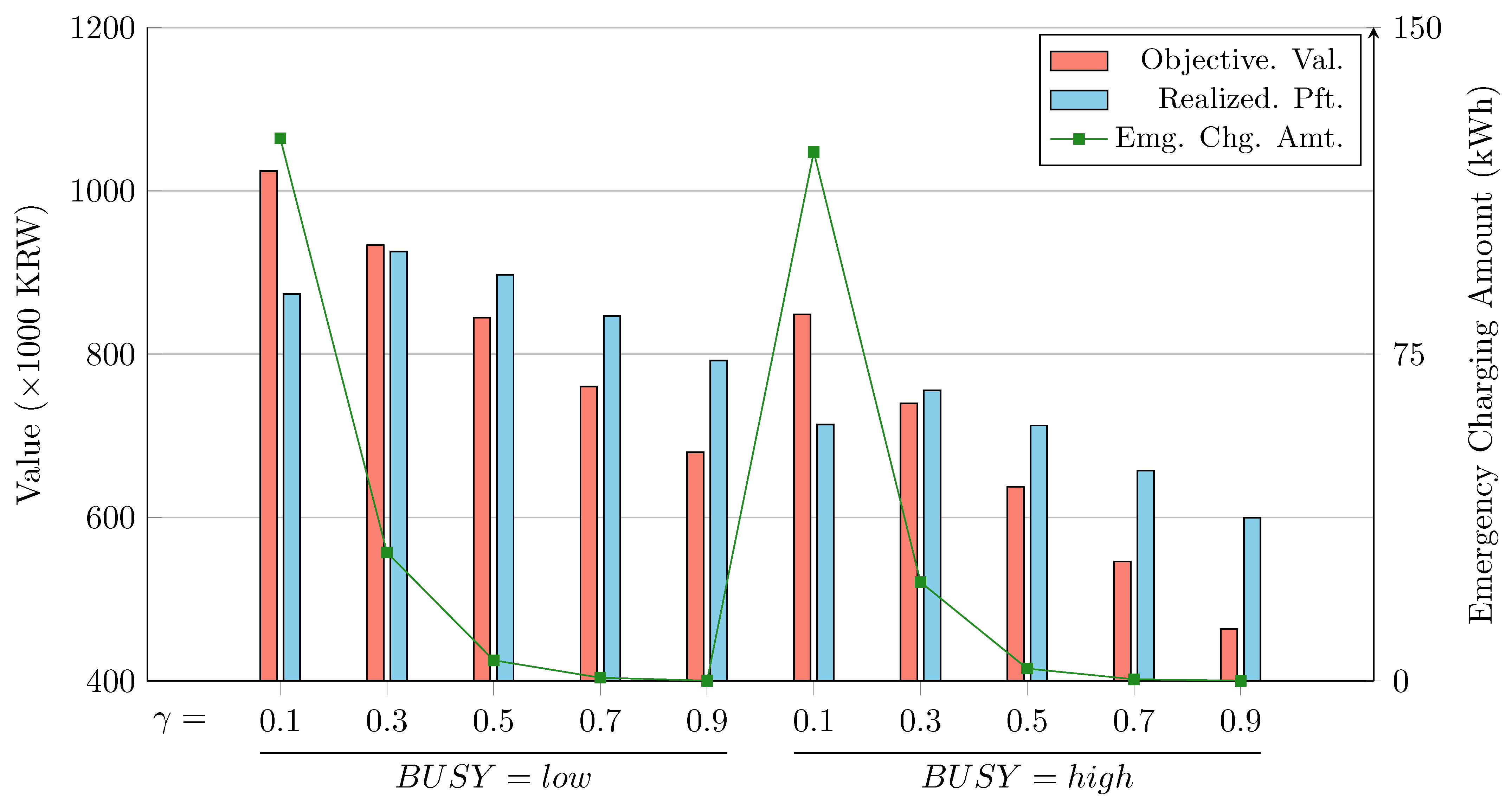
5.4. Impact of Budget Parameters

In this section, we analyze the impact of the budget parameters on the $R{O}_{budget}$ model by conducting experiments with varying $\gamma$ values. The value of $\gamma$ directly influences the budget parameters as ${\Gamma }_{ij}^c=\gamma ·j$ and ${\Gamma }_k^d=\gamma ·k$, determining the degree of conservatism in the model. As $\gamma$ increases, the uncertainty set expands, meaning that the $R{O}_{budget}$ model accounts for a greater level of uncertainty. The results are illustrated in Figure 10. The instance parameters are set as $NB=30$, $CR=low$, and $SEASON=summer$.

As expected, for the same instance settings, the objective value decreases as $\gamma$ increases. This is because a larger uncertainty set accounts for more scenarios, leading to a more conservative solution with a lower expected profit. However, the realized profit follows a different trend. The highest average realized profit is observed when $\gamma =0.3$, which coincides with the original uncertainty set’s coefficient of variation. This indicates that appropriately setting the budget parameter is crucial for maximizing profit. When $\gamma$ is too large, the model becomes overly conservative, leading to lower profit. Conversely, when $\gamma$ is too small, the budget is insufficient to account for uncertainty, resulting in solutions that lack robustness.

This trend is also reflected in the emergency charging amount. When $\gamma =0.1$, the emergency charging amount is significantly high, whereas as $\gamma$ increases, this amount drastically decreases. These results emphasize the importance of selecting an appropriate $\gamma$ value to effectively manage uncertainty and optimize the performance of the $R{O}_{budget}$ model.

6. Conclusions

This study addresses the charging and discharging scheduling problem for an E-bus depot equipped with V2G technology. To ensure feasible and cost-effective scheduling decisions under uncertainty, we proposed a robust optimization approach utilizing a budgeted uncertainty set. This approach allows for a controlled level of conservatism, ensuring robustness without overly sacrificing profitability.

The results of computational experiments validated the effectiveness of the proposed RO model. The results demonstrated that while the deterministic model achieved the highest objective value under nominal conditions, it performed poorly when uncertainty was realized, often leading to significant deviations in profit and increased emergency charging. In contrast, the proposed RO model with budgeted uncertainty set consistently outperformed both the deterministic and RO with box uncertainty set models in terms of realized profit, demonstrating its ability to balance robustness and profitability. The model also significantly reduced emergency charging, highlighting its practical viability. Sensitivity analyses on the budget parameter $\gamma$ revealed that setting an appropriate uncertainty budget is crucial. An excessively conservative budget reduced potential profit, while an insufficient budget failed to account for uncertainty effectively.

While this study provides a robust optimization framework for E-bus charging and discharging scheduling, several extensions can be explored to address more complex and realistic operational scenarios as future research directions. This study assumes a predetermined bus trip schedule. However, in practice, schedules may be flexible, requiring an integrated approach that simultaneously determines trip assignments and charging schedules for each bus. In addition, this study considers a single depot scenario, where all E-buses charge at the same location. In practice, transit networks may have multiple depots, and determining the charging location for each bus adds another layer of complexity. Extending the model to a multi-depot setting would be another interesting future research topics. Some E-bus depots may integrate renewable energy sources such as solar or wind power to supplement charging operations. Since the availability of these energy sources is uncertain, incorporating renewable generation uncertainty into the model could enhance its applicability in sustainable future transit systems.

While the proposed model incorporates a variety of operational constraints such as dual-port chargers, emergency charging, and load reduction requests, these features were included to reflect the complexity of real-world E-bus depot operations. Nevertheless, if certain features are not applicable to a specific depot, the corresponding constraints can be removed, resulting in a simplified version of the model. In particular, for large-scale instances, such simplifications can reduce computational complexity without significantly compromising solution quality. Exploring these simplified formulations is a promising direction for future research, especially in real-time or large-fleet applications where scalability is a critical concern.

Although we set the planning horizon to 22 h to reflect typical real-world E-bus depot operations, one can extend it beyond a single day to capture long-term operational patterns. This would allow for the analysis of cumulative uncertainty effects and battery degradation over time. Such an extension could provide further insights into the applicability of the proposed model in real-world depot operations.

This study focuses on an offline setting where all input data are assumed to be known in advance. In practice, however, operational decisions often need to be made in real-time due to unexpected delays, trip cancellations, or demand fluctuations. Developing a real-time or rolling-horizon scheduling framework that dynamically updates decisions as new information becomes available would further enhance the practical applicability of the model. Additionally, future research may consider incorporating driver scheduling constraints, such as maximum shift durations and break requirements. Accounting for such conditions would enable a more comprehensive and viable model that aligns more closely with actual workforce management policies in transit systems.

References

1. Requia, W.J.; Mohamed, M.; Higgins, C.D.; Arain, A.; Ferguson, M. How clean are electric vehicles? Evidence-based review of the effects of electric mobility on air pollutants, greenhouse gas emissions and human health. Atmos. Environ. 2018, 185, 64–77. [Google Scholar] [CrossRef]
2. International Energy Agency. Global EV Outlook 2024. Available online: https://www.iea.org/reports/global-ev-outlook-2024 (accessed on 20 April 2025).
3. Siemens. Siemens Technology Becoming Part of State-of-the-Art Bus Depot in Hamburg. Available online: https://press.siemens.com/global/en/pressrelease/siemens-technology-becoming-part-state-art-bus-depot-hamburg (accessed on 20 April 2025).
4. Tribune, Q. Lusail Bus Depot, One of the World’s Largest E-Bus Depot, Inaugurated. Available online: https://www.qatar-tribune.com/article/26042/latest-news/lusail-bus-depot-one-of-the-worlds-largest-e-bus-depot-inaugurated (accessed on 20 April 2025).
5. Ravi, S.S.; Aziz, M. Utilization of electric vehicles for vehicle-to-grid services: Progress and perspectives. Energies 2022, 15, 589. [Google Scholar] [CrossRef]
6. Mal, S.; Chattopadhyay, A.; Yang, A.; Gadh, R. Electric vehicle smart charging and vehicle-to-grid operation. Int. J. Parallel Emergent Distrib. Syst. 2013, 28, 249–265. [Google Scholar] [CrossRef]
7. Guille, C.; Gross, G. A conceptual framework for the vehicle-to-grid (V2G) implementation. Energy Policy 2009, 37, 4379–4390. [Google Scholar] [CrossRef]
8. Zhong, J.; He, L.; Li, C.; Cao, Y.; Wang, J.; Fang, B.; Zeng, L.; Xiao, G. Coordinated control for large-scale EV charging facilities and energy storage devices participating in frequency regulation. Appl. Energy 2014, 123, 253–262. [Google Scholar] [CrossRef]
9. Jian, L.; Zheng, Y.; Xiao, X.; Chan, C. Optimal scheduling for vehicle-to-grid operation with stochastic connection of plug-in electric vehicles to smart grid. Appl. Energy 2015, 146, 150–161. [Google Scholar] [CrossRef]
10. Pinson, P.; Madsen, H. Benefits and challenges of electrical demand response: A critical review. Renew. Sustain. Energy Rev. 2014, 39, 686–699. [Google Scholar]
11. Siano, P. Demand response and smart grids—A survey. Renew. Sustain. Energy Rev. 2014, 30, 461–478. [Google Scholar] [CrossRef]
12. Asamer, J.; Graser, A.; Heilmann, B.; Ruthmair, M. Sensitivity analysis for energy demand estimation of electric vehicles. Transp. Res. Part Transp. Environ. 2016, 46, 182–199. [Google Scholar] [CrossRef]
13. Pelletier, S.; Jabali, O.; Laporte, G. The electric vehicle routing problem with energy consumption uncertainty. Transp. Res. Part B Methodol. 2019, 126, 225–255. [Google Scholar] [CrossRef]
14. Jin, C.; Tang, J.; Ghosh, P. Optimizing electric vehicle charging: A customer’s perspective. IEEE Trans. Veh. Technol. 2013, 62, 2919–2927. [Google Scholar] [CrossRef]
15. García-Álvarez, J.; González, M.A.; Vela, C.R. Metaheuristics for solving a real-world electric vehicle charging scheduling problem. Appl. Soft Comput. 2018, 65, 292–306. [Google Scholar] [CrossRef]
16. Liu, J.; Lin, G.; Huang, S.; Zhou, Y.; Li, Y.; Rehtanz, C. Optimal EV charging scheduling by considering the limited number of chargers. IEEE Trans. Transp. Electrif. 2020, 7, 1112–1122. [Google Scholar] [CrossRef]
17. Honarmand, M.; Zakariazadeh, A.; Jadid, S. Optimal scheduling of electric vehicles in an intelligent parking lot considering vehicle-to-grid concept and battery condition. Energy 2014, 65, 572–579. [Google Scholar] [CrossRef]
18. Tan, M.; Ren, Y.; Pan, R.; Wang, L.; Chen, J. Fair and efficient electric vehicle charging scheduling optimization considering the maximum individual waiting time and operating cost. IEEE Trans. Veh. Technol. 2023, 72, 9808–9820. [Google Scholar] [CrossRef]
19. Seo, M.; Kodaira, D.; Jin, Y.; Son, H.; Han, S. Development of an efficient vehicle-to-grid method for massive electric vehicle aggregation. Energy Rep. 2024, 11, 1659–1674. [Google Scholar] [CrossRef]
20. He, Y.; Liu, Z.; Song, Z. Optimal charging scheduling and management for a fast-charging battery electric bus system. Transp. Res. Part E Logist. Transp. Rev. 2020, 142, 102056. [Google Scholar] [CrossRef]
21. Bagherinezhad, A.; Palomino, A.D.; Li, B.; Parvania, M. Spatio-temporal electric bus charging optimization with transit network constraints. IEEE Trans. Ind. Appl. 2020, 56, 5741–5749. [Google Scholar] [CrossRef]
22. Verbrugge, B.; Rauf, A.M.; Rasool, H.; Abdel-Monem, M.; Geury, T.; El Baghdadi, M.; Hegazy, O. Real-time charging scheduling and optimization of electric buses in a depot. Energies 2022, 15, 5023. [Google Scholar] [CrossRef]
23. Bao, Z.; Li, J.; Bai, X.; Xie, C.; Chen, Z.; Xu, M.; Shang, W.L.; Li, H. An optimal charging scheduling model and algorithm for electric buses. Appl. Energy 2023, 332, 120512. [Google Scholar] [CrossRef]
24. Huang, D.; Wang, Y.; Jia, S.; Liu, Z.; Wang, S. A Lagrangian relaxation approach for the electric bus charging scheduling optimisation problem. Transp. A Transp. Sci. 2023, 19, 2023690. [Google Scholar] [CrossRef]
25. Zhou, Y.; Meng, Q.; Ong, G.P.; Wang, H. Electric bus charging scheduling on a bus network. Transp. Res. Part C Emerg. Technol. 2024, 161, 104553. [Google Scholar] [CrossRef]
26. Zhou, Y.; Wang, H.; Wang, Y.; Yu, B.; Tang, T. Charging facility planning and scheduling problems for battery electric bus systems: A comprehensive review. Transp. Res. Part E Logist. Transp. Rev. 2024, 183, 103463. [Google Scholar] [CrossRef]
27. Noel, L.; McCormack, R. A cost benefit analysis of a V2G-capable electric school bus compared to a traditional diesel school bus. Appl. Energy 2014, 126, 246–255. [Google Scholar] [CrossRef]
28. Arif, S.M.; Lie, T.T.; Seet, B.C.; Ahsan, S.M.; Khan, H.A. Plug-in electric bus depot charging with PV and ESS and their impact on LV feeder. Energies 2020, 13, 2139. [Google Scholar] [CrossRef]
29. Rafique, S.; Nizami, M.; Irshad, U.; Hossain, M.; Mukhopadhyay, S. A two-stage multi-objective stochastic optimization strategy to minimize cost for electric bus depot operators. J. Clean. Prod. 2022, 332, 129856. [Google Scholar] [CrossRef]
30. Bertsimas, D.; Brown, D.B.; Caramanis, C. Theory and applications of robust optimization. SIAM Rev. 2011, 53, 464–501. [Google Scholar] [CrossRef]
31. Yao, Z.; Wang, Z.; Ran, L. Smart charging and discharging of electric vehicles based on multi-objective robust optimization in smart cities. Appl. Energy 2023, 343, 121185. [Google Scholar] [CrossRef]
32. Jiang, M.; Zhang, Y.; Zhang, Y. Optimal electric bus scheduling under travel time uncertainty: A robust model and solution method. J. Adv. Transp. 2021, 2021, 1191443. [Google Scholar] [CrossRef]
33. Zhou, Y.; Wang, H.; Wang, Y.; Li, R. Robust optimization for integrated planning of electric-bus charger deployment and charging scheduling. Transp. Res. Part D Transp. Environ. 2022, 110, 103410. [Google Scholar] [CrossRef]
34. Shi, R.; Li, S.; Zhang, P.; Lee, K.Y. Integration of renewable energy sources and electric vehicles in V2G network with adjustable robust optimization. Renew. Energy 2020, 153, 1067–1080. [Google Scholar] [CrossRef]
35. Jiao, Z.; Ran, L.; Zhang, Y.; Ren, Y. Robust vehicle-to-grid power dispatching operations amid sociotechnical complexities. Appl. Energy 2021, 281, 115912. [Google Scholar] [CrossRef]
36. Hao, L.; Wang, Y.Y.; Gopalakrishnan, S.; Namuduri, C.S.; Prasad, R.; Raghavan, M. Adaptive Fast-Charging of Multi-Pack Battery System in a Mobile Platform Having Dual Charge Ports. US Patent 11,336,101, 17 May 2022. [Google Scholar]
37. Soyster, A.L. Convex programming with set-inclusive constraints and applications to inexact linear programming. Oper. Res. 1973, 21, 1154–1157. [Google Scholar] [CrossRef]
38. Bertsimas, D.; Sim, M. The price of robustness. Oper. Res. 2004, 52, 35–53. [Google Scholar] [CrossRef]
39. Bertsimas, D.; Thiele, A. A robust optimization approach to inventory theory. Oper. Res. 2006, 54, 150–168. [Google Scholar] [CrossRef]
40. Al-Ogaili, A.S.; Al-Shetwi, A.Q.; Al-Masri, H.M.; Babu, T.S.; Hoon, Y.; Alzaareer, K.; Babu, N.P. Review of the estimation methods of energy consumption for battery electric buses. Energies 2021, 14, 7578. [Google Scholar] [CrossRef]
41. Rachna; Singh, A.K. Analyzing electric vehicle performance considering smooth roads with seasonal variation. Electr. Eng. 2024, 107, 3709–3723. [Google Scholar] [CrossRef]
Figure 1. Notation regarding time periods and peak hours.
Mathematics 13 01380 g001
Figure 2. Dual-port charging system of GM. (This figure is adopted from [36]. For the description of the numbered components, please refer to the cited patent.)
Mathematics 13 01380 g002
Figure 3. E-bus trip schedule table.
Mathematics 13 01380 g003
Figure 4. Energy consumption by season and passenger load.
Mathematics 13 01380 g004
Figure 5. Time-of-Use (TOU) price.
Mathematics 13 01380 g005
Figure 6. Comparison of objective function value of optimization models and realized profits.
Mathematics 13 01380 g006
Figure 7. Distribution of realized profits for 500 scenarios.
Mathematics 13 01380 g007
Figure 8. Distribution of emergency charging amounts for 500 scenarios.
Mathematics 13 01380 g008
Figure 9. Out-of-sample experiment results.
Mathematics 13 01380 g009
Figure 10. Impact of budget parameter γ .
Mathematics 13 01380 g010