Article

Improving the Reliability of Parallel and Series–Parallel Systems by Reverse Engineering of Algebraic Inequalities

School of Engineering, Computing and Mathematics, Oxford Brookes University, Oxford OX3 0BP, UK
Mathematics 2025, 13(9), 1381; https://doi.org/10.3390/math13091381
Submission received: 18 March 2025 / Revised: 17 April 2025 / Accepted: 18 April 2025 / Published: 24 April 2025

Abstract

:
This paper presents a novel, domain-independent method for enhancing system reliability based on reverse engineering of algebraic inequalities. Although system reliability has been extensively studied, existing approaches have not addressed the challenge of improving reliability without knowing the reliability of individual components. This work fills this gap by demonstrating that the reliability of both parallel and series–parallel systems can be improved without any information about component reliability values. Specifically, this study establishes that in parallel systems, a symmetric arrangement of interchangeable components of the same type across parallel branches consistently yields higher system reliability than an asymmetric arrangement—regardless of the individual component reliabilities. This finding is derived through the reverse engineering of a new general algebraic inequality, proposed and proved for the first time. Furthermore, applying the same approach to series–parallel systems reveals that asymmetric arrangements of interchangeable redundancies offer superior system reliability compared with symmetric configurations.

1. Introduction

Standard textbooks on reliability engineering and system reliability [1,2,3,4,5,6,7,8,9,10,11] do not address a fundamental question related to how to improve system reliability without requiring specific knowledge of individual component reliabilities. Even components of the same type exhibit significant uncertainty in reliability due to factors such as manufacturer, age, operating environment, and duty cycle. For example, sensors of the same type sourced from different suppliers can show considerable reliability variations because of the different variety. Information about the reliability of different component varieties from suppliers is often missing, difficult to obtain, or highly unreliable. Therefore, it is crucial to develop methods for enhancing system reliability without relying on any knowledge of the reliabilities of individual components of different varieties.
Despite the extensive research on redundancy optimisation in the reliability literature, existing techniques universally assume prior knowledge of component reliabilities. However, no method has yet addressed redundancy optimisation in the absence of this information. Traditional approaches to optimal redundancy allocation begin with known reliability values for all components and redundant units. For instance, a multi-performance redundancy optimisation technique for multi-state systems based on genetic algorithms and relying explicitly on known component reliabilities was proposed in [12]. Similarly, Ref. [13] tackled the redundancy allocation problem by using nature-inspired AI algorithms, such as adaptive particle swarm optimisation, which also requires the availability of component reliability data.
To tackle redundancy allocation in large-scale systems, several methods have been proposed in [14], including the Lagrange multipliers technique, a pairwise hill-climbing algorithm, and an evolutionary algorithm. Furthermore, Ref. [15] provides a review of system reliability optimisation techniques based on importance measures, all of which similarly rely on known component reliabilities.
For a long time, algebraic inequalities have been employed for estimating upper and lower bounds, quantifying errors, and defining design constraints in engineering applications [16,17,18,19,20,21,22,23,24,25,26,27,28,29,30,31]. Traditionally, these inequalities have served as analytical tools. However, a fundamental shift in their application has emerged with the concept of reverse engineering of algebraic inequalities—a novel approach that leverages algebraic inequalities to generate new knowledge and optimise engineering systems and processes [32].
The reverse engineering of algebraic inequalities begins with a mathematically valid inequality and interprets it within a physical or engineering context. When the variables and terms in such an inequality correspond to controlling factors or attributes of a physical system or process, the system exhibits behaviours consistent with the inequality’s predictions [32]. In this way, reverse engineering can reveal new insights or even uncover previously unrecognised physical principles.
Through this process, valid algebraic inequalities become tools for discovering new relationships and enhancing the performance of systems—without the need for prior data. The knowledge generated can be applied to optimise design, improve reliability, and guide decision making.
The key novel contributions of this paper are as follows:
  • The proposal and proof of a new general algebraic inequality, applicable to enhancing the reliability of parallel and series–parallel systems.
  • The development of a method to improve the reliability of parallel and series–parallel systems through the reverse engineering of complex algebraic inequalities—without requiring any information about the reliability of individual components.
  • The establishment of a foundational result: for parallel systems, a symmetric arrangement of interchangeable components across parallel branches consistently yields higher reliability than an asymmetric arrangement, regardless of the components’ individual reliabilities or their rankings.
  • The establishment of another foundational result: for series–parallel systems, an asymmetric arrangement of interchangeable redundant components consistently yields higher reliability than a symmetric arrangement, regardless of the components’ individual reliabilities or their rankings.

2. Improving System Reliability of Parallel Systems Through Symmetric Arrangement of Components

In what follows, applications related to improving the reliability of common parallel systems with interchangeable components of the same type but of different varieties will be proposed.
The reliability improvement method is low-cost and domain-independent, and can be used for improving reliability and reducing the risk of failure in various unrelated domains.
This method is derived from the reverse engineering of the algebraic inequality
( 1 r 1 2 ) ( 1 r 2 2 ) ( 1 r m 2 ) ( 1 r 1 r 2 ) ( 1 r 2 r 3 ) ( 1 r m r 1 ) 0 r i 1 ,
where r i are variable accepting values from the interval [0, 1].
Inequality (1) is a special case of inequality (7) whose proof has been presented in the Appendix A.
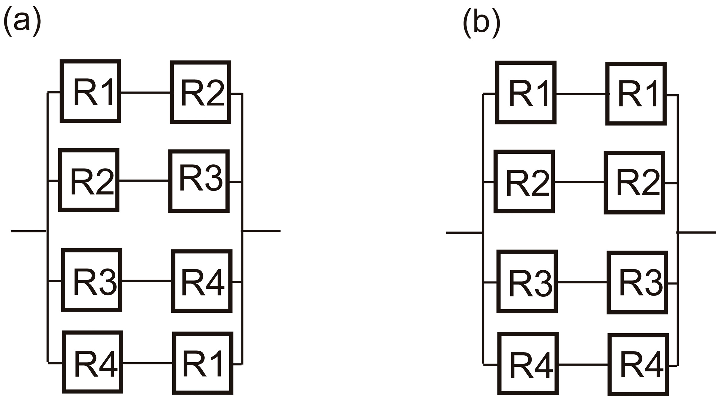
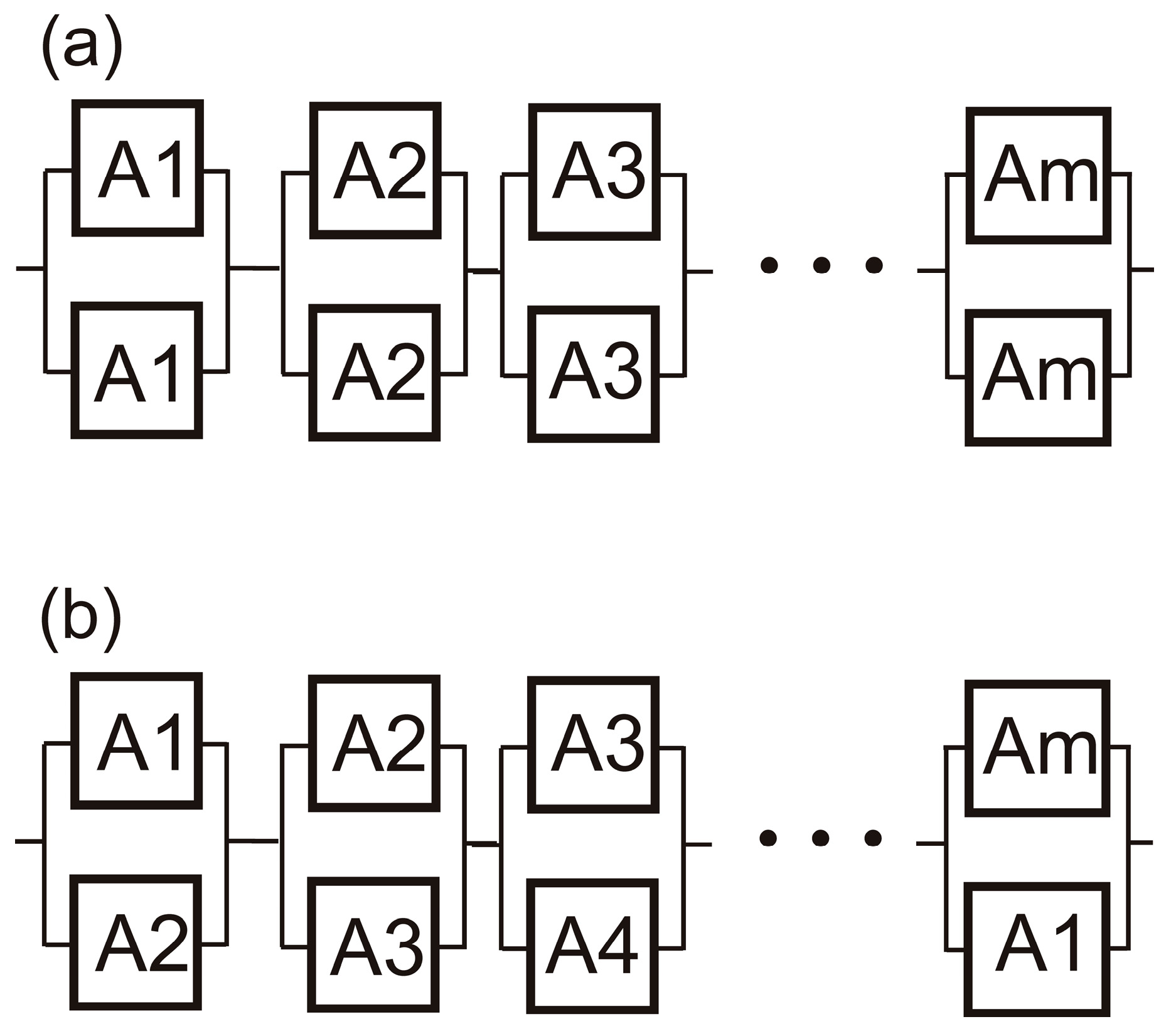
Now, let r i , i = 1 , , m in (1) be physically interpreted as the ‘reliabilities’ of components working independently from one another, from varieties R i ( i = 1 , , m ) (Figure 1). Let us suppose that all components are of the same type (e.g., type ‘seals’) but of different variety (e.g., from a different manufacturer).
The reverse engineering of Inequality (1) reveals that its left-hand side can be interpreted as the probability of system failure F b = ( 1 r 1 2 ) ( 1 r 2 2 ) ( 1 r 3 2 ) ( 1 r m 2 ) for the configuration shown in Figure 1b, while its right-hand side corresponds to the probability of failure F a = ( 1 r 1 r 2 ) ( 1 r 2 r 3 ) ( 1 r 3 r 4 ) ( 1 r m r 1 ) for the system depicted in Figure 1a. Indeed, the systems in Figure 1 are in a working state if at least one of the parallel branches is in a working state. The systems are in a failed state when all parallel branches are in a failed state. Therefore, the probability of failure of the parallel systems in Figure 1 is equal to the product of the probabilities of failure of every single parallel branch in the systems, which yields the expressions F a = ( 1 r 1 r 2 ) ( 1 r 2 r 3 ) ( 1 r 3 r 4 ) ( 1 r m r 1 ) and F b = ( 1 r 1 2 ) ( 1 r 2 2 ) ( 1 r 3 2 ) ( 1 r m 2 ) for the probabilities of failure of the systems in Figure 1a,b.
The reverse engineering of Inequality (1) effectively establishes that the symmetric arrangement of interchangeable components of the same variety in each parallel branch (Figure 1b) is always characterised by a smaller probability of system failure, compared with their asymmetric arrangement (Figure 1a), irrespective of the reliabilities r i of the components.
Note that even though the reliabilities r i of component varieties and their rankings are unknown, the reliability of the system in Figure 1a, which has an asymmetrical arrangement of the component varieties, can still be enhanced by introducing a symmetric arrangement of the component varieties (Figure 1b). To improve the system’s reliability, there is no need to know the reliabilities of the different varieties or their ranking according to their reliability.
We must point out that no particular ranking of the component varieties by their reliability is necessary for the method to be applied. To demonstrate this, we select the parallel systems in Figure 2 consisting of four branches connected in parallel.
The reliabilities of the component varieties and the probabilities of failure of the systems in (a) and (b) are given in Table 1. The values r 1 , r 2 , r 3 , and r 4 correspond to the reliabilities of the component varieties R 1 , R 2 , R 3 , and R 4 in Figure 2. The values F a = ( 1 r 1 r 2 ) ( 1 r 2 r 3 ) ( 1 r 3 r 4 ) ( 1 r 4 r 1 ) are the probabilities of failure of the systems with an asymmetric arrangement of the component varieties (Figure 2a), while the values F b = ( 1 r 1 2 ) ( 1 r 2 2 ) ( 1 r 3 2 ) ( 1 r 4 2 ) are the probabilities of failure of the system with a symmetric arrangement of the interchangeable component varieties (Figure 2b).
As evidenced by Table 1, in all permutations of component reliabilities, the symmetric arrangement of component varieties across the parallel branches consistently results in a lower probability of system failure ( F b < F a ). This trend holds universally, with no exceptions observed—even if the table were extended indefinitely.
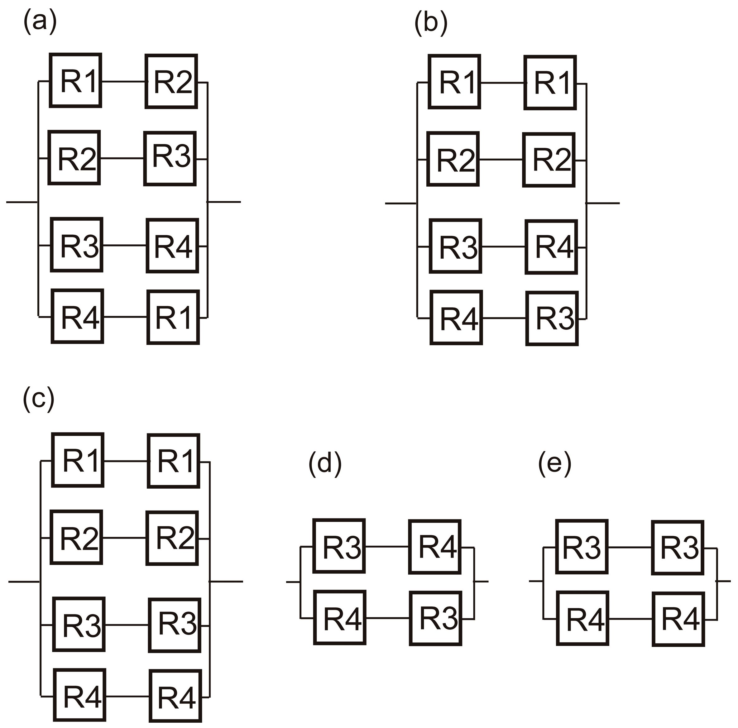
To maximise the reliability of the original system under conditions of complete uncertainty regarding the reliabilities of individual components, the system’s configuration must eliminate all asymmetries throughout its structure. Let us consider the system shown in Figure 3a. Its reliability can be improved by making the arrangement of component varieties symmetrical, in the first and second branches, resulting in the modified system depicted in Figure 3b.
However, further improvements can be achieved by eliminating the remaining asymmetries in the third and fourth parallel branches. This leads to the fully symmetric configuration illustrated in Figure 3c. The system in Figure 3c is more reliable than the one in Figure 3b for the following reasons:
  • In Figure 3b, the section shown in Figure 3d is connected in parallel within the system, whereas in Figure 3c, the corresponding section is that shown in Figure 3e.
  • The section in Figure 3d exhibits a higher probability of failure compared with the symmetrical and more reliable section in Figure 3e.
Interchangeable components may encompass various types that align with real-world applications. For instance, interchangeable temperature gauges can operate based on different physical principles—such as thermocouples, radiation thermometers, thermal resistors, or bi-metal thermometers. Similarly, a wide range of options exist for measuring other parameters, like pressure, concentration, and more. Moreover, even within a single component type, variations in component reliability can arise depending on the manufacturer and the age of the components.
It needs to be clarified that the interchangeable component varieties and types can be characterised with distinct failure modes and these do not restrict the application of the proposed method. The distinct failure modes (e.g., wear-out failures and overstress failures) affect only the time to failure of the components and their reliability values.

Application Examples Related to Improving Reliability of Parallel Systems

An example of a mechanical system that can benefit from a symmetric rearrangement of components of the same variety in the parallel branches is given in Figure 4. The system consists of three parallel lines transporting cooling fluid from sources s1, s2, and s3 to a chemical reactor CR with two pumping sections on each parallel line.
The system is deemed operational if at least one of the parallel branches is operational and delivers cooling fluid to the chemical reactor. The interchangeable pumping sections are of varieties R1 (a pumping section from manufacturer 1), R2 (a pumping station from manufacturer 2), and R3 (a pumping station from manufacturer 3), characterised by unknown reliabilities r 1 , r 2 , r 3 , respectively.
The reliability network of the systems in Figure 4a,b are given in Figure 1a,b, respectively, for m = 3 parallel branches. These parallel systems are quite common in numerous engineering applications.
The proposed reliability improvement technique exploiting the reverse engineering of Inequality (1) is domain-independent. It can be used for any parallel system with interchangeable components: valves, sensors, seals, etc.
In another example, Figure 5 presents a system that can also benefit from a symmetric arrangement of interchangeable sensors in the parallel branches.
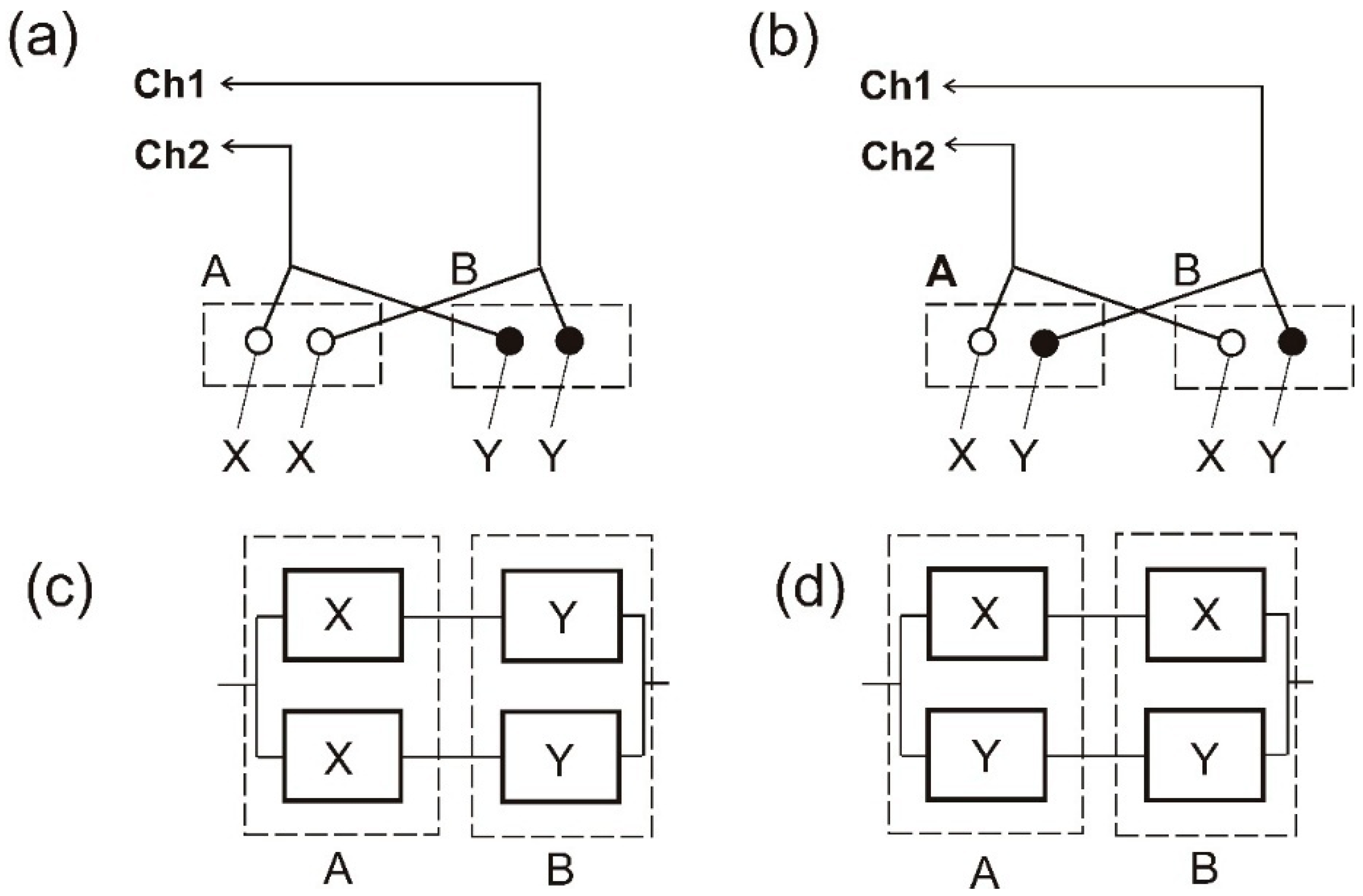
This system comprises two zones, A and B, where the temperature (pressure, concentration, etc.) is measured in each zone by interchangeable sensors of varieties X and Y. To enhance the system’s reliability, two parallel measurement channels, Ch1 and Ch2, have been introduced, each measuring the difference in temperature/pressure/concentration between the two zones (Figure 5a). To guarantee operational safety, at least one of the channels must provide a valid measurement from each zone. Channel redundancy ensures that a valid measurement of the temperature difference between the two zones will still be made even if any of the sensors fails.
The sensors are of varieties X and Y, characterised by unknown reliabilities r 1 and r 2 , respectively. The reliability networks of the systems in Figure 5a,b are given in Figure 5c,d, respectively. These are also parallel systems with interchangeable components. For m = 2 , Inequality (1) transforms into the special-case inequality
( 1 r 1 2 ) ( 1 r 2 2 ) ( 1 r 1 r 2 ) ( 1 r 2 r 1 ) 0 r i 1
The left-hand side, F b = ( 1 r 1 2 ) ( 1 r 2 2 ) , of Inequality (2) can be physically interpreted as the probability of failure F b of the system in Figure 5b, while the right-hand side, F a = ( 1 r 1 r 2 ) ( 1 r 2 r 1 ) , of Inequality (2) can be physically interpreted as the probability of failure F a of the system in Figure 5a.
According to Inequality (2), the probability of failure for the system with the same variety of sensors in each channel (Figure 5b) is smaller than the probability of failure of the system with different varieties of sensors in each channel (Figure 5a) ( F b F a ).
The difference in the probabilities of failure of the systems in Figure 5a,b can be significant, as the next numerical examples demonstrate.
Let us suppose that for a given period of operation, the reliabilities r 1 and r 2 of the sensor varieties are those in Table 2. The table also lists the probabilities of failure F a = ( 1 r 1 r 2 ) ( 1 r 2 r 1 ) and F b = ( 1 r 1 2 ) ( 1 r 2 2 ) of the systems in Figure 5a,b. The probabilities of failure of the systems in Figure 5a are significantly greater than the probabilities of failure of the systems in Figure 5b. The symmetric configuration of the sensor varieties in Figure 5b leads to a dramatic improvement in the system’s reliability. Table 2 summarises these results.

3. Parallel Systems with Multiple Components in Each Branch

The reverse engineering of algebraic inequalities can also enhance the reliability of parallel systems composed of multiple components per branch, particularly when the reliabilities of individual components are unknown. It is assumed that each parallel branch in the system contains the same number of interchangeable components.
Let us consider the correct abstract algebraic inequality
( 1 x 3 ) ( 1 y 3 ) ( 1 z 3 ) ( 1 x 2 y ) ( 1 y 2 z ) ( 1 z 2 x )
which is a special case of the general inequality (7), rigorously proved in the Appendix A. In Inequality (3): 0 x 1 , 0 y 1 , and 0 z 1 .
Let the variables x, y, and z in Inequality (3) represent the reliabilities of components of types X, Y, and Z, respectively. In this context, the left-hand and right-hand sides of Inequality (3) can be interpreted as the probabilities of failure for two alternative parallel systems. To illustrate this interpretation, let us consider the physical configurations depicted in Figure 6. Each system comprises three parallel gas lines, where each line consists of pumping sections of types X, Y, and Z, connected in series. The entire system operates successfully if at least one gas line can deliver gas to the consumer, C.
The gas lines in the system in Figure 6a have an asymmetric arrangement of the types of pumping stations, while the gas lines in the system in Figure 6b have a symmetric arrangement of the types of pumping stations.
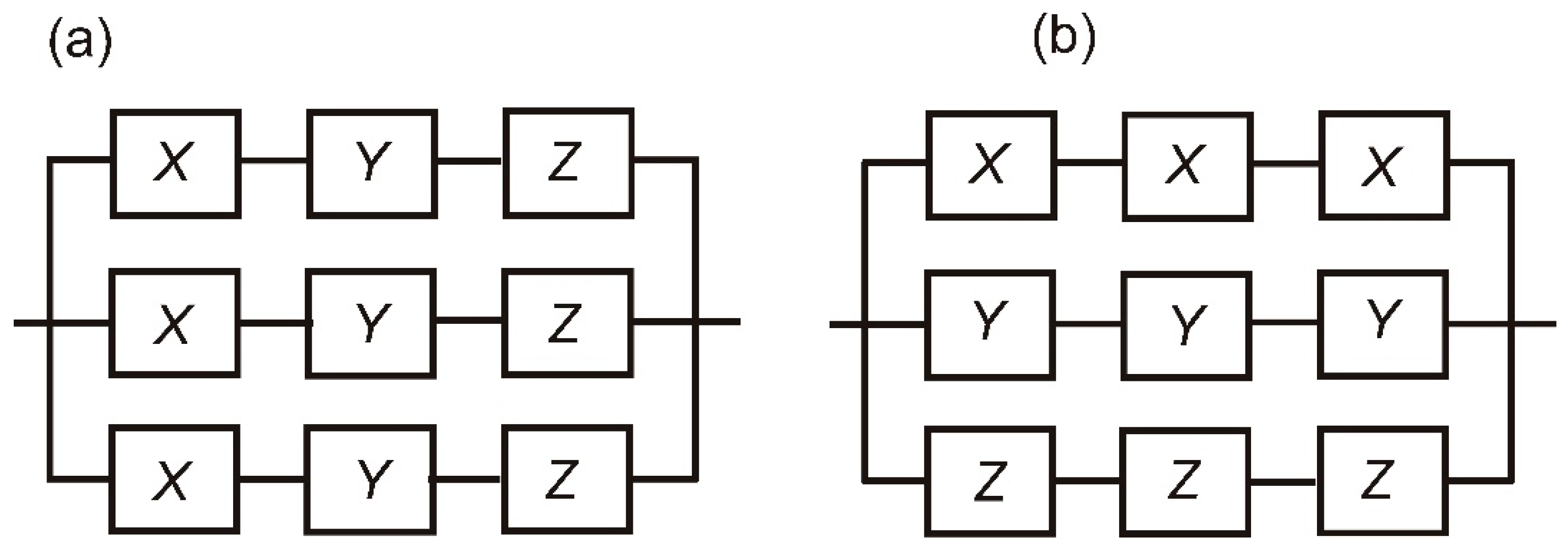
In relation to fluid delivery to consumer C, the reliability networks associated with the physical setups in Figure 6a,b are shown in Figure 7a and Figure 7b, respectively. These networks illustrate the logical arrangement of the system’s components.
If the reliabilities of the section types X, Y, and Z are represented by x, y, and z, respectively ( 0 x 1 , 0 y 1 , and 0 z 1 ), then the probability of failure F b of the system in Figure 6b is expressed by F b = ( 1 x 3 ) ( 1 y 3 ) ( 1 z 3 ) , whereas the probability of failure F a for the system in Figure 6a is given by F a = ( 1 x 2 y ) ( 1 y 2 z ) ( 1 z 2 x ) . The reliabilities x, y, and z, of the pumping sections and their rankings are unknown.
By reverse-engineering Inequality (3), it can be inferred that the left-hand side corresponds to the probability of failure for the system shown in Figure 6b, while the right-hand side reflects the probability of failure for the system in Figure 6a.
As stated in Inequality (3), the system depicted in Figure 6b exhibits higher reliability than the one in Figure 6a. This conclusion is drawn without any prior knowledge of the failure probabilities x, y, and z for the three distinct section types or of their relative ranking.
Inequalities similar to Inequality (3) can be reverse-engineered relatively easily because products of the type ( 1 r 1 n ) ( 1 r 2 n ) ( 1 r m n ) , where r i is the reliability of component of type i, can be interpreted directly as the probability of failure of a parallel system with m parallel branches and n components in each branch.
In this connection, Inequalities (4)–(6), where 0 x , y , z 1 , can be proved rigorously, as special cases of a general inequality proved in the Appendix A. Inequalities (4)–(6) can also be reverse-engineered as ‘probabilities of failure of parallel systems with multiple interchangeable components’.
( 1 x 3 ) ( 1 y 3 ) ( 1 z 3 ) ( 1 x y z ) ( 1 y z x ) ( 1 z x y )
( 1 x 4 ) ( 1 y 4 ) ( 1 z 4 ) ( 1 x 2 y 2 ) ( 1 y 2 z 2 ) ( 1 z 2 x 2 )
( 1 x 4 ) ( 1 y 4 ) ( 1 z 4 ) ( 1 x 2 y z ) ( 1 y 2 z x ) ( 1 z 2 x y )
By interpreting x, y, and z as the reliabilities of components from varieties X, Y, and Z, respectively, the reverse engineering of Inequalities (4)–(6) reveals that their left- and right-hand sides represent the probabilities of failure of the parallel systems depicted in Figure 8, Figure 9 and Figure 10. Specifically, the left-hand sides correspond to the reliability of the systems in Figure 8b, Figure 9b, and Figure 10b, respectively, while the right-hand sides correspond to the reliability of the systems in Figure 8a, Figure 9a, and Figure 10a, respectively.
The reliability improvement technique obtained for parallel systems with an equal number of components in each parallel branch cannot be automatically extrapolated to systems with a different number of components in each parallel branch because systems with a different number of components in each branch are no longer symmetrical. If, for systems with an unequal number of components in each branch, inequalities similar to Inequalities (3)–(6) can be proved to be correct, then symmetric arrangements of components will result in a system reliability improvement.

4. A General Inequality

Inequalities (1), (3)–(6) can be generalized for a network consisting of m types of components, arranged in m parallel branches, with n components in each branch
Let us suppose that 0 x 1 , x 2 , x m 1 are the reliabilities of the components of each of the m types. Then, it can be shown that the inequality holds,
( 1 x 1 n ) ( 1 x 2 n ) ( 1 x m n ) ( 1 c 11 c 21 c n 1 ) ( 1 c 12 c 22 c n 2 ) ( 1 c 1 m c 2 m c n m )
where c i j 0 denotes the reliability of the ith component in the jth parallel branch of the network (i = 1, …, n; j = 1, …, m). The terms f 1 = ( 1 c 11 c 21 c n 1 ) ,   f 2 = ( 1 c 12 c 22 c n 2 ) , , f m = ( 1 c 1 m c 2 m c n m ) give the probabilities of failure f i (i = 1, …, n) of the parallel branches of the network which reflects the right-hand side of Inequality (7). Any of the c i j 0 in the right-hand side of Inequality (7) stands for the reliability of the ith component in the jth parallel branch, and is equal to one of the values x 1 , x 2 , , x m , characterising the reliabilities of the m different types of components. In addition, the sum of the numbers of components from each type in the network must be the same, equal to the number n of components in a parallel branch. The proof of the inequality (7) has been presented in the Appendix A.
As can be verified, Inequality (1) is a special case of inequality (7), for m different component types, m parallel branches and n = 2 components in each parallel branch. Inequalities (3) and (4) are special cases of inequality (7), for m = 3 different types of components, m = 3 parallel branches and n = 3 components in a parallel branch. Inequalities (5) and (6) are also special cases of Inequality (7), for m = 3 different types of components, m = 3 parallel branches and n = 4 components in each parallel branch.
It is important to emphasise that the selection of the number of branches cannot be made independently of the number of types of components, because the number of branches must be equal to the number of component types.
Note that each parallel branch must contain the same number of components. Speculative extensions of these results—such as using a different number of components in different branches or a number of branches that differs from the number of component types—cannot be made without first rigorously proving an inequality whose reverse engineering reflects such a scenario.

5. Alternative Interpretation of Inequality (1)

Interestingly, Inequality (1) can also be reverse-engineered to represent series–parallel systems (Figure 11a) if the variables in the inequality are interpreted not as reliabilities but as probabilities of failure.
Let us rewrite Inequality (1) in the following form:
( 1 f 1 2 ) ( 1 f 2 2 ) ( 1 f m 2 ) ( 1 f 1 f 2 ) ( 1 f 2 f 3 ) ( 1 f m f 1 ) 0 f i 1
where f i are variables accepting values from the interval [0, 1].
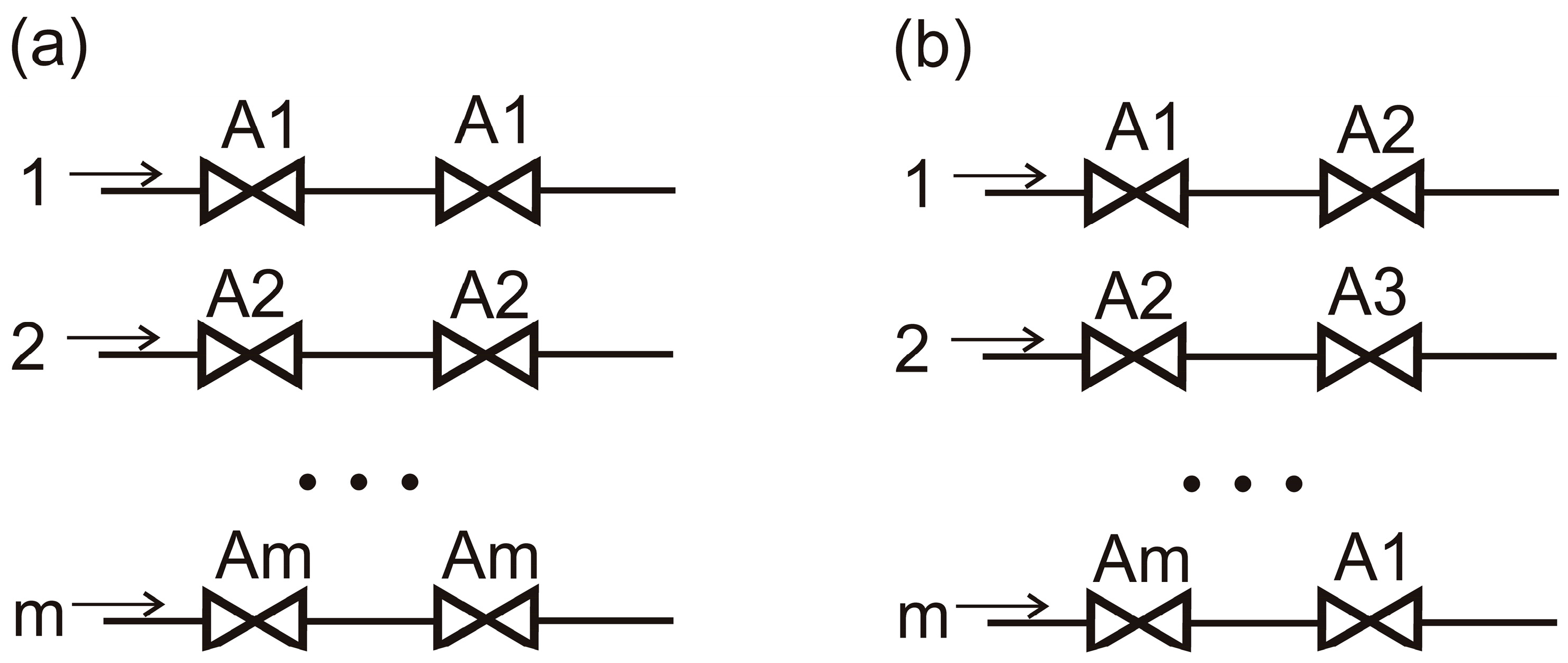
Now, let f i , i = 1 , , m in (8) be physically interpreted as ‘probabilities of failure’ of components of type A i ( i = 1 , , m ). The reverse engineering of Inequality (8) then yields that the left-hand side of the inequality can be physically interpreted as the reliability R a = ( 1 f 1 2 ) ( 1 f 2 2 ) ( 1 f 3 2 ) ( 1 f m 2 ) of the system in Figure 11a, while the right-hand side of the inequality R b = ( 1 f 1 f 2 ) ( 1 f 2 f 3 ) ( 1 f 3 f 4 ) ( 1 f m f 1 ) can be physically interpreted as the reliability of the system in Figure 11b.
Inequality (8) effectively establishes the opposite of what has been established for parallel systems: the asymmetric arrangement of the interchangeable redundancies is now characterised by a larger reliability, compared with their symmetric arrangement, irrespective of the probabilities of failure f i of the components.
Note that even though the probabilities of failure f i of components and their rankings are unknown, the reliability of the system in Figure 11a, which has a symmetrical arrangement of the redundant components, can still be enhanced by introducing an asymmetric arrangement of redundancies. To improve the system’s reliability, there is no need to know the probabilities of failure or the ranking of the components by their probability of failure.
To demonstrate this, we select the series–parallel system in Figure 11 consisting of four sections connected in series (m = 4).
The probabilities of failure of the components and the reliabilities of the systems in (a) and (b) are given in Table 3. The values f 1 , f 2 , f 3 , and f 4 correspond to the probabilities of failure of the components A 1 , A 2 , A 3 and A 4 in Figure 11 (m = 4). The values R a = ( 1 f 1 2 ) ( 1 f 2 2 ) ( 1 f 3 2 ) ( 1 f 4 2 ) are the reliabilities of the systems with symmetric redundancies, while the values R b = ( 1 f 1 f 2 ) ( 1 f 2 f 3 ) ( 1 f 3 f 4 ) ( 1 f 4 f 1 ) are the reliabilities of the systems with asymmetric redundancies.
As evidenced by Table 3, in every instance of ordering the component reliabilities, the asymmetric arrangement of redundancies consistently results in a system with superior reliability ( R b > R a ). This trend holds without exception and will continue to do so even if the table is extended indefinitely.
An example of a mechanical series–parallel system that benefits from an asymmetric arrangement of redundancies is illustrated in Figure 12. The system comprises n pipelines transporting toxic fluid, each equipped with two valves. Initially, all valves are open. To stop the flow in each pipeline, a closure signal is simultaneously sent to all valves.
The system is considered operational if, upon receiving the closure command, the flow is successfully halted in all n pipelines. To improve reliability, each pipeline includes a redundant valve—meaning that at least one of the two valves on each pipeline must respond to the closure signal to stop the flow in the pipeline.
The valves are of types A1, A2, …, Am, characterised by probabilities of failure to close on demand f 1 , f 2 , , f m , respectively.

6. Conclusions

6.1. Summary of Findings

-
The reliability of parallel and series–parallel systems can be enhanced without the need to know the reliabilities of individual components.
-
A new general algebraic inequality related to the reliability of parallel and series-parallel systems has been proposed and proved for the first time.
-
A novel, algorithmic proof technique has been developed to establish the proposed general inequality
-
Through the reverse engineering of the new general inequality, it was discovered that symmetric arrangements of identical, interchangeable components in parallel systems result in higher reliability compared with asymmetric configurations.
-
For series–parallel systems, asymmetric arrangements of interchangeable redundancies lead to greater system reliability than symmetric ones.

6.2. Significance of Results

Although system reliability has been extensively studied, existing approaches have not addressed the challenge of improving reliability without knowing the reliability of individual components. This work fills that gap by demonstrating that the reliability of both parallel and series–parallel systems can be improved without any information about component reliability values. Additionally, the proposed technique incurs no implementation costs and can be applied to improve the reliability of parallel and series-parallel systems, thereby reducing the risk of failure across various unrelated fields.

6.3. Limitations of This Study

Speculative extensions of the presented results—such as using a different number of components in the parallel branches or a number of branches that differs from the number of component types—cannot be made without first rigorously proving an inequality whose reverse engineering reflects such a scenario.

6.4. Suggestions for Future Research

This study can be extended by proposing and proving inequalities related to the reliability of parallel systems with different number of components in the parallel branches.

Funding

This research study received no external funding.

Data Availability Statement

The original contributions presented in this study are included in the article. Further inquiries can be directed to the author.

Conflicts of Interest

The author declares no conflicts of interest.

Appendix A

Proof of the general inequality (7). 
The truth of inequality (7) will be established by an algorithmic proof. Let us assume that the variables 0 < x 1 , x 2 , , x m < 1 in the inequality are distinct. Without loss of generality, these variables can be assumed to be arranges in descending order of their values: 1 > x 1 > x 2 > , > x m > 0 . Any of the variables c i j 0 in the right-hand side of Inequality (7) has a value equal to the value of one of the x 1 , x 2 , , x m variables. Without loss of generality, the m terms:
f 1 = ( 1 c 11 c 21 c n 1 ) , f 2 = ( 1 c 12 c 22 c n 2 ) , , f m = ( 1 c 1 m c 2 m c n m ) ,
in the right-hand side of inequality (7) are assumed to be arranged in ascending order of their values. In other words, for any two terms ‘i’, ‘j’ for which i < j , the term with index ‘i’ is characterised by a smaller value f i = ( 1 c 1 i c 2 i c n i ) than the term ‘j’ whose value is f j = ( 1 c 1 j c 2 j c n j ) , ( f i f j ).
The algorithmic proof begins with selecting the first term with index i = 1, which has the smallest value f 1 = ( 1 c 11 c 21 c n 1 ) . There must be a variable c 1 in this term, with value equal to x t 1 which is smaller than x 1 ( x t 1 < x 1 ). Otherwise, the term with index ‘1’ would consist solely of ‘n’ variables c i 1 (i = 1, …, n) each equal to the largest value x 1 , and the algorithm would proceed to the next stage.
Next, a term with index ‘k’ is selected that contains a variable c k with the largest value x 1 ( c k = x 1 ).
Let f 1 = 1 a 1 × a 2 × × a n 1 × x t 1 be the value of the selected term with index ‘1’ and f k = 1 b 1 b 2 × × b n 1 × x 1 be the value of the term with index ‘k’ containing the variable c k with value equal to x 1 . In the expression for f 1 , a 1 , a 2 , , a n 1 , x t 1 stand for the values of the n variables in the term with index ‘1’ and in the expression for f k , b 1 , b 2 , , b n 1 , x 1 stand for the values of the n variables in the term with index ‘k’. The value of the right-hand side of Inequality (7) can then be presented as
F s t e p 0 = ( 1 a 1 a 2 × × a n 1 x t 1 ) × ( 1 b 1 b 2 × × b n 1 x 1 ) × P
where P is the product of all remaining terms (excluding the terms with indices ‘1’ and ‘k’).
Now, let us swap the identified variables c 1 and c k with values x t 1 and x 1 , respectively, in the terms with indices ‘1’ and ‘k’. After swapping the variables, the right-hand side of Inequality (7) will become
F s t e p 1 = ( 1 a 1 a 2 × × a n 1 x 1 ) × ( 1 b 1 b 2 × × b n 1 x t 1 ) × P
Subtracting (A2) from (A1) yields:
F s t e p 0 F s t e p 1 = ( x 1 x t 1 ) × ( a 1 a 2 × × a n 1 b 1 b 2 × × b n 1 ) × P
Because the original terms have been arranged in ascending order of their values f i , we also have
f 1 = 1 a 1 a 2 × × a n 1 x t 1 f k 1 b 1 b 2 × × b n 1 x 1
from which, it follows that
a 1 a 2 × × a n 1 x t 1 b 1 b 2 × × b n 1 x 1
Furthermore, because x t 1 < x 1 , deleting the positive value x t 1 from the left-hand side of (A5) and the larger positive value x 1 from the right-hand side of (A5), results in the stronger inequality
a 1 a 2 × × a n 1 > b 1 b 2 × × b n 1
This means that in equation (A3), the next inequality holds:
a 1 a 2 × × a n 1 b 1 b 2 × × b n 1 > 0
Since P > 0 and x 1 x t 1 > 0 , the right-hand side of equation (A3) is positive, which means that the resultant value F s t e p 1 of the right-hand side if Inequality (7), after the swap of the variables with values x t 1 and x 1 , is smaller than the original value: F s t e p 0 ( F s t e p 1 < F s t e p 0 ). By continuing this process, all variables in the term with index ‘1’ will inevitably be replaced with variables with values x 1 only, because there are exactly n variables with values equal to x 1 in the right-hand side of Inequality (7). Each time, the act of swapping of variables from the term with index ‘1’ and variables with values equal to x 1 from another selected term, results in a right-hand side of Inequality (7) that has a smaller value than the previous value. After at most n variable swaps, all variables in the term with index ‘1’ will have been replaced with variables of value x 1 , and the term with index ‘1’ will be composed entirely of variables of value x 1 . At this point, the term with index ‘1’ will be characterised by its smallest value f 1 = ( 1 x 1 n ) .
The next stage of this process begins by re-ordering the remaining terms 2, 3, …, m in the right-hand side of Inequality (7) in ascending order of their values: f 2 f 3 f m . Next, the term with index ‘2’, is selected, which is characterised by the smallest value f 2 among the remaining terms with values f 2 , f 3 , , f m . In the term with index ‘2’ a variable c 2 with value x t 2 must be present for which x t 2 < x 2 holds. Otherwise, term ‘2’ would consist solely of ‘n’ variables, each equal to x 2 . In that case, the algorithm would proceed to the next stage.
Next, another term with index ‘k’ is selected containing a variable c k with value equal to x 2 and the two variables c 2 and c k with values x t 2 and x 2 , respectively, are swapped. According to the already applied reasoning, this results in a right-hand side of (7) which has a smaller value than its current value. Note that the first term can no longer be selected because it has already been ordered with variables of the same value x 1 and therefore, none of them has a value equal to x 2 .
This process continues until all variables in term ‘2’ are replaced by variables with values equal to x 2 . At this point, the term with index ‘2’ will be characterised by its smallest value f 2 = ( 1 x 2 n ) . As a result, a right-hand side of Inequality (7) is obtained with value F s t e p 2 for which, F s t e p 2 < F s t e p 1 < F s t e p 0 .
Continuing this process, consistently leads to right-hand sides of Inequality (7) with progressively smaller values until a state is reached in which the m terms in the right-hand side of Inequality (7) are composed of variables of the same value and become equal to ( 1 x 1 n ) , ( 1 x 2 n ) , , ( 1 x m n ) , respectively. This final state corresponds to a right-hand side of Inequality (7) with the smallest value F s t e p , m ( F s t e p , m < F s t e p , m 1 < < F s t e p 1 < F s t e p 0 ), which is given by the left-hand side of Inequality (7):
F s t e p , m = ( 1 x 1 n ) ( 1 x 2 n ) ( 1 x m n )
As a result, due to the decreasing values of the right-hand side of Inequality (7) at each stage of this process, the right-hand side of Inequality (7) with fully ordered terms (including variables of the same value only, in each term), is characterised by the smallest possible value. This completes the proof of Inequality (7).

References

  1. Hoyland, A.; Rausand, M. System Reliability Theory; John Wiley & Sons, Inc.: New York, NY, USA, 1994. [Google Scholar]
  2. Billinton, R.; Allan, R.N. Reliability Evaluation of Engineering Systems, 3rd ed.; Plenum Press: New York, NY, USA, 1992. [Google Scholar]
  3. Ramakumar, R. Engineering Reliability, Fundamentals and Applications; Prentice Hall: Upper Saddle River, NJ, USA, 1993. [Google Scholar]
  4. Lewis, E.E. Introduction to Reliability Engineering, 2nd ed.; John Wiley & Sons: New York, NY, USA, 1996. [Google Scholar]
  5. Ebeling, C.E. Reliability and Maintainability Engineering; McGraw-Hill: Boston, MA, USA, 1997. [Google Scholar]
  6. O’Connor, P.D.T. Practical Reliability Engineering, 4th ed.; John Wiley & Sons: New York, NY, USA, 2002. [Google Scholar]
  7. Modarres, M.; Kaminskiy, M.P.; Krivtsov, V. Reliability Engineering and Risk Analysis, a Practical Guide, 3rd ed.; CRC Press: Boca Raton, FL, USA, 2017. [Google Scholar]
  8. Dhillon, B.S. Engineering Systems Reliability, Safety, and Maintenance; CRC Press: Boca Raton, FL, USA, 2017. [Google Scholar]
  9. Ram, M. (Ed.) Reliability Engineering Methods and Applications; CRC Press: Boca Raton, FL, USA, 2021. [Google Scholar]
  10. Garg, H.; Ram, M. Engineering Reliability and Risk Assessment; Elsevier: Amsterdam, The Netherlands, 2022. [Google Scholar]
  11. Sun, Y.; Li, L.; Tiniakov, D. Reliability Engineering; Springer: Singapore, 2024. [Google Scholar]
  12. Ding, Y.; Hu, Y.; Li, D. Redundancy Optimization for Multi-Performance Multi-State Series-Parallel Systems Considering Reliability Requirements. Reliab. Eng. Syst. Saf. 2021, 215, 107873. [Google Scholar] [CrossRef]
  13. Aqel, I.; Mohamed Mellal, M. Optimal reliability allocation of heterogeneous components in pharmaceutical production plant. Int. J. Interact. Des. Manuf. 2023, 17, 1711–1720. [Google Scholar] [CrossRef]
  14. Florin, L.; Petru, C.; Costin, B. Optimization Methods for Redundancy Allocation in Large Systems. Vietnam J. Comput. Sci. 2020, 7, 1–19. [Google Scholar]
  15. Si, S.; Zhao, J.; Cai, Z.; Dui, H. Recent advances in system reliability optimization driven by importance measures. Front. Eng. Manag. 2020, 7, 335–358. [Google Scholar] [CrossRef]
  16. Fink, A.M. An essay on the history of inequalities. J. Math. Anal. Appl. 2000, 249, 118–134. [Google Scholar] [CrossRef]
  17. Hardy, G.; Littlewood, J.E.; Pólya, G. Inequalities; Cambridge Univ. Press: Cambridge, UK, 1999. [Google Scholar]
  18. Steele, J.M. The Cauchy-Schwarz Master Class: An Introduction to the Art of Mathematical Inequalities; Cambridge Univ. Press: Cambridge, UK, 2004. [Google Scholar]
  19. Sedrakyan, H.; Sedrakyan, N. Algebraic Inequalities; Springer: New York, NY, USA, 2010. [Google Scholar]
  20. Cloud, M.J.; Drachman, B.C.; Lebedev, L.P. Inequalities: With Applications in Engineering, 2nd ed.; Springer: Berlin/Heidelberg, Germany, 2014. [Google Scholar]
  21. Berg, V.D.; Kesten, H. Inequalities with applications to percolation and reliability. J. Appl. Probab. 1985, 22, 556–569. [Google Scholar] [CrossRef]
  22. Corley, H.W.; Dwobeng, E.O. Relating Optimization Problems to Systems of Inequalities and Equalities. Am. J. Oper. Res. 2020, 10, 284–298. [Google Scholar] [CrossRef]
  23. Dohmen, K. Improved Inclusion-Exclusion Identities and Bonferroni Inequalities with Reliability Applications. SIAM J. Discret. Math. 2006, 16, 156–171. [Google Scholar] [CrossRef]
  24. Hill, S.D.; Spall, J.C.; Maranzano, C.J. Inequality-based reliability estimates for complex systems. Nav. Res. Logist. 2013, 60, 367–374. [Google Scholar] [CrossRef]
  25. Kundu, C.; Ghosh, A. Inequalities involving expectations of selected functions in reliability theory to characterize distributions. Commun. Stat.-Theory Methods 2017, 46, 8468–8478. [Google Scholar] [CrossRef]
  26. Liu, S.; Lin, S. Robust adaptive controller design for uncertain fuzzy systems using linear matrix inequality approach. Int. J. Model. Identif. Control 2013, 18, 110. [Google Scholar] [CrossRef]
  27. Makri, F.; Psillakis, Z. Bounds for reliability of k-within two-dimensional consecutive-r-out-of-n failure systems. Microelectron. Reliab. 1996, 36, 341–345. [Google Scholar] [CrossRef]
  28. Marshall, A.W.; Olkin, I.; Arnold, B.C. Inequalities: Theory of Majorization and Its Applications, 2nd ed.; Springer: New York, NY, USA, 2010. [Google Scholar]
  29. Navarro, J.; Del Águila, Y.; Sordo, M.A.; Suárez-Llorens, A. Preservation of stochastic orders under the formation of generalized distorted distributions. Applications to coherent systems. Methodol. Comput. Appl. Probab. 2016, 18, 529–545. [Google Scholar] [CrossRef]
  30. Rastegin, A. Convexity inequalities for estimating generalized conditional entropies from below. Kybernetika 2012, 48, 242–253. [Google Scholar]
  31. Rosenbaum, R.A. Sub-additive functions. Duke Math. J. 1950, 17, 227–247. [Google Scholar] [CrossRef]
  32. Todinov, M.T. Reverse Engineering of Algebraic Inequalities: Exploring New Physical Realities and Optimising Products and Processes; CRC Press: Boca Raton, FL, USA, 2025. [Google Scholar]
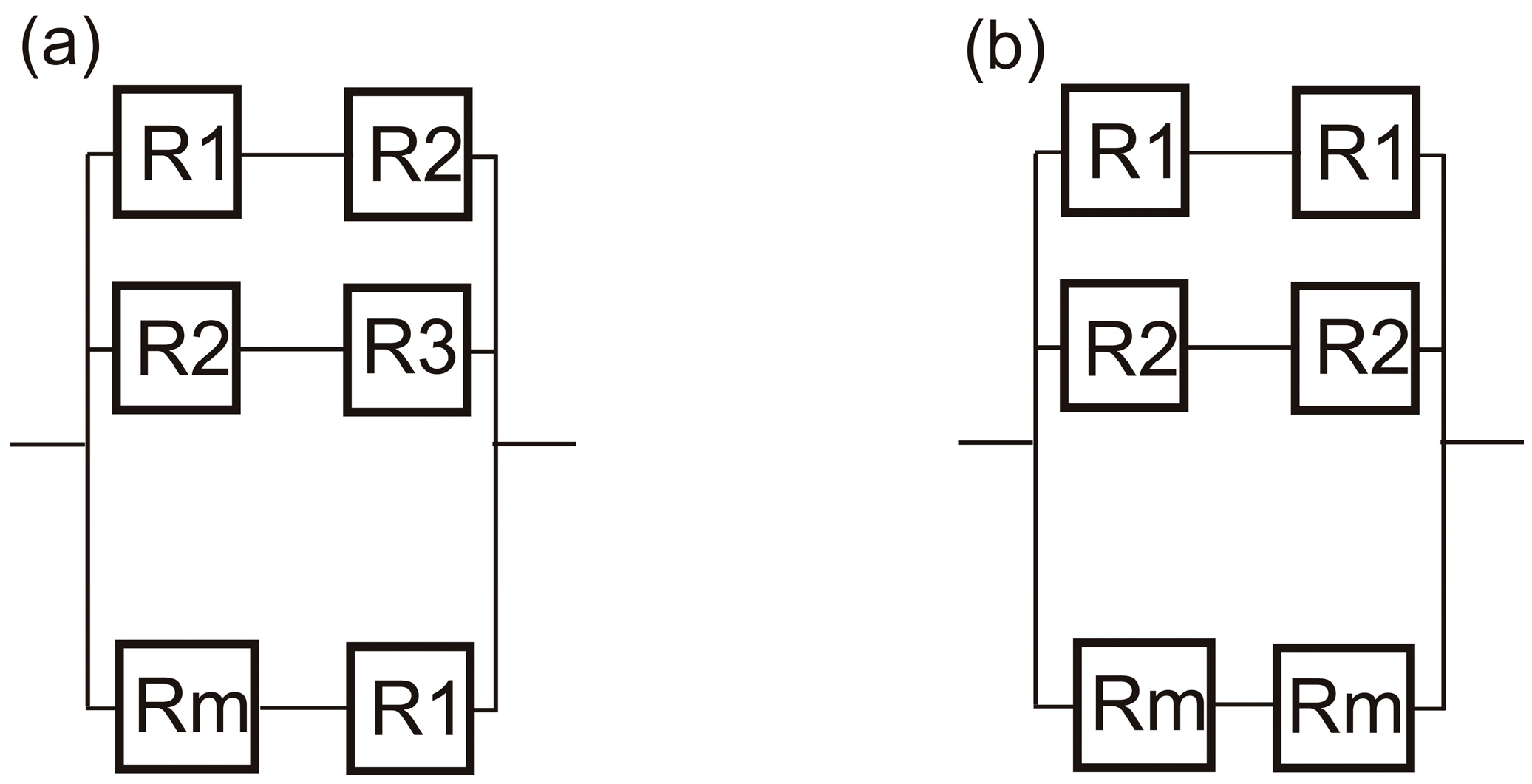
Figure 1. (a) The reliability network of a parallel system with interchangeable components of different varieties with (a) asymmetric and (b) symmetric arrangements of the interchangeable components.
Mathematics 13 01381 g001
Figure 2. A reliability network demonstrating that no ranking of the reliabilities of the component varieties is necessary to apply the reliability improvement method: (a) a system with an asymmetric arrangement of the interchangeable components; (b) a system with a symmetric arrangement of the interchangeable components.
Mathematics 13 01381 g002
Figure 3. (a) The initial parallel system; (b) the parallel system with improved reliability; (c) the parallel system with maximised reliability, obtained by destroying the asymmetry in all parts of the system (a); (d) a subsystem, connected in parallel within the system in (b); (e) a subsystem, connected in parallel within the system in (c).
Mathematics 13 01381 g003
Figure 4. A system of m = 3 pipelines transporting cooling fluid to a chemical reactor CR with two pumping stations on each branch: (a) an asymmetric arrangement of the pumping station types in the branches; (b) a symmetric arrangement of the pumping station types in the branches.
Mathematics 13 01381 g004
Figure 5. A system of interchangeable sensors of varieties X and Y, measuring the temperature/pressure/concentration in two zones, A and B: (a) an asymmetric arrangement of the sensors in the zones; (b) a symmetric arrangement of the sensors in the zones; (c) the reliability network of the system in (a); (d) the reliability network of the system in (b).
Mathematics 13 01381 g005
Figure 6. Functional diagrams of two different arrangements of the interchangeable pumping sections on three pipelines: (a) an asymmetric arrangement of the pumping sections; (b) a symmetric arrangement of the pumping sections.
Mathematics 13 01381 g006
Figure 7. Reliability networks of the systems in Figure 6: (a) the reliability network of the system in Figure 6a; (b) reliability network of the system in Figure 6b.
Mathematics 13 01381 g007
Figure 8. (a) A reliability network obtained from the physical interpretation of the right-hand side of Inequality (4) and (b) a reliability network obtained from the physical interpretation of the left-hand side of Inequality (4).
Mathematics 13 01381 g008
Figure 9. (a) A reliability network obtained from the physical interpretation of the right-hand side of Inequality (5) and (b) a reliability network obtained from the physical interpretation of the left-hand side of Inequality (5).
Mathematics 13 01381 g009
Figure 10. (a) A reliability network obtained from the physical interpretation of the right-hand side of Inequality (6) and (b) a reliability network obtained from the physical interpretation of the left-hand side of Inequality (6).
Mathematics 13 01381 g010
Figure 11. (a) A reliability network with interchangeable redundancies with (a) a symmetric and (b) an asymmetric arrangements of the interchangeable redundancies.
Mathematics 13 01381 g011
Figure 12. A system of n pipelines transporting toxic fluid with two valves of types A1, A2, …, Am, on each pipeline; (a) a symmetric arrangement of redundancies; (b) an asymmetric arrangement of redundancies.
Mathematics 13 01381 g012
Table 1. The reliabilities of the systems in Figure 2 for different values of the reliabilities of the component varieties forming the systems.
r1r2r3r4FaFb
0.610.920.750.450.0650.034
0.20.60.10.70.6620.31
0.80.40.650.220.3550.166
0.10.750.650.120.4320.246
0.850.550.880.460.09960.0344
0.50.70.250.70.2880.183
0.350.480.700.140.4740.338
0.10.20.150.70.7910.474
0.890.990.790.959.987 × 10−41.51 × 10⁻⁴
Table 2. The reliabilities of the systems in Figure 5 for different values of the reliabilities of the sensors.
r1r2FaFb
0.160.850.750.27
0.760.40.480.35
0.90.20.670.18
0.850.320.530.24
0.090.70.880.5
0.10.70.8650.505
0.980.946.21 × 10−34.61 × 10⁻³
Table 3. The reliabilities of the systems in Figure 12 for different values of the probabilities of failure of the components forming the systems.
f1f2f3f4RaRb
0.70.30.870.430.0920.255
0.320.560.450.680.2640.333
0.880.200.400.910.0310.131
0.210.350.120.540.5850.830
0.560.230.780.390.2160.389
0.750.420.450.880.06480.114
0.10.70.250.190.4560.716
0.980.890.820.914.63 × 10−49.48 × 10⁻⁴
Disclaimer/Publisher’s Note: The statements, opinions and data contained in all publications are solely those of the individual author(s) and contributor(s) and not of MDPI and/or the editor(s). MDPI and/or the editor(s) disclaim responsibility for any injury to people or property resulting from any ideas, methods, instructions or products referred to in the content.