Reinforcement Learning for Mitigating Malware Propagation in Wireless Radar Sensor Networks with Channel Modeling

Abstract

With the rapid development of research on Wireless Radar Sensor Networks (WRSNs), security issues have become a major challenge. Recent studies have highlighted numerous security threats in WRSNs. Given their widespread application value, the operational security of WRSNs needs to be ensured. This study focuses on the problem of malware propagation in WRSNs. In this study, the complex characteristics of WRSNs are considered to construct the epidemic VCISQ model. The model incorporates necessary factors such as node density, Rayleigh fading channels, and time delay, which were often overlooked in previous studies. This model achieves a breakthrough in accurately describing real-world scenarios of malware propagation in WRSNs. To control malware spread, a hybrid control strategy combining quarantine and patching measures are introduced. In addition, the optimal control method is used to minimize control costs. Considering the robustness and adaptability of the control method, two model-free reinforcement learning (RL) strategies are proposed: Proximal Policy Optimization (PPO) and Multi-Agent Proximal Policy Optimization (MAPPO). These strategies reformulate the original optimal control problem as a Markov decision process. To demonstrate the superiority of our approach, multi-dimensional ablation studies and numerical experiments are conducted. The results show that the hybrid control strategy outperforms single strategies in suppressing malware propagation and reducing costs. Furthermore, the experiments reveal the significant impact of time delays on the dynamics of the VCISQ model and control effectiveness. Finally, the PPO and MAPPO algorithms demonstrate superior performance in control costs and convergence compared to traditional RL algorithms. This highlights their effectiveness in addressing malware propagation in WRSNs.

1. Introduction

With their growing popularity, Wireless Radar Sensor Networks (WRSNs) have emerged as indispensable tools in diverse fields, ranging from environmental monitoring and target recognition to traffic tracking [1,2]. Harnessing radar technology, these networks provide advanced capabilities such as detection, safety monitoring, imaging, and outdoor tracking [3,4,5]. However, the widespread deployment and open nature of WRSNs have also rendered them vulnerable to malicious attacks [6,7,8,9]. Malware can swiftly propagate through these networks due to their complex propagation mechanisms, resulting in pervasive infection [10]. Consequently, a compromised device can inflict substantial damage, including data breaches, system disruptions, and privacy breaches [11]. Thus, combating the propagation of malware is paramount to safeguarding the security, reliability, and asset preservation of WRSNs.

In contrast to traditional Wireless Sensor Networks (WSNs) [6,7,10,12,13], the channel modeling of WRSNs has taken into account the interference issue between radar detection and communication [14]. However, current research on malware propagation in WRSNs is insufficient, with issues such as insufficient transmission power of radar sensors, variations in signal-to-noise ratio calculations during Rayleigh fading, the differences between realistic and ideal propagation, and the impact of radar node density and runtime on node contact rates. Given these unique problems, there is an urgent need to design more accurate epidemic models to explore the impact of radar channel communication on malicious propagation in WRSNs. Therefore, our primary goal is to develop a novel VCISQ malware propagation model that incorporates channel characteristics and radar density features. Meanwhile, to effectively contain the propagation of malware, further research is generally needed on optimal control issues. However, it is well known that the reported optimal control results are highly complex and dependent on the model still requiring much computation [6,12,13,15].

To address the highly complex issues involved in this model, the minimum cost problem is traditionally solved by the Hamilton–Jacobi–Bellman (HJB) equation. This approach is based on the assumption of full knowledge of the existing system [12,13,15]. However, its inherent nonlinearity and intractability render analytical methods difficult to employ for solving the HJB equation. Consequently, optimal control theory cannot be applied in all the practical applications. Compared to existing model-based optimal control strategies, it is necessary to find a suitable intelligent algorithm to implement a model-free control strategy. Recently, many end-to-end reinforcement learning (RL) methods provide model-free optimal control strategies [16,17], but few of them are related to optimal control problems in malware propagation of WRSN environments. Meanwhile, the growing popularity of Multi-Agent RL (MARL) in addressing optimal control issues in complex distributed systems provides a new direction [18]. MARL learns optimal strategies through interaction and collaboration within the environment.

Given the above motivations, in this study, model-free RL algorithms are adopted to tackle the control problem of WRSNs. The Proximal Policy Optimization (PPO) and Multi-Agent Proximal Policy Optimization (MAPPO) algorithms are applied for the first time in the field of controlling malware propagation in WRSNs. To our knowledge, this is the first study to establish a malware propagation model that simultaneously considers Rayleigh fading, node density, and delays. The feasibility of the optimal control theory results and the effectiveness of the algorithm control strategies are verified through numerical simulations. The main contributions of this study are as follows:

1.

A malware propagation model VCISQ is proposed, which incorporates Rayleigh fading, node density, and time delay to model malware propagation in WRSNs. Compared to other existing epidemic models, VCISQ accounts for additional critical factors influencing malware spread in WRSNs. This has to some extent improved the accuracy of depicting real scenes in WRSNs. To effectively combat malware propagation, hybrid patching and quarantine strategies are introduced. At the same time, the optimal control method under these strategies is derived. The optimal control outputs help preserve network integrity by protecting data transmission against malware interference, thereby enhancing the performance of WRSNs. Furthermore, the optimal control method provides a theoretical benchmark solution for static propagation models, offering a reference baseline for evaluating the performance of RL methods.

2.

To achieve more practical and adaptive control schemes that can boost the performance of WRSNs, two novel model-free RL algorithms, PPO and MAPPO, are introduced for the first time to suppress malware propagation in WRSNs. PPO employs a clipping parameter to limit policy updates, minimizing the risks associated with sub-optimal control decisions. This not only enhances the efficiency of malware suppression but also improves the adaptability of the network to dynamic changes in the environment. In WRSNs, such adaptability is crucial for maintaining high-performance operation as environmental factors can vary rapidly. On the other hand, MAPPO leverages a Centralized Training, Decentralized Execution (CTDE) framework. This framework allows for more efficient learning and decision-making across multiple agents in the WRSN. As a result, it can better coordinate the actions of different nodes in the network, leading to more effective suppression of malware and ultimately enhancing the overall performance of WRSNs.

3.

To validate the effectiveness of the proposed model and its associated control strategies in improving WRSN performance, this study compares the performance differences between the optimal control and RL algorithms under various scenarios. The experimental results indicate that both PPO and MAPPO algorithms demonstrate excellent adaptability when facing changes in environmental parameters. In WRSNs, environmental parameter changes can cause significant performance fluctuations. The ability of PPO and MAPPO to adapt well means that they can maintain stable and high-performance operation. Compared to traditional control strategies such as Deep Q-Network (DQN) [19] and Double Deep Q-Network (DDQN) [20], PPO and MAPPO are able to more precisely regulate information propagation. This precise regulation ensures that data are transmitted in an optimal manner, reducing the negative impact of malicious programs on network performance. As a result, WRSNs equipped with these algorithms can operate more efficiently and with higher reliability, thus significantly enhancing the overall performance of WRSNs.

The remaining parts of this study are organized as follows: Section 2 introduces the preliminary work. In Section 3, a novel VCISQ model and the corresponding hybrid optimal control scheme are proposed. Section 4 presents the two model-free RL algorithms. Section 5 covers the numerical analysis and simulation results. Section 6 discusses some future directions.

2. Related Work

(1) Modeling Methods of Epidemic Theory: Currently, modeling methods based on epidemiological models have been adopted by scholars in many fields to study the dynamic evolution process of malware propagation [12,13,15,21,22], worm propagation [23], cyber physical systems [24], Industrial Internet of Things (IIoT) [25], and rumor propagation [26,27]. The SCIRS epidemic model was proposed to describe the propagation of malware [21], and it is worth noting that their work considered the population dynamics of WSNs, vaccination, and re-infection processes. A stochastic epidemic model that considers the stochastic disturbance of the cross-infection of malware in UAV-WSN was proposed [22]. A malware propagation model was proposed that takes into account the influence of sleeping state nodes on modeling [13]. An SEIR model with two time delays was proposed to study the dynamic propagation of worms in WSNs [23], considering the exposure period and immunity period during worm outbreaks. However, to our knowledge, more accurate characteristics of WRSNs, such as insufficient transmission power of radar sensors, changes in Rayleigh fading calculation due to the signal-to-noise ratio, differences between realistic propagation and ideal propagation, and the impact of radar node density and operation time on node contact rate, are rarely considered in existing models of WRSN malware propagation. Therefore, a time-delayed WRSN malware propagation model incorporating channel propagation characteristics is proposed to address the above shortcomings.

(2) Prevention and Propagation Control of Network Attacks: Detecting and preventing cyberattacks is the first step to ensuring security and stability. Many researchers have delved into this area [28,29,30,31]. In [28], a behavior sequence was constructed and combined with a transformer-based multi-sequence fusion classifier to achieve efficient detection of encrypted malware traffic. In [29], five different attention mechanism modules were integrated into the ResNeXt network for malware detection and classification. In [30], a deep neural network-based malware detection method was proposed, which effectively improved the accuracy of malware detection. In [31], an RL-based generation framework called RLAEG was proposed to enhance the detection capability of an Intrusion Detection System (IDS) to static malware. In addition, various control measures have been investigated by scholars to enable timely mitigation of the propagation of cyberattacks [32,33,34]. For example, patching was used to control the formation of botnets [32]. In the study [33], a combined control strategy of vaccination and isolation was implemented to maintain the stability of worm attacks in mobile networks. A hybrid optimal control strategy, which includes continuous isolation propagation and pulse rumor isolation with time delay, was adopted and proved to have excellent control effects [34]. However, most research has primarily focused on the detection and prevention of network attacks. By contrast, relatively limited attention has been devoted to understanding the propagation mechanisms of network attacks. Therefore, a hybrid time delay optimal control strategy combining isolation-control and patching-control has been adopted in this study to control the propagation of malware in WRSNs.

(3) Traditional Control Methods: Recent scholarly investigations have evaluated various mathematically modeled control strategies for combating malware propagation [24,25,35,36]. In [24], Conventional PD feedback control was leveraged in to combat malware propagation in cyber–physical systems. A differential game-theoretic framework was developed to counteract malware spread in IIoT environments [25]. In [35], researchers implemented fractional-order optimal control methods to suppress malware dissemination within the Internet of Vehicles (IoV). In [36], a sliding-mode control theory-based rapid response mechanism is proposed for effectively mitigating malware transmission in unmanned aerial vehicle systems. While these traditional approaches have demonstrated significance in malware containment, their effectiveness in WRSNs faces critical challenges due to dynamic channel instability and time-varying network topology [37,38]. The constant parameter model cannot accurately describe its propagation mechanism [36], but these methods all rely on precise mathematical models. For the optimal control method, it expects to iteratively predict the control strategy for the next moment through the set initial state [39]. As the model parameters continue to change during iterations, such open-loop control will gradually deviate from the global optimal strategy [40]. This will result in a decrease in the adaptability of the controller.

(4) The Methods of Model-Free Reinforcement Learning: Due to the rapid development and excellent performance of artificial intelligence, multiple learning algorithms have been used to solve such decision problems [16,17,18,41,42,43,44,45,46,47,48]. In [43], a deep RL algorithm was adopted to solve the resource allocation problem in radar communication. A deep RL algorithm was employed to address radar detection and tracking problems [44]. RL algorithms have been used to solve the optimal deployment problem in WSNs [45]. Machine learning has been applied to resolve the spread of malware in the Internet of Underwater Things (IoUT) [41]. The PPO algorithm was employed to solve the Markov decision optimization problem of intercepting maneuvering targets [46]. In such complex problems, model-free RL algorithms have demonstrated excellent learning performance by optimizing decision strategies through interaction with the environment. This aligns more closely with the uncertainties and complexities encountered in practical applications.

(5) The Superiority of PPO and MAPPO methods: Good performance has been demonstrated by the PPO algorithm in model-free RL on many tasks [17,47]. On the AVG path planning method decision [17], the outstanding control effect of PPO was validated. The PPO algorithm was adopted to accomplish the dynamic mapping and scheduling decisions of service chains. Due to its use of clipped values [47], the PPO algorithm can constrain the range of extreme updates in policy training, thereby improving sample efficiency and algorithm stability. Additionally, it exhibits better empirical sample complexity than Trust Region Policy Optimization (TRPO). Therefore, for more practicality and feasibility, the model-free PPO algorithm is considered to minimize system costs of patching and isolation, thereby breaking free from the constraints of model-based optimal control. Furthermore, MARL has also been applied to such problems. It learns to achieve a given global objective by dynamically interacting with a common environment through multiple agents. As a multi-agent algorithm of PPO, MAPPO can find excellent control strategies in decision-making problems of this kind. For example, MAPPO was utilized to solve resource allocation problems for collaborative drones [48], while MARL was used to achieve strategic performance in multi-agent resource allocation [49]. Compared to MADDPG and QMIX algorithms, MAPPO can achieve good control effects [50]. The framework of employing clipped values along with centralized training and distributed execution was also adopted. In this framework, the overall information of all agents is used during training to ensure that each agent can independently infer the optimal strategy based on its local information. However, there is currently no research on the use of PPO and MAPPO algorithms for optimal control in practical malware propagation in WRSNs. Therefore, to fully exploit the potential of RL algorithms in WRSNs, this study presents the first attempt to introduce PPO and MAPPO for combating the propagation of malware.

The comparison of the attributes between this study and various reference documents is presented in

Table 1. The comparison of attributes between this study and various reference documents.

Study	Main Research	Characteristics of Model Construction			Control Method		Optimal Control	RL Algorithms
		Epidemic	Channel	Time Delay	Quarantine	Patching
Shen et al. [13]	Optimized control	✔	✘	✘	✘	✘	✔	✘
Sun et al. [16]	Optimized control	✘	✘	✘	✘	✘	✔	✘
Kuai et al. [17]	Optimized control	✘	✘	✘	✘	✘	✘	✔ (PPO)
Xiao et al. [18]	Optimized control	✘	✘	✘	✘	✘	✘	✔
Zhuang et al. [24]	Optimized control	✔	✘	✔	✘	✔	✘	✘
Farooq and Zhu [32]	Optimized control	✘	✘	✘	✔	✘	✔	✘
Lee et al. [43]	Optimized control	✘	✘	✘	✘	✘	✘	✔
Thornton et al. [44]	Optimized control	✘	✘	✘	✘	✘	✘	✔
Guo and Jafarkhani [45]	Optimized control	✘	✘	✘	✘	✘	✘	✘
Guo et al. [46]	Optimized control	✘	✘	✘	✘	✘	✘	✔ (PPO)
Wang et al. [47]	Optimized control	✘	✘	✘	✘	✘	✘	✔ (PPO)
Kang et al. [48]	Optimized control	✘	✘	✘	✘	✘	✘	✔ (MAPPO)
Yu et al. [49]	Optimized control	✘	✘	✘	✘	✘	✘	✔ (MARL)
Cui et al. [50]	Optimized control	✘	✘	✘	✘	✘	✘	✔ (MAPPO)
Jafar et al. [51]	Optimized control	✔	✘	✘	✘	✘	✔	✔
Proposed framework	Optimized control	✔	✔	✔	✔	✔	✔	✔ (PPO/MAPPO)

.

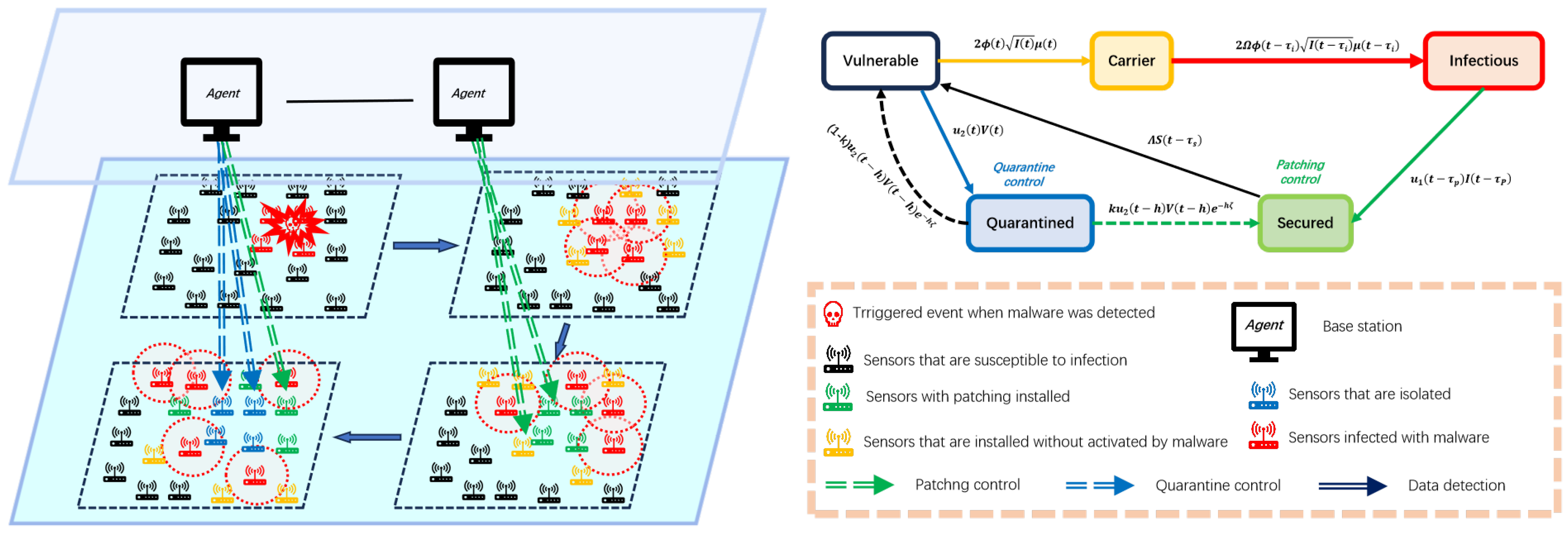
3. Model Establishment and Optimal Control Problem

In order to control the propagation of malware, we artificially install patches on the affected nodes and isolate the susceptible nodes. The controlled WRSN epidemic model introduces the recovered nodes (S-nodes) to describe the nodes that have installed patches and no longer propagate the malware. The isolated nodes (Q-nodes) are introduced to describe the nodes that have been isolated and are not affected by the malware. The rate from the state I-nodes to S-nodes is determined as a continuous control $u_1\left(t\right)$. The rate from the state V-nodes to Q-nodes is also defined as a continuous control $u_2\left(t\right)$.

As illustrated in Figure 1, five compartments are introduced to describe different states of nodes and its propagation process is demonstrated. Sensors with vulnerabilities become V-nodes, and once attacked, these nodes may enter a dormant state. These nodes are referred to as C-nodes. Taking into account the temporal nature of malware infection, after a certain time ${\tau }_i$, the malware becomes activated. Nodes carrying the malware will be infected and propagate the malware to attack other nodes. Such nodes are referred to as I-nodes. Over time, some infected I-nodes are repaired through manual intervention, becoming S-nodes that are no longer susceptible to the infection. After a period of time ${\tau }_p$, the effectiveness of the patching program decreases for S-nodes, causing them to revert back to V-nodes. In addition to this, V-nodes can be quarantined and protected manually, transforming into Q-nodes. After some time, certain Q-nodes are no longer protected and revert back to vulnerable V-nodes, while some Q-nodes are patched and become S-nodes. The remaining nodes are kept quarantined for continued protection.

To reveal the cross-propagation of malware in WRSNs, we calculate the malware carrying rate from V-nodes to C-nodes and the infection rate from C-nodes to I-nodes based on the dynamic nature of information propagation. The relevant parameters are explained in

Table 2. Relevant parameters.

Parameters	Description
N	Number of wireless radar sensors
$\varphi \left(t\right)$	The number of neighbors of a I-node that can be infected
$\mu \left(t\right)$	Real-time contact rate
a	Slide length of the target square area
$\lambda$	The density of total nodes
q	The communication difference coefficient between ideal and reality
${\gamma }_{th}$	Signal-to-noise threshold
$\rho$	Density of total nodes
$\eta$	The number of nodes around any node that can receive information
$\chi$	Transmit power coefficient
$\Omega$	Malware installation success rate
${\tau }_i$	Malware installation delay
${\tau }_p$	Patch installation delay
${\tau }_s$	Patch failure delay
$\mathit{\Lambda }$	Patch failure rate
$\kappa$	Quarantine rate
${\sigma }_n^2$	Background noise power
$\zeta$	Quarantine retention exponent
$\alpha$	Path loss exponent
h	Quarantine failure delay
t	Working cycle
T	Maximum number of episodes

.

The interaction range of the radar nodes is modeled as a square area with side length a. Considering the characteristics of WRSNs, Rayleigh fading is taken into account between any two radars. The small-scale fading is represented by v, which follows a distribution $\mathcal{C}\mathcal{N}\left(0,1\right)$, and the large-scale path loss is represented by p. Consequently, the channel coefficient g can be expressed as $g=v\sqrt{p}$.

3.1. The Number of Susceptible Neighboring Nodes $\varphi \left(t\right)$ with Rayleigh Fading

It is assumed that the total infected I-nodes are only within a circle containing infected nodes. As a result, susceptible V-nodes can only interact with infected I-nodes around the circumference of the circle. Based on the data propagation dynamics [41], the infection rate (from V-nodes to C-nodes) of susceptible nodes carrying malware is represented as $2\varphi \left(t\right)\sqrt{I\left(t\right)}\mu \left(t\right)$, where $\varphi \left(t\right)$ represents the number of susceptible neighboring nodes and $\mu \left(t\right)$ represents the contact rate between V-nodes and I-nodes.

The observed signal-to-noise ratio (SNR) of a node must be higher than the SNR threshold ${\gamma }_{th}$ in order to successfully receive the node’s information. Considering the small-scale fading v, the distance between communication nodes $r_d$, the background noise power ${\sigma }_n$, the transmit power $p_t$, the channel coefficient g, and the transmit power coefficient $\chi$, the observed SNR at a radar node can be expressed as ${\Phi }_c=p_t{\left|g\right|}^2/{\sigma }_n^2=p_t{P}_0{\left|v\right|}^2/\left({\sigma }_n^2{r}_d^{\alpha }\right)=\chi {\left|v\right|}^2/\left({\sigma }_n^2{r}_d^{\alpha }\right)$. The reception success rate is given as $P_{in}=P_r\left({\Phi }_c⩾{\gamma }_{th}\right)$. Additionally, within the range of the randomly infected nodes in the target area, the neighboring nodes are approximately uniformly distributed, while the Rayleigh fading is taken into account in the channel communication. Consequently, the number of the neighboring nodes that receive information from any node can be calculated as

$$\begin{array}{cc}\hfill \eta =& {\displaystyle \frac{2\rho \pi {\chi }^{\frac{2}{a}}}{\alpha {\sigma }_n^{\frac{4}{a}}{\gamma }_{th}^{\frac{2}{a}}}}\mathit{\Gamma }\left({\displaystyle \frac{2}{a}}\right)·P.\hfill \end{array}$$

(1)

where $\mathit{\Gamma }\left(t\right)={\int }_0^{\infty }{t}^{x-1}{e}^{-t}dt$ is the gamma function, and a is the path loss exponent. Finally, considering the difference between the ideal and real communication q, the number of the susceptible neighboring nodes $\varphi \left(t\right)$ can be represented as

$$\begin{array}{cc}\hfill \varphi \left(t\right)=& \sqrt{{\displaystyle \frac{2q\pi {\chi }^{\frac{2}{a}}}{\alpha {\sigma }_n^{\frac{4}{a}}{\gamma }_{th}^{\frac{2}{a}}{a}^2}}\mathit{\Gamma }\left({\displaystyle \frac{2}{a}}\right)V\left(t\right)}.\hfill \end{array}$$

(2)

3.2. Contact Rate Between Neighboring Nodes

In dynamic processes with relatively low node density, the contact rate between susceptible and infected nodes is decreased, as the susceptible nodes may not come into contact with the infected nodes. The contact rate is represented as $k\approx 1-e^{-{\displaystyle \frac{1}{2}}\eta }$, considering the significant impact of node density. Additionally, the insufficient transmission power of the devices is taken into account. As time progresses, the transmission power of the nodes decreases, leading to insufficient power during message propagation and gradually causing interruptions in the message transmission. Consequently, the node contact rate is expressed as an exponential function of time, denoted as $\mu \left(t\right)={\left(1-e^{-{\displaystyle \frac{1}{2}}\eta }\right)}^t$ [14].

3.3. Malware Propagation Model

Considering the aforementioned analysis, the hybrid control model can be described as

$$\begin{array}{cc}\hfill \overline{V}\left(t\right)={\displaystyle \frac{dV}{dt}}=& -2\varphi \left(t\right)\sqrt{I\left(t\right)}\mu \left(t\right)+\mathit{\Lambda }S\left(t-{\tau }_s\right)-u_2\left(t\right)\hfill \\ \hfill & V\left(t\right)+\left(1-k\right)u_2\left(t-h\right)V\left(t-h\right)·e^{-h\zeta },\left(Remark1\right)\hfill \\ \hfill \overline{C}\left(t\right)={\displaystyle \frac{dC}{dt}}=& 2\varphi \left(t\right)\sqrt{I\left(t\right)}\mu \left(t\right)\hfill \\ \hfill & -2\Omega \varphi \left(t-{\tau }_i\right)\sqrt{I\left(t-{\tau }_i\right)}\mu \left(t-{\tau }_i\right),\hfill \\ \hfill \overline{I}\left(t\right)={\displaystyle \frac{dI}{dt}}=& 2\Omega \varphi \left(t-{\tau }_i\right)\sqrt{I\left(t-{\tau }_i\right)}\mu \left(t-{\tau }_i\right)\hfill \\ \hfill & -u_1\left(t-{\tau }_p\right)I\left(t-{\tau }_p\right),\hfill \\ \hfill \overline{S}\left(t\right)={\displaystyle \frac{dS}{dt}}=& u_1\left(t-{\tau }_p\right)I\left(t-{\tau }_p\right)-\mathit{\Lambda }S\left(t-{\tau }_s\right)\hfill \\ \hfill & +k{u}_2\left(t-h\right)V\left(t-h\right)·e^{-h\zeta },\hfill \\ \hfill \overline{Q}\left(t\right)={\displaystyle \frac{dQ}{dt}}=& u_2\left(t\right)V\left(t\right)-k{u}_2\left(t-h\right)V\left(t-h\right)·e^{-h\zeta }\hfill \\ \hfill & -\left(1-k\right)u_2\left(t-h\right)V\left(t-h\right)·e^{-h\zeta }.\hfill \end{array}$$

(3)

where $\overline{V}\left(t\right),\overline{C}\left(t\right),\overline{I}\left(t\right),\overline{S}\left(t\right),\overline{Q}\left(t\right)\ge 0,\overline{V}\left(t\right)+\overline{C}\left(t\right)+\overline{I}\left(t\right)+\overline{S}\left(t\right)+\overline{Q}\left(t\right)=N$.

Remark 1.

Unlike the conventional isolation measure models of other wireless radar sensors [33,34], the isolation time-lag and attenuation are taken into account in this study. In the kinetic Equation (3), $e^{-h\zeta }$ represents the isolation decay parameter, whose value is jointly determined by parameters h and ζ. From the perspective of real-world scenarios, isolation measures are not absolutely effective. Taking h as the isolation time-lag coefficient as an example, when the value of h increases, the value of $e^{-h\zeta }$ decreases accordingly. This indicates that the degree of attenuation of the isolation effect intensifies. Incorporating $e^{-h\zeta }$ into the equation system of the malware propagation model can more accurately depict the internal relationship between the dynamic evolution process of the node states within the system and the isolation measures. Thus, it provides a solid theoretical basis for designing highly efficient and practical malware propagation control strategies.

The problem of hybrid system control involves two control strategies: installation of patching programs and quarantine. The objective is to minimize the number of susceptible nodes, infected nodes, isolated nodes, and the overall cost associated with the two control strategies. By employing the Pontryagin’s minimum principle, we will derive the necessary conditions for optimal control and obtain the solution for hybrid optimal control.

3.4. Optimal Control Problem

This section is designed to solve the problem of computational optimization of control. The relevant parameter symbols are described in

Table 3. The values of relevant parameters.

	Parameters	Values
WRSNs	Number of wireless radar sensors N	300
	Slide length of the target square area a	500 m
	The density of total nodes $\lambda$	$1.2\times {10}^{-3}$
	The communication difference coefficient between ideal and reality q	$2\mathrm{l}\mathrm{n}2/\pi$
	Signal-to-noise threshold ${\gamma }_{th}$	3 dB
	Transmit power coefficient $\chi$	$5\times {10}^{-10}$
	Malware installation success rate $\Omega$	0.8
	Malware installation delay ${\tau }_i$	1
	Patch installation delay ${\tau }_p$	0.5
	Patch failure delay ${\tau }_s$	2
	Patch failure rate $\mathit{\Lambda }$	0.05
	Quarantine rate $\kappa$	0.5
	Background noise power ${\sigma }_n^2$	−60 dBm
	Quarantine retention exponent $\zeta$	0.05
	Path loss exponent $\alpha$	4
	Quarantine failure delay h	1
	The weighted cost parameter for V-nodes $A_v$	300
	The weighted cost parameter for I-nodes $A_i$	900
	The weighted cost parameter for Q-nodes $A_q$	300
	The weighted cost of patching-control $A_{u_1}$	12
	The weighted cost of quarantine-control $A_{u_2}$	12
PPO	AC network learning rate	$2\times {10}^{-4}$
	Clipping parameter	0.2
	Experience buffer sizes	1024
	Batch size	64
	Value discount factor $\gamma$	0.99
	Entropy coefficient of the policy $\sigma$	0.01
MAPPO	AC network learning rate	$2\times {10}^{-4}$
	Clipping parameter	0.2
	Experience buffer sizes	200
	Batch size	200
	Value discount factor $\gamma$	0.99
	Entropy coefficient of the policy $\sigma$	0.01
DQN	Learning rate	$2\times {10}^{-4}$
	Update frequency	4
	Experience buffer sizes	1024
	Batch size	64
	Value discount factor $\gamma$	0.99
DDQN	Learning rate	$2\times {10}^{-4}$
	Update frequency	4
	Experience buffer sizes	1024
	Batch size	64
	Value discount factor $\gamma$	0.99

. Set the system running time to $t\in \left[0,T\right]$. Based on the system (3), the cost function is described as follows:

$$\begin{array}{cc}\hfill U=& {\int }_0^T[A_{v}V\left(t\right)+{\left(A_{i}I\left(t\right)\right)}^{\beta }+A_{q}Q\left(t\right)+A_{u_1}{u_1}^2\left(t\right)+A_{u_2}{u_2}^2\left(t\right)]dt.\left(Remark2\right)\hfill \end{array}$$

(4)

where $\beta$ is the attack severity of the malware. $A_v$ is the weighted cost parameters for V-nodes. $A_i$ is the weighted cost parameters for I-nodes. $A_q$ is the weighted cost parameter for Q-nodes. $A_{u_1}$ is the weighted cost parameter associated with the use of patching-control. $A_{u_2}$ is the weighted cost parameter associated with the use of quarantine-control.

Remark 2.

The design of the cost function (4) is highly innovative, as the parameter β is introduced to characterize the severity of malware attacks. In the traditional cost function of reference [15,51], the weights of various costs are fixed uniformly. In contrast, this design can more flexibly and accurately reflect the cost variations in different attack scenarios. By adjusting the value of β, the weight of the impact of the number of infected nodes on the total cost can be dynamically adjusted according to the actual situation. This enables the control strategy to optimize costs more rationally when facing malware attacks of different severity levels, thus enhancing the practicality and adaptability of the model.

The continuous Hamiltonian function is introduced as follows:

$$\begin{array}{cc}\hfill H\left(t\right)& =A_{v}V\left(t\right)+{\left(A_{i}I\left(t\right)\right)}^{\beta }+A_{q}Q\left(t\right)+A_{u_1}{u_1}^2\left(t\right)+A_{u_2}{u_2}^2\left(t\right)+{\lambda }_1\left(t\right)[-2\varphi \left(t\right)\sqrt{I\left(t\right)}\mu \left(t\right)\hfill \\ \hfill & +\mathit{\Lambda }S\left(t-{\tau }_i\right)-u_2\left(t\right)V\left(t\right)+\left(1-k\right)u_2\left(t-h\right)V\left(t-h\right)·e^{-h\zeta }]+{\lambda }_2\left(t\right)[2\varphi \left(t\right)\sqrt{I\left(t\right)}\mu \left(t\right)\hfill \\ \hfill & -2\Omega \varphi \left(t-{\tau }_i\right)\sqrt{I\left(t-{\tau }_i\right)}\mu \left(t-{\tau }_i\right)]+{\lambda }_3\left(t\right)[2\Omega \varphi \left(t-{\tau }_i\right)\sqrt{I\left(t-{\tau }_i\right)}\mu \left(t-{\tau }_i\right)-u_1\hfill \\ \hfill & \left(t-{\tau }_p\right)I\left(t-{\tau }_p\right)]+{\lambda }_4\left(t\right)[u_1\left(t-{\tau }_p\right)I\left(t-{\tau }_p\right)-\mathit{\Lambda }S\left(t-{\tau }_s\right)+k{u}_2\left(t-h\right)V(t-h)\hfill \\ \hfill & e^{-h\zeta }]+{\lambda }_5\left(t\right)[u_2\left(t\right)V\left(t\right)-k{u}_2\left(t-h\right)V\left(t-h\right)·e^{-h\zeta }-\left(1-k\right)u_2\left(t-h\right)V\left(t-h\right)·e^{-h\zeta }].\hfill \end{array}$$

(5)

Theorem 1.

If $\delta U=0$, the necessary conditions of optimality for the system (3) can be obtained as follows:

(1)

The adjoint equations are described as

$$\begin{array}{c}\hfill \dot{\lambda }\left(t\right)=-[{\displaystyle \frac{\partial H\left(t\right)}{\partial x\left(t\right)}}+\phi \left[0^{+},T-\tau \right]{\displaystyle \frac{\partial H\left(t+\tau \right)}{\partial x\left(t\right)}}].\end{array}$$

(6)

where $x\left(t\right)$ is state nodes of the system (3), and ${\phi }_t\left[a,b\right]=1$ is a characteristic function. More precisely, ${\phi }_t\left[a,b\right]=1$ if $t\in \left[a,b\right]$ and zero otherwise.

(2)

The boundary condition is given by

$$\begin{array}{c}\hfill \lambda \left(t_f\right)={\displaystyle \frac{\partial \varphi \left(x\left(t_f\right)\right)}{\partial x\left(t_f\right)}}=0.\end{array}$$

(7)

where ${\phi }_t\left[a,b\right]=1$ is a characteristic function.

(3)

The optimal control $u^{opt}\left(t\right)$ satisfies

$$\begin{array}{c}\hfill {\displaystyle \frac{\partial H\left(t\right)}{\partial u\left(t\right)}}=0.\end{array}$$

(8)

Proof. 

Consider the following optimal hybrid control system, it has continuous state variables related to time delay. The time delay of continuous state variables is $\tau$.

$$\begin{array}{c}\hfill \dot{x}\left(t\right)=f\left(x\left(t\right),u\left(t\right),x\left(t-\tau \right)\right).\end{array}$$

(9)

where $u\left(t\right)$ are the continuous control variables. Then, the objective function is given as

$$\begin{array}{c}\hfill U=E\left\{\varphi \left[x\left(t_f\right)\right]\right\}+{\int }_0^T\left[H\left(t\right)-\lambda \left(t\right)\dot{x}\left(t\right)\right]dt.\end{array}$$

(10)

The first-order differential of Equation (10) is calculated as follows:

$$\begin{array}{cc}\hfill \delta U& =\left({\displaystyle \frac{\partial \varphi \left(x\left(t_f\right)\right)}{\partial x\left(t_f\right)}}-\lambda \left(t_f\right)\right)\delta x\left(t_f\right)+{\int }_0^T\left[\left({\displaystyle \frac{\partial H\left(t\right)}{\partial x\left(t\right)}}+\phi \left[0^{+},T-\tau \right]{\displaystyle \frac{\partial H(t+\tau )}{\partial x\left(t\right)}}+\dot{\lambda }\left(t\right)\right)\right.\hfill \\ \hfill & \left.\delta x\left(t\right)+{\displaystyle \frac{\partial H\left(t\right)}{\partial u\left(t\right)}}\delta u\left(t\right)+\left({\displaystyle \frac{\partial H\left(t\right)}{\partial u\left(t\right)}}-\dot{x}\left(t\right)\right)\delta \lambda \left(t\right)\right]dt.\hfill \end{array}$$

(11)

When $\delta U$= 0, the necessary conditions of optimality can be obtained as follows:

$$\begin{array}{cc}\hfill & \dot{\lambda }\left(t\right)=-\left[{\displaystyle \frac{\partial H\left(t\right)}{\partial x\left(t\right)}}+\phi \left[0^{+},T-\tau \right]{\displaystyle \frac{\partial H\left(t+\tau \right)}{\partial x\left(t\right)}}\right].\hfill \\ \hfill & \lambda \left(t_f\right)={\displaystyle \frac{\partial \varphi \left(x\left(t_f\right)\right)}{\partial x\left(t_f\right)}}=0.\hfill \\ \hfill & {\displaystyle \frac{\partial H\left(t\right)}{\partial u\left(t\right)}}=0.\hfill \end{array}$$

(12)

Thus, Theorem 1 has been proven.    □

Theorem 2.

The hybrid optimal control (patching-control and quarantine-control) solution of the system (3) is given as follows:

$$\begin{array}{cc}\hfill {\dot{\lambda }}_1\left(t\right)& =-\left[{\displaystyle \frac{\partial H\left(t\right)}{\partial V\left(t\right)}}+{\phi }_t\left[0^{+},T-{\tau }_i\right]{\displaystyle \frac{\partial H(t+{\tau }_i)}{\partial V\left(t\right)}}\right.\left.+{\phi }_t\left[0^{+},T-h\right]{\displaystyle \frac{\partial H(t+h)}{\partial V\left(t\right)}}\right]\hfill \\ \hfill & =-\left[A_v+\left({\lambda }_2\left(t\right)-{\lambda }_1\left(t\right)\right){\displaystyle \frac{\varphi \left(t\right)}{V\left(t\right)}}\sqrt{I\left(t\right)}\mu \left(t\right)\right.+\left({\lambda }_5\left(t\right)-{\lambda }_1\left(t\right)\right)u_2\left(t\right)\hfill \\ \hfill & -{\phi }_t\left[0^{+},T-{\tau }_i\right]{\lambda }_2(t+{\tau }_i)\Omega {\displaystyle \frac{\varphi \left(t\right)}{V\left(t\right)}}\sqrt{I\left(t\right)}\mu \left(t\right)+{\phi }_t\left[0^{+},T-{\tau }_i\right]{\lambda }_3(t+{\tau }_i)\Omega {\displaystyle \frac{\varphi \left(t\right)}{V\left(t\right)}}\sqrt{I\left(t\right)}\mu \left(t\right)\hfill \\ \hfill & +{\phi }_t\left[0^{+},T-h\right]{\lambda }_1(t+h)(1-k)u_2\left(t\right)e^{-h\zeta }+{\phi }_t\left[0^{+},T-h\right]{\lambda }_4(t+h)k{u}_2\left(t\right)e^{-h\zeta }\hfill \\ \hfill & \left.-{\phi }_t\left[0^{+},T-h\right]{\lambda }_5(t+h)u_2\left(t\right)e^{-h\zeta }\right],\hfill \end{array}$$

$$\begin{array}{cc}\hfill {\dot{\lambda }}_2\left(t\right)& =-{\displaystyle \frac{\partial H\left(t\right)}{\partial C\left(t\right)}}=0,\hfill \\ \hfill {\dot{\lambda }}_3\left(t\right)& =-\left[{\displaystyle \frac{\partial H\left(t\right)}{\partial I\left(t\right)}}+{\phi }_t\left[0^{+},T-{\tau }_p\right]{\displaystyle \frac{\partial H(t+{\tau }_p)}{\partial I\left(t\right)}}\right.\left.+{\phi }_t\left[0^{+},T-{\tau }_i\right]{\displaystyle \frac{\partial H(t+{\tau }_i)}{\partial I\left(t\right)}}\right]\hfill \\ \hfill & =-\left[\beta A_i{\left[A_{i}I\left(t\right)\right]}^{\beta -1}+\left({\lambda }_2\left(t\right)-{\lambda }_1\left(t\right)\right){\displaystyle \frac{\varphi \left(t\right)}{\sqrt{I\left(t\right)}}}\mu \left(t\right)\right.+{\phi }_t\left[0^{+},T-{\tau }_p\right]{\lambda }_4(t+{\tau }_p)u_1\left(t\right)\hfill \\ \hfill & -{\phi }_t\left[0^{+},T-{\tau }_p\right]{\lambda }_3(t+{\tau }_p)u_1\left(t\right)+{\phi }_t\left[0^{+},T-{\tau }_i\right]{\lambda }_3(t+{\tau }_i)\Omega {\displaystyle \frac{\varphi \left(t\right)}{\sqrt{I\left(t\right)}}}\mu \left(t\right)\hfill \\ \hfill & \left.-{\phi }_t\left[0^{+},T-{\tau }_i\right]{\lambda }_2(t+{\tau }_i)\Omega {\displaystyle \frac{\varphi \left(t\right)}{\sqrt{I\left(t\right)}}}\mu \left(t\right)\right],\hfill \\ \hfill {\dot{\lambda }}_4\left(t\right)& =-\left[{\displaystyle \frac{\partial H\left(t\right)}{\partial S\left(t\right)}}+{\phi }_t\left[0^{+},T-{\tau }_s\right]{\displaystyle \frac{\partial H(t+{\tau }_s)}{\partial S\left(t\right)}}\right]=-\left[{\phi }_t\left[0^{+},T-{\tau }_s\right]\left({\lambda }_1(t+{\tau }_s)-{\lambda }_4(t+{\tau }_s)\right)\mathit{\Lambda }\right],\hfill \\ \hfill {\dot{\lambda }}_5\left(t\right)& =-{\displaystyle \frac{\partial H\left(t\right)}{\partial Q\left(t\right)}}=-A_q.\hfill \end{array}$$

(13)

Its continuous adjoint equations satisfy Equation (13) with the transversality condition ${\lambda }_i\left(t_f\right)=0,i=1,\dots ,5$.

The optimization controls $u_1\left(t\right)$ and $u_2\left(t\right)$ are given by

$$\begin{array}{cc}\hfill 2A_{u_1}{u}_1^{opt}\left(t\right)& ={\phi }_t\left[0^{+},T-{\tau }_p\right]({\lambda }_3(t+{\tau }_p)-{\lambda }_4(t+{\tau }_p))I\left(t\right),\hfill \\ \hfill 2A_{u_2}{u}_2^{opt}\left(t\right)& =\left({\lambda }_1\left(t\right)-{\lambda }_5\left(t\right)\right)V\left(t\right)-{\phi }_t\left[0^{+},T-h\right]\left({\lambda }_1(t+h)-{\lambda }_5(t+h)\right)V\left(t\right)e^{-h\zeta }\hfill \\ \hfill & -{\phi }_t\left[0^{+},T-h\right]({\lambda }_4(t+h)-{\lambda }_1(t+h))kV\left(t\right)e^{-h\zeta }.\hfill \end{array}$$

(14)

Proof. 

According to the necessary conditions Equations (7) and (8) in Theorem 1, the objective function Equation (4) and the Hamiltonian function Equation (5), the continuous and impulsive adjoint equations are calculated as

$$\begin{array}{cc}\hfill {\dot{\lambda }}_1\left(t\right)& =-\left[{\displaystyle \frac{\partial H\left(t\right)}{\partial V\left(t\right)}}+{\phi }_t\left[0^{+},T-{\tau }_i\right]{\displaystyle \frac{\partial H(t+{\tau }_i)}{\partial V\left(t\right)}}\right.\left.+{\phi }_t\left[0^{+},T-h\right]{\displaystyle \frac{\partial H(t+h)}{\partial V\left(t\right)}}\right]\hfill \\ \hfill & =-\left[A_v+\left({\lambda }_2\left(t\right)-{\lambda }_1\left(t\right)\right){\displaystyle \frac{\varphi \left(t\right)}{V\left(t\right)}}\sqrt{I\left(t\right)}\mu \left(t\right)\right.+\left({\lambda }_5\left(t\right)-{\lambda }_1\left(t\right)\right)u_2\left(t\right)\hfill \\ \hfill & -{\phi }_t\left[0^{+},T-{\tau }_i\right]{\lambda }_2(t+{\tau }_i)\Omega {\displaystyle \frac{\varphi \left(t\right)}{V\left(t\right)}}\sqrt{I\left(t\right)}\mu \left(t\right)\hfill \\ \hfill & +{\phi }_t\left[0^{+},T-{\tau }_i\right]{\lambda }_3(t+{\tau }_i)\Omega {\displaystyle \frac{\varphi \left(t\right)}{V\left(t\right)}}\sqrt{I\left(t\right)}\mu \left(t\right)\hfill \\ \hfill & +{\phi }_t\left[0^{+},T-h\right]{\lambda }_1(t+h)(1-k)u_2\left(t\right)e^{-h\zeta }+{\phi }_t\left[0^{+},T-h\right]{\lambda }_4(t+h)k{u}_2\left(t\right)e^{-h\zeta }\hfill \\ \hfill & \left.-{\phi }_t\left[0^{+},T-h\right]{\lambda }_5(t+h)u_2\left(t\right)e^{-h\zeta }\right],\hfill \\ \hfill {\dot{\lambda }}_2\left(t\right)& =-{\displaystyle \frac{\partial H\left(t\right)}{\partial C\left(t\right)}}=0,\hfill \\ \hfill {\dot{\lambda }}_3\left(t\right)& =-\left[{\displaystyle \frac{\partial H\left(t\right)}{\partial I\left(t\right)}}+{\phi }_t\left[0^{+},T-{\tau }_p\right]{\displaystyle \frac{\partial H(t+{\tau }_p)}{\partial I\left(t\right)}}\right.\left.+{\phi }_t\left[0^{+},T-{\tau }_i\right]{\displaystyle \frac{\partial H(t+{\tau }_i)}{\partial I\left(t\right)}}\right]\hfill \\ \hfill & =-\left[\beta A_i{\left[A_{i}I\left(t\right)\right]}^{\beta -1}+\left({\lambda }_2\left(t\right)-{\lambda }_1\left(t\right)\right){\displaystyle \frac{\varphi \left(t\right)}{\sqrt{I\left(t\right)}}}\mu \left(t\right)\right.+{\phi }_t\left[0^{+},T-{\tau }_p\right]{\lambda }_4(t+{\tau }_p)u_1\left(t\right)\hfill \\ \hfill & -{\phi }_t\left[0^{+},T-{\tau }_p\right]{\lambda }_3(t+{\tau }_p)u_1\left(t\right)+{\phi }_t\left[0^{+},T-{\tau }_i\right]{\lambda }_3(t+{\tau }_i)\Omega {\displaystyle \frac{\varphi \left(t\right)}{\sqrt{I\left(t\right)}}}\mu \left(t\right)\hfill \end{array}$$

$$\begin{array}{cc}\hfill & \left.-{\phi }_t\left[0^{+},T-{\tau }_i\right]{\lambda }_2(t+{\tau }_i)\Omega {\displaystyle \frac{\varphi \left(t\right)}{\sqrt{I\left(t\right)}}}\mu \left(t\right)\right],\hfill \\ \hfill {\dot{\lambda }}_4\left(t\right)& =-\left[{\displaystyle \frac{\partial H\left(t\right)}{\partial S\left(t\right)}}+{\phi }_t\left[0^{+},T-{\tau }_s\right]{\displaystyle \frac{\partial H(t+{\tau }_s)}{\partial S\left(t\right)}}\right]\hfill \\ \hfill & =-\left[{\phi }_t\left[0^{+},T-{\tau }_s\right]\left({\lambda }_1(t+{\tau }_s)-{\lambda }_4(t+{\tau }_s)\right)\mathit{\Lambda }\right],\hfill \\ \hfill {\dot{\lambda }}_5\left(t\right)& =-{\displaystyle \frac{\partial H\left(t\right)}{\partial Q\left(t\right)}}=-A_q.\hfill \end{array}$$

(15)

Based on the boundary condition Equation (7) in Theorem 1, the transversality conditions are given as

$$\begin{array}{c}\hfill {\lambda }_i\left(t_f\right)=0,i=1,\dots ,5.\end{array}$$

(16)

The two optimal control variables $u_1\left(t\right)$ and $u_2\left(t\right)$ satisfy the following equation:

$$\begin{array}{cc}\hfill & {\left[{\displaystyle \frac{\partial H\left(t\right)}{\partial u_1\left(t\right)}}+{\phi }_t\left[0^{+},T-{\tau }_p\right]{\displaystyle \frac{\partial H\left(t+{\tau }_p\right)}{\partial u_1\left(t\right)}}\right]}_{u_1\left(t\right)={u_1}^{opt}\left(t\right)}=0,\hfill \\ \hfill & {\left[{\displaystyle \frac{\partial H\left(t\right)}{\partial u_2\left(t\right)}}+{\phi }_t\left[0^{+},T-h\right]{\displaystyle \frac{\partial H\left(t+h\right)}{\partial u_2\left(t\right)}}\right]}_{u_2\left(t\right)={u_2}^{opt}\left(t\right)}=0.\hfill \end{array}$$

(17)

Combining with the system (3), we have

$$\begin{array}{cc}\hfill 2A_{u_1}{u}_1^{opt}\left(t\right)& ={\phi }_t\left[0^{+},T-{\tau }_p\right]({\lambda }_3(t+{\tau }_p)-{\lambda }_4(t+{\tau }_p))I\left(t\right),\hfill \\ \hfill 2A_{u_2}{u}_2^{opt}\left(t\right)& =\left({\lambda }_1\left(t\right)-{\lambda }_5\left(t\right)\right)V\left(t\right)-{\phi }_t\left[0^{+},T-h\right]\left({\lambda }_1(t+h)-{\lambda }_5(t+h)\right)V\left(t\right)e^{-h\zeta }\hfill \\ \hfill & -{\phi }_t\left[0^{+},T-h\right]({\lambda }_4(t+h)-{\lambda }_1(t+h))kV\left(t\right)e^{-h\zeta }.\hfill \end{array}$$

(18)

Considering the range of control variables, the optimal control variables can be written as

$$\begin{array}{cc}\hfill u_1^{opt}\left(t\right)& =\left[min(max(0,\left[{\phi }_t[0^{+},T-{\tau }_p]({\lambda }_3(t+{\tau }_p)-{\lambda }_4(t+{\tau }_p))I\left(t\right)\right]/2A_{u_1}),1)\right],\hfill \\ \hfill u_2^{opt}\left(t\right)& =\left[min\right(max(0,[({\lambda }_1\left(t\right)-{\lambda }_5\left(t\right))V\left(t\right)-{\phi }_t[0^{+},T-h]({\lambda }_1(t+h)-{\lambda }_5(t+h))\hfill \\ \hfill & V\left(t\right)e^{-h\zeta }-{\phi }_t\left[0^{+},T-h\right]\left({\lambda }_4(t+h)-{\lambda }_1(t+h)\right)kV\left(t\right)e^{-h\zeta }]/2A_{u_2}),1)].\hfill \end{array}$$

(19)

Thus, Theorem 2 has been proved.    □

Theorem 3.

(Patching optimal control) If the quarantine strategy $u_2\left(t\right)$ is set as constant, the patching-control solution of the system (3) satisfies Equations (13) and (14). In particular, the optimal control variables satisfy

$$\begin{array}{cc}\hfill {u_1}^{opt}\left(t\right)=& \left[min\left(max\left(0,\left[{\phi }_t\left[0^{+},T-{\tau }_p\right]\left({\lambda }_3\left(t+{\tau }_p\right)\right.\right.\right.\right.\right.\left.\left.\left.\left.\left.-{\lambda }_4\left(t+{\tau }_p\right)\right)I\left(t\right)\right]/2A_{u_1}\right),1\right)\right].\hfill \end{array}$$

(20)

Proof. 

According to Theorem 2, if the control variable $u_2\left(t\right)$ in the system (3) is set as constant, the patching-control solution satisfies Equations (13) and (14). Because of $u_2\left(t\right)$ being a constant, the optimal control variables Equation (20) are easily obtained. Thus, Theorem 3 has been proved.    □

Theorem 4.

(Quarantine optimal control) If the patching strategy $u_1\left(t\right)$ is set as constant, the quarantine-control solution of the system (3) satisfies Equations (13) and (14). In particular, the optimal control variables satisfy

$$\begin{array}{cc}\hfill u_2^{opt}\left(t\right)& =\left[min\right(max(0,[({\lambda }_1\left(t\right)-{\lambda }_5\left(t\right))V\left(t\right)-{\phi }_t[0^{+},T-h]({\lambda }_1(t+h)-{\lambda }_5(t+h))\hfill \\ \hfill & V\left(t\right)e^{-h\zeta }-{\phi }_t[0^{+},T-h]({\lambda }_4(t+h)-{\lambda }_1(t+h))kV\left(t\right)e^{-h\zeta }]/2A_{u_2}),1)].\hfill \end{array}$$

(21)

Proof. 

According to Theorem 2, if the control variable $u_1\left(t\right)$ in the system (3) is set as constant, the patching-control solution satisfies Equations (13) and (14). Because of $u_1\left(t\right)$ being a constant, the optimal control variables in Equation (20) are easily obtained. Thus, Theorem 4 has been proved. The simple process of hybrid optimal control is presented in Figure 2 (Part 1).    □

Remark 3.

The proof for Theorem 2, Theorem 3, and Theorem 4 are completely similar.

4. Algorithm Implementation

4.1. PPO

PPO is a Proximal Policy Optimization algorithm that is derived from the Trust Region Policy Optimization (TRPO) algorithm. Based on TRPO, several novel optimization schemes of PPO are proposed. In PPO, two separate neural networks are trained: a policy network with the parameter denoted as $\theta$, and a value network with the parameter denoted as $\varphi$. Minibatch updates are allowed by the design of these networks, and a clipped objective function is introduced to prevent the policy network from updating too rapidly. The entire PPO algorithm is divided into two parts: data collecting and training of neural networks.

4.1.1. Data Collecting

The interaction between the PPO agent and WRSN is demonstrated. The PPO agent first observes the state values $s\left(t\right)$ of the WRSN as inputs to the policy network and value network. Then, the agent uses the current control policy to determine the value of the output action $a\left(t\right)$ and the value of the current state $V_{\varphi }\left(s\left(t\right)\right)$. At this point, $a\left(t\right)$ is input into the WRSN, and the next state $s\left(t+1\right)$ is obtained. The WRSN simultaneously outputs the reward value $r\left(t\right)$ for the current action. The agent continues to interact with the WRSN until the total control time is completed. Throughout this interaction process, the state values $s\left(t\right)$, action values $a\left(t\right)$, the reward values $r\left(t\right)$, and the value $V_{\varphi }\left(s\left(t\right)\right)$ are saved in the experience buffer.

In the above interaction process, WRSNs are represented as the VCISQ model, where $s\left(t\right)$ donates ($V\left(t\right)$, $C\left(t\right)$, $I\left(t\right)$, $S\left(t\right)$, $Q\left(t\right)$). The action $a\left(t\right)$ represents the installation patch rate $u_1\left(t\right)$ for infected nodes and the quarantine-control rate $u_2\left(t\right)$ for susceptible nodes. $r\left(t\right)$ represents the current reward value.

4.1.2. Training of Neural Networks

After interaction between the intelligent agent and WRSN, the data in the experience buffer are used to calculate the current policy network loss ${Loss}_{\theta }$ and the value network loss ${Loss}_{\varphi }$. These losses are used to update the policy network and value network through gradient descent.

In the PPO algorithm, the policy network loss function with truncation is defined as

$$\begin{array}{cc}\hfill {Loss}_{\theta }=& E_t[min(P_{\theta }\left(t\right)\widehat{A}\left(t\right),clip\left(P_{\theta }\left(t\right),\right.\left.1-\epsilon ,1+\epsilon )\widehat{A}\left(t\right)\right)+\sigma \left[\mathrm{X}{\pi }_{\theta }\left(s\left(t\right)\right)\right]].\hfill \end{array}$$

(22)

where $P_{\theta }\left(t\right)={\displaystyle \frac{{\pi }_{\theta }\left(a\left(t\right)\left|s\right(t)\right)}{{\pi }_{{\theta }_{old}}\left(a\left(t\right)\left|s\right(t)\right)}}$ is the ratio of the new policy probability to the old policy probability and $\epsilon$ is a predefined truncation parameter. The ratio is limited in the range $\left[1-\epsilon ,1+\epsilon \right]$ to prevent large differences between the new and old policy values. $\widehat{A}$ represents the generalized advantage estimation (GAE), which assesses the relative improvement of the new policy compared to the old policy. If $\widehat{A}$> 0, the new policy is considered better for the value-policy network, and the policy objective function aims to maximize it. If $\widehat{A}$< 0, the new policy is considered worse for the value-policy network, and the policy objective function aims to minimize it. The calculation of the generalized advantage estimation is shown as

$$\begin{array}{c}\hfill \widehat{A}\left(t\right)=r\left(s\left(t\right),a\left(t\right)\right)+\gamma V_{\varphi }\left(s\left(t+1\right)\right)-V_{\varphi }\left(s\left(t\right)\right).\end{array}$$

(23)

where $\gamma$ is the value discount factor, $\sigma$ is the entropy coefficient of the policy, and X$\left[\mathcal{\beta }\left(\mathit{s}\left(\mathit{t}\right)\right)\right]$ represents the policy entropy under the input state $s\left(t\right)$.

The value network loss function in the PPO algorithm is defined as

$$\begin{array}{c}\hfill {Loss}_{\varphi }=E_t{\left[V_{\varphi }\left(s\left(t\right)\right)-r_t-r{V}_{\varphi }\left(s\left(t+1\right)\right)\right]}^2.\end{array}$$

(24)

where $r_t$ is the reward value at time t, and $V_{\varphi }\left(s\left(t\right)\right)$ is the predicted value of the current state $s\left(t\right)$. After updating the policy network and the value function network in the PPO agent, it continues to interact with the WRSN and trains until WRSN is in a dynamic equilibrium state, where the state of each sensor node is stable for a long time and the total reward reaches a stable and relatively optimal result.

4.2. MAPPO

MAPPO is a multi-agent algorithm that is optimized based on the PPO algorithm. The data collection and training process of MAPPO is similar to the PPO algorithm. The main difference lies in the application of N agents and environments in the MAPPO framework.

As shown in Figure 2, N agents represent parallel policy networks and N models represent parallel WRSNs homogeneous models (Remark 4). The parameters of the homogeneous models are the same, but they do not interact with each other. Specifically, each agent has a corresponding homogeneous WRSNs environment, and the agent is only responsible for interacting with that environment and cannot access the parameters of other policy networks. Algorithm 1 summarizes the pseudocode of our proposed method.

Algorithm 1 MAPPO for WRSNs
1:	Initialize agents number M, Action (1, …, M) ∈ (0,1), episode length T, maximum training episodes L
2:	Initialize each policy network ${\pi }_{\theta }^u$ and value network $V_{\varphi }$, memory buffer D, Set learning rate $\alpha$
3:	for episode = 1, 2, …, L do
4:	for t = 1, 2, …, T do
5:	for u = 1, 2, …, M do
6:	Agent u executes $a^u\left(t\right)$ according to ${\pi }_{\theta }^u$;
7:	Get the reward $r^u\left(t\right)$, and the next state $s^u\left(t+1\right)$;
8:	Store $s^u\left(t\right),a^u\left(t\right),r^u\left(t\right),s^u\left(t+1\right)$ into D;
9:	end for
10:	end for
11:	Get $a\left(t\right),r\left(t\right),s\left(t+1\right)$ from D;
12:	Compute $Q\left(s\right(t),a(t\left)\right)$;
13:	Compute advantages $A\left(s\right(t),a(t\left)\right)$ according to Equation (23);
14:	Store data $Q\left(s\right(t),a(t\left)\right)$, $A(s^u\left(t\right),a\left(t\right))$ into D;
15:	for epoch = 1, 2, …, W do
16:	Shuffle and renumber the data’s order;
17:	for u = 1, 2, …, M do
18:	for i = 0, 1, 2, …, T/B-1 do
19:	Select B group of data $D_i$;
20:	$D_j$ = $\left\{\right[s^u\left(t\right),a^u\left(t\right),Q^u\left(s\left(t\right),a\left(t\right)\right),$
21:	$A^u\left(s^u\left(t\right),a\left(t\right)\right){]}_{u=1}^M{\}}_{t=1}^B$
22:	Compute ${\pi }_{\theta }^u$ gradient according to Equation (25);
23:	Compute $V_{\varphi }$ gradient according to Equation (26);
24:	Update agent u actor networks;
25:	Update agent u critic networks;
26:	end for
27:	end for
28:	end for
29:	Empty memory buffer D for MAPPO
30:	end for

Remark 4.

Homogeneous environments refer to environments where two models have the same structure and the same initial value settings. These environments are independent of each other. Each agent deals with one of the environment models in the homogeneous environments in MAPPO. The setting of homogeneous environments and the relationship between agents and environments in MAPPO contribute to simplifying the design and analysis of multi-agent systems. This enables agents to learn and optimize within a relatively unified framework. At the same time, the homogeneity of the environments can be utilized to improve learning efficiency and the generality of the algorithm. This is not common in the conventional applications of MAPPO algorithm [48,49,50].

As shown in Figure 2 (Part 2), it mainly consists of two stages: decentralized execution (2.1) and centralized training process (2.2). Meanwhile, the pseudocode of MAPPO is presented as follows.

(1)

Decentralized execution (lines 4–10): In the process of decentralized execution, each agent and the environment execute forward propagation independently. At the current step size, each agent selects the optimal action $a^u\left(t\right)$ based on the state values $s^u\left(t\right)$ of each node and the current policy (line 6). It interacts with the corresponding environment to obtain the reward $r^u\left(t\right)$ and the next state $s^u\left(t+1\right)$ in the environment (line 7), and stores the current $s^u\left(t\right)$, $r^u\left(t\right)$, $a^u\left(t\right)$, $s^u\left(t+1\right)$ in the data buffer (line 8). During this process, each agent is unaware of the information of other agents.

(2)

Centralized training process (lines 15–28): The policy network and the value network are optimized W times according to their respective loss functions ${Loss}_{\theta }$ and ${Loss}_{\varphi }$. To break the correlation between the data samples, the data samples are randomly shuffled and renumbered (line 16). Then, a small batch of data is sampled from the memory buffer D (lines 19–20). The policy network and the value network have the same structure and both use the Adam optimizer for gradient updates.

Since the value function $V_{\varphi }\left(s\left(t\right)\right)$ is used for variance reduction and only utilized during training, the actions and the global state information of all agents can be centralized as input to the value network. The value network evaluates the actions of all agents from a global perspective, enabling a faster and simpler value learning. The action-value function $Q\left(s\left(t\right),a\left(t\right)\right)$ and the advantage estimation function $A\left(s^u\left(t\right),a\left(t\right)\right)$ are calculated based on the global data. In the training process, the loss function of the value network is as follows

$$\begin{array}{cc}\hfill {Loss}_{\theta }^u=& E_t\left[min\left(P_{\theta }^u\left(t\right)\widehat{A^u}\left(t\right),clip\left(P_{\theta }^u\left(t\right),\right.\right.\right.\left.\left.\left.1-\epsilon ,1+\epsilon \right)\widehat{A^u}\left(t\right)\right)+\sigma \mathrm{X}\left[{\pi }_{\theta }^u\left(s^u\left(t\right)\right)\right]\right].\hfill \end{array}$$

(25)

The policy network loss function for each agent is

$$\begin{array}{cc}\hfill {Loss}_{\varphi }^u=& E_t\left[{(Q^u(s\left(t\right),a\left(t\right))-r^u\left(t\right)-\gamma Q^u(s(t+1),a(t+1)))}^2\right].\hfill \end{array}$$

(26)

Remark 5.

In this study, the neural network architectures in the PPO and MAPPO programs are presented as shown in the lower left corner of Figure 2. Among them, Multi-Layer Perceptron (MLP) is used to process unstructured state features. A Convolutional Neural Network (CNN) is suitable for visual input or spatial feature extraction. A Recurrent Neural Network (RNN) is designed to model the temporal dependencies in dynamic environments. Unlike the traditional single-network structure [17,46,47,48], the advantage here is that by diversifying the network structures, the model’s representational ability is enhanced, enabling it to adapt to different types of input data, such as continuous states, or time-series signals. This ultimately improves the generalization performance of the algorithm in complex scenarios.

4.3. Complexity Analysis

(1) Time Complexity: Evaluating algorithmic time complexity provides critical guidance for real-world implementation within WRSNs [52,53]. To depict the time complexity of the PPO and MAPPO algorithms proposed in this study, we presume that the total number of training episodes and iterations are represented by L and T, respectively. An agent is chosen among M agents. The time required to initialize the VCISQ model for this agent is $t_a$, and the time needed for one interaction with the VCISQ model is $t_b$. The time taken for data sampling by an agent is $t_c$, and the time required for network gradient updates is $t_d$, where the gradient update step size is $t_e$. Based on the pseudocode presented in Algorithm 1, the time complexity of PPO is ${\mathrm{O}}_{PPO}^T(L\times (t_a+t_b+{\displaystyle \frac{t_b}{t_e}}\times (t_c+t_d)))$. The time complexity of MAPPO is ${\mathrm{O}}_{MAPPO}^T(M\times L\times T\times (t_a+t_b+{\displaystyle \frac{t_b}{t_e}}\times (t_c+t_d)))$.

(2) Space Complexity: Analyzing the space complexity of algorithms is crucial for their practical implementation, as it directly influences the system’s resource management and operational performance [54,55]. To depict the space complexity of the PPO and MAPPO algorithms, n and m represent the dimensions of state and action, respectively. The buffer size is denoted by $B_s$, the total number of linear hidden layers is denoted by $d_a$, the number of hidden units per layer is denoted by $d_b$, and the reward is denoted by R. The space complexity for the PPO algorithm is ${\mathrm{O}}_{PPO}^S\left(\left(m+d_a\times d_b+n\right)+\left(m+n+d_a\times d_b+n\right)+\left(m+n+R\right)+\left(m+n\right)\right)={\mathrm{O}}_{PPO}^S(4m+5n+2\times \left(d_a\times d_b\right)+R)$. Given M agents, the space complexity for the PPO algorithm is ${\mathrm{O}}_{MAPPO}^S(M\times (4m+5n+2\times \left(d_a\times d_b\right)+R))$.

Compared to other MARL algorithms [56,57], MAPPO has lower complexity [58]. Therefore, it can utilize relatively fewer computing resources to control the spread of malware in WRSNs.

5. Simulation Experiments

In this section, experiments were conducted on the Python 3.10 and Visual Studio 2022 platforms. Through comparative analysis of control curves, state curves, convergence curves, and final costs, the effectiveness of the hybrid control strategy was validated, and the superior performance of the PPO and MAPPO algorithm in terms of learning capability and robustness was further demonstrated.

The numerical simulations were conducted to illustrate the theoretical results in Section 3 and Section 4. Firstly, this study conducts experimental analysis from the following aspects:

1.

Impact of Removing Time Delay: We investigate the influence of time delay on system dynamics and control strategy (Theorem 2) performance, analyzing its sensitivity to model stability and control effectiveness.

2.

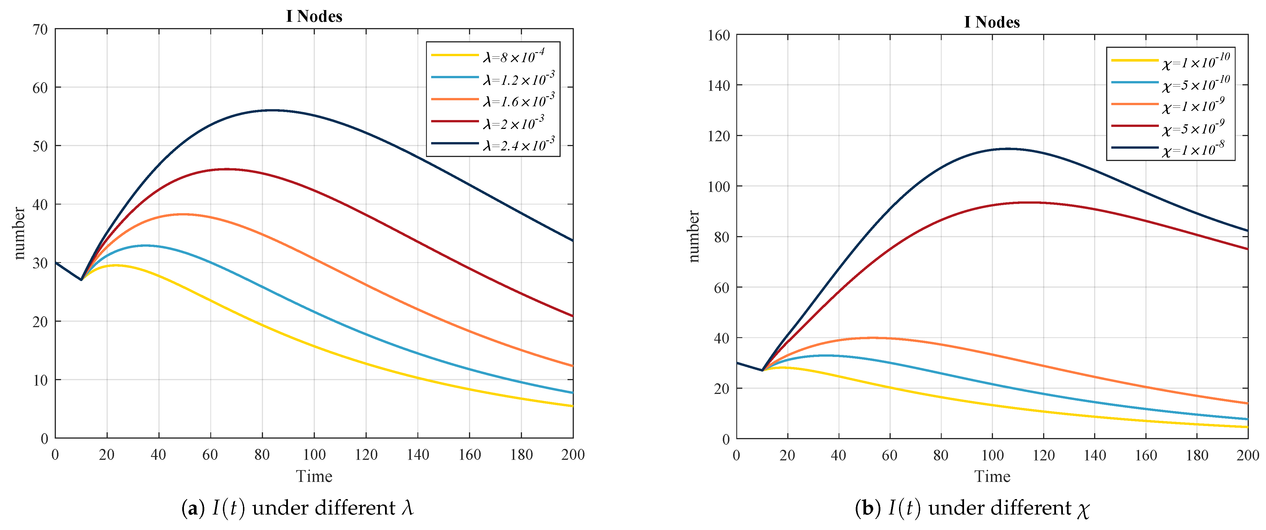
Analysis of Node Density $\gamma$ and Transmit Power Coefficient $\chi$ Impact on Epidemic Propagation Dynamics: The influence of different node density $\lambda$ and transmit power coefficient $\chi$ on the VCISQ mathematical model are analyzed under constant control variables ($u_1$ and $u_2$). Specifically, the changes in infected node I under different values of $\lambda$ and $\chi$ are analyzed. This comparative experiment is added to demonstrate the rationality and effectiveness of the mathematical model.

3.

Comparison of Costs Under Different Control Strategies: By comparing the performance of the hybrid control strategy (Theorem 2) with two single-control strategies (patching-only control in Theorem 3 and quarantine-only control in Theorem 4), we demonstrate the superiority of hybrid control in suppressing malware propagation and minimizing control costs.

4.

Stability Analysis: We validate the stability and robustness of the model (Figure 1) under different parameter conditions by adjusting two key parameters (the density of total nodes $\lambda$ and transmit power coefficient $\chi$).

5.

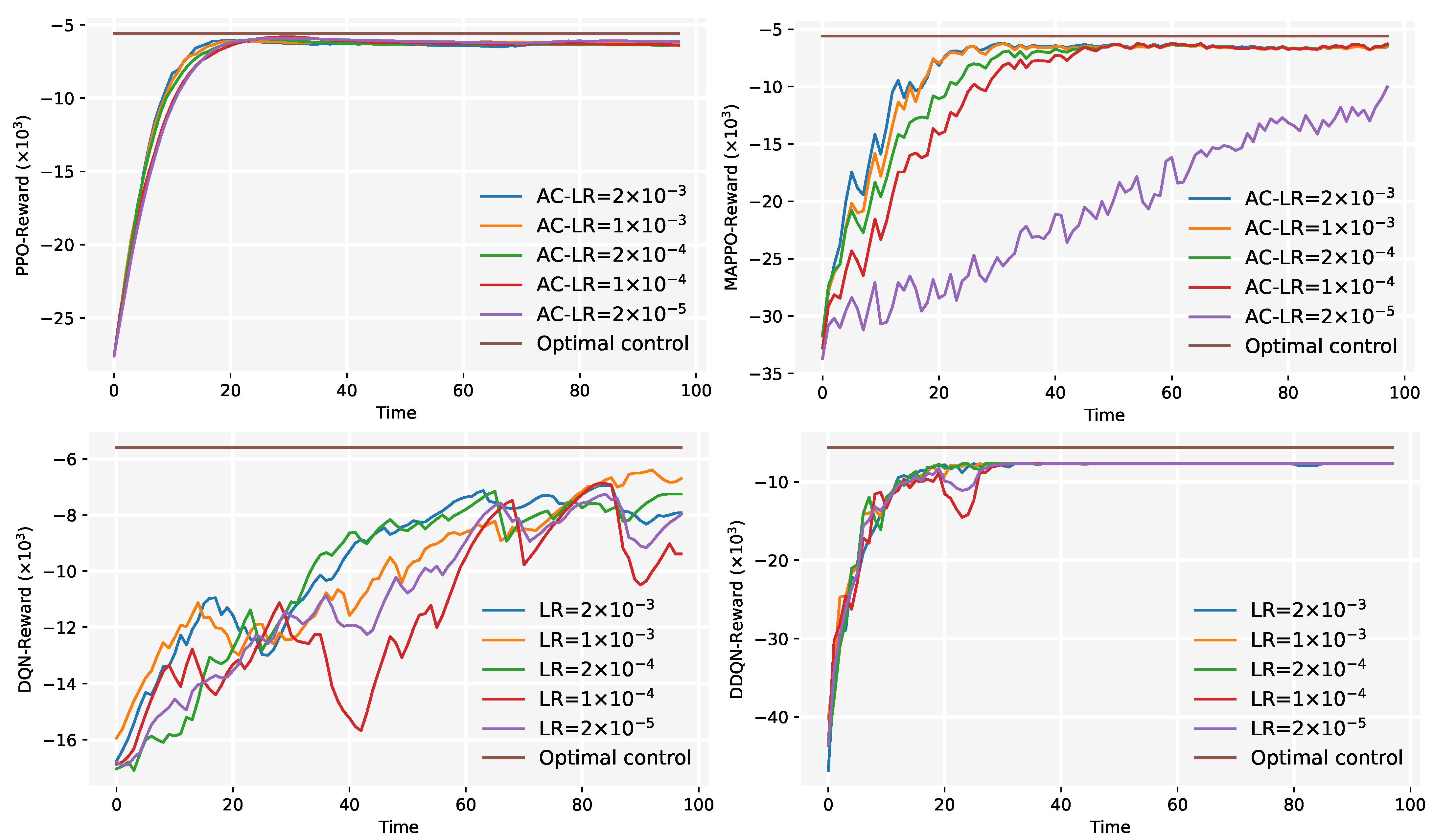
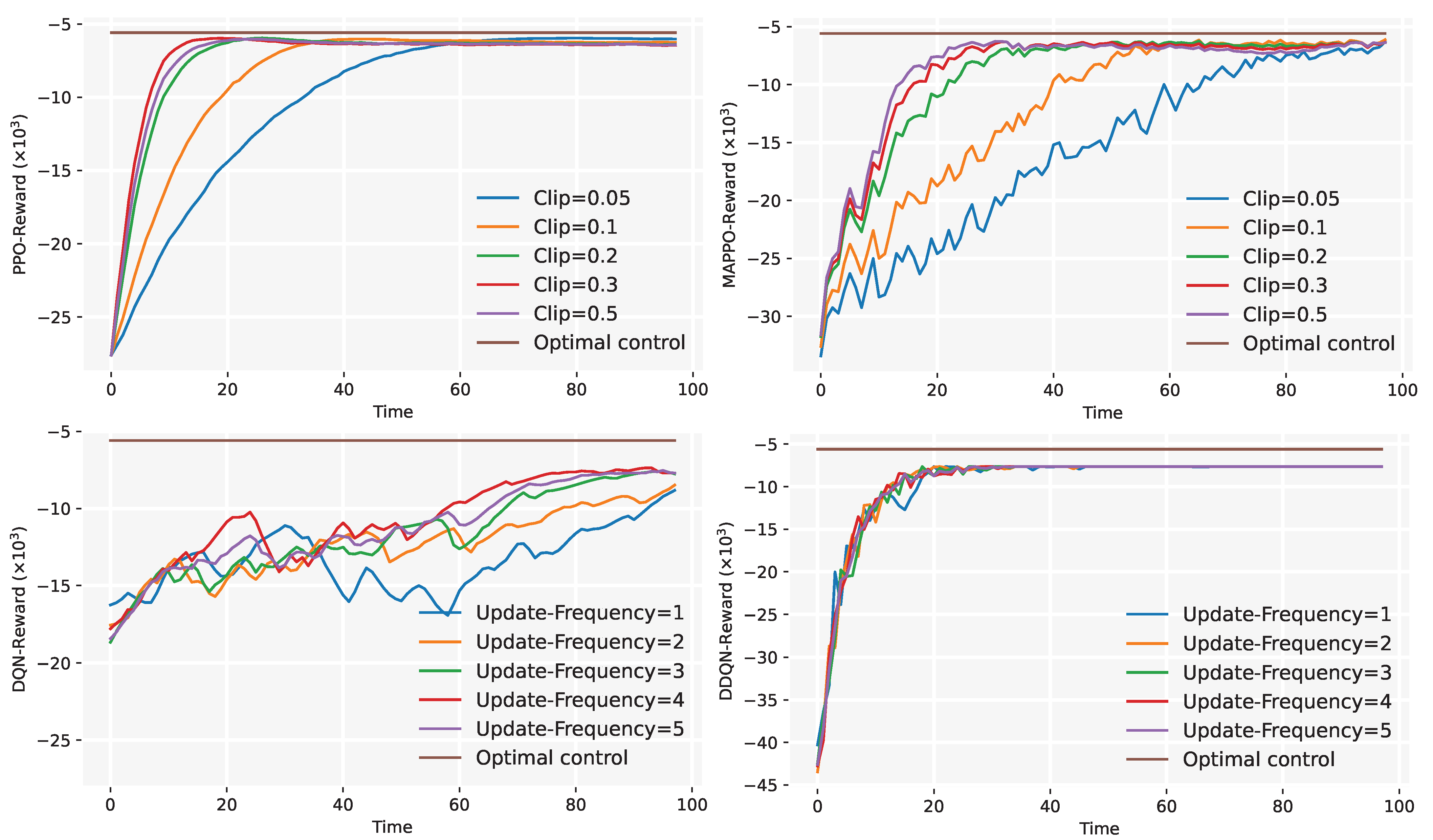
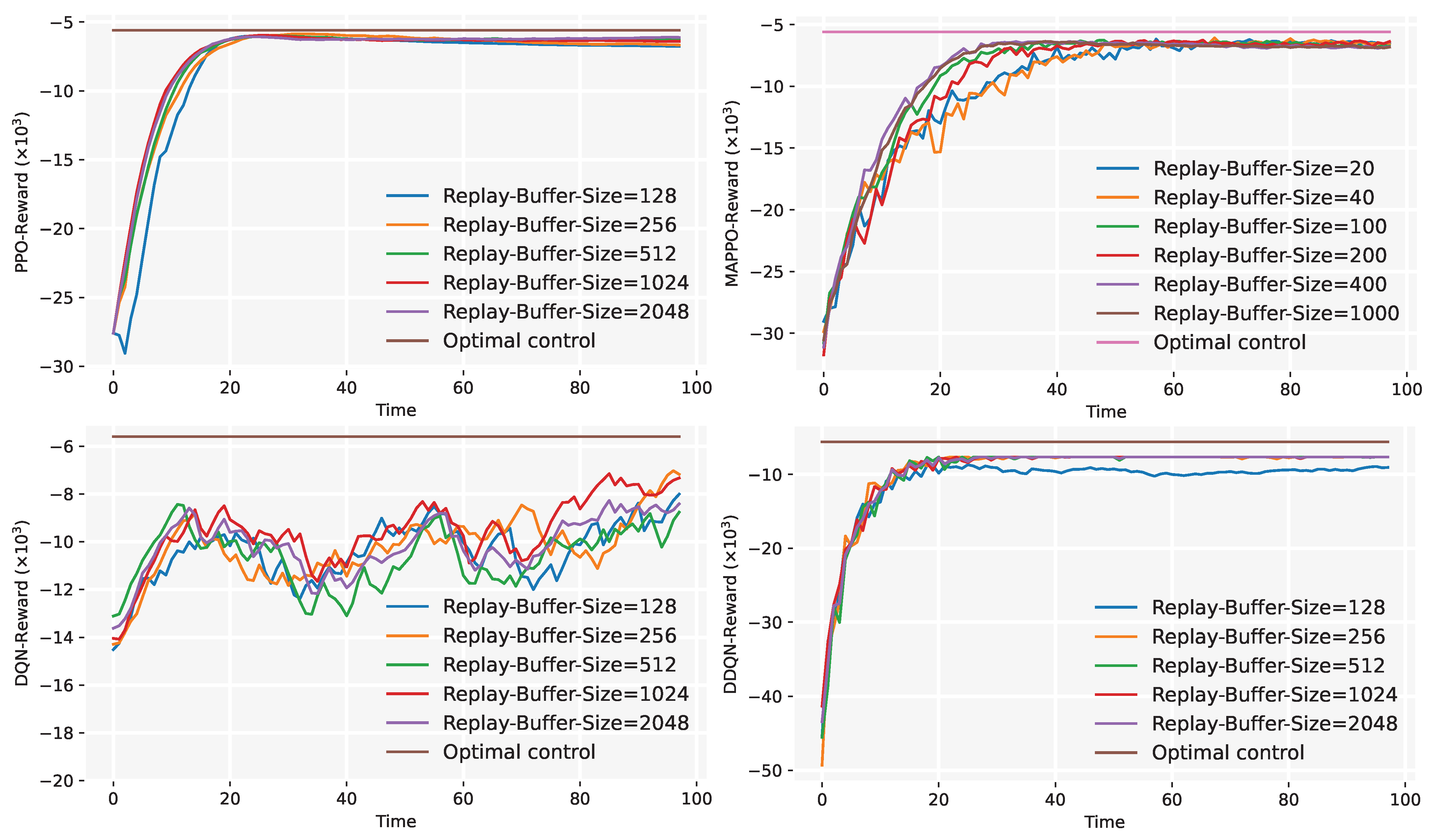
Convergence Experiment: We analyze the convergence performance of PPO (Section 4.1) and MAPPO (Section 4.2) by varying algorithm hyperparameters, optimizing algorithm configurations to improve training efficiency.

6.

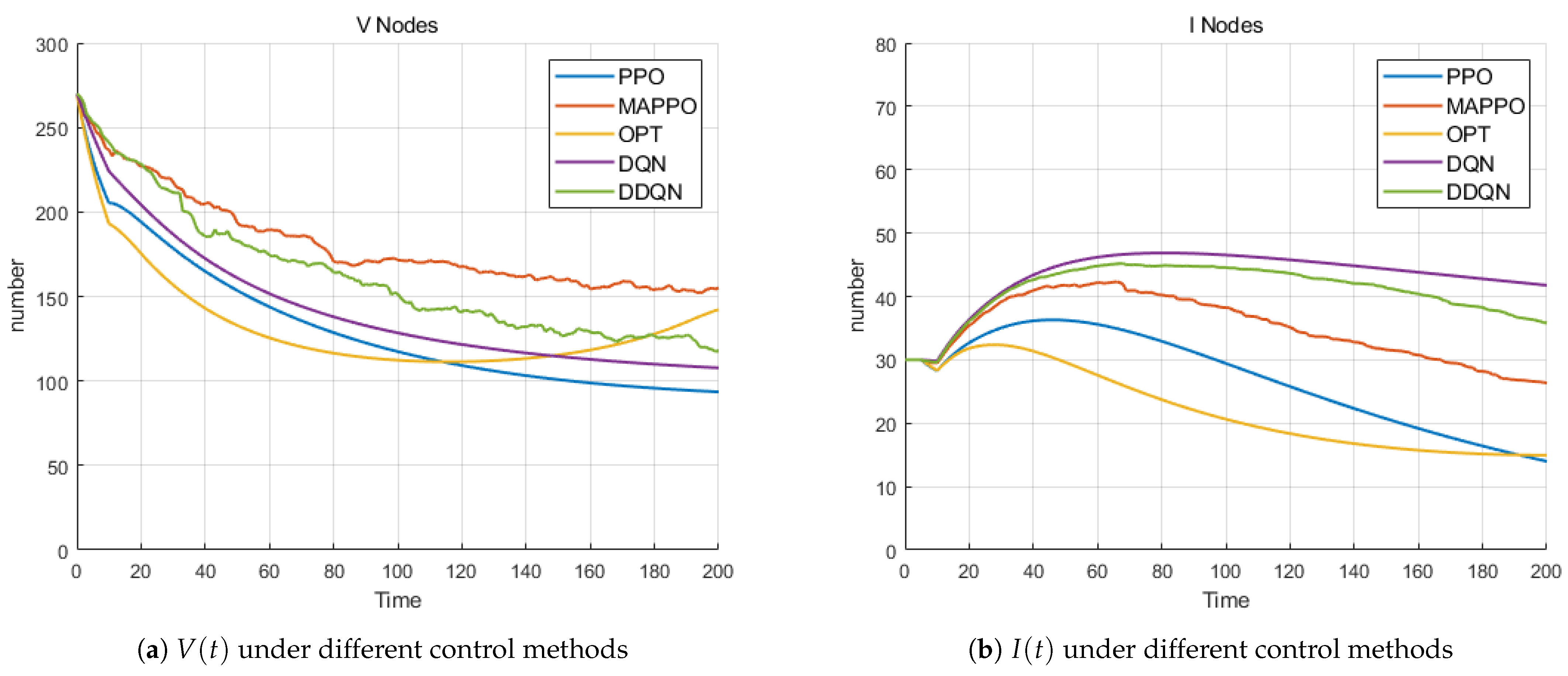
Comparison Of Various Algorithms: We verify the significant advantages of PPO (Section 4.1) and MAPPO (Section 4.2) in control accuracy, learning capability, and adaptability by comparing traditional RL algorithms with optimal control in terms of cost.

In the numerical simulations, the initial values of the relevant nodes in the model were set as $V\left(t\right)=N-30$ and $I\left(t\right)=30$, while the initial values of other nodes were set to 0. The values of other parameters are shown in Table 3.

5.1. Impact of Removing Time Delay

In this experiment, we investigate the effect of eliminating time delays on the performance of the optimal control strategy (Theorem 2) and the overall dynamics of the proposed model. Time delay is a prevalent phenomenon in many real-world systems, particularly in communication and control processes, where decisions are often based on outdated or delayed information. The presence of time delay can lead to instability and inefficiency in the control system.Therefore, understanding its impact is critical for optimizing system performance.

To evaluate the effect of time delay, we conduct simulations both with and without incorporating time delays into the control model. Specifically, we remove the time delay term from the system equations and observe how this alteration influences the effectiveness of the optimal control strategy. We compare the system’s stability under different conditions, aiming to demonstrate whether removing the time delay improves control performance or brings other benefits. The results will provide deeper insights into the role of time delay factors in optimizing information dissemination models, especially in scenarios where rapid responses are critical.

Due to the model’s complexity, a key parameter in the model, the I-nodes representing the infected nodes by the malicious program, is used as a reference for the experiments. In Figure 3a, we compare the impact of introducing time delay on the I-nodes control curve, where all time delay values in the “no-delay” curve are set to zero. The experimental results indicate that, under the combined control strategy, the curve with time delay shows an I-nodes count similar to the curve without time delay, though the balance value of the I-nodes is slightly lower when time delay is introduced.

In Figure 3b, we demonstrate the effect of increasing the delay in the installation of the malicious program on the I-nodes. As the delay increases, the equilibrium number of I-nodes steadily increases. This suggests that adding delay to the installation process of the malicious program leads to worse performance of the optimal control strategy. However, the increased delay in installation also causes the number of I-nodes in the initial propagation phase to decrease, maintaining a lower I-nodes count throughout the process.

In Figure 3c, the impact of increasing the delay in patch installation on the I-nodes is explored. The results show that as the installation delay increases, the equilibrium number of I-nodes decreases. The delay in patch installation reduces the effectiveness of countermeasures, causing more I-nodes to increase in number during the early stages of propagation, leading to faster spreading.

Figure 3d investigates the effect of increasing the patch failure delay. The experimental results indicate that as the failure delay increases, the equilibrium number of I-nodes decreases, but the magnitude of the decrease is relatively small. This suggests that although the delay in patch failure does influence the number of affected nodes, its impact is less significant compared to the installation delay.

Overall, these experiments provide valuable insights into the effects of time delay in different aspects of the control system. While the removal of time delay results in a slight improvement in system stability, the introduction of time delay in malicious program installation and patching processes has a more significant impact on the equilibrium number of I-nodes. The results emphasize the importance of minimizing time delays in defense mechanisms and response times to maintain system stability and control efficiency.

5.2. Analysis of Node Density $\lambda$ and Transmit Power Coefficient $\chi$ Impact on Epidemic Propagation Dynamics

To validate the model rationality and parameter sensitivity, this section investigates the influence of total node density $\lambda$ on infectious disease propagation dynamics through numerical simulations. With control parameters held constant ($u_1$ = 0.1, $u_2$ = 0.1) and other system parameters configured according to Table 3, Figure 4a illustrates the temporal evolution curves of I-nodes under varying node densities ($\lambda$ = 8 $\times {10}^{-4}$, 1.2 $\times {10}^{-3}$, 1.6 $\times {10}^{-3}$, 2 $\times {10}^{-3}$, 2.4 $\times {10}^{-3}$).

Numerical simulations demonstrate that increased node density $\lambda$ induces remarkable transmission acceleration phenomena. As $\lambda$ escalates from 8 $\times {10}^{-4}$ to 2.4 $\times {10}^{-3}$, the time required for the network to reach maximum infection intensity decreases by approximately 62%, accompanied by substantial growth in infected node counts across all time phases. These findings confirm that enhanced nodal density simultaneously accelerates epidemic progression and amplifies final infection magnitude.

As a critical parameter in radar channel communications, the transmit power coefficient $\chi$ exerts substantial influence on coupling parameters in Equations (1) and (2) by modulating channel gain and signal interference levels.

Under fixed control strategies ($u_1$ = 0.1, $u_2$ = 0.1) and parameter settings from Table 3, Figure 4b presents the propagation dynamics evolution for different transmit power coefficients ($\chi$ = 1 $\times {10}^{-10}$, 5 $\times {10}^{-10}$, 1 $\times {10}^{-9}$, 5 $\times {10}^{-9}$, 1 $\times {10}^{-8}$). The results reveal a positive correlation between $\chi$ values and infection rates. Notably, when $\chi$ exceeds 1 $\times {10}^{-9}$, both infection velocity and stabilized infected node quantities exhibit exponential growth. This nonlinear response characteristic suggests that judicious regulation of transmission power holds significant engineering implications for epidemic containment strategies.

5.3. Comparison of Costs Under Different Control Strategies

To validate the effectiveness of the hybrid control strategy, this section compares the control effects of the hybrid control strategy (Theorem 2), the single quarantine-control strategy (Theorem 3), and the single patching-control strategy (Theorem 4). The total control cost of the model is used as the metric to evaluate the optimal control problem. The optimal solutions for ${u_1}^{opt}$, ${u_2}^{opt}$, single ${u_1}^{opt}$, and single ${u_2}^{opt}$ are provided in Section 3.4, respectively.

As shown in

Table 4. The cost of optimal control and various RL controls under different channel parameters.

Control	Total Value	Optimal	PPO	MAPPO	DQN	DDQN
	Case
Theorem 2: The Hybrid Optimal Control (Patching-control $u_1$ and Quarantine- control $u_2$)	$\lambda$ = 8 $\times {10}^{-4}$, $\chi$ = 5 $\times {10}^{-10}$	5461.56	5780.12	6075.45	7554.78	7372.23
	$\lambda$ = 1.2 $\times {10}^{-3}$, $\chi$ = 5 $\times {10}^{-10}$	5595.64	5955.67	6456.52	7197.03	7145.24
	$\lambda$ = 1.6 $\times {10}^{-3}$, $\chi$ = 5 $\times {10}^{-10}$	5768.76	6107.56	6876.89	7398.34	7111.67
	$\lambda$ = 2 $\times {10}^{-3}$, $\chi$ = 5 $\times {10}^{-10}$	5969.37	6356.90	6991.15	8804.48	7575.72
	$\lambda$ = 2.4 $\times {10}^{-3}$, $\chi$ = 5 $\times {10}^{-10}$	6175.36	6601.59	7382.83	8894.17	7537.42
	$\lambda$ = 1.2 $\times {10}^{-3}$, $\chi$ = 1 $\times {10}^{-10}$	5384.65	5671.98	5945.31	6682.54	7687.87
	$\lambda$ = 1.2 $\times {10}^{-3}$, $\chi$ = 5 $\times {10}^{-10}$	5595.64	5955.67	6456.52	7197.03	7145.24
	$\lambda$ = 1.2 $\times {10}^{-3}$, $\chi$ = 1 $\times {10}^{-9}$	5815.20	6250.53	6724.76	7101.99	7603.14
	$\lambda$ = 1.2 $\times {10}^{-3}$, $\chi$ = 5 $\times {10}^{-9}$	6653.47	7288.70	7930.25	8329.58	8026.81
	$\lambda$ = 1.2 $\times {10}^{-3}$, $\chi$ = 1 $\times {10}^{-8}$	6805.33	7762.66	8251.92	8438.19	7949.44
Theorem 3: Single Control (Patching-control $u_1$) $u_2$ = 0.1	$\lambda$ = 8 $\times {10}^{-4}$, $\chi$ = 5 $\times {10}^{-10}$	5488.77	5866.91	5945.22	6384.55	7657.46
	$\lambda$ = 1.2 $\times {10}^{-3}$, $\chi$ = 5 $\times {10}^{-10}$	5626.74	6019.01	6183.70	6514.57	7605.31
	$\lambda$ = 1.6 $\times {10}^{-3}$, $\chi$ = 5 $\times {10}^{-10}$	5811.79	6247.24	6548.57	6840.80	7539.13
	$\lambda$ = 2 $\times {10}^{-3}$, $\chi$ = 5 $\times {10}^{-10}$	6033.49	6433.73	6935.26	7368.60	7464.84
	$\lambda$ = 2.4 $\times {10}^{-3}$, $\chi$ = 5 $\times {10}^{-10}$	6262.18	6721.43	7290.69	7612.93	7384.16
	$\lambda$ = 1.2 $\times {10}^{-3}$, $\chi$ = 1 $\times {10}^{-10}$	5422.41	5802.64	5852.97	6253.30	7434.63
	$\lambda$ = 1.2 $\times {10}^{-3}$, $\chi$ = 5 $\times {10}^{-10}$	5626.74	6019.01	6183.70	6514.57	7605.31
	$\lambda$ = 1.2 $\times {10}^{-3}$, $\chi$ = 1 $\times {10}^{-9}$	5862.66	6254.96	6634.21	6973.52	7521.75
	$\lambda$ = 1.2 $\times {10}^{-3}$, $\chi$ = 5 $\times {10}^{-9}$	6790.98	7246.29	8149.71	8614.75	8642.31
	$\lambda$ = 1.2 $\times {10}^{-3}$, $\chi$ = 1 $\times {10}^{-8}$	6937.94	7477.61	8374.90	8887.46	8981.14
Theorem 4: Single Control (Quarantine-control $u_2$) $u_1$ = 0.1	$\lambda$ = 8 $\times {10}^{-4}$, $\chi$ = 5 $\times {10}^{-10}$	5680.24	5811.79	6006.21	6375.27	5991.35
	$\lambda$ = 1.2 $\times {10}^{-3}$, $\chi$ = 5 $\times {10}^{-10}$	5776.77	5930.91	6154.30	6554.67	6211.14
	$\lambda$ = 1.6 $\times {10}^{-3}$, $\chi$ = 5 $\times {10}^{-10}$	5910.32	6078.84	6348.24	6605.91	6940.35
	$\lambda$ = 2 $\times {10}^{-3}$, $\chi$ = 5 $\times {10}^{-10}$	6083.10	6256.74	6609.28	6885.77	6977.84
	$\lambda$ = 2.4 $\times {10}^{-3}$, $\chi$ = 5 $\times {10}^{-10}$	6278.38	6538.30	6876.93	6957.14	7018.47
	$\lambda$ = 1.2 $\times {10}^{-3}$, $\chi$ = 1 $\times {10}^{-10}$	5635.31	5750.58	5952.34	6452.54	5992.79
	$\lambda$ = 1.2 $\times {10}^{-3}$, $\chi$ = 5 $\times {10}^{-10}$	5776.77	5930.91	6154.30	6554.67	6211.14
	$\lambda$ = 1.2 $\times {10}^{-3}$, $\chi$ = 1 $\times {10}^{-9}$	5949.41	6153.15	6408.25	6314.20	6253.04
	$\lambda$ = 1.2 $\times {10}^{-3}$, $\chi$ = 5 $\times {10}^{-9}$	6825.21	7350.12	7734.18	7874.58	7843.41
	$\lambda$ = 1.2 $\times {10}^{-3}$, $\chi$ = 1 $\times {10}^{-8}$	7064.30	7480.24	8094.19	8534.73	8204.58

, under the same conditions (taking $\lambda$ = 8 $\times {10}^{-4}$ and $\chi$ = 5 $\times {10}^{-10}$ as an example), the total cost of the hybrid optimal control is 5461.56. The cost of the single patching-control is 5488.77, which is 27.21 higher than the hybrid optimal control. The cost of the single quarantine-control is 5680.24, which is 218.68 higher than the hybrid control. Furthermore, when comparing the costs of the three control strategies under other identical cases, we find that regardless of the scenario, the hybrid control strategy always results in lower costs and better control performance than the single control strategies.

5.4. Stability Analysis

In this section, to evaluate the sensitivity of the model and the optimal control strategy to key parameters, we adjusted two important parameters: the density of total nodes $\lambda$ and transmit power coefficient $\chi$. Simultaneously, to validate the performance of the optimal control strategy, we compared the node states of the model and the action values of the optimal control under different parameter settings.

As shown in Figure 5, as the density of total nodes $\lambda$ increases, the number of I-nodes rises significantly and the total control cost in Table 4 also increases. This phenomenon indicates that total node density has a significant impact on the propagation dynamics of the channel model. Further analysis of the optimal control action values reveals that as $\lambda$ increases, the variation in patching-control $u_1$ is more pronounced, while the variation in quarantine-control $u_2$ is relatively smaller. This suggests that the increase in node density primarily affects the optimization of the patching-control strategy, while its impact on quarantine-control is more limited.

As shown in Figure 6, as the transmit power coefficient $\chi$ increases, the number of I-nodes also rises significantly, and the magnitude of this increase is much greater than that observed with changes in node density. This indicates that transmission power has a more pronounced impact on the propagation dynamics of the channel model. Additionally, as $\chi$ increases, both the patching-control $u_1$ and quarantine-control $u_2$ of the optimal control strategy exhibit significant variations. This demonstrates that changes in transmission power simultaneously and significantly affect the optimization of both patching- and quarantine-controls. Due to the more pronounced impact of transmission power variations on the control strategy, the system exhibits higher sensitivity and relatively poorer stability.

5.5. Convergence Experiment

In this section, the training iterations for PPO, MAPPO, DQN, and DDQN were set to 100 times. The convergence was evaluated by observing the training reward curve.

The learning rate is the most critical hyperparameter that affects the performance of RL. As shown in Figure 7, PPO and MAPPO still converge under different learning rates for the policy network (A-LR) and the value network (C-LR). As the learning rate decreases, the convergence speed slows down. Among them, PPO is less affected by the learning rate, while MAPPO’s convergence is more sensitive to the learning rate. The convergence curve of DQN fluctuates significantly, resulting in poorer convergence performance. As the upgraded version, DDQN shows a smoother convergence curve with better convergence performance.

In Figure 8, the clip value in PPO is adjusted to prevent significant changes in the policy and value functions between iterations. The clipping strength is controlled by the hyperparameter “clip”, where a larger clipping strength results in larger updates to the policy and value functions. As shown in Figure 8, PPO and MAPPO still converge under different clipping parameters. In contrast to PPO and MAPPO, the update frequency of DQN and DDQN algorithms is treated as a variable in the convergence experiments. The experimental results still show that DQN has poor convergence, while DDQN exhibits better convergence with minimal sensitivity to the changes.

In Figure 9, the convergence behavior under different experience buffer sizes is analyzed. The results show that the experience buffer size has little effect on the convergence speed and final convergence performance of PPO, MAPPO, DQN, and DDQN. As shown in Figure 10, the convergence behavior is compared under different minimum training batch sizes. The minimum training batch size has a minimal impact on the convergence speed and final convergence performance of PPO, MAPPO, and DDQN, while it significantly affects the convergence performance of DQN.

5.6. Comparison of Various Algorithms

In this session, the convergence curves and optimal values of different algorithms under the same parameter conditions are compared. In addition to PPO and MAPPO, traditional RL algorithms DQN and DDQN in RL algorithms are also used to compare convergence.

As model-free deep RL algorithms, DQN and DDQN are widely used for decision-making in complex environments. These algorithms utilize a deep neural network to approximate the Q-value function, which helps in determining the optimal action for an agent. DQN enhances the ability of agent to explore the environment by leveraging experience replay, where past experiences are stored and used for training, leading to improved performance. DDQN, an extension of DQN, mitigates the overestimation bias of the Q-values in DQN, resulting in more stable learning and improved performance, particularly in environments with large action spaces.

In the proposed model, the key nodes, denoted as V and I, serve as the primary control indicators. As illustrated in Figure 11, the propagation graphs for the V-nodes and I-nodes under different algorithms with the same parameters ($\lambda$ = 1.2 $\times {10}^{-3}$ and $\chi$ = 5 $\times {10}^{-10}$) are presented. In Figure 11b, it is observed that the optimal control results in the fewest I-nodes, followed by PPO, MAPPO, DDQN, and DQN. Correspondingly, the total control costs for each algorithm under the given parameters are shown in Table 4. The total cost for optimal control is 5595.56, while for PPO it is 5955.67, MAPPO yields 6456.52, DDQN results in 7145.24, and DQN reaches 7197.03.

Comparing these results, it is evident that PPO and MAPPO outperform the traditional algorithms, DQN and DDQN, in terms of control performance. This supports the assertion that PPO is highly effective in optimizing control strategies. Furthermore, it is noteworthy that MAPPO shows slightly less favorable performance compared to PPO. This could be attributed to the fact that MAPPO deals with a heterogeneous model rather than a single, homogeneous model, which may introduce additional complexities that slightly impact its performance.

6. Conclusions

The problem of malware propagation in WRSN systems is investigated in this study. An epidemiological model is established to accurately describe the cross-propagation of malware. Based on this model, a hybrid optimal control method is proposed to minimize the control cost by combining patching strategies and quarantine strategies. PPO and MAPPO are introduced to solve the control of model. Additionally, the convergence performance and adaptability of DQN, DDQN, PPO, and MAPPO in the control of the infection model are compared.

Simulation results show that hybrid control is superior to single control. The malware installation delay and patch installation delay in the network have a significant impact on the control effect of the model. The learning rate and clipping parameter of the network have a great influence on the convergence performance of PPO and MAPPO algorithms. In terms of controlling malware propagation, PPO shows cost-effectiveness advantages over MAPPO. Especially when facing changes in key parameters such as the density of total nodes and the transmit power coefficient, PPO exhibits better adaptability performance. Simulation results showed that the learning rate and clipping parameter of the network had a greater impact on the convergence performance of PPO and MAPPO algorithms. PPO exhibited cost-effective advantages over MAPPO in controlling malware propagation. Especially when facing changes in key parameters such as malware propagation rate, patch software failure rate, and successful installation rate, PPO demonstrated better adaptability performance.

Currently, we plan to explore the higher-dimension application of heterogeneous sensor networks in malware propagation. This exploration not only enriches the research in the field of WRSNs but also has far-reaching implications for other domains. For example, in the smart healthcare industry, where sensor networks are widely used to monitor patients’ health conditions, understanding malware propagation in heterogeneous sensor networks can help safeguard the security of patient data. Malware attacks could potentially disrupt the accurate transmission of medical data, endangering patients’ lives. In addition, network attacks in real-world scenarios often possesses adversarial capabilities. To better align with such situations, adversarial attack conditions will be analyzed in our future study. Game theory-based RL will also be utilized to investigate how RL methods can achieve more robust strategies in adversarial attacks. This approach aims to produce more stable control outcomes and more effectively suppress the spread of network attacks.

References

- Akan, O.B.; Arik, M. Internet of Radars: Sensing versus Sending with Joint Radar-Communications. IEEE Commun. Mag. 2020, 58, 13–19. [Google Scholar] [CrossRef]
- Luo, F.; Bodanese, E.; Khan, S.; Wu, K. Spectro-Temporal Modeling for Human Activity Recognition Using a Radar Sensor Network. IEEE Trans. Geosci. Remote Sens. 2023, 61, 5103913. [Google Scholar] [CrossRef]
- Bartoletti, S.; Conti, A.; Giorgetti, A.; Win, M.Z. Sensor radar networks for indoor tracking. IEEE Wirel. Commun. Lett. 2014, 3, 157–160. [Google Scholar]
- Gulmezoglu, B.; Guldogan, M.B.; Gezici, S. Multiperson tracking with a network of ultrawideband radar sensors based on Gaussian mixture PHD filters. IEEE Sens. J. 2014, 15, 2227–2237. [Google Scholar] [CrossRef]
- Peng, H.; Wang, Y.; Chen, Z.; Lv, Z. Dynamic sensor speed measurement algorithm and influencing factors of traffic safety with wireless sensor network nodes and RFID. IEEE Sens. J. 2020, 21, 15679–15686. [Google Scholar] [CrossRef]
- Primeau, N.; Falcon, R.; Abielmona, R.; Petriu, E.M. A review of computational intelligence techniques in wireless sensor and actuator networks. IEEE Commun. Surv. Tutor. 2018, 20, 2822–2854. [Google Scholar] [CrossRef]
- Haghighi, M.S.; Wen, S.; Xiang, Y.; Quinn, B.; Zhou, W. On the race of worms and patches: Modeling the spread of information in wireless sensor networks. IEEE Trans. Inf. Forensics Secur. 2016, 11, 2854–2865. [Google Scholar] [CrossRef]
- Liu, G.; Peng, Z.; Liang, Z.; Zhong, X.; Xia, X. Analysis and Control of Malware Mutation Model in Wireless Rechargeable Sensor Network with Charging Delay. Mathematics 2022, 10, 2376. [Google Scholar] [CrossRef]
- Liu, G.; Chen, J.; Liang, Z.; Peng, Z.; Li, J. Dynamical Analysis and Optimal Control for a SEIR Model Based on Virus Mutation in WSNs. Mathematics 2021, 9, 929. [Google Scholar] [CrossRef]
- Nwokoye, C.H.; Madhusudanan, V. Epidemic models of malicious-code propagation and control in wireless sensor networks: An indepth review. Wirel. Pers. Commun. 2022, 125, 1827–1856. [Google Scholar] [CrossRef]
- Peng, S.C. A survey on malware containment models in smartphones. Appl. Mech. Mater. 2013, 263, 3005–3011. [Google Scholar] [CrossRef]
- Guillén, J.H.; del Rey, A.M. A mathematical model for malware spread on WSNs with population dynamics. Phys. A Stat. Mech. Its Appl. 2020, 545, 123609. [Google Scholar] [CrossRef]
- Shen, S.; Li, H.; Han, R.; Vasilakos, A.V.; Wang, Y.; Cao, Q. Differential game-based strategies for preventing malware propagation in wireless sensor networks. IEEE Trans. Inf. Forensics Secur. 2014, 9, 1962–1973. [Google Scholar] [CrossRef]
- Bai, L.; Liu, J.; Han, R.; Zhang, W. Wireless radar sensor networks: Epidemiological modeling and optimization. IEEE J. Sel. Areas Commun. 2022, 40, 1993–2005. [Google Scholar] [CrossRef]
- Liu, X.; Yang, L. Stability analysis of an SEIQV epidemic model with saturated incidence rate. Nonlinear Anal. Real World Appl. 2012, 13, 2671–2679. [Google Scholar] [CrossRef]
- Sun, A.; Sun, C.; Du, J.; Wei, D. Optimizing Energy Efficiency in UAV-Assisted Wireless Sensor Networks with Reinforcement Learning PPO2 Algorithm. IEEE Sens. J. 2023, 23, 29705–29721. [Google Scholar] [CrossRef]
- Kuai, Z.; Wang, T.; Wang, S. Fair virtual network function mapping and scheduling using proximal policy optimization. IEEE Trans. Commun. 2022, 70, 7434–7445. [Google Scholar] [CrossRef]
- Xiao, J.; Chen, Z.; Sun, X.; Zhan, W.; Wang, X.; Chen, X. Online Multi-Agent Reinforcement Learning for Multiple Access in Wireless Networks. IEEE Commun. Lett. 2023, 27, 3250–3254. [Google Scholar] [CrossRef]
- Wu, J.; Wei, Z.; Li, W.; Wang, Y.; Li, Y.; Sauer, D.U. Battery Thermal- and Health-Constrained Energy Management for Hybrid Electric Bus Based on Soft Actor-Critic DRL Algorithm. IEEE Trans. Ind. Inform. 2021, 17, 3751–3761. [Google Scholar] [CrossRef]
- Rakelly, K.; Zhou, A.; Finn, C.; Levine, S.; Quillen, D. Efficient off-policy meta-reinforcement learning via probabilistic context variables. In Proceedings of the International Conference on Machine Learning, Long Beach, CA, USA, 9–15 June 2019; pp. 5331–5340. [Google Scholar]
- Xiao, X.; Fu, P.; Dou, C.; Li, Q.; Hu, G.; Xia, S. Design and analysis of SEIQR worm propagation model in mobile internet. Commun. Nonlinear Sci. Numer. Simul. 2017, 43, 341–350. [Google Scholar] [CrossRef]
- Liu, G.; Zhang, J.; Zhong, X.; Hu, X.; Liang, Z. Hybrid optimal control for malware propagation in UAV-WSN system: A stacking ensemble learning control algorithm. IEEE Internet Things J. 2024, 11, 36549–36568. [Google Scholar] [CrossRef]
- Keshri, N.; Mishra, B.K. Two time-delay dynamic model on the transmission of malicious signals in wireless sensor network. Chaos Solitons Fractals 2014, 68, 151–158. [Google Scholar] [CrossRef]
- Zhuang, Q.; Xiao, M.; Ding, J.; Yang, Q.; Cao, J.; Zheng, W.X. Spatiotemporal Evolution Control of Malicious Virus Propagation in Cyber Physical Systems Via PD Feedback Control. IEEE Trans. Control Netw. Syst. 2023, 11, 1562–1575. [Google Scholar] [CrossRef]
- Shen, S.; Xie, L.; Zhang, Y.; Wu, G.; Zhang, H.; Yu, S. Joint Differential Game and Double Deep Q-Networks for Suppressing Malware Spread in Industrial Internet of Things. IEEE Trans. Inf. Forensics Secur. 2023, 18, 5302–5315. [Google Scholar] [CrossRef]
- Zhong, X.; Yang, Y.; Deng, F.; Liu, G. Rumor Propagation Control With Anti-Rumor Mechanism and Intermittent Control Strategies. IEEE Trans. Comput. Soc. Syst. 2024, 11, 2397–2409. [Google Scholar] [CrossRef]
- Zhong, X.; Pang, B.; Deng, F.; Zhao, X. Hybrid stochastic control strategy by two-layer networks for dissipating urban traffic congestion. Sci. China Inf. Sci. 2024, 67, 140204. [Google Scholar] [CrossRef]
- Cui, S.; Dong, C.; Shen, M.; Liu, Y.; Jiang, B.; Lu, Z. CBSeq: A Channel-Level Behavior Sequence for Encrypted Malware Traffic Detection. IEEE Trans. Inf. Forensics Secur. 2023, 18, 5011–5025. [Google Scholar] [CrossRef]
- He, Y.; Kang, X.; Yan, Q.; Li, E. ResNeXt+: Attention Mechanisms Based on ResNeXt for Malware Detection and Classification. IEEE Trans. Inf. Forensics Secur. 2024, 19, 1142–1155. [Google Scholar] [CrossRef]
- Chen, X.; Hao, Z.; Li, L.; Cui, L.; Zhu, Y.; Ding, Z.; Liu, Y. CruParamer: Learning on Parameter-Augmented API Sequences for Malware Detection. IEEE Trans. Inf. Forensics Secur. 2022, 17, 788–803. [Google Scholar] [CrossRef]
- Tian, B.; Jiang, J.; He, Z.; Yuan, X.; Dong, L.; Sun, C. Functionality-Verification Attack Framework Based on Reinforcement Learning Against Static Malware Detectors. IEEE Trans. Inf. Forensics Secur. 2024, 19, 8500–8514. [Google Scholar] [CrossRef]
- Farooq, M.J.; Zhu, Q. Modeling, analysis, and mitigation of dynamic botnet formation in wireless IoT networks. IEEE Trans. Inf. Forensics Secur. 2019, 14, 2412–2426. [Google Scholar] [CrossRef]
- Gao, Q.; Zhuang, J. Stability analysis and control strategies for worm attack in mobile networks via a VEIQS propagation model. Appl. Math. Comput. 2020, 368, 124584. [Google Scholar] [CrossRef]
- Ding, L.; Hu, P.; Guan, Z.H.; Li, T. An efficient hybrid control strategy for restraining rumor spreading. IEEE Trans. Syst. Man, Cybern. Syst. 2020, 51, 6779–6791. [Google Scholar] [CrossRef]
- Liu, G.; Li, H.; Xiong, L.; Tan, Z.; Liang, Z.; Zhong, X. Fractional-Order Optimal Control and FIOV-MASAC Reinforcement Learning for Combating Malware Spread in Internet of Vehicles. IEEE Trans. Autom. Sci. Eng. 2025, 22, 10313–10332. [Google Scholar] [CrossRef]
- Gu, Y.; Guo, K.; Zhao, C.; Yu, X.; Guo, L. Fast Reactive Mechanism for Desired Trajectory Attacks on Unmanned Aerial Vehicles. IEEE Trans. Ind. Inform. 2023, 19, 8976–8984. [Google Scholar] [CrossRef]
- Han, S.; Zhao, H.; Li, X.; Yu, J.; Liu, Z.; Yan, L.; Zhang, T. Joint Multiple Resources Allocation for Underwater Acoustic Cooperative Communication in Time-Varying IoUT Systems: A Double Closed-Loop Adversarial Bandit Approach. IEEE Internet Things J. 2024, 11, 2573–2587. [Google Scholar] [CrossRef]
- Heidari, A.; Jamali, M.A.J. Internet of Things intrusion detection systems: A comprehensive review and future directions. Clust. Comput. 2023, 26, 3753–3780. [Google Scholar] [CrossRef]
- Chai, Y.; Wang, Y. Optimal Control of Information Diffusion in Temporal Networks. IEEE Trans. Netw. Serv. Manag. 2023, 20, 104–119. [Google Scholar] [CrossRef]
- Tayseer Jafar, M.; Yang, L.X.; Li, G.; Zhu, Q.; Gan, C. Minimizing Malware Propagation in Internet of Things Networks: An Optimal Control Using Feedback Loop Approach. IEEE Trans. Inf. Forensics Secur. 2024, 19, 9682–9697. [Google Scholar] [CrossRef]
- Liu, G.; Tan, Z.; Liang, Z.; Chen, H.; Zhong, X. Fractional Optimal Control for Malware Propagation in Internet of Underwater Things. IEEE Internet Things J. 2024, 11, 11632–11651. [Google Scholar] [CrossRef]
- Shen, S.; Cai, C.; Shen, Y.; Wu, X.; Ke, W.; Yu, S. Joint Mean-Field Game and Multiagent Asynchronous Advantage Actor-Critic for Edge Intelligence-Based IoT Malware Propagation Defense. IEEE Trans. Dependable Secur. Comput. 2025, preprints. [Google Scholar] [CrossRef]
- Lee, J.; Cheng, Y.; Niyato, D.; Guan, Y.L.; González, D. Intelligent resource allocation in joint radar-communication with graph neural networks. IEEE Trans. Veh. Technol. 2022, 71, 11120–11135. [Google Scholar] [CrossRef]
- Thornton, C.E.; Kozy, M.A.; Buehrer, R.M.; Martone, A.F.; Sherbondy, K.D. Deep reinforcement learning control for radar detection and tracking in congested spectral environments. IEEE Trans. Cogn. Commun. Netw. 2020, 6, 1335–1349. [Google Scholar] [CrossRef]
- Guo, J.; Jafarkhani, H. Sensor deployment with limited communication range in homogeneous and heterogeneous wireless sensor networks. IEEE Trans. Wirel. Commun. 2016, 15, 6771–6784. [Google Scholar] [CrossRef]
- Guo, J.; Li, M.; Guo, Z.; She, Z. Reinforcement Learning-Based 3-D Sliding Mode Interception Guidance via Proximal Policy Optimization. IEEE J. Miniaturization Air Space Syst. 2023, 4, 423–430. [Google Scholar] [CrossRef]
- Wang, H.; Hao, J.; Wu, W.; Jiang, A.; Mao, K.; Xia, Y. A New AGV Path Planning Method Based On PPO Algorithm. In Proceedings of the 42nd Chinese Control Conference (CCC), Tianjin, China, 24–26 July 2023; pp. 3760–3765. [Google Scholar] [CrossRef]
- Kang, H.; Chang, X.; Mišić, J.; Mišić, V.B.; Fan, J.; Liu, Y. Cooperative UAV Resource Allocation and Task Offloading in Hierarchical Aerial Computing Systems: A MAPPO-Based Approach. IEEE Internet Things J. 2023, 10, 10497–10509. [Google Scholar] [CrossRef]
- Yu, C.; Velu, A.; Vinitsky, E.; Gao, J.; Wang, Y.; Bayen, A.; Wu, Y. The surprising effectiveness of ppo in cooperative multi-agent games. Adv. Neural Inf. Process. Syst. 2022, 35, 24611–24624. [Google Scholar]
- Cui, J.; Liu, Y.; Nallanathan, A. Multi-agent reinforcement learning-based resource allocation for UAV networks. IEEE Trans. Wirel. Commun. 2019, 19, 729–743. [Google Scholar] [CrossRef]
- Jafar, M.T.; Yang, L.X.; Li, G. An innovative practical roadmap for optimal control strategies in malware propagation through the integration of RL with MPC. Comput. Secur. 2025, 148, 104186. [Google Scholar] [CrossRef]
- Ren, Y.; Sun, Y.; Peng, M. Deep Reinforcement Learning Based Computation Offloading in Fog Enabled Industrial Internet of Things. IEEE Trans. Ind. Inform. 2021, 17, 4978–4987. [Google Scholar] [CrossRef]
- Wu, P.; Tian, L.; Zhang, Q.; Mao, B.; Chen, W. MARRGM: Learning Framework for Multi-Agent Reinforcement Learning via Reinforcement Recommendation and Group Modification. IEEE Robot. Autom. Lett. 2024, 9, 5385–5392. [Google Scholar] [CrossRef]
- Chen, H.; Zhu, C.; Tang, R.; Zhang, W.; He, X.; Yu, Y. Large-Scale Interactive Recommendation with Tree-Structured Reinforcement Learning. IEEE Trans. Knowl. Data Eng. 2023, 35, 4018–4032. [Google Scholar] [CrossRef]
- Yang, M.; Wang, Y.; Yu, Y.; Zhou, M.; U, L.H. MixLight: Mixed-Agent Cooperative Reinforcement Learning for Traffic Light Control. IEEE Trans. Ind. Inform. 2024, 20, 2653–2661. [Google Scholar] [CrossRef]
- Kassab, R.; Destounis, A.; Tsilimantos, D.; Debbah, M. Multi-Agent Deep Stochastic Policy Gradient for Event Based Dynamic Spectrum Access. In Proceedings of the 2020 IEEE 31st Annual International Symposium on Personal, Indoor and Mobile Radio Communications, London, UK, 31 August–3 September 2020; pp. 1–6. [Google Scholar] [CrossRef]
- Xu, Y.; Yu, J.; Headley, W.; Buehrer, R. Deep Reinforcement Learning for Dynamic Spectrum Access in Wireless Networks. In Proceedings of the MILCOM 2018–2018 IEEE Military Communications Conference (MILCOM), Los Angeles, CA, USA, 29–31 October 2018; pp. 207–212. [Google Scholar] [CrossRef]
- Han, M.; Sun, X.; Zhan, W.; Gao, Y.; Jiang, Y. Multi-Agent Reinforcement Learning Based Uplink OFDMA for IEEE 802.11ax Networks. IEEE Trans. Wirel. Commun. 2024, 23, 8868–8882. [Google Scholar] [CrossRef]